Abstract
This study quantifies energy consumption and tank-to-wheel (TTW) emissions of urban buses under varying traffic conditions and passenger loads in Osnabrück, Germany, to support emission-aware route assessment in sustainable mobility applications. Exemplary bus trajectories were modeled on a representative 6.17 km route of line M5 (18 m articulated bus; diesel and battery-electric) within a 22.31 km2 traffic net using the Simulation of Urban MObility (SUMO) software, and were calibrated with traffic sensor data. To assess the influence of trajectories in different traffic situations, three different 90 min scenarios were compared (morning peak, noon, night). Trajectory-based energy consumption and greenhouse gas emissions were compared by using the SUMO-implemented emission models HBEFA and PHEMlight, as well as data from the literature. Both diesel and electric buses showed variations in energy consumption depending on the traffic conditions, with generally lower energy consumption for electric propulsion. Temporal differences in the TTW emissions of the diesel bus were modest, with slightly higher morning values, while spatial analysis showed PM peaks in pedestrian zones, NOx peaks during acceleration phases, and CO2 increases after stops and in low-speed areas. The results provide spatially resolved TTW factors for integration into routing applications, excluding upstream and non-exhaust processes in line with the defined system boundary.
1. Introduction
Urban environments are characterized by high population density and traffic-related exposure, but also offer significant potential for emission reduction through sustainable mobility options and adaptive traffic management strategies [1]. For urban environments in particular, mobility plays a vital role in everyday life, where access to work, education, and social participation rely significantly on transport infrastructure and accessibility. At the same time, mobility is associated with substantial energy use and environmental impacts. In Germany, the transport sector alone accounted for 23.3% of total greenhouse gas (GHG) emissions in 2021 [2], with motorized private transport dominating at 75.5% [3]. In addition to GHG emissions, transport activities also generate nitrogen oxides (NOx) and particulate matter (PM). PM also arises from non-exhaust sources such as tire abrasion and braking processes [4]. These emissions not only affect the environment but also pose serious risks to human health [5].
The reduction of carbon emissions in the transport sector relies on regulations on the one hand and incentive systems on the other hand [6]. According to the EU’s “Green Deal” policy framework, the climate targets for the transport sector are a 90% reduction in greenhouse gas-related emissions by 2050 [7]. While electric propulsion based on renewable electricity leads to significant emission reductions in passenger cars and public transport, there is significant potential for savings in modal-split changes to lower-emission mobility options. Against this background, digital mobility services increasingly aim to incorporate environmental criteria into route selection to account for these dynamic, traffic-induced emission characteristics in everyday travel decisions [8,9]. To date, however, this has only been applied to private vehicle travel, while real-time, emission-aware routing for public transport remains largely unexplored. Moreover, routing options labeled as “eco-friendly” are typically defined in a qualitative and non-transparent manner, as they are not tied to explicitly defined emission system boundaries. To put emission-aware routing into practice, an explicit emission system boundary must therefore be defined. One commonly applied boundary in transport emission assessment is in-use, or tank-to-wheel (TTW) emissions, which capture direct exhaust emissions during vehicle operation while excluding upstream processes such as fuel production and distribution (norm ISO 14083 [2023] [10]). This choice does not imply comprehensiveness but provides a practicable and operationally well-defined basis for routing-oriented applications.
Based on this definition, routing-oriented emission assessment requires methods that resolve vehicle operation with sufficient temporal and spatial detail while remaining computationally tractable for real-time or near-real-time use.
Vehicle emissions are mainly produced by fuel combustion in internal combustion engines, leading to gas release. Urban traffic is characterized by low average speeds, frequent stops, and repeated acceleration events, resulting in increased energy consumption and emissions by keeping vehicles outside their optimal operating ranges [11,12].
Emission estimation approaches for public urban bus transport range from on-road testing using Portable Emission Measurement Systems (PEMSs) or chassis dynamometer measurements [11,13,14,15,16,17] to model-based approaches that combine experimental data, such as vehicle trajectories and diagnostic information [18,19,20], real-world traffic data [21], and passenger load factors [12,22] within traffic simulations, environments, or driving-mode modeling frameworks [18,19,20,21,22,23,24,25,26].
Within this methodological landscape, different levels of modeling abstraction have been applied in the literature. Timetable-based approaches enable scalable, city-wide exposure assessments, but neglect dynamically resolved traffic conditions and vehicle operation [26]. Trajectory-based studies show that time-of-day traffic conditions, passenger occupancy, driving behavior, and powertrain choice can substantially influence route-level emissions and energy demand [23,27]. However, these factors are typically examined individually and on a limited spatial scale, while their relative importance for real-time, routing-oriented applications has not yet been systematically assessed.
Rather than re-investigating individual operational factors in isolation, this study addresses a practical implementation question for emission-aware routing in public transport: What level of emission modeling detail is required to provide meaningful routing-relevant emission feedback under realistic urban operating conditions?
The analysis is conducted as an application-oriented case study embedded in the public research project URBANIST [28]. Part of the URBANIST project is the information on time- and space-discretized emissions of different routing and mobility options within urban transportation. Bus trajectories and resulting emissions of an exemplary bus line are modeled in different traffic situations based on microscopic traffic simulation and vehicle count data. Within this framework, the study examines how variability in traffic conditions, passenger occupancy, spatial emission characteristics, modeling granularity, and propulsion technology affects the interpretability of routing-relevant energy consumption and emission information along a representative urban bus corridor, without aiming to derive universally valid emission factors.
2. Materials and Methods
The methodological approach of this study combines empirical data collection with microscopic traffic simulation in SUMO (Simulation of Urban MObility) (German Aerospace Center DLR, Berlin, Germany) to assess routing-relevant bus emissions and to compare the influence of different traffic conditions. Section 2.1 describes the overall model setup, including the study area and traffic data basis (Section 2.1.1), bus and vehicle parameterization based on test trips and manufacturer data (Section 2.1.2), and the simulation framework and traffic demand generation (Section 2.1.3). Section 2.2 introduces the two emission modeling approaches, the Handbook of Emission Factors for Road Transport HBEFA (INFRAS, Bern, Switzerland) and PHEMlight (ITNA TU Graz, Graz, Austria), along with their comparative evaluation. Together, these components enable a controlled yet realistic assessment of tank-to-wheel emissions under varying urban traffic conditions.
2.1. Model Setup
2.1.1. Study Area
The study focuses on the city of Osnabrück in Lower Saxony, Germany, which has approximately 167,000 inhabitants and is the third-largest city in the state. The simulation model covers an area of 22.31 km2, including the inner-city ring, with a total edge length of 268.06 km. The corridor analyzed includes a section of the main street “Iburger Straße” and the inner-city ring (Johannistorwall, Schlosswall, Natruper-Tor-Wall), where traffic is recorded in both directions using TEU (Traffic Eye Universal) detectors (Yunex GmbH, Munich, Germany). The bus line M5 is considered a representative case in estimating the tank-to-wheel emissions of urban bus transport in Osnabrück, simulating one trip direction. The modeled route starts at Kreishaus/Zoo and continues until the bus stop Roopstraße, where the bus leaves the city area and is not further examined. Spanning 6.17 km, the route includes eighteen bus stops (Figure 1, marked with black triangles), two 30 km/h speed zones (dashed in pink), and two pedestrian zones (dashed in blue), in addition to the standard 50 km/h speed limit within German cities.
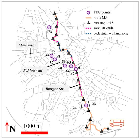
Figure 1.
Study Area. The traffic net, extracted from the SUMO software netedit [29], with the bus route (orange) added, along with its stops (black triangle), the TEU-points (numbers and purple circles), as well as speed limit zones 30 km/h (pink dashed line) and pedestrian zones (blue dashed line).
The City of Osnabrück provided access to historical traffic data from 14 TEU detectors within the study area, covering the period from September 2022 to March 2023. The sensors record vehicle counts and velocities at five-minute intervals. From this dataset, representative daily averages, excluding public holidays, were derived to characterize typical traffic conditions. Figure 2 shows the recorded number of vehicles and their speeds at different times of the day for TEU 61, differentiated by day of the week, with TEU 61 marking the beginning of the inner-city ring. In the figure, weekdays are shown in green and weekends in brown.
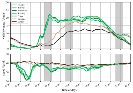
Figure 2.
Vehicle count data (top) and average speed (bottom) against time of day for each day of the week for TEU 61. Weekdays are shown in green and weekends in brown. The nominal speed limit at TEU 61 is 50 km/h. Grey colored background sections mark the investigation intervals.
Weekdays show a steep increase in vehicle counts starting at 06:30, reaching a peak of over 22 vehicles per five-minute interval around 08:00, combined with a decrease in driving speed. At noon, vehicle counts plateau at around 18 vehicles per five-minute interval, with an almost constant overall speed of around 33 km/h. At night, around 21:00, the number of vehicles decreases to eight or fewer vehicles per five-minute interval, with an increased speed of nearly 40 km/h. The traffic behavior during the weekend differs from weekdays but will not be considered further in this study. To capture the different traffic patterns, three 90 min time slots were selected for investigation, with Wednesday as a representative weekday: morning commuter traffic (06:45–08:15), midday traffic (11:00–12:30), and late evening traffic (21:00–22:30). These intervals are highlighted in grey. The count and speed profiles serve as input for lightweight-vehicle traffic demand (excluding trucks) within the simulation setup.
2.1.2. Bus Parameterization
In line with the Osnabrück bus fleet, diesel and electric propulsion were considered as types of drive. The bus operating on route M5 in Osnabrück is an 18-m-long VDL CITEA SLFA-181 electric articulated bus with an empty weight of 18 tons and a passenger capacity of 131 [30,31]. The estimate for the diesel propulsion type was derived from the MAN LION’s CITY 18 [32] combustion engine bus, which has the same properties and a passenger capacity of 150. For simulation consistency, this was set as the default for both propulsion types, along with the MAN bus dimensions of 2.55 m × 3.06 m × 18.06 m. Bus trajectory data was recorded during six test trips, two at each time of day, using a mobile phone device. From that, an average acceleration value of 1.02 m/s2 and a mean deceleration value of 1.14 m/s2 were obtained together with a mean stop duration at each bus stop for each time-of-day scenario (morning: 19.0 s, noon: 14.4 s, night: 12.6 s).
The selected bus route exhibits characteristic features of urban bus operation. The average stop spacing of 343 m lies well within the range reported for international urban bus systems (300–630 m) [33]. In addition, the average operating speeds observed (14.43 ± 0.32 km/h) are comparable to those reported for European cities (14.5 km/h on average) [34]. The route traverses multiple speed limit zones, representing urban traffic heterogeneity.
2.1.3. Simulation Set up
The traffic simulation was set up in SUMO (Simulation of Urban MObility), version 1.21.0 [35]. SUMO is an open-source traffic simulation software distributed under the Eclipse Public License (EPL). The simulation workflow is presented in Figure 3. The road network is based on OpenStreetMap and was obtained using the SUMO-implemented tool, OSM Web Wizard [36]. As the network differs from the actual road connections, crossings, turning options, and traffic light systems, these were configured manually in the test area. The Krauss model [37,38] is the default car-following model used in SUMO and was selected for both vehicle types in this study. For cars, the default parameters were used. For buses, however, the acceleration and deceleration parameter values obtained from the test trips were chosen so that simulated trajectories better match measured trajectories when the engine performance is modeled with PHEMlight to estimate TTW particle emissions.
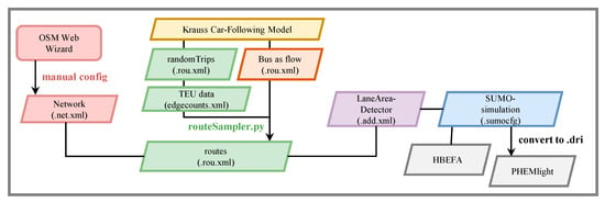
Figure 3.
Simulation workflow. With network configuration (red), car-following model (yellow), traffic demand generation (orange and green), traffic monitoring (violet), actual simulation process (blue), and emission calculation (gray).
The TEU count data was used to define the traffic flow through the network. Specifically, SUMO provides an add-on route sampler that allows users to define the number of vehicles passing through selected edges at a specified time interval. In this case, the time interval is five minutes. The algorithm then generates random trips in accordance with the measured count values at the specified edges, which in this study correspond to the TEU locations. In contrast to the official bus timetable, a bus flow was defined along the route consisting of six buses. The first bus leaves five minutes after the start of the simulation, so that the simulated traffic scenario reflects the real-world demand as best it can. Subsequent buses follow at 12 min intervals.
Additionally, lane area detectors (LADs) were placed in the SUMO model at the TEU positions to monitor the modeled traffic flow along with the velocity of the vehicles passing the detectors. The traffic light system was set dynamically and was not adapted. In total, three 90 min scenarios (morning, noon, night) were simulated. The emission calculation methods HBEFA-4 and PHEMlight V5 are compared in a pre-study for the noon scenario. PHEMlight V5 is a proprietary emission model developed by TU Graz, which was also used to calculate energy consumption.
2.2. Comparison of Emission Calculation Methods
To identify a suitable emission representation for the Osnabrück bus fleet, the possible classes from the Handbook of Emission Factors for Road Transport (HBEFA-4)-based [39] implementation in SUMO, version 1.21.0 [35] and PHEMlight V5 [40] were compared against the CO2 emissions. The comparison focuses on the TTW emissions of diesel Euro VI propulsion. Although both approaches are based on the individual vehicle trajectory within SUMO, they differ fundamentally in their physical representation of vehicle operation. PHEMlight explicitly models engine operation based on vehicle velocity profiles, allowing for a direct representation of operating points along the trajectory. In contrast, the Handbook of Emission Factors for Road Transport (HBEFA) maps vehicle trajectories to predefined traffic situations and assigns aggregated tank-to-wheel emission factors derived from European measurement studies.
Within SUMO, no HBEFA emission class corresponds directly to the articulated 18 t bus operated on the M5 route in Osnabrück. Therefore, two emission classes with the greatest similarity were considered [39]. The articulated bus class Ubus_Artic_gt18t (Euro-VI_A-C), defined for net weights exceeding 18 t, is expected to overestimate emissions for the present application due to its higher reference mass. Conversely, the standard bus class UBus_Std_gt15-18t (Euro-VI_A-C) represents vehicles with net weights between 15 t and 18 t but without articulation, which may lead to an underestimation of the emitted particle emissions. In addition, the HBEFA implementation in SUMO does not allow for weight adaption to represent passenger load variation, limiting the explicit consideration of occupancy effects.
PHEMlight, in contrast, provides the city bus emission class CB_EUVI_D_Heavy for vehicles with weights above 15 t. While articulation is not explicitly specified, PHEMlight allows for passenger mass to be varied in the model definition files, enabling a direct representation of the influence of passenger occupancy that is not possible with the HBEFA-based implementation. A representative passenger load of 17% was assumed, reflecting typical average occupancy levels in urban bus services in Germany (calculated by the federal environment agency of the German government [41], with 17% as the mean value for 2019–2022). Passenger mass was calculated assuming 70 kg per person, following standard practice in transport emission modeling [42,43,44].
To quantify the resulting range of emissions and to identify a suitable emission representation, three influencing factors were investigated:
- deviation between emission models (a);
- the potential influence of a passenger load implementation (b);
- impact of driving parameters (c).
The configurations evaluated and their definitions are summarized in Table 1. The scenario matrix shown was defined specifically for this study, based on the available emission model configurations and the investigated influencing factors. Model identifiers were derived specifically for this study: “H” denotes HBEFA-based and “P” defines PHEMlight-based configurations. Numerical suffixes indicate weight classes, “N” and “G” represent net and gross load conditions, respectively, and “d” denotes the use of default acceleration parameters from SUMO. The latter enables an estimation of the potential influence of the Krauss-model parameter adaptations discussed in the previous section.
In addition to the modeled cases, results were compared with a calculated reference estimate (“calc”). This estimate is based on the net calorific value of diesel at 43.0 TJ/Gg and the corresponding emission factor of 74.1 t CO2/TJ [45]. The fuel consumption was assumed to be 440 g/km, following chassis dynamometer testing values presented in the literature for articulated Euro VI diesel buses [46].

Table 1.
Scenario matrix defined in this study for the comparison of emission models (H—HBEFA, P—PHEMlight, calc—calculated), passenger load representation (N—net, G—gross), and driving parameter variations (a—adapted, d—default).
Table 1.
Scenario matrix defined in this study for the comparison of emission models (H—HBEFA, P—PHEMlight, calc—calculated), passenger load representation (N—net, G—gross), and driving parameter variations (a—adapted, d—default).
| Label | Emission Model | Emission Class | Net Weight /tons | Gross Weight /tons | Acc|Dec /ms−2 |
|---|---|---|---|---|---|
| a—emission models | |||||
| P_15t | PHEMlight | CB_EUVI_D_Heavy [47] | 15 | - | 1.02|1.14 |
| P_18t | 18 | - | 1.02|1.14 | ||
| H_15_18t | HBEFA | UBus_Std_gt15-18t_ Euro-VI_A-C [35] | 15–18 | - | 1.02|1.14 |
| H_gt_18t | >18 | - | 1.02|1.14 | ||
| calc | - | - | - | - | - |
| b—passenger load | |||||
| P_18t_N | PHEMlight | CB_EUVI_D_Heavy [47] | 18 | 1.02|1.14 | |
| P_18t_G | 18 | 19.8 | 1.02|1.14 | ||
| c—driving parameters | |||||
| P_18t_a | PHEMlight | CB_EUVI_D_Heavy [47] | 18 | - | 1.02|1.14 |
| P_18t_d | 18 | - | 2.60|4.50 | ||
3. Results
3.1. Model Validation
3.1.1. Simulation Model
To compare and quantify the different simulation scenarios, private car travel statistics from the SUMO simulation scenarios are summarized in Table 2. Time loss refers to the additional travel time incurred when cars travel below the ideal speed, and waiting time denotes periods in which the car speed is at or below 0.1 m/s. The mean simulated car route length is approximately 2.9 km with a deviation of more than 1 km. Among the three traffic scenarios, the morning peak exhibits the highest average trip duration (421 s), waiting time (74.89 s), and time loss (154.35 s). In addition, the scenarios’ total vehicle count of 10,100 throughout the whole simulation is approximately 2.5 times that of the night scenario. The noon scenario presents very similar traffic volumes (9842 vehicles) and performance indicators (405 s duration, 70.57 s waiting time, 25.62 km/h mean speed, 146.18 s time loss) compared to the morning scenario. In contrast, the night scenario yields the lowest values across all metrics (362 s duration, 40.67 s waiting time, 28.52 km/h mean speed, 101.87 s time loss) with only 4061 vehicles. To prevent gridlocks, SUMO has a safety mechanism of deleting cars from the simulation and inserting them at the next free edge, called teleport [48]. A larger number of teleports may indicate problems with the simulation scenario. Here, the number of vehicle teleports is negligible for all times of day.
Table 2.
Scenario evaluation with metrics towards traffic condition and simulation stability.
The number of vehicles counted at the Lane Area Detectors (LADs) in the simulation is consistent with the input data (error < 1%). The velocities, however, deviate around 17% to 30% on average throughout the day (see Figure 4), with the velocity mostly being overestimated compared to the real-world scenario, indicating a better traffic flow in the simulation model.
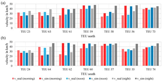
Figure 4.
Velocity comparison for the different times of day. (a) TEU velocities from north to south and (b) opposite direction. Light shades indicate historical velocity data (v_real), and dark shades indicate the average values from the LADs in the simulation (v_sim).
3.1.2. Bus-Flow Behavior
To check whether the simulated bus flow reproduces real-world conditions, travel time and velocity were compared (Figure 5a). In addition, the variation in individual bus trajectories within a scenario was analyzed to verify that multiple buses provide a meaningful statistical basis, without benefiting from the same synchronized green phases at each traffic light system (TLS). Therefore, the number of stops was counted and plotted as a percentage value for each time of day against the corresponding TLS number (Figure 5b).
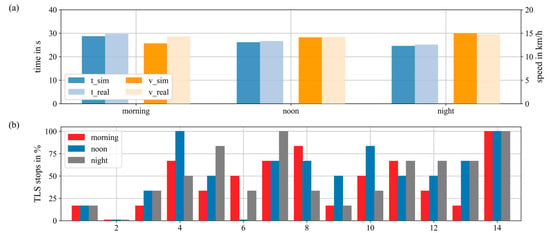
Figure 5.
Bus flow evaluation. (a) Comparison of travel time t (blue) and mean velocity v (orange) from measurements (dark, abbreviated with real) and simulation (light, abbreviated with sim) across scenarios. (b) Stop frequencies at traffic light systems (TLS) expressed as percentages for each TLS and scenario.
According to the real-world measurements, bus travel time was longest in the morning at nearly 30 min, while at night, it was around four minutes shorter, corresponding to a 14% reduction. In contrast, the average bus velocity remained nearly constant throughout the day, with a mean of 14.43 ± 0.32 km/h.
The comparison with the simulation shows only small deviations. Travel time was slightly lower in the simulation, with a deviation of about 2.4%, while the deviation in velocity amounted to 3.1%. These differences can be considered negligible, indicating that the simulation reproduces travel time and velocity behavior with sufficient accuracy.
The TLS stops evaluation shows that, at some TLS, all buses experienced the same TLS condition (e.g., all green in 2, all red in 14), independent of time of day. However, at most TLSs in the simulation, the conditions varied, even within the same scenario. The variation in stop frequencies across traffic light systems indicates that simulated buses experience heterogeneous signal conditions within and across scenarios.
3.1.3. Emission Model: HBEFA vs. PHEMlight
Different influencing factors were considered in finding a suitable representation for the TTW emissions (as discussed in Section 2.2), and then, compared with each other for the noon scenario (see Figure 6). Overall, all the emission values modeled in SUMO exceeded the value calculated by 15 to 58% (see Figure 6a). The modeled values themselves showed the following tendencies: As hypothesized, the largest emissions were found for the articulated HBEFA bus class at 2221 g/km and the lowest for the standard HBEFA bus class (1473 g/km). SUMO reported uncertainty ranges for the HBEFA-based emission values, depicted as error margins. The resulting emissions from PHEMlight for both weight categories lay between the HBEFA values and fell within the standard error margins listed by SUMO. Since the 18-tonne PHEMlight model fulfills the desired criteria for this study (18 tons and adaptable passenger load) and is consistent with the HBEFA values produced, it is used as a practicable reference model to investigate the impact of additional passenger loads (Figure 6b) and the influence of the driving parameters (Figure 6c). Adding a 17% passenger load results in a 5.2% increase. Using the default SUMO driving parameters, the value increases by 6.3%.
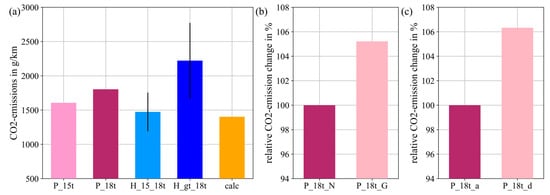
Figure 6.
Influence of emission types and parameter adjustment on direct CO2 emissions for a diesel Euro VI bus at midday. (a) Comparison of the emission methods HBEFA (“H_xxx”, with error margins as vertical lines in black) and PHEMlight (“P_xxx”) with a calculated estimate in g/km; (b) influence of additional passenger load in % (N—net; G—gross); (c) deviation by driving parameter adjustment in % (a—adapted, d—default).
Therefore, adapting the driving parameters can influence the emission results as well as the overall weight, although this is only a minor change compared to the emission model. Nevertheless, for the sake of completeness, it is taken into account. So, the PHEMlight configuration P_18t (parameters see Table 1) is selected for the following analysis with a passenger load of 17% corresponding to the German occupancy average.
3.2. Granularity Considerations
3.2.1. Comparison of Propulsion Type Based on CO2 Emissions in Accordance with Time of Day
In this study, energy consumption served as the comparison parameter between both types of propulsion and also enabled comparison with other studies. In the case of electric propulsion, the consumption was directly derived from the engine power; the corresponding literature value was taken from a research report by the German Government on articulated buses [49]. In order to obtain the value for diesel propulsion, the fuel consumption for the simulation was calculated using the net calorific value for combustion (43.0 GJ/t [45]). To derive a comparison from the literature, as before, the fuel consumption of 440 g/km was selected [46]. The average and literature results (abbreviated with calc) are displayed in Figure 7 for each time of day and propulsion type. The modeled diesel values throughout the day were approximately 7.2 to 7.6 kWh/km. The corresponding values for the electric buses were around 70% lower, with values between 2.2 and 2.4 kWh/km, highlighting the lower operational energy demand of electric propulsion. Taking the traffic-flow situations at different times of day into account, the values are slightly higher in the morning. Comparing the nighttime and morning scenarios, diesel propulsion leads to a 5% increase in energy consumption in the morning, whereas electric consumption increases by almost 10%. This highlights the differing responses of diesel and electric vehicles to similar traffic conditions, which is important for real-time emission routing.
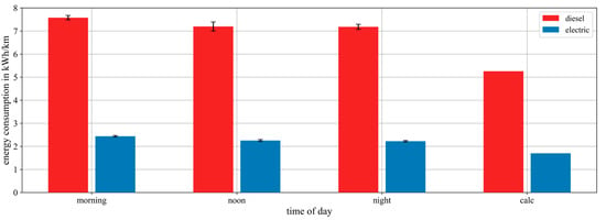
Figure 7.
Deviation of energy consumption for two types of propulsion (diesel in red, electric in blue) at different times of day and according to traffic flows, compared to calculated estimates (calc).
Overall, the simulated results are approximately 30% higher than the literature values for urban traffic, which can be attributed to several factors relevant for real-time routing applications, such as the overestimation of the acceleration behavior within the model [38], spacing intervals of stops, and condition-specific characteristics of the data from the literature [46].
3.2.2. TTW Emissions Related to Passenger Load
To assess the passenger impact on the environmental performance of bus services, specific emissions per passenger-kilometer were measured across morning, noon, and night scenarios at 17% occupancy. Figure 8 illustrates the comparison between these scenarios (with 17% occupancy representative of the German average) and the corresponding value from the literature for urban bus traffic emissions in Germany (as fleet mix value) from the German Environmental Agency (Umweltbundesamt), abbreviated as UBA in the plot [50]. The UBA value for CO2 is published as CO2-eq, taking into account other greenhouse gases; their amount in the case of this study is very low, and therefore the difference is negligible. The UBA-values are thus comparable with the SUMO values for the purpose of this analysis [46]. The variability is calculated between individual buses within a simulation scenario and between different times of day. The standard deviation within each scenario is below 3%, except for PM at noon, which is slightly higher but still below 5%. Across scenarios, the values overlap within the standard deviation ranges, except for CO2 in the morning scenario, which shows a distinct increase. The CO2 emissions vary moderately with time of day (mean value: 75.27 ± 2.32 g/Pkm, equals 1919 ± 59 g/km), and exceed the UBA reference only in the morning scenario. In contrast, the resulting NOx (mean value: 0.027 ± 0.005 g/Pkm, equals 0.71 ± 0.01 g/km) and PM (mean value: 0.0021 ± 0.0001 g/Pkm, equals 0.053 ± 0.002 g/km) from PHEMlight are considerably lower.
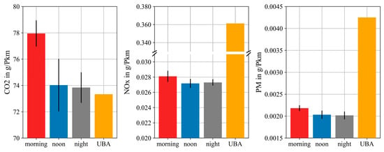
Figure 8.
Simulated TTW emissions of diesel Euro VI buses as a function of time of day for an occupancy of 17%, including the literature value as a comparison benchmark (Note: In the case of CO2, the UBA value is equal to CO2-equivalent emissions) [50].
Reported TTW values vary widely in the literature, depending on the methodology and data source: CO2 from about 900 to 1400 g/km, NOx from 0.04 to 2 g/km, and PM from 0.0001 to 0.08 g/km [11,17,24,25,46,50]. These deviations reflect differences in test procedures (PEMS, chassis dynamometer, or modeling), driving profiles, and emission standards. Compared to these studies, the simulated results in this work represent the lower range of modern Euro VI diesel buses.
The comparatively higher UBA values for NOx and PM can be explained by their aggregation over mixed fleets including various bus categories, Euro classes, and propulsion systems [50]. Additionally, UBA accounts for cold-start and idling effects as well as varying exhaust-after-treatment performance under real-world conditions, whereas PHEMlight represents an idealized, technology-specific case [47]. Hence, the model results indicate the lower bound of the emission ranges from the published literature on well-maintained Euro VI diesel buses, while UBA values capture the variability and degradation effects of the in-use fleet. The CO2 value of the UBA falls within the standard deviation range of the noon and night scenarios but is slightly lower than that of the morning scenario. In the morning, traffic is more congested, leading to lower speeds and longer travel times (see Section 3.1.2).
Since the modeled emissions fall within the value range of real-world observations, the noon scenario is taken as a representative operating condition to assess the passenger load threshold at which public bus transport becomes environmentally advantageous over individual car use. Therefore, the average emissions along the test route are plotted against passenger load in percent, with 100% corresponding to 150 passengers for the noon scenario of a single bus (Figure 9). As a reference, the UBA literature value for private car tank-to-wheel emissions is shown as a threshold (yellow line), representing an aggregated average (meaning, no differentiation between urban and long-distance trips) [50].
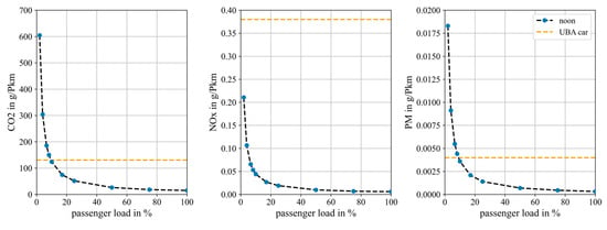
Figure 9.
Emissions (CO2, NOx, and PM) in g/Pkm against passenger load for diesel Euro VI buses. Modeled occupancy values marked in blue, supplemented by a black dashed trend line and the UBA emission values for aggregated average TTW car emissions as a dashed yellow line [50].
The per capita emissions show an exponential decay with increasing occupancy. The intersection with the private car threshold occurs between 9 and 10% occupancy for the route studied and operating conditions for CO2 and PM, whereas the UBA-value for NOx exceeds all modeled values. Considering that inner-city car emissions are typically higher due to frequent acceleration and deceleration, and because average velocities are often below 50 km/h (outside the optimum efficiency for combustion engine cars), even occupancy rates below 9% could be environmentally advantageous when using the bus within the test scope of this study. However, a caveat remains in that the model does not take into account particulate emissions from tire abrasion and brakes, and hence underestimates the PM values.
Test trips conducted throughout the day in Osnabrück indicated a decline in occupancy, with noticeably fewer passengers in the evening, although this observation is qualitative and not statistically validated. The literature, however, shows similar tendencies for public transport with higher occupancy during peak hours and a decrease at night [51,52]. The values obtained were below 7% occupancy, which approaches the range where the environmental benefit of the bus compared to the car diminishes. This underlines the importance of considering adaptive bus capacities or measures to increase the attractiveness of bus travel to maintain emission advantages over individual car use.
3.2.3. Emissions over Test Route
To assess the need for localized emission calculations in real-time routing evaluation, the emission values were recorded along the entire bus route to provide a spatial representation and to identify points with particularly high emission behavior, assuming 17% passenger occupancy. Figure 10 presents a comprehensive analysis of emission patterns (in g/km) and speed trajectories along the test route for all three times of day. Red coloring represents morning, blue for noon, and gray for night. The figure is structured in four rows, providing spatial perspectives on the speed trajectories and emission characteristics. The data portrays the mean profile with the corresponding standard deviation band calculated from the six buses for each time-of-day scenario. The fifth row, divided into four columns, shows the aggregated values for speed, CO2, NOx, and PM by speed zone. Zones 1 and 7 have a 50 km/h speed limit, Zones 2, 4, and 6 have a maximum speed of 30 km/h, while Zones 3 and 5 are pedestrian zones. In the speed trajectory subplot, 30 km/h zones are marked in red, and pedestrian zones are highlighted in blue. In the case of the emission plots, vertically dashed lines separate the zones.
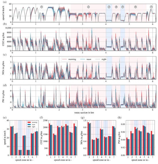
Figure 10.
Calculated emission profiles of diesel Euro VI buses. Background coloring marks speed limit zones, with red marking 30 km/h zones and blue marking pedestrian zones. (a) Speed trajectory with corresponding speed limit zones numbered in the plot. The numbers are also valid for plots b to d. (b) CO2, (c) NOx, and (d) PM emissions against the route sections for the three traffic flow scenarios. The last row (e–h) shows the aggregated values for speed, CO2, NOx, and PM emissions for each speed limit zone, the numbers correspond to the markings in (a).
The speed trajectories show characteristic acceleration and deceleration patterns at specific points along the route, indicating the locations of bus stops and traffic light systems. The behavior remains consistent across all three times of day for the initial 1.4 km section of the route. Beyond this point, the speed deviation between individual stops increases slightly, possibly corresponding with reaching the inner city ring, where traffic increases. However, the speed curves remain within the standard deviation bounds of each other, with only minor exceptions in isolated sections. The emission patterns closely follow the speed trajectory characteristics, exhibiting pronounced peaks during acceleration phases following stops and approaching zero emissions during deceleration periods. This relationship demonstrates the strong correlation between driving dynamics and instantaneous emission rates in urban bus operations.
The trajectory behavior within the speed zones can be categorized as follows: Zones 1 and 7 have a 50 km/h speed limit and mostly consist of varying speeds, with many acceleration and deceleration trajectories. Zones 2, 4, and 6 have a 30 km/h speed limit and have larger sections of constant speed, interspersed with halts. However, Zone 4 has both properties in equal measure. Zones 3 and 5 are pedestrian zones and are typified by constant speeds.
Overall, the high traffic morning scenario exhibits slightly elevated values across all emission types, with a few exceptions, corresponding to the lower average speeds observed during this period. For CO2 emissions, Zones 2 and 6 display the lowest emission rates, corresponding to 30 km/h zones, presumably due to constant speeds with minimal stop-and-go behavior. Notably, the pedestrian zone shows CO2 emission levels comparable to those observed in the 50 km/h zone and exceeding them. This could be because lower speeds are not optimal for motor efficiency. Interestingly, this effect seems to dominate over the acceleration and deceleration events occurring in the 30 km/h and 50 km/h zones.
NOx emissions follow a slightly different trend, with the highest emission values occurring in the 50 km/h speed limit zones, followed by Zone 4 (max. speed 30 km/h). Zone 1, for instance, produces more than double the NOx emissions compared to Zone 2 (30 km/h maximum), indicating that deceleration and acceleration dominate the overall velocity in the case of NOx. PM emissions demonstrate no clear correlation with maximum speed limits. The pedestrian zone (Zone 5) shows the highest PM emissions at over 0.07 g/km.
4. Discussion
This study aimed to evaluate the feasibility and practical relevance of emission-aware routing for urban bus systems by using a case study based on Osnabrück’s M5 bus route. It does so by applying a simulation model that uses historical traffic data and bus trajectories to replicate the real-world driving behavior of urban bus services in Osnabrück city. Validation results confirmed that the simulation model closely reflects real-world conditions, particularly in terms of bus trajectories and vehicle count data. The findings highlight the influence of various operational parameters, such as traffic flow and emission modeling choices, on the accuracy and relevance of emission estimates for routing applications.
The comparison of emission models revealed that the CO2 values generated using both the HBEFA-based and PHEMlight models were higher than those reported in the standard literature. This discrepancy is likely due to the route-specific scope of this study, consisting of frequent stop-and-go operations and short cruising phases, which highlights the importance of considering the influence of study area characteristics for spatial emission assessments. Additionally, the CO2 emissions from diesel propulsion in this study varied by up to 10% depending on the selected PHEMlight settings, highlighting both the model’s adaptability and the importance of careful calibration for reliable, scenario-specific emission assessment. However, limitations in PM and NOx estimations were identified, as tire abrasion and other non-exhaust sources were not considered in the models used. Accordingly, the absolute emission levels should be interpreted as case-specific, whereas the relative differences across traffic scenarios, modeling choices, and operational parameters are most relevant for routing-oriented applications.
As expected, electric buses showed lower energy consumption compared to diesel-powered buses, with the electric propulsion system resulting in around 70% lower consumption. However, while electric buses perform better overall, they still behave slightly differently under varying traffic conditions. This difference needs to be considered when developing routing applications that incorporate both diesel and electric propulsion systems into the public transport engine mix, accounting for both tank-to-wheel and well-to-tank perspectives.
Taking a range of passenger occupancy levels into account, this study shows that commuting by public bus with diesel propulsion produces less per capita emissions than private vehicle usage for occupancy rates above 10%. Therefore, in accordance with passenger occupancy levels reported in the literature, using the bus on average produces fewer TTW emissions during the day. When upstream processes are considered, the break-even point will probably shift so that even lower occupancies are preferable. Furthermore, CO2 emissions are only one impact factor in sustainable transport. By also considering other factors, such as land use, public transport can be more sustainable than private commuting, even when passenger loads are lower [50].
Spatially resolved emission trajectories further revealed the influence of acceleration-deceleration events and speed zones on the particle emissions. CO2, NOx, and PM emissions in particular exhibited a value variation of up to 50% depending on the speed zone. The findings suggest that speed zones, particularly lower-speed zones, have a significant impact on emissions on the exemplary bus route, highlighting the need for spatially resolved emission estimates in future routing applications.
Regarding temporal variations, differences between the traffic flow at different times of day were less pronounced than initially expected. Noon and night scenarios showed almost identical mean emission levels, whereas morning values were slightly elevated by 5%. This can be attributed to several factors: First, the SUMO traffic simulation employs optimized routing algorithms that may underrepresent extreme congestion scenarios compared to real-world conditions. Second, the sensor data used for calibration captured average operational conditions over the measurement period but may not have included rare high-congestion events, potentially limiting the observed variance. Nevertheless, this finding remains valuable for routing applications targeting normal operating conditions, which represent most user interactions.
Study Limitations
While the study provides valuable insights into emission patterns on an exemplary bus route in Osnabrück, there are several limitations that should be noted:
- Route representativeness: The bus route studied cannot be considered fully representative of all urban bus operations. While it does capture typical features such as stop spacing, speed limits, and traffic heterogeneity, the specific route characteristics may not fully reflect the variety of urban traffic conditions.
- Traffic conditions: The traffic conditions modeled in this study are somewhat homogeneous across the scenarios, which could limit the broader applicability of the results. To better reflect real-world variability, further studies should account for more diverse traffic patterns and incorporate a broader spectrum of operational conditions.
- Model Limitations: The PHEMlight model used in this study has limitations, particularly in its failure to account for real-world factors such as tire abrasion, wear effects, and cold-start emissions. These factors could significantly influence NOx and PM estimates, and future iterations of the model should integrate these aspects to enhance the accuracy of the emissions predictions.
- Idealized Vehicle State: The assumption of a well-maintained fleet in the simulation does not fully account for operational variability, fleet degradation, and maintenance issues, all of which need to be considered in future real-world applications to improve the robustness and reliability of the emission estimates.
5. Conclusions and Outlook
This study establishes a framework for emission-aware routing in urban bus systems. While the scope of this research is limited, a number of key recommendations can be derived for future routing applications.
To ensure more accurate emission calculations, emission-aware routing implementation on digital mobility services should rely on route-specific traffic dynamics and local fleet data rather than general literature values. This includes adapting the engine mix and considering variations in passenger load to enhance accuracy and provide meaningful and context-sensitive emission feedback. Further, the analysis highlights that different pollutants exhibit distinct sensitivity to traffic conditions and speed profiles. This underscores that “eco-friendly” routing can be defined by multiple impact categories, depending on the environmental priorities and exposure characteristics of a given urban area.
From a modeling perspective, future work should extend the emission assessment to more diverse traffic situations, including explicitly congested conditions, and evaluate the robustness of the findings across a larger set of bus routes or entire urban networks. Systematic comparisons of emission modeling approaches and targeted sensitivity analyses would further support informed decisions about model granularity in routing applications. For practical implementation, emission-aware routing systems should be embedded in city-specific digital mobility platforms, where real-time or near-real-time traffic data, such as detector-based measurements, can be used to dynamically adjust routing recommendations. When scaled to a network level, traffic simulation, in combination with real-time traffic data, could provide additional value for urban planners by supporting the identification of high-emission zones, evaluating mitigation strategies, and informing long-term transport planning within a digital-twin framework.
Beyond technical aspects, behavioral and psychological factors represent an important avenue for future research. Investigating how emission information is communicated to users, what level of detail is understandable and actionable, and how different visualization strategies influence travel behavior and modal choice will be crucial for achieving actual emission reductions through routing-based interventions.
Author Contributions
Conceptualization, R.K., S.-M.A., M.H. and S.R.; methodology, R.K., S.-M.A., M.H. and S.R.; software, R.K., S.-M.A. and M.H.; validation, R.K., S.-M.A., M.H. and S.R.; formal analysis, R.K. and S.-M.A.; investigation, R.K. and S.-M.A.; resources, S.R.; data curation, R.K. and S.-M.A.; writing—original draft preparation, R.K.; writing—review and editing, R.K., S.-M.A., M.H. and S.R.; visualization, R.K. and S.-M.A.; supervision, M.H. and S.R.; project administration, S.R.; funding acquisition, S.R. All authors have read and agreed to the published version of the manuscript.
Funding
This research was funded by the Federal Ministry of Research, Technology, and Space (BMFTR), grant number 16SV8948.
Institutional Review Board Statement
Not applicable.
Informed Consent Statement
Not applicable.
Data Availability Statement
The data that support the findings of this study are available from the corresponding author upon reasonable request. The data are not publicly available due to privacy.
Acknowledgments
The authors thank the City of Osnabrück for providing access to the TEU data and granting permission for publication. During the preparation of this manuscript, the authors used Chat GPT 5 mini and Claude Sonnet 4 R for the purposes of text generation, editing, and support in analysis prior to professional language editing. The authors have reviewed and edited the output and take full responsibility for the content of this publication.
Conflicts of Interest
The authors declare no conflicts of interest.
Abbreviations
The following abbreviations are used in this manuscript:
| GHG | Greenhouse gas emissions |
| LAD | Lane area detector |
| TEU | Traffic eye universal |
| TLS | Traffic light system |
| TTW | Tank-to-wheel |
| UBA | Umweltbundesamt (German Environmental Agency) |
References
- Edenhofer, O.; Pichs-Madruga, R.; Sokona, Y.; Farahani, E.; Kadner, S.; Seyboth, K.; Adler, A.; Baum, I.; Brunner, S.; Eickemeier, P.; et al. IPCC, 2014: Climate Change 2014: Mitigation of Climate Change. Contribution of Working Group III to the Fifth Assessment Report of the Intergovernmental Panel on Climate Change; Cambridge University Press: Cambridge, UK; New York, NY, USA, 2014. [Google Scholar]
- Umweltbundesamt. Treibhausgas-Emissionen in Deutschland. Available online: https://www.umweltbundesamt.de/daten/klima/treibhausgas-emissionen-in-deutschland#emissionsentwicklung (accessed on 23 July 2025).
- Umweltbundesamt. Fahrleistungen, Verkehrsleistung und Modal Split. Available online: https://www.umweltbundesamt.de/daten/verkehr/fahrleistungen-verkehrsaufwand-modal-split#undefined (accessed on 23 July 2025).
- Christou, A.; Giechaskiel, B.; Olofsson, U.; Grigoratos, T. Review of Health Effects of Automotive Brake and Tyre Wear Particles. Toxics 2025, 13, 301. [Google Scholar] [CrossRef] [PubMed]
- Krzyzanowski, M.; Kuna-Dibbert, B.; Schneider, J. Health Effects of Transport-Related Air Pollution; World Health Organization Europe: Copenhagen, Denmark, 2005; ISBN 9289013737. [Google Scholar]
- Consilium. Fit for 55. Available online: https://www.consilium.europa.eu/en/policies/fit-for-55/ (accessed on 15 December 2025).
- European Commission. Transport and the Green Deal. Available online: https://commission.europa.eu/topics/transport-and-tourism/transport-and-green-deal_en (accessed on 15 December 2025).
- Routing Profiles–OpenStreetMap Wiki. Available online: https://wiki.openstreetmap.org/wiki/Routing_profiles#Efficient_driver (accessed on 5 December 2025).
- Use Eco-Friendly Routes on Your Google Maps App-Android-Google Maps Help. Available online: https://support.google.com/maps/answer/11470237?hl=en&co=GENIE.Platform%3DAndroid (accessed on 5 December 2025).
- ISO 14083:2023; Greenhouse Gases—Quantification and Reporting of Greenhouse Gas Emissions Arising from Transport Chain Operations. ISO: Geneva, Switzerland, 2023. Available online: https://www.iso.org/standard/78864.html (accessed on 7 January 2026).
- Perdikopoulos, M.; Karageorgiou, T.; Ntziachristos, L.; Deville Cavellin, L.; Joly, F.; Vigneron, J.; Arfire, A.; Debert, C.; Sanchez, O.; Gaie-Levrel, F.; et al. Developing Emission Factors from Real-World Emissions of Euro VI Urban Diesel, Diesel-Hybrid, and Compressed Natural Gas Buses. Atmosphere 2025, 16, 293. [Google Scholar] [CrossRef]
- Wei, T.; Frey, H.C. Factors affecting variability in fossil-fueled transit bus emission rates. Atmos. Environ. 2020, 233, 117613. [Google Scholar] [CrossRef]
- Nylund, N.-O.; Söderena, P.; Mäkinen, R.; Anttila, T. On route to clean bus services. In Proceedings of the TRA2020, the 8th Transport Research Arena: Rethinking Transport—Towards Clean and Inclusive Mobility, Helsinki, Finland, 27–30 April 2020; p. 12. [Google Scholar]
- López, J.M.; Flores, N.; Jiménez, F.; Aparicio, F. Emissions Pollutant from Diesel, Biodiesel and Natural Gas Refuse Collection Vehicles in Urban Areas. In Highway and Urban Environment; Rauch, S., Ed.; Springer: Dordrecht, The Netherlands, 2009; pp. 141–148. ISBN 978-90-481-3043-6. [Google Scholar]
- Westerdahl, D.; Wang, X.; Pan, X.; Zhang, K.M. Characterization of on-road vehicle emission factors and microenvironmental air quality in Beijing, China. Atmos. Environ. 2009, 43, 697–705. [Google Scholar] [CrossRef]
- Wang, J.; Xu, F.; Chen, X.; Li, J.; Wang, L.; Jiang, B.; Chen, Y. Study on the Emission Characteristics of Typical City Buses under Actual Road Conditions. Atmosphere 2024, 15, 148. [Google Scholar] [CrossRef]
- Gis, M. Comparative studies exhaust emissions of the Euro VI buses with diesel engine and spark-ignition engine CNG fuelled in real traffic conditions. MATEC Web Conf. 2017, 118, 7. [Google Scholar] [CrossRef]
- Hossain, M.R.; Hasan, M.H.; Yu, H.; Abou-Senna, H.; Brandin, T.; Gladwin, K. Macroscopic and Microscopic Emissions Modeling for Alternative Fuel Transit Buses: Route-Specific Operational and Environmental Performance Analysis. SSRN 2025. [Google Scholar] [CrossRef]
- López-Martínez, J.M.; Jiménez, F.; Páez-Ayuso, F.J.; Flores-Holgado, M.N.; Arenas, A.N.; Arenas-Ramirez, B.; Aparicio-Izquierdo, F. Modelling the fuel consumption and pollutant emissions of the urban bus fleet of the city of Madrid. Transp. Res. Part D Transp. Environ. 2017, 52, 112–127. [Google Scholar] [CrossRef]
- Shan, X.; Chen, X.; Jia, W.; Ye, J. Evaluating Urban Bus Emission Characteristics Based on Localized MOVES Using Sparse GPS Data in Shanghai, China. Sustainability 2019, 11, 2936. [Google Scholar] [CrossRef]
- Hasan, U.; Whyte, A.; AlJassmi, H. A Microsimulation Modelling Approach to Quantify Environmental Footprint of Autonomous Buses. Sustainability 2022, 14, 15657. [Google Scholar] [CrossRef]
- Yu, Q.; Li, T.; Li, H. Improving urban bus emission and fuel consumption modeling by incorporating passenger load factor for real world driving. Appl. Energy 2016, 161, 101–111. [Google Scholar] [CrossRef]
- Diaz, J.; Pérez, B.; Fernández, F.J. Energy Assessment of Alternative City Bus Lines: A Case Study in Gijón, Spain. Sustainability 2024, 16, 4101. [Google Scholar] [CrossRef]
- Miraftabzadeh, S.M.; Saldarini, A.; Cattaneo, L.; El Ajami, S.; Longo, M.; Foiadelli, F. Comparative analysis of decarbonization of local public transportation: A real case study. Heliyon 2024, 10, e25778. [Google Scholar] [CrossRef] [PubMed]
- Szumska, E.; Pawełczyk, M.; Pistek, V. Evaluation of the Life Cycle Costs for urban buses equipped with conventional and hybrid drive trains. Arch. Automot. Eng.–Arch. Motoryz. 2019, 83, 73–86. [Google Scholar] [CrossRef]
- Vieira, J.P.B.; Pereira, R.H.; Andrade, P.R. Estimating public transport emissions from General Transit Feed Specification data. Transp. Res. Part D Transp. Environ. 2023, 119, 103757. [Google Scholar] [CrossRef]
- Chen, X.; Shan, X.; Ye, J.; Yi, F.; Wang, Y. Evaluating the Effects of Traffic Congestion and Passenger Load on Feeder Bus Fuel and Emissions Compared with Passenger Car. Transp. Res. Procedia 2017, 25, 616–626. [Google Scholar] [CrossRef]
- URBANIST—Miteinander Durch Innovation. Available online: https://www.interaktive-technologien.de/projekte/urbanist (accessed on 18 September 2025).
- netedit-SUMO Documentation. Available online: https://sumo.dlr.de/docs/Netedit/index.html (accessed on 15 December 2025).
- Stadtwerke Osnabrück. E-Busse. Available online: https://www.stadtwerke-osnabrueck.de/swo-mobil/bus/elektrobusse (accessed on 18 September 2025).
- VDL Bus & Coach bv. Data Sheet. Available online: https://www.vdlbuscoach.com/en/products/citea/new-generation-citeas (accessed on 5 September 2025).
- Man. Man Lion’s City 18-Technical Data Sheet. Available online: https://www.man.eu/de/de/bus/der-man-lion_s-city/technik-und-spezifikation/alle-modelle-und-spezifikationen.html (accessed on 19 September 2025).
- Devunuri, S.; Lehe, L.J.; Qiam, S.; Pandey, A.; Monzer, D. Bus stop spacing statistics: Theory and evidence. J. Public Transp. 2024, 26, 100083. [Google Scholar] [CrossRef]
- Poelman, H.; Dijkstra, L.; Ackermans, L. How Many People Can You Reach by Public Transport, Bicycle or on Foot in European Cities? Measuring Urban Accessibility for Low-Carbon Modes; Publications Office of the European Union: Luxembourg, 2020; ISBN 978-92-76-10253-3. [Google Scholar]
- HBEFA-Based-SUMO Documentation. Available online: https://sumo.dlr.de/docs/Models/Emissions/HBEFA-based.html (accessed on 28 October 2025).
- OSMWebWizard-SUMO Documentation. Available online: https://sumo.dlr.de/docs/Tutorials/OSMWebWizard.html (accessed on 8 December 2025).
- Definition of Vehicles, Vehicle Types, and Routes-SUMO Documentation. Available online: https://sumo.dlr.de/docs/Definition_of_Vehicles%2C_Vehicle_Types%2C_and_Routes.html#car-following_model_parameters (accessed on 8 December 2025).
- Wagner, P.; Erdmann, J. SUMO’s Interpretation of the Krauß Model. SUMO Conf. Proc. 2025, 6, 17–24. [Google Scholar] [CrossRef]
- HBEFA4-Based-SUMO Documentation. Available online: https://sumo.dlr.de/docs/Models/Emissions/HBEFA4-based.html (accessed on 29 July 2025).
- Graz, R.I.T. PHEMlight. Available online: https://www.itna.tugraz.at/en/research/areas/em/simulation/phemlight.html (accessed on 5 September 2025).
- Allekotte, M.; Biemann, K.; Colson, M.; Heidt, C.; Kräck, J.; Knörr, W. Aktualisierung TREMOD/TRE-MOD-MM und Ermittlung der Emissionsdaten des Verkehrs nach KSG im Jahr 2023: Endbericht; Umweltbundesamt: Dessau-Roßlau, Germany, 2024.
- de Filippo, G.; Marano, V.; Sioshansi, R. Simulation of an electric transportation system at The Ohio State University. Appl. Energy 2014, 113, 1686–1691. [Google Scholar] [CrossRef]
- Wu, J.; Kulcsár, B.; Selpi; Qu, X. A modular, adaptive, and autonomous transit system (MAATS): An in-motion transfer strategy and performance evaluation in urban grid transit networks. Transp. Res. Part A Policy Pract. 2021, 151, 81–98. [Google Scholar] [CrossRef]
- Meibom, P. Technology Analysis of Public Transport Modes: Byg Rapport No. R-022; Technical University of Denmark: Lyngby, Denmark, 2002. [Google Scholar]
- IPCC. 2006 IPCC Guidelines for National Greenhouse Gas Inventories; Energy; Eggleston, S., Buendia, L., Miwa, K., Ngara, T., Tanabe, K., Eds.; Institute for Global Environmental Strategies (IGES): Hayama, Japan, 2006; Volume 2, ISBN 4-88788-032-4. [Google Scholar]
- Söderena, P.; Nylund, N.-O.; Mäkinen, R. City Bus Performance Evaluation; VTT Customer Report No. VTT-CR-00544-19; VTT Technical Research Centre of Finland: Espoo, Finland, 2019. [Google Scholar]
- PHEMlight5-SUMO Documentation. Available online: https://sumo.dlr.de/docs/Models/Emissions/PHEMlight5.html (accessed on 20 October 2025).
- German Aerospace Center (DLR) and Others. Why Vehicles Are Teleporting-SUMO Documentation. Available online: https://sumo.dlr.de/docs/Simulation/Why_Vehicles_are_teleporting.html (accessed on 18 September 2025).
- Bundesministerium für Wirtschaft und Klimaschutz. Begleituntersuchung zur Förderung von Elektrobussen im ÖPNV: Eine Bilanz der Förderrichtlinie zur Anschaffung von Elektrobussen im Öffentlichen Personennahverkehr für die Jahre 2018 bis 2023–im Auftrag des Bundesministeriums für Wirtschaft und Klimaschutz (BMWK); Bundesministerium für Wirtschaft und Klimaschutz: Berlin, Germany, 2024.
- Allekotte, M.; Althaus, H.-J.; Bergk, F.; Biemann, K.; Knörr, W.; Sutter, D. Umweltfreundlich Mobil!: Ein Ökologischer Verkehrsartenvergleich für den Personen-und Güterverkehr in Deutschland; Umweltbundesamt: Dessau-Roßlau, Germany, 2020. Available online: https://www.umweltbundesamt.de/publikationen (accessed on 17 March 2025).
- Luo, D.; Bonnetain, L.; Cats, O.; van Lint, H. Constructing Spatiotemporal Load Profiles of Transit Vehicles with Multiple Data Sources. Transp. Res. Rec. J. Transp. Res. Board 2018, 2672, 175–186. [Google Scholar] [CrossRef]
- Roncoli, C.; Chandakas, E.; Kaparias, I. Estimating on-board passenger comfort in public transport vehicles using incomplete automatic passenger counting data. Transp. Res. Part C Emerg. Technol. 2023, 146, 103963. [Google Scholar] [CrossRef]
Disclaimer/Publisher’s Note: The statements, opinions and data contained in all publications are solely those of the individual author(s) and contributor(s) and not of MDPI and/or the editor(s). MDPI and/or the editor(s) disclaim responsibility for any injury to people or property resulting from any ideas, methods, instructions or products referred to in the content. |
© 2026 by the authors. Licensee MDPI, Basel, Switzerland. This article is an open access article distributed under the terms and conditions of the Creative Commons Attribution (CC BY) license.