


Abstract
Microseismic monitoring is extensively applied in hydraulic fracturing and mineral extraction, with accurate event localization being a critical component. Recently, deep learning approaches have shown promise for microseismic event localization; however, most of these supervised methods depend on large, labeled datasets, which are costly and challenging to acquire. To mitigate this issue, we propose a semi-supervised approach based on a residual convolutional autoencoder (RCAE) for automated microseismic localization, designed to leverage limited labeled data effectively and improve source localization accuracy even with small sample sizes. Our method employs pre-training by masking and reconstructing unlabeled seismic records, while integrating residual connections within the encoder to enhance feature extraction from seismic signals. This enables high localization accuracy with minimal labeled data, resulting in significant cost savings. Experimental results indicate that our method surpasses purely supervised approaches on both a 2D salt dome model and a 3D homogeneous half-space model, validating its effectiveness in microseismic localization. Further comparisons with baseline models highlight the method’s advantages, providing an innovative solution for improving cost-efficiency in practical applications.
1. Introduction
Monitoring technology uses receivers to detect seismic signals generated by rock fractures, extracting relevant microseismic information for real-time monitoring of subsurface conditions and production activities. This technology is widely applied in mineral extraction and hydraulic fracturing [1,2], where precise microseismic localization plays a crucial role. By determining the exact location of underground microseismic sources, it aids in tracking rock mass fractures and monitoring crack propagation. In mineral extraction, microseismic localization assesses the stability and fracture trends of the rock mass, providing scientific support for safe operations [3]. In hydraulic fracturing, it evaluates the effectiveness of fracturing and the direction of crack extension, facilitating optimization of extraction strategies [4]. Accurate microseismic source localization also enables rapid risk assessment and the implementation of safety measures, thereby enhancing both safety and production efficiency.
Given the importance of microseismic localization, researchers have developed a range of localization algorithms. Among travel-time-based methods, the most notable include Geiger’s least-squares linear localization algorithm [5], Waldhauser’s double-difference method [6], and nonlinear approaches such as the Powell algorithm [7], grid search [8,9], and genetic algorithm [10]. In recent years, waveform-based migration methods have also been widely applied, including source imaging through waveform inversion [11,12], amplitude-based source scanning [13,14], and reverse time migration methods that eliminate the need for travel-time picking [15,16,17]. Most of these traditional localization methods rely on seismic wave propagation principles within subsurface media. However, they generally require substantial computational resources, which limits their feasibility for real-time automatic localization.
In recent years, the rapid advancement of deep learning has led to promising applications of neural networks in seismic localization. Perol et al. [18] introduced the ConvNetQuake model for seismic detection and localization. Building on this work, Bai et al. [19] developed and trained a Long Short-Term Memory Fully Convolutional Network model, achieving further improvements in detection and localization accuracy. Kriegerowski et al. [20] bypassed region-based predictions by using a Convolutional Neural Network (CNN) to directly predict the three-dimensional coordinates of the seismic source. Van et al. [21] used a Graph Convolutional Network by normalizing seismic events and station locations, incorporating station latitude and longitude as network inputs, to achieve precise source localization. Wamriew et al. [22] designed a joint inversion CNN model capable of simultaneously estimating source location and the velocity model. Feng et al. [23] applied deep reinforcement learning to frame the source localization task as a Markov Decision Process, enabling an agent to learn optimal microseismic source localization strategies with notable success. Zhang et al. [24] trained a CNN using early real data from Oklahoma to detect new microseismic events. Additionally, Wang et al. [25] and Vinard et al. [26] employed forward modeling based on field-specific velocity models at hydraulic fracturing sites in Oklahoma and Texas, respectively. By training CNN and U-Net models with synthetic data, they successfully localized microseismic events based on real seismic data, underscoring the applicability and effectiveness of neural networks in real production environments.
However, these methods are all based on supervised learning, and their localization performance depends heavily on large labeled datasets. In practical applications, obtaining accurate source locations is both challenging and costly, which significantly limits the broader adoption of these approaches. Consequently, achieving accurate localization with limited labeled data has become an urgent challenge.
To address this challenge, self-supervised learning has attracted increasing attention for its ability to perform pre-training on unlabeled data, extracting intrinsic features that improve the performance of subsequent tasks [27,28]. Currently, self-supervised learning approaches can be categorized into two main types: generative and contrastive. Generative methods learn data representations by predicting missing parts or reconstructing complete data and have been widely used in seismic data processing tasks, including denoising [29,30,31], interpolation [32,33,34], velocity modeling [35] and reconstruction [36]. In localization, Feng et al. [37] applied Generative Adversarial Networks to generate synthetic seismic data, enhancing feature extraction and improving localization accuracy even with only a small number of source labels. In contrast, contrastive methods learn effective feature representations by simultaneously maximizing the distinctions between different samples and the similarities of similar samples. Si et al. [38] proposed a seismic foundation model that pre-trains the network in this way, then freezes the pre-trained feature extractor for downstream seismic data processing tasks.
To take advantage of self-supervised learning and enhance the localization accuracy of microseismic events with limited labeled data, we propose a semi-supervised automatic localization method based on a residual convolutional autoencoder (RCAE). In the methodology section, during the self-supervised learning phase, we mask unlabeled seismic records and feed them into the network for reconstruction, pre-training the convolutional autoencoder. Residual connections are incorporated to strengthen the network’s feature extraction from seismic records. In the supervised learning phase, we use the pre-trained encoder, freezing its parameters, and add a convolutional network for the localization task, training with a small set of labeled seismic records. In the experimental section, we synthesize seismic records using a 3D homogeneous model and a 2D salt dome model to evaluate the proposed method. We compare results with those of purely supervised learning approaches. To ensure a fair comparison, we also include ResNet [39], commonly used in computer vision, and the CNN model by Wang et al. [25] as baseline models. In the discussion, we examined the effects of different masking ratios and labeled sample sizes on localization accuracy.
2. Materials and Methods
In this section, we describe the Residual Convolutional Autoencoder (RCAE) and the localization network structure used in this study, along with essential training details. We first discuss the design of the RCAE and its self-supervised learning process, followed by an overview of the convolutional network for microseismic event localization and the supervised learning implementation.
2.1. Residual Convolutional Autoencoder (Self-Supervised Learning Process)
Convolutional Autoencoder (CAE) is a neural network that combines the strengths of convolutional neural networks and autoencoders [40], making it well-suited for data with spatial features, such as images [41] and seismic waveforms [42,43,44]. The CAE encodes a compressed representation of the input data and reconstructs it through a decoder, allowing for unsupervised learning of data features without labeled data [45,46].
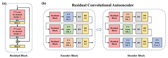
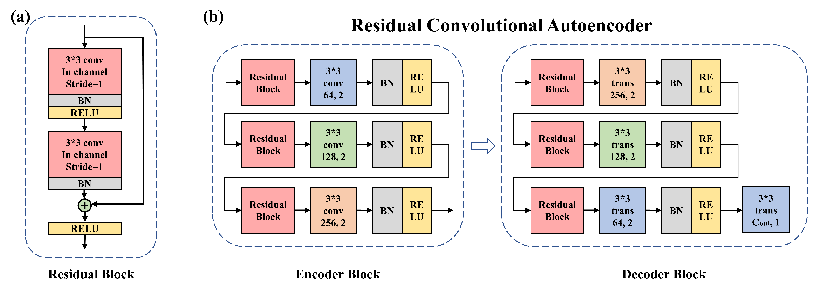
In this study, we integrate a residual structure into the CAE, inspired by ResNet, to address the common challenges of gradient vanishing and explosion in deep networks [47]. The residual structure consists of several residual blocks, as illustrated in Figure 1. Each block includes two convolutional layers, with batch normalization and ReLU activation function following each convolution. The ReLU (Rectified Linear Unit) activation function, defined as , introduces nonlinearity by suppressing negative activations while retaining positive responses, thereby improving training efficiency and mitigating gradient vanishing issues. Batch normalization accelerates convergence and reduces training instability due to shifts in layer input distributions, while ReLU introduces nonlinearity, enhancing the network’s ability to capture complex features. The core feature of each residual block is the skip connection, where the input bypasses the convolutional layers and directly connects to the output, effectively serving as an identity mapping. This design enables smooth gradient flow back to shallow layers, preserving critical information even in deep networks, which ensures stable and effective feature extraction. Additionally, the residual structure speeds up convergence and enhances training efficiency in deep networks [48].
Figure 1.
Architecture of RCAE: (a) Residual block structure: A basic unit composed of two sequential 3 × 3 convolutional layers (stride = 1) with batch normalization (BN) and ReLU activation, and a skip connection. (b) Overall RCAE framework: The encoder (left) uses residual blocks with 3 × 3 convolutions (stride = 2) to downsample feature maps, while the decoder (right) employs residual blocks with 3 × 3 transposed convolutions (stride = 2) for upsampling. The architecture enables masked reconstruction during pre-training.
The architecture of RCAE is shown in Figure 1, with the encoder and decoder as its core components, responsible for feature extraction and reconstruction of seismic records, respectively. Seismic data are first passed through the encoder, which consists of three residual blocks. Each block extracts features through convolution layers, with residual connections ensuring effective transmission of key information. As the network deepens, the encoder compresses the input data through successive convolutions and pooling layers, capturing low-dimensional representations such as vertex positions and curvature information, which are closely related to the source location. After feature extraction, these low-dimensional feature vectors are passed to the decoder. Like the encoder, the decoder is composed of residual blocks and progressively reconstructs these features to approximate the original seismic records through transposed convolution.
To fully leverage the unique properties of seismic data and extract meaningful features, we introduce a masking strategy to enhance the feature extraction capability of the RCAE. Considering that each seismic trace represents a fundamental structural unit, a trace-wise masking scheme is adopted, in which a subset of seismic traces within each record is randomly selected and entirely masked along the time axis. The masking ratio is defined as the proportion of masked traces relative to the total number of traces in a seismic record. This operation simulates realistic data incompleteness commonly encountered in seismic acquisition. By reconstructing the masked traces from the remaining observed data, the network is encouraged to learn robust and physically meaningful representations of seismic signals. As a result, the encoder becomes more adaptive to incomplete data during training and produces feature representations that generalize well for subsequent microseismic localization tasks.
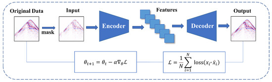
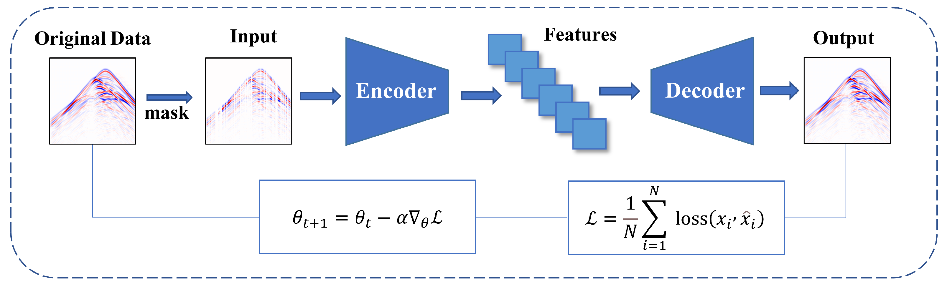
The overall training process for self-supervised learning in this study is shown in Figure 2.
Figure 2.
Self-supervised Learning Training Flowchart. Original seismic data are partially masked and fed into the encoder. Extracted features are decoded to reconstruct the input. Network parameters are updated by minimizing reconstruction loss, enabling self-supervised pre-training without labeled data.
The masked data reconstruction based on the RCAE can be expressed by the following equation:
where denotes the mapping of the model between masked data and complete data, where x represents the complete seismic data, denotes the masked version of x used as input, and represents the model parameters (weights and biases). The final reconstructed seismic data is represented by . We then apply an L2 norm-based loss function to measure the reconstruction error:
where N denotes the number of seismic data samples in a batch from the training set. We use the ADAM algorithm to optimize the parameters, with the process detailed as follows:
where and denote the network parameters before and after an update, respectively, is the learning rate, and represents the gradient of the loss function with respect to the parameters. After training, the optimal parameter set is obtained, minimizing the loss function. Thus, the final optimal reconstruction can be expressed as
Throughout the training process, no additional labels are introduced; instead, the data itself serves as its label. This training approach enables us to obtain an encoder capable of effectively extracting features from seismic records.
2.2. Localization Network (Supervised Learning Process)
In the self-supervised learning phase, the RCAE’s encoder gradually develops its ability to extract key features from seismic records by reconstructing masked seismic data. This process enables the encoder to capture the general characteristics of seismic data effectively, laying a strong foundation for the subsequent small-sample localization task.
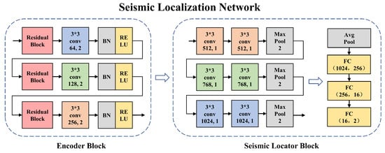
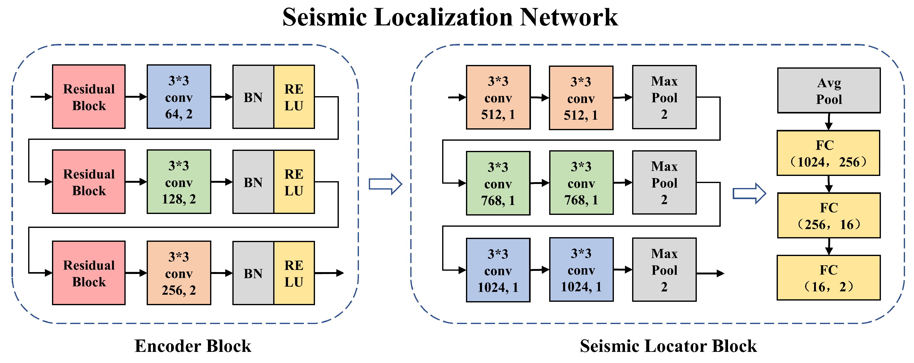
Building on this, we add a convolutional network after the encoder, specifically designed for localization. Figure 3 illustrates the architecture of the Seismic Localization Network (SLN). After self-supervised training, the encoder’s weights are frozen to serve as a feature extractor. The input seismic data first pass through the encoder, which extracts deep features containing source information. These features are then passed to the localization network, with the Seismic Locator Block in the figure detailing this structure. The localization network, composed of multiple convolutional and pooling layers, further processes the encoder-extracted features to refine high-level information relevant to the source location. Finally, through a fully connected layer, the model outputs the coordinates of the source location, completing the localization task.
Figure 3.
Architecture of SLN. The left part shows the encoder for extracting deep features from seismic signals. The right part is the locator block, which uses convolution, pooling, and fully connected layers to regress the source coordinates. This network is used for supervised source localization.
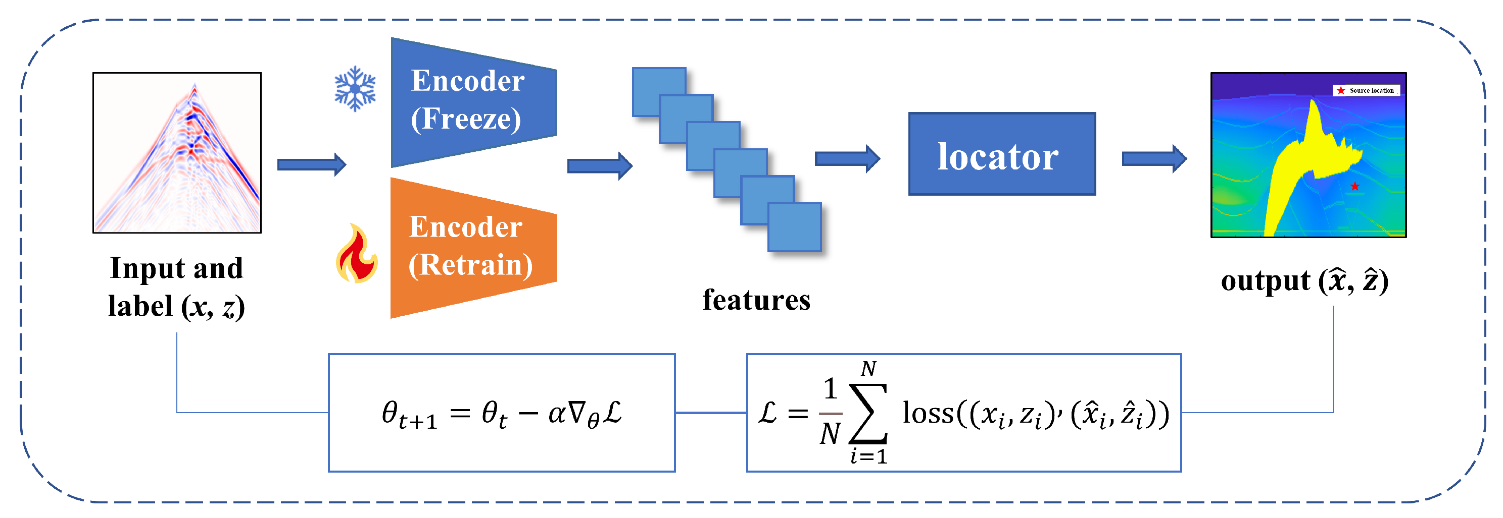
The effectiveness of this semi-supervised localization method is evaluated by comparison with a fully supervised strategy. In our method, the encoder undergoes pre-training through self-supervised learning, allowing it to acquire stable and robust seismic record features. Since only a limited amount of labeled data is available in the subsequent supervised learning stage, we freeze the encoder parameters to prevent overfitting and retain the general features extracted during the self-supervised phase. This strategy ensures that gradients propagate only within the localization module, without affecting the stable features already learned by the front-end encoder. By freezing the encoder, the subsequent small-sample supervised training focuses solely on fine-tuning the localization module (the network’s back end), thereby enhancing the model’s stability and generalization ability under small-sample conditions. In contrast, the fully supervised method trains the entire network from scratch, without using pre-trained parameters, covering both the encoder and the localization network. By comparing these two approaches (referred to as the Freeze strategy and the Retrain strategy), we can assess how much self-supervised pre-training improves source localization performance within the semi-supervised framework.
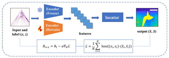
In the supervised learning phase, the training procedures for both strategies are illustrated in Figure 4. The input data consists of seismic signals, while the output is the predicted source coordinates . The source location corresponding to the seismic records is used as the target label. The target labels are used to compute the loss function and guide the model optimization process. The network parameters are iteratively adjusted by minimizing the error between the predicted and actual source locations. For the frozen strategy, only the localization network’s parameters are updated, whereas the retraining strategy involves updating all network parameters. The mean squared error (MSE) serves as the loss function to quantify the difference between predicted and actual coordinates, as given by the following equation:
where N is the sample size, and represent the true source coordinates, and and are the predicted coordinates. denotes the model parameters to be adjusted for each strategy, optimized using the ADAM algorithm.
Figure 4.
Supervised Learning Training Flowchart. The input is the seismic record, and the output is the predicted source coordinate ; the label is the corresponding true coordinate . The model is trained by minimizing the error between predictions and labels. The encoder modules are color-coded: blue for the freeze strategy (our proposed method), which uses a fixed pre-trained encoder and trains only the locator; orange for the retrain strategy, which trains the entire network from scratch.
3. Results
In the experimental phase, we tested using a 2D salt dome model and a 3D homogeneous half-space model. Using these models, we synthesized seismic records from various sources to build the dataset. Two training strategies were evaluated: the proposed semi-supervised method with a frozen pre-trained encoder (Freeze), and a fully supervised variant trained from scratch (Retrain), which serves as a control to quantify the benefits of pre-training. To evaluate the performance of the semi-supervised method more accurately, we introduced two different network architectures as baseline models. The first benchmark is a CNN-based microseismic localization model proposed by Wang and Alkhalifah (2022) [25], which employs multiple convolutional and pooling layers to extract features from seismic records, followed by fully connected layers to directly regress the source coordinates, and has been successfully applied to field microseismic data from the Arkoma Basin, Oklahoma. The second baseline is ResNet-18 [39], a representative deep residual network composed of 18 layers with identity skip connections, which is adopted as a standard supervised benchmark model for comparison in the microseismic localization task. Both baseline models perform source localization using supervised learning. To ensure fair comparisons, we used consistent hyperparameter settings, training data samples, and evaluated localization performance on the same test set across all four methods. Finally, we conducted a detailed analysis and discussion of each method’s localization results to compare model performance and applicability.
3.1. 2D Salt Dome Model
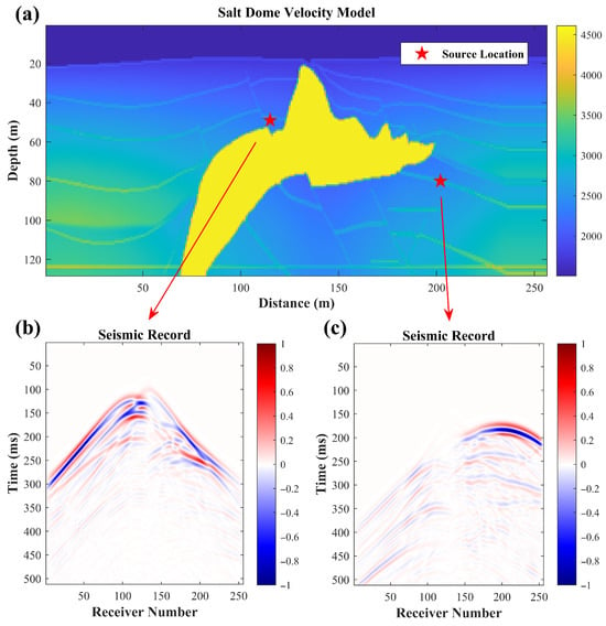
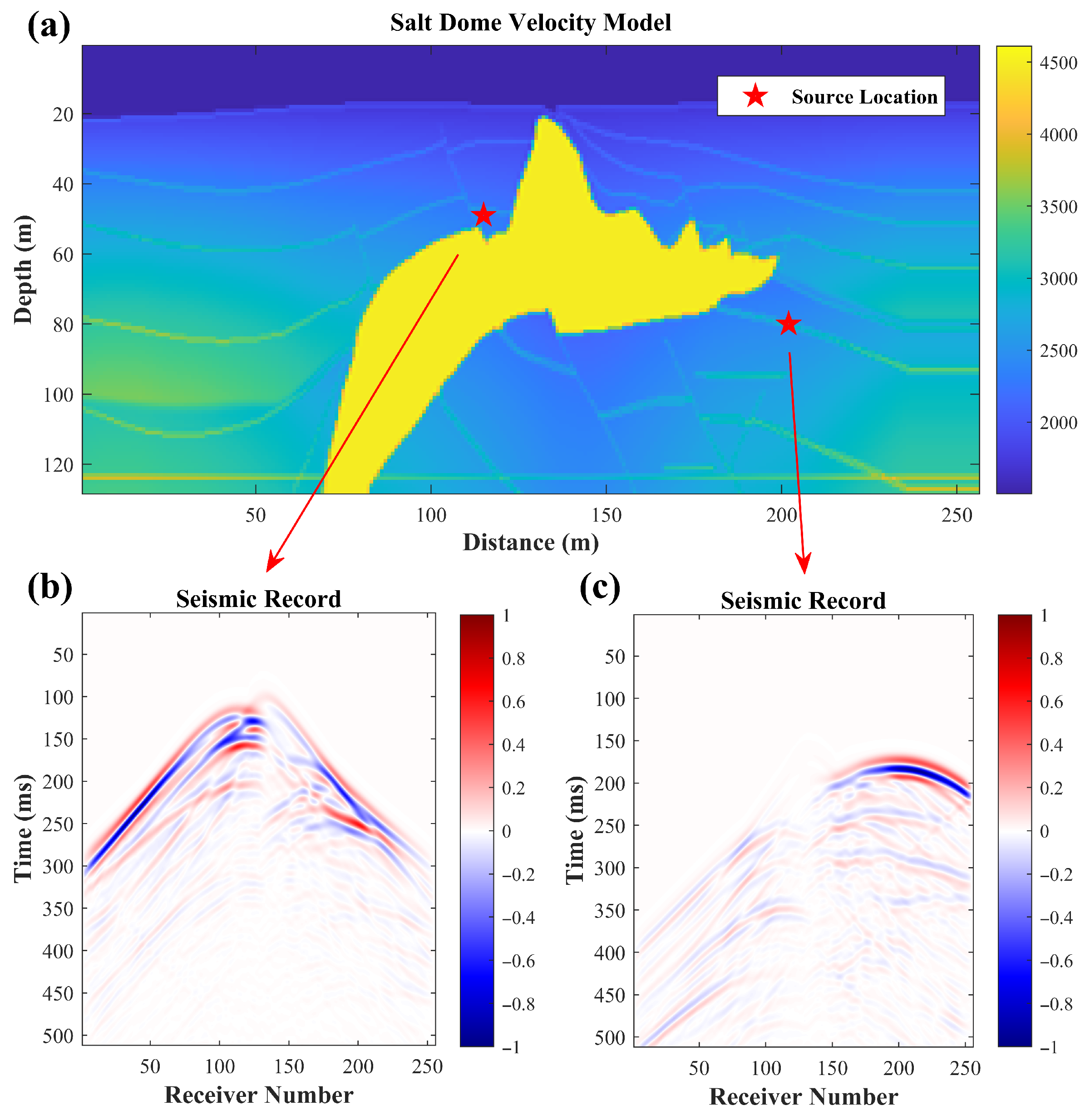
The salt dome velocity model used in this experiment measures 256 m in the east-west direction and 128 m in depth, with a known subsurface velocity ranging from 1500 m/s to 4000 m/s. In this forward simulation, 256 receivers are positioned on the surface, and the seismic signals received by each receiver are simulated using the finite-difference method for the acoustic wave equation. A total of 7500 source points are randomly selected within the salt dome model to generate seismic signals, forming the dataset. Of these, 6000 are used for self-supervised training, 500 for supervised training, 500 for validation, and 500 for testing. The velocity model and seismic records for different sources are shown in Figure 5.
Figure 5.
Salt Dome Model and Seismic Records Corresponding to Different Sources: (a) Velocity distribution and two source locations. (b) Seismic record from Source 1. (c) Seismic record from Source 2.
During training, we standardized hyperparameter settings for both the self-supervised and supervised training phases to maintain consistent experimental conditions. Specifically, the batch size was set to 32, mean squared error (MSE) was used as the loss function, and the initial learning rate was set to 0.0001. In the self-supervised training phase, the model was trained for 500 epochs to thoroughly capture features from the seismic data. In the supervised training phase, we applied the same hyperparameters across all four networks and implemented a learning rate decay strategy, reducing the learning rate by a factor of 10 every 100 epochs, for a total of 300 epochs, to optimize localization performance.
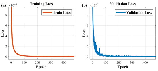
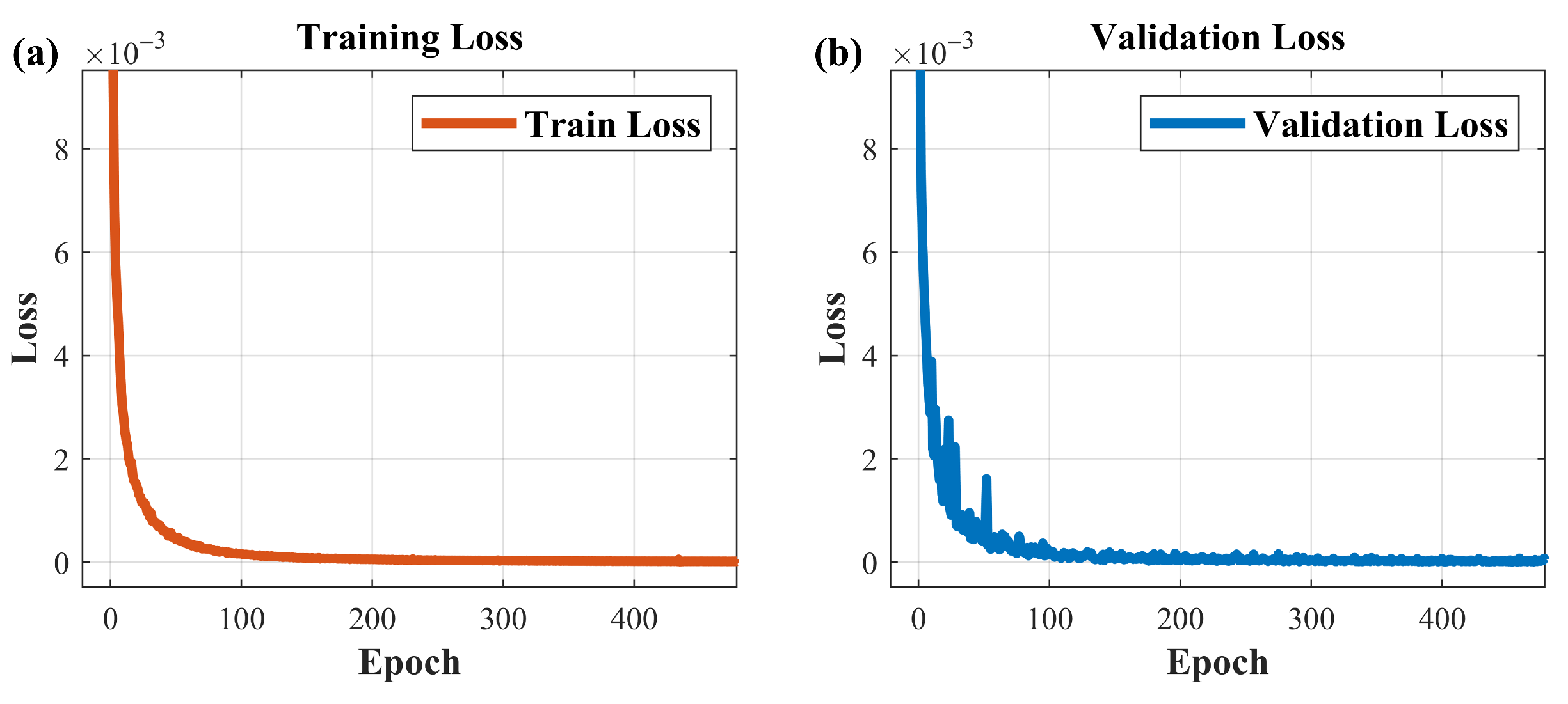
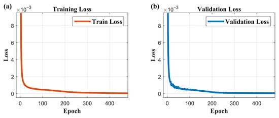
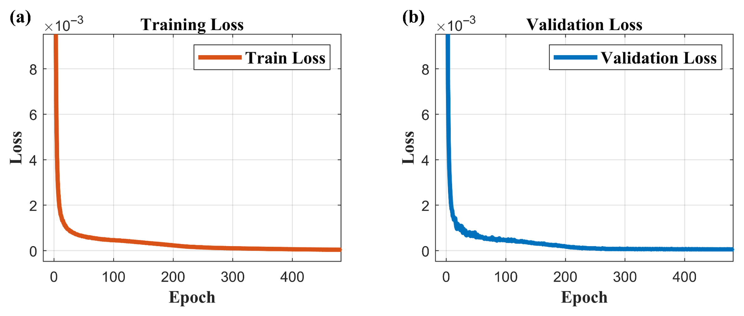
In the self-supervised learning phase, the RCAE was trained to reconstruct seismic data, as shown in Figure 6. The loss function value gradually decreased over the training epochs, showing a clear convergence trend. After 500 epochs, the loss value stabilized, indicating successful network training.
Figure 6.
Training Loss Curves (a) and Validation Loss Curves (b) in Self-supervised Learning Based on the 2D Salt Dome Model.
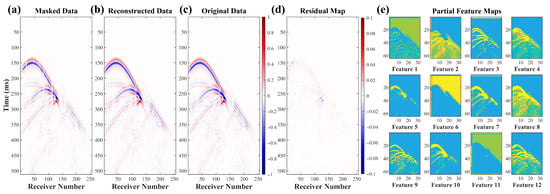
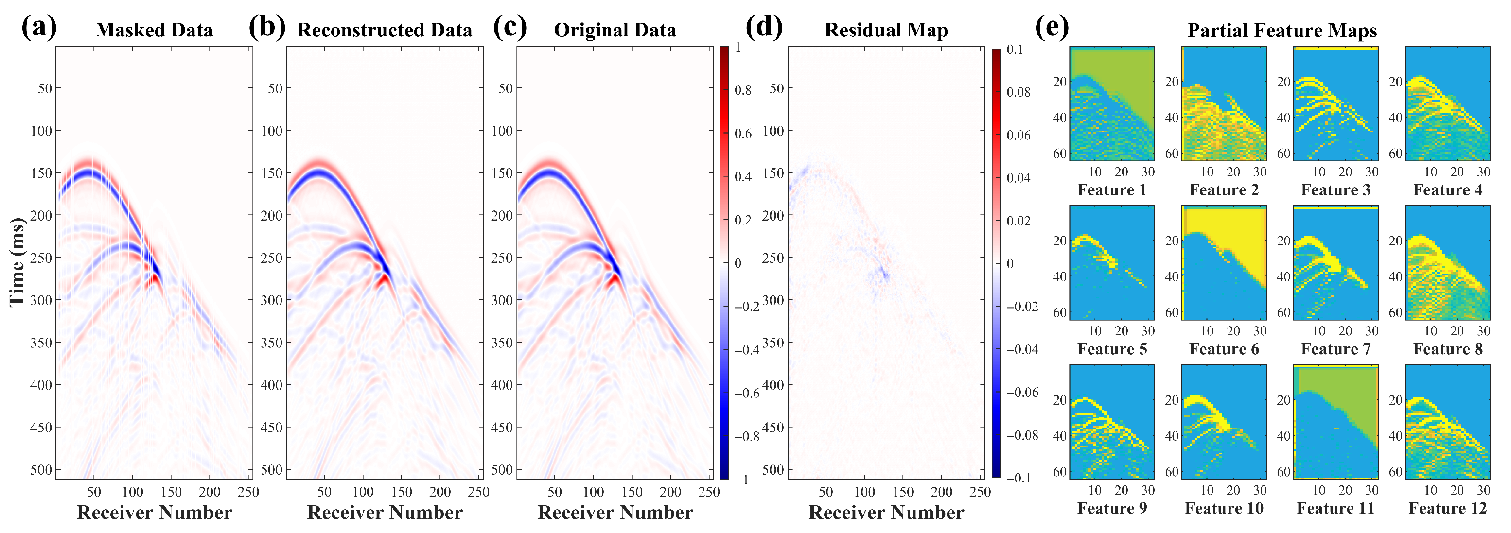
We then tested the trained model on the test set for reconstruction. As shown in Figure 7, a selected seismic record demonstrates that the RCAE successfully restored a nearly continuous seismic record from a 20% masked, discontinuous record; moreover, the residual map shows only minor differences between the two, demonstrating the effectiveness of the self-supervised pre-training. Additionally, the average reconstruction error across 500 test samples was only , confirming the high consistency between the reconstructed and original records.
Figure 7.
Self-supervised seismic data processing results on a Test Sample: (a) Masked input: Partially obscured seismic traces used as network input. (b) Reconstructed output: Network prediction with restored waveform features. (c) Original data: Ground truth seismic record for comparison. (d) Residual: Difference (original-reconstructed) highlighting reconstruction errors. (e) Encoder features: Extracted partial feature maps from seismic records.
The partial feature maps in Figure 7 show that the encoder effectively captured key seismic features, such as first arrival waves and hyperbolic reflection patterns. These rich, multidimensional features are essential for subsequent seismic event localization. The features extracted by the pre-trained model will significantly enhance performance in small-sample supervised learning, making it more effective in handling limited data. Ultimately, we selected the model obtained after 500 epochs as the pre-trained model for the subsequent small-sample microseismic localization task.
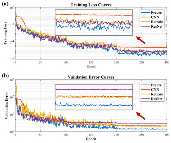
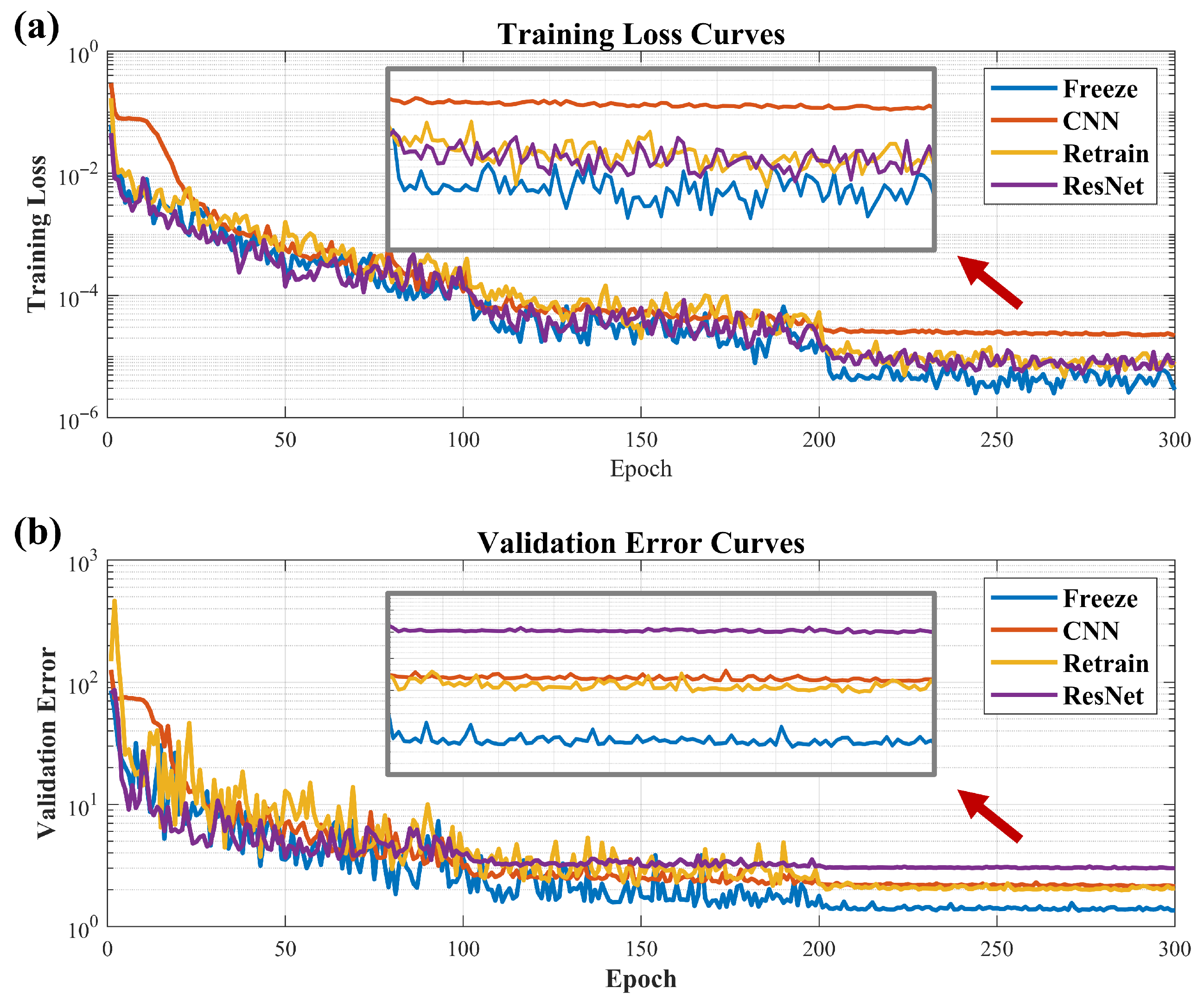
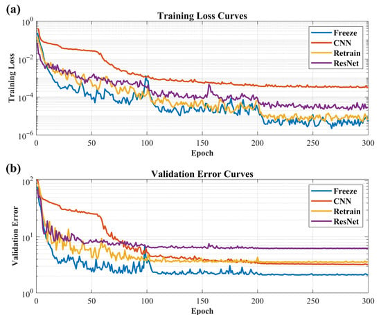
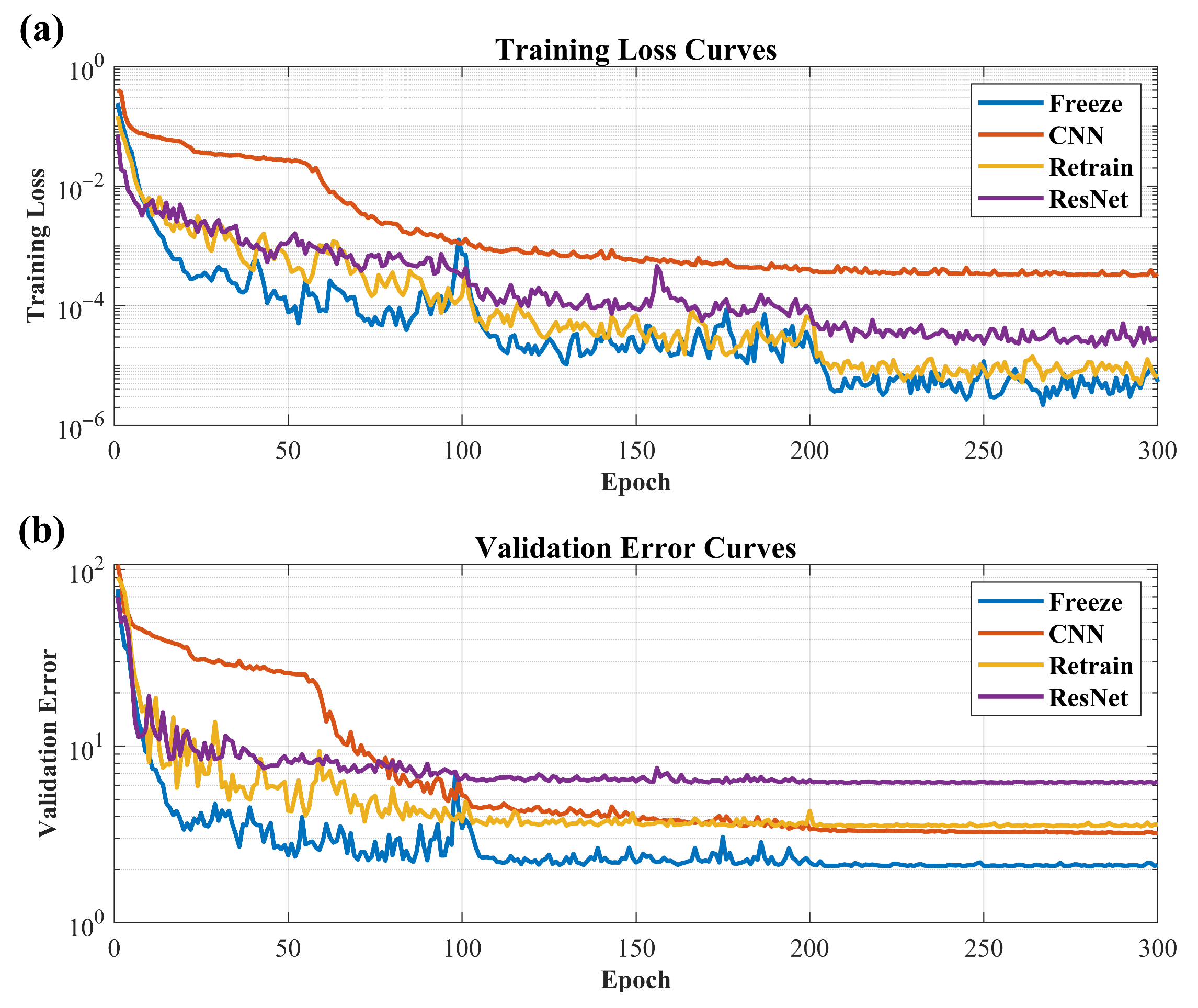
In the supervised learning phase, we trained using only 500 labeled seismic records. As shown in Figure 8, the training loss curves and average localization error curves on the validation set reflect each method’s performance. Analysis shows that the Freeze method, which uses a frozen pre-trained encoder, consistently achieved the lowest error on both the training and validation sets, indicating stronger generalization to unseen data. The Retrain method follows in performance, while the CNN model, though performing poorly on the training set, showed better results on the validation set. In contrast, the ResNet method achieved lower loss on the training set but had higher error on the validation set, likely due to overfitting from its deeper network structure on the small-sample dataset.
Figure 8.
Training performance comparison on the salt dome model: (a) Training loss curve. (b) Validation error curve. The Freeze strategy (blue) achieves the lowest final error, demonstrating optimal convergence.
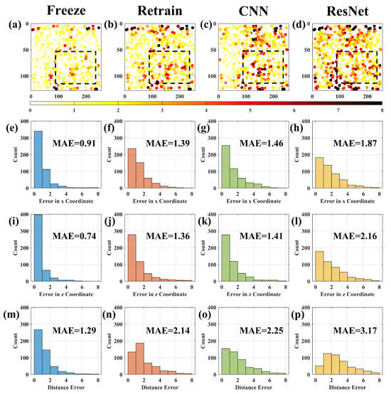
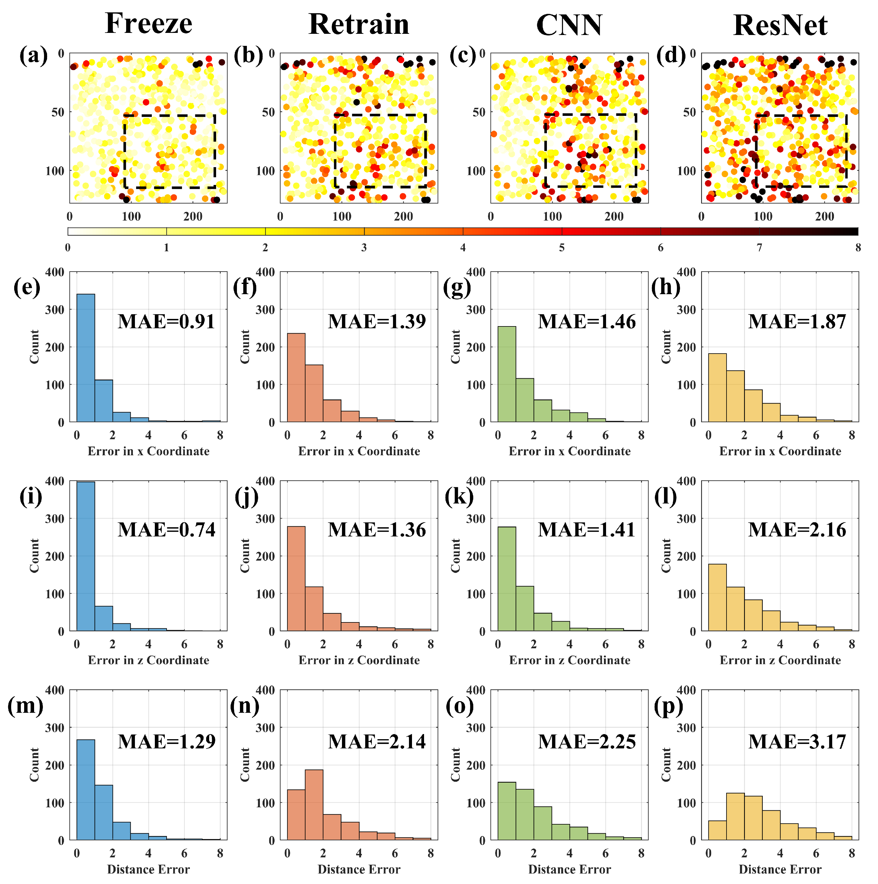
After training, we applied the four methods to localize sources in the test set, with results shown in Figure 9. Figure 9a–d display the localization error distributions for each method, where dots represent the actual source locations of the 500 test samples, and the color intensity reflects the magnitude of localization error. Observing the color distribution within the black frame, we see that the Freeze method has the lightest color, indicating a clear advantage in localization accuracy over the other three methods. Figure 9e–p provide error statistics that further support this observation. The mean absolute error (MAE) shows that the Freeze method’s error distribution is closest to zero for the x-axis, z-axis, and total distance errors (defined as the Euclidean distance between the true source coordinates and the predicted coordinates). The calculated average distance error is only 1.29 m, demonstrating the highest accuracy. In comparison, the Retrain and CNN methods have average errors of 2.14 m and 2.25 m, respectively. The ResNet method, with an average error of 3.17 m, shows the poorest performance, likely due to overfitting caused by a mismatch between the model’s complexity and the small sample size, resulting in suboptimal localization. Overall, these results demonstrate that our semi-supervised learning method offers significant advantages over traditional supervised methods for small-sample data, effectively enhancing model generalization and localization accuracy.
Figure 9.
Localization Error Distributions and Statistical Charts for Four Methods: (a–d) The localization error distributions of 500 test events. Each dot represents a true source location, and the color indicates the absolute distance error—the lighter the color, the smaller the error. The Freeze strategy exhibits the lowest errors, especially in the highlighted region. (e–p) Histograms of errors in the x and z directions, as well as total distance errors. The Freeze model achieves the lowest mean absolute error (MAE) across all metrics.
3.2. 3D Velocity Model
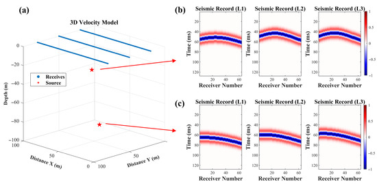
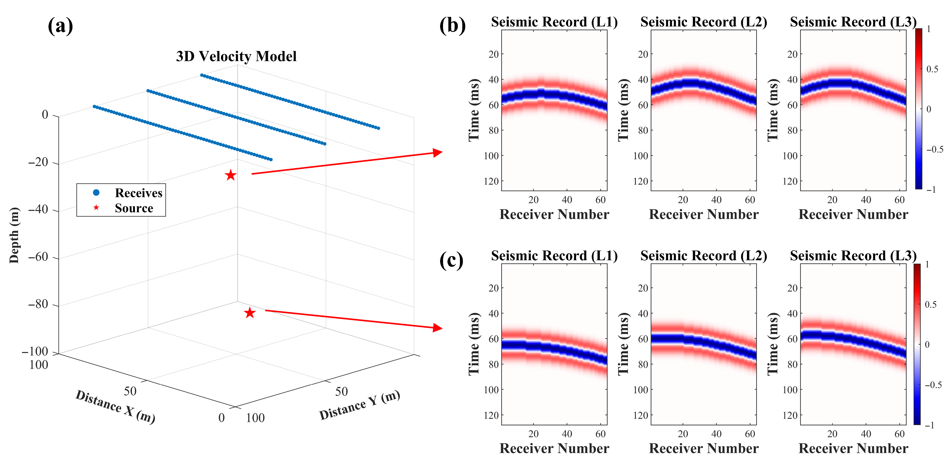
In addition to the 2D salt dome model, we also tested the proposed semi-supervised localization method on a 3D velocity model. This model spans 100 m in the east–west and north–south directions and 100 m in depth, with a subsurface velocity set to 1500 m/s. Three receiver lines were deployed on the surface, each with 64 receivers, and the recorded seismic signals served as three-channel inputs to the network. A total of 7600 source points were randomly selected within the model for forward modeling to produce seismic signals. Of these, 6000 were used for self-supervised training, 300 for supervised training, 300 for validation, and 1000 for testing. The 3D velocity model and seismic records for different sources are shown in Figure 10.
Figure 10.
3D Velocity Model and Seismic Records Corresponding to Different Sources: (a) 3D velocity structure with two seismic sources (red stars) and receiver array (blue dots). (b,c) Shot gathers along three receiver lines (L1, L2, L3) for two sources.
The training approach for the 3D velocity model mirrors that of the salt dome model, beginning with self-supervised training and followed by supervised learning with a small number of labeled seismic records. Due to the different data dimensions, we adjusted the output dimension of the final fully connected layer in the localization network to 3. All other network structures and hyperparameter settings were kept the same as those used for the salt dome model.
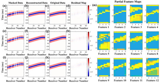
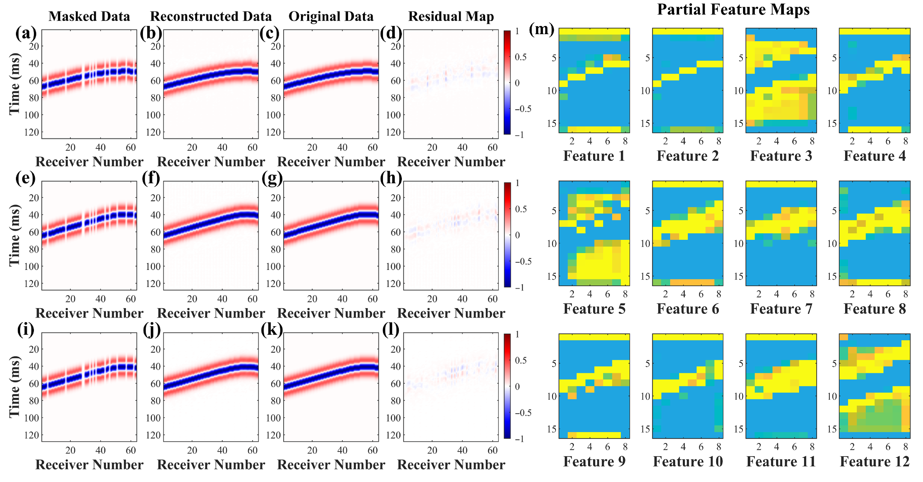
As shown in Figure 11, the loss and validation curves in the self-supervised learning process converge after 500 training epochs. Figure 12 displays the reconstructed seismic records, reconstruction residual map and extracted partial feature maps from the test set, with an average reconstruction error of . This low error confirms that the encoder has been successfully trained and can effectively extract features from seismic records.
Figure 11.
Training Loss Curves (a) and Validation Loss Curves (b) in Self-supervised Learning Based on the 3D Velocity Model.
Figure 12.
Reconstructed Seismic Records and Encoder Feature Maps from RCAE. (a–l) Reconstruction results for one seismic event recorded on three receiver lines (L1–L3). Each row presents the masked input (a,e,i), the reconstructed output from RCAE (b,f,j), the original complete data (c,g,k), and the corresponding residual maps (d,h,l) for each of the three receiver lines. (m) Partial feature maps extracted by the encoder, illustrating its ability to effectively represent seismic signal characteristics.
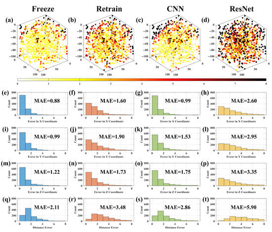
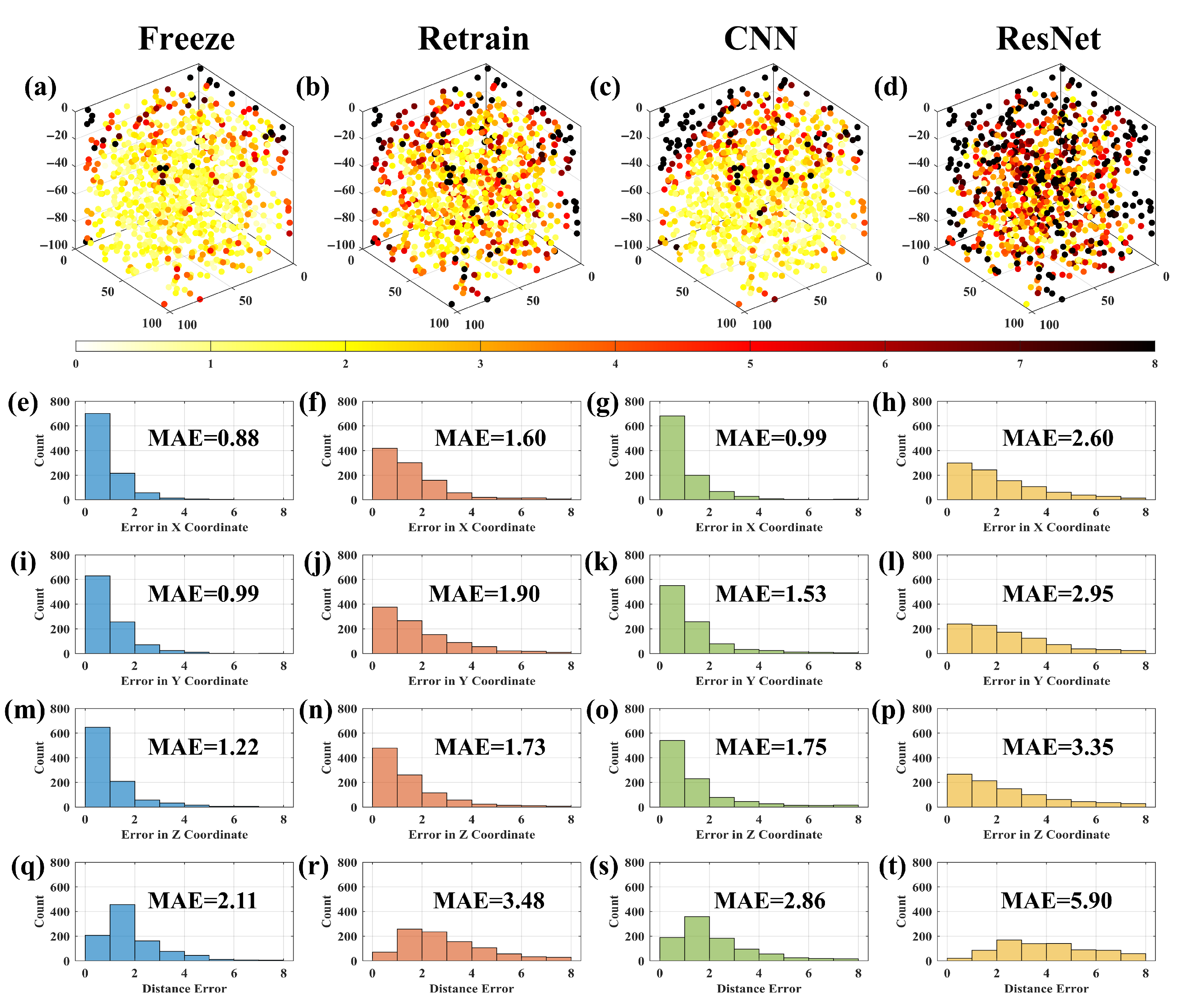
Figure 13 shows the loss and validation error curves during supervised learning, with the Freeze method achieving the lowest error rate. Figure 14 provides detailed localization results and error statistics for 1000 test samples. The error distribution maps in Figure 14a–d show that the Freeze method has the smallest localization error at shallow surface locations, indicated by a visibly lighter color compared to other methods. Figure 14e–t display statistical charts for the x-axis, y-axis, z-axis, and total distance errors. Together with the calculated average error values, these charts emphasize the Freeze method’s advantage in localization accuracy. In comparison with the baseline CNN model, we find that while the Retrain and Freeze methods use the same network structure, the Retrain method’s localization performance falls short of the CNN model. In contrast, the Freeze method, by leveraging the encoder parameters from self-supervised training, achieves higher accuracy than the CNN model. Although the ResNet model shows lower loss values during training, its performance on the validation and test sets did not meet expectations, indicating that deep network structures may not be ideal with limited training samples. This underscores the importance of selecting an appropriate network depth and structure in small-sample training environments. Overall, for the 3D velocity model, the semi-supervised learning method offers superior performance compared to traditional supervised learning methods.
Figure 13.
Training performance comparison on 3D velocity model: (a) Training loss curve. (b) Validation error curve. As shown, the Freeze strategy (blue line) achieves the lowest training loss and validation error.
Figure 14.
Performance Comparison of Four Models on the 3D Source Localization Task. Subfigures (a–d) show the 3D localization error distributions of 1000 test events. Each dot represents a true source location, and the color indicates the absolute distance error—the lighter the color, the smaller the error. Subfigures (e–t) present histograms of errors in the x, y, and z directions, as well as the total distance error. The Freeze model achieves the lowest mean absolute error (MAE) across all metrics, demonstrating superior accuracy.
4. Discussion
4.1. Impact of Masking Ratio
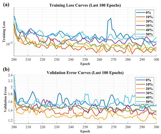
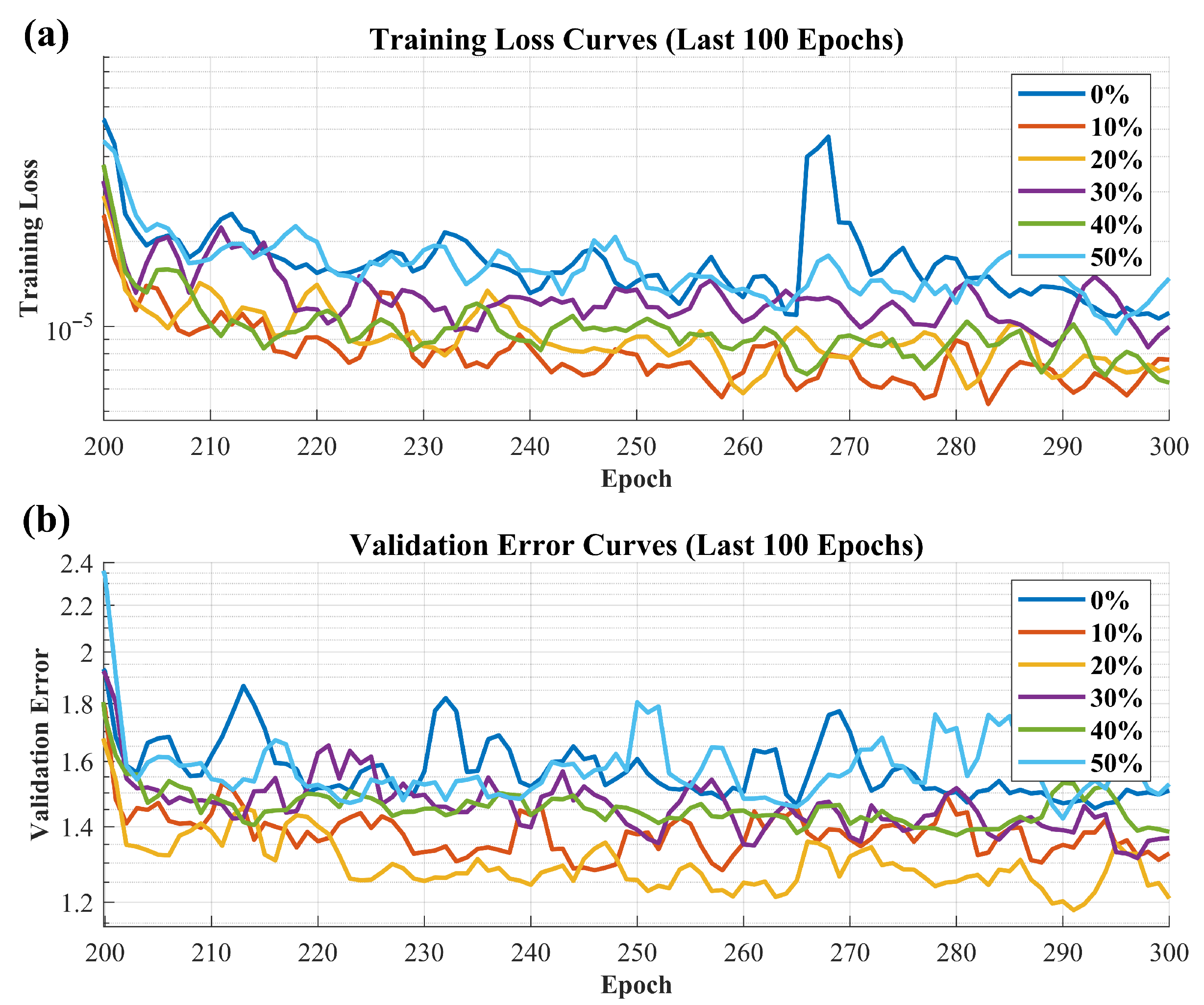
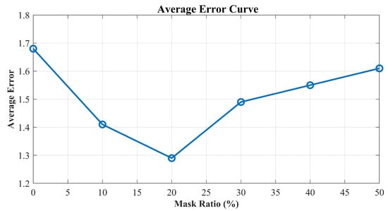
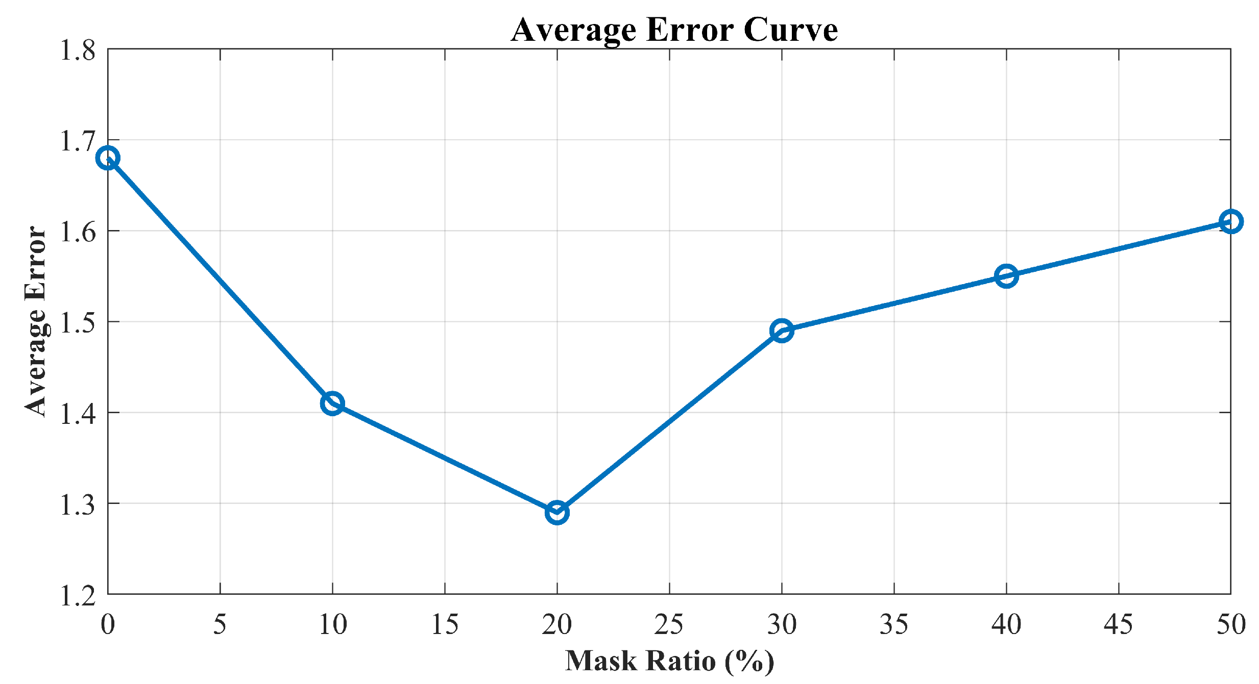
In this section, we use the salt dome model to examine how different masking ratios in self-supervised learning affect seismic data feature extraction and localization accuracy. Keeping other parameters constant, we trained the RCAE on seismic records with masking ratios ranging from 10% to 50%. After self-supervised training, the encoder parameters were used in supervised learning to train the localization network. During supervised learning, we recorded the training loss curve and average localization error curve on the validation set, as shown in Figure 15, where a 20% masking ratio yielded the lowest average error. Next, we tested the localization performance on 500 test samples and calculated the corresponding average localization error. These results are summarized in Table 1 and visualized in Figure 16.
Figure 15.
Training Loss Curve (a) and Validation Set Average Error Curve (b) in Supervised Learning with Different Masking Ratios.
Table 1.
Average Localization Error at Different Masking Ratios.
Figure 16.
Line Chart of Average Localization Error at Different Masking Ratios. The lowest error occurs at a 20% masking ratio.
The experimental results indicate that as the masking ratio increases, localization accuracy improves, reaching its lowest error at a 20% masking ratio. This may be because a low masking ratio leaves most information accessible, so the model does not effectively learn to extract essential features. A higher masking ratio encourages the network to learn deeper, more robust feature representations. However, when the masking ratio exceeds a certain threshold, localization accuracy decreases, suggesting that too much masking leads to information loss, which hinders the network’s ability to learn effective features. Thus, choosing an appropriate masking ratio can effectively enhance final localization accuracy.
4.2. Impact of Labeled Sample Quantity
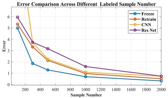
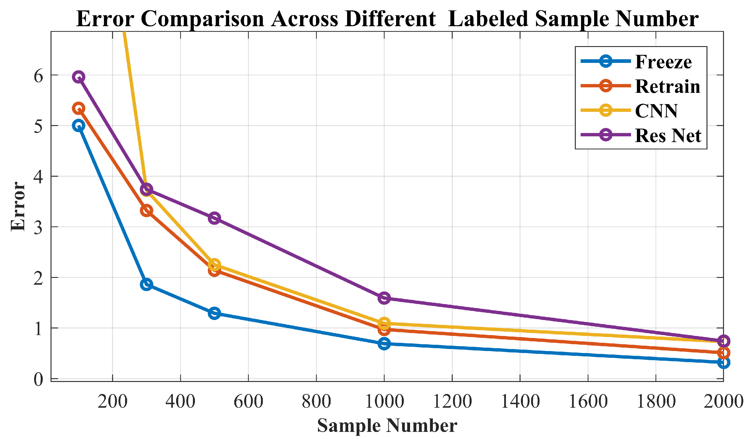
In this section, we continue using the salt dome model to assess how the number of labeled samples affects localization accuracy. The experimental parameters remained unchanged, and we trained the network using labeled sample sizes from 100 to 2000 to compare the localization performance of the four methods at different sample quantities. After training, we evaluated each method’s localization performance on 500 test samples and recorded the average localization error, as shown in Table 2. The line chart in Figure 17 visually illustrates these results.
Table 2.
Average Localization Error of Four Methods with Different Numbers of Labeled Samples.
Figure 17.
Line Chart of Average Localization Error of Four Methods with Different Numbers of Labeled Samples. Freeze consistently yields the lowest error, with clear advantages under limited labeled data.
Analysis shows that when the sample size is very small (only 100 samples), the CNN method’s localization performance is most affected, with the highest error. As the number of labeled samples increases, all methods show significant improvements in localization accuracy. However, the Freeze method consistently achieves the lowest error across all sample sizes, with its advantage particularly evident when sample sizes are below 1000. This is due to the self-supervised training of the encoder in the Freeze method, which enables it to effectively extract key features for accurate localization even with limited labeled data. As the sample size exceeds 1000, all methods benefit from the increased data, and the error gap narrows, but the Freeze method still maintains the lowest error level. This suggests that the proposed semi-supervised learning method not only excels in low-sample scenarios but also significantly enhances localization accuracy when data are more abundant.
Overall, these results demonstrate the effectiveness of semi-supervised learning in label-scarce environments and its robustness when larger amounts of data are available.
5. Conclusions
Microseismic localization is a critical technique for ensuring operational safety and optimizing production efficiency in engineering applications such as hydraulic fracturing and mineral extraction. Its accuracy directly affects the safety and overall effectiveness of engineering operations and thus plays an indispensable role in practical applications. However, most existing deep learning-based microseismic localization methods rely on supervised learning paradigms that require large-scale labeled datasets. In real production scenarios, obtaining accurate source labels is costly, labor-intensive, and often impractical at scale. To address this challenge, this study proposes a semi-supervised microseismic localization method based on a residual convolutional autoencoder (RCAE). The proposed approach first performs masked reconstruction pre-training on unlabeled seismic data, which significantly enhances the encoder’s ability to extract essential features from seismic records. Subsequently, the localization network is fine-tuned using a limited number of labeled samples. Experimental results demonstrate that the proposed method effectively improves microseismic localization accuracy under label-scarce conditions. Experimental results demonstrate that the proposed method outperforms traditional fully supervised learning approaches on both 2D salt dome and 3D velocity models. Additionally, the study indicates that selecting an appropriate masking ratio can further boost localization precision. Tests across various data volumes confirm the method’s effectiveness in data-scarce scenarios, while also yielding significant localization improvements when more samples are available. Overall, the semi-supervised learning strategy introduced herein reduces dependence on extensive labeled datasets, providing a cost-effective solution for advancing microseismic localization techniques.
Author Contributions
Conceptualization, Z.W. and X.G.; methodology, Z.W.; software, Z.W.; validation, Z.W.; formal analysis, Z.W.; investigation, Z.W.; writing—original draft preparation, Z.W.; writing—review and editing, Z.W., Q.C., Z.C. and X.L.; visualization, Z.W.; supervision, X.G. and Z.X.; project administration, X.G.; funding acquisition, X.G. All authors have read and agreed to the published version of the manuscript.
Funding
This work was supported in part by the Deep Earth Probe and Mineral Resources Exploration-National Science and Technology Major Project under Grant 2024ZD1004101, in part by the National Natural Science Foundation of China under Grant 42274164 and Grant 42074151.
Data Availability Statement
The data are available by contacting Zhe Wang.
Conflicts of Interest
The authors declare no conflicts of interest.
References
- Li, N.; Fang, L.; Sun, W.; Zhang, X.; Chen, D. Evaluation of borehole hydraulic fracturing in coal seam using the microseismic monitoring method. Rock Mech. Rock Eng. 2021, 54, 607–625. [Google Scholar] [CrossRef] [Scilit]
- Li, N.; Wang, E.; Ge, M. Microseismic monitoring technique and its applications at coal mines: Present status and future prospects. J. China Coal Soc. 2017, 42, 83–96. [Google Scholar]
- Xiao, Y.X.; Feng, X.T.; Hudson, J.A.; Chen, B.R.; Feng, G.L.; Liu, J.P. ISRM suggested method for in situ microseismic monitoring of the fracturing process in rock masses. Rock Mech. Rock Eng. 2016, 49, 343–369. [Google Scholar] [CrossRef] [Scilit]
- Warpinski, N. Microseismic monitoring: Inside and out. J. Pet. Technol. 2009, 61, 80–85. [Google Scholar] [CrossRef] [Scilit]
- Geiger, L. Probability method for the determination of earthquake epicentres from the arrival time only. Bull. St. Louis Univ. 1912, 8, 60. [Google Scholar]
- Waldhauser, F.; Ellsworth, W.L. A double-difference earthquake location algorithm: Method and application to the northern Hayward fault, California. Bull. Seismol. Soc. Am. 2000, 90, 1353–1368. [Google Scholar] [CrossRef] [Scilit]
- Powell, M.J. An efficient method for finding the minimum of a function of several variables without calculating derivatives. Comput. J. 1964, 7, 155–162. [Google Scholar] [CrossRef] [Scilit]
- Liao, Y.C.; Kao, H.; Rosenberger, A.; Hsu, S.K.; Huang, B.S. Delineating complex spatiotemporal distribution of earthquake aftershocks: An improved source-scanning algorithm. Geophys. J. Int. 2012, 189, 1753–1770. [Google Scholar] [CrossRef] [Scilit]
- Lu, R.; Lazaratos, S.; Wang, K.; Cha, Y.; Chikichev, I.; Prosser, R. High-resolution elastic FWI for reservoir characterization. In Proceedings of the 75th EAGE Conference & Exhibition Incorporating SPE EUROPEC 2013, London, UK, 10–13 June 2013; European Association of Geoscientists & Engineers: Bunnik, The Netherlands; p. 348. [Google Scholar]
- Zurada, J.M.; Marks, I.; Robinson, C.J. Computational Intelligence Imitating Life; Technical Report; Institute of Electrical and Electronics Engineers, Inc.: New York, NY, USA, 1994. [Google Scholar]
- Wang, H.; Alkhalifah, T. Microseismic imaging using a source function independent full waveform inversion method. Geophys. J. Int. 2018, 214, 46–57. [Google Scholar] [CrossRef] [Scilit]
- Song, C.; Alkhalifah, T.; Wu, Z. Microseismic event estimation and velocity analysis based on a source-focusing function. Geophysics 2019, 84, KS85–KS94. [Google Scholar] [CrossRef] [Scilit]
- Kao, H.; Shan, S.J.; Dragert, H.; Rogers, G.; Cassidy, J.F.; Ramachandran, K. A wide depth distribution of seismic tremors along the northern Cascadia margin. Nature 2005, 436, 841–844. [Google Scholar] [CrossRef] [Scilit] [PubMed]
- Kao, H.; Shan, S.J. The source-scanning algorithm: Mapping the distribution of seismic sources in time and space. Geophys. J. Int. 2004, 157, 589–594. [Google Scholar] [CrossRef] [Scilit]
- Nakata, N.; Beroza, G.C. Reverse time migration for microseismic sources using the geometric mean as an imaging condition. Geophysics 2016, 81, KS51–KS60. [Google Scholar] [CrossRef] [Scilit]
- Wu, S.; Wang, Y.; Zheng, Y.; Chang, X. Microseismic source locations with deconvolution migration. Geophys. J. Int. 2018, 212, 2088–2115. [Google Scholar] [CrossRef] [Scilit]
- Larmat, C.; Montagner, J.P.; Fink, M.; Capdeville, Y.; Tourin, A.; Clévédé, E. Time-reversal imaging of seismic sources and application to the great Sumatra earthquake. Geophys. Res. Lett. 2006, 33, L19312. [Google Scholar] [CrossRef] [Scilit]
- Perol, T.; Gharbi, M.; Denolle, M. Convolutional neural network for earthquake detection and location. Sci. Adv. 2018, 4, e1700578. [Google Scholar] [CrossRef] [Scilit]
- Bai, T.; Tahmasebi, P. Attention-based LSTM-FCN for earthquake detection and location. Geophys. J. Int. 2022, 228, 1568–1576. [Google Scholar] [CrossRef] [Scilit]
- Kriegerowski, M.; Petersen, G.M.; Vasyura-Bathke, H.; Ohrnberger, M. A deep convolutional neural network for localization of clustered earthquakes based on multistation full waveforms. Seismol. Res. Lett. 2019, 90, 510–516. [Google Scholar] [CrossRef] [Scilit]
- van den Ende, M.P.; Ampuero, J.P. Automated seismic source characterization using deep graph neural networks. Geophys. Res. Lett. 2020, 47, e2020GL088690. [Google Scholar] [CrossRef] [Scilit]
- Wamriew, D.; Charara, M.; Pissarenko, D. Joint event location and velocity model update in real-time for downhole microseismic monitoring: A deep learning approach. Comput. Geosci. 2022, 158, 104965. [Google Scholar] [CrossRef] [Scilit]
- Feng, Q.; Han, L.; Pan, B.; Zhao, B. Microseismic source location using deep reinforcement learning. IEEE Trans. Geosci. Remote Sens. 2022, 60, 4510209. [Google Scholar] [CrossRef] [Scilit]
- Zhang, X.; Zhang, J.; Yuan, C.; Liu, S.; Chen, Z.; Li, W. Locating induced earthquakes with a network of seismic stations in Oklahoma via a deep learning method. Sci. Rep. 2020, 10, 1941. [Google Scholar] [CrossRef] [Scilit] [PubMed]
- Wang, H.; Alkhalifah, T.; bin Waheed, U.; Birnie, C. Data-driven microseismic event localization: An application to the Oklahoma Arkoma basin hydraulic fracturing data. IEEE Trans. Geosci. Remote Sens. 2021, 60, 4506212. [Google Scholar] [CrossRef] [Scilit]
- Vinard, N.; Drijkoningen, G.; Verschuur, D. Localizing microseismic events on field data using a U-Net-based convolutional neural network trained on synthetic data. Geophysics 2022, 87, KS33–KS43. [Google Scholar] [CrossRef] [Scilit]
- Sheng, H.; Wu, X.; Si, X.; Li, J.; Zhang, S.; Duan, X. Seismic Foundation Model (SFM): A new generation deep learning model in geophysics. arXiv 2023, arXiv:2309.02791. [Google Scholar] [CrossRef] [Scilit]
- Saad, O.M.; Oboue, Y.A.S.I.; Bai, M.; Samy, L.; Yang, L.; Chen, Y. Self-attention deep image prior network for unsupervised 3-D seismic data enhancement. IEEE Trans. Geosci. Remote Sens. 2021, 60, 5907014. [Google Scholar] [CrossRef] [Scilit]
- Wang, H.; Lin, J.; Li, Y.; Dong, X.; Tong, X.; Lu, S. Self-Supervised Pre-Training Transformer for Seismic Data Denoising. IEEE Trans. Geosci. Remote Sens. 2024, 62, 5907525. [Google Scholar]
- Xu, Z.; Luo, Y.; Wu, B.; Meng, D.; Chen, Y. Deep nonlocal regularizer: A self-supervised learning method for 3d seismic denoising. IEEE Trans. Geosci. Remote Sens. 2023, 61, 5921517. [Google Scholar] [CrossRef] [Scilit]
- Saad, O.M.; Chen, Y. A fully unsupervised and highly generalized deep learning approach for random noise suppression. Geophys. Prospect. 2021, 69, 709–726. [Google Scholar] [CrossRef] [Scilit]
- Fang, W.; Fu, L.; Wu, M.; Yue, J.; Li, H. Irregularly sampled seismic data interpolation with self-supervised learning. Geophysics 2023, 88, V175–V185. [Google Scholar] [CrossRef] [Scilit]
- Yuan, P.; Wang, S.; Hu, W.; Nadukandi, P.; Botero, G.O.; Wu, X.; Van Nguyen, H.; Chen, J. Self-supervised learning for efficient antialiasing seismic data interpolation. IEEE Trans. Geosci. Remote Sens. 2022, 60, 5913819. [Google Scholar] [CrossRef] [Scilit]
- Song, A.; Wang, C.; Zhang, C.; Zhang, J.; Xiong, D.; Wei, X. Regeneration-constrained self-supervised seismic data interpolation. IEEE Trans. Geosci. Remote Sens. 2023, 61, 5901610. [Google Scholar] [CrossRef] [Scilit]
- Li, Y.; Alkhalifah, T.; Huang, J.; Li, Z. Self-supervised pre-training vision transformer with masked autoencoders for building subsurface model. IEEE Trans. Geosci. Remote Sens. 2023, 61, 4506610. [Google Scholar]
- Li, Y.; Cao, W.; Lu, W.; Huang, X.; Ding, J.; Song, C. Reconstruct 3D seismic data with randomly missing traces via fast self-supervised deep learning. IEEE Trans. Geosci. Remote Sens. 2024, 62, 5915814. [Google Scholar]
- Feng, Q.; Han, L.; Zhao, B. Localizing microseismic events using semi-supervised generative adversarial networks. IEEE Trans. Geosci. Remote Sens. 2022, 60, 5923908. [Google Scholar] [CrossRef] [Scilit]
- Si, X.; Wu, X.; Sheng, H.; Zhu, J.; Li, Z. SeisCLIP: A seismology foundation model pre-trained by multi-modal data for multi-purpose seismic feature extraction. IEEE Trans. Geosci. Remote Sens. 2024, 62, 5903713. [Google Scholar]
- He, K.; Zhang, X.; Ren, S.; Sun, J. Deep residual learning for image recognition. In Proceedings of the IEEE Conference on Computer Vision and Pattern Recognition, Las Vegas, NV, USA, 27–30 June 2016; pp. 770–778. [Google Scholar]
- Zhang, Y. A Better Autoencoder for Image: Convolutional Autoencoder. 2018. Available online: https://users.cecs.anu.edu.au/~Tom.Gedeon/conf/ABCs2018/paper/ABCs2018_paper_58.pdf (accessed on 23 March 2017).
- Masci, J.; Meier, U.; Cireşan, D.; Schmidhuber, J. Stacked convolutional auto-encoders for hierarchical feature extraction. In Proceedings of the Artificial Neural Networks and Machine Learning–ICANN 2011: 21st International Conference on Artificial Neural Networks, Espoo, Finland, 14–17 June 2011; Proceedings, Part I 21. Springer: Berlin/Heidelberg, Germany, 2011; pp. 52–59. [Google Scholar]
- Kong, Q.; Chiang, A.; Aguiar, A.C.; Fernández-Godino, M.G.; Myers, S.C.; Lucas, D.D. Deep convolutional autoencoders as generic feature extractors in seismological applications. Artif. Intell. Geosci. 2021, 2, 96–106. [Google Scholar] [CrossRef] [Scilit]
- Mousavi, S.M.; Zhu, W.; Ellsworth, W.; Beroza, G. Unsupervised clustering of seismic signals using deep convolutional autoencoders. IEEE Geosci. Remote Sens. Lett. 2019, 16, 1693–1697. [Google Scholar] [CrossRef] [Scilit]
- Helal, E.B.; Saad, O.M.; Hafez, A.G.; Chen, Y.; Dousoky, G.M. Seismic data compression using deep learning. IEEE Access 2021, 9, 58161–58169. [Google Scholar] [CrossRef] [Scilit]
- Vincent, P.; Larochelle, H.; Bengio, Y.; Manzagol, P.A. Extracting and composing robust features with denoising autoencoders. In Proceedings of the 25th International Conference on Machine Learning, Helsinki, Finland, 5–9 July 2008; pp. 1096–1103. [Google Scholar]
- Bergamasco, L.; Saha, S.; Bovolo, F.; Bruzzone, L. Unsupervised change-detection based on convolutional-autoencoder feature extraction. In Proceedings of the Image and Signal Processing for Remote Sensing XXV, Strasbourg, France, 9–11 September 2019; SPIE: Bellingham, WA, USA, 2019; Volume 11155, pp. 325–332. [Google Scholar]
- He, F.; Liu, T.; Tao, D. Why resnet works? residuals generalize. IEEE Trans. Neural Netw. Learn. Syst. 2020, 31, 5349–5362. [Google Scholar] [CrossRef] [Scilit]
- He, K.; Zhang, X.; Ren, S.; Sun, J. Identity mappings in deep residual networks. In Proceedings of the Computer Vision–ECCV 2016: 14th European Conference, Amsterdam, The Netherlands, 11–14 October 2016; Proceedings, Part IV 14. Springer: Berlin/Heidelberg, Germany, 2016; pp. 630–645. [Google Scholar]

Disclaimer/Publisher’s Note: The statements, opinions and data contained in all publications are solely those of the individual author(s) and contributor(s) and not of MDPI and/or the editor(s). MDPI and/or the editor(s) disclaim responsibility for any injury to people or property resulting from any ideas, methods, instructions or products referred to in the content. |
© 2026 by the authors. Licensee MDPI, Basel, Switzerland. This article is an open access article distributed under the terms and conditions of the Creative Commons Attribution (CC BY) license.