Calibration of Snow Particle Contact Parameters for Simulation Analysis of Membrane Structure Snow Removal Robot

Abstract

To enhance the accuracy of discrete element method (DEM) simulation for the snow removal process performed by autonomous robots on membrane structures, this study calibrated the key contact parameters of snow particles used in the simulation. Through literature research, the intrinsic parameters and contact parameter ranges for snow particles and membrane structures were determined. A discrete element model of snow particles was established, and the Hertz–Mindlin with Johnson–Kendall–Robert contact model was selected to simulate the formation process of the repose angle. Using the actual repose angle of snow particles as the target, four significant factors were identified through the P-B experiment, and other factors were set at the intermediate level. Through the steepest slope climbing experiment and response surface design, second-order response equations of the four significant factors were obtained. The optimal parameter combination was calculated as follows: the surface energy of snow particles was 0.23 J/m²; the restitution coefficient, static friction coefficient, and rolling friction coefficient of snow–snow were 0.141, 0.05, and 0.03; and the restitution coefficient, static friction coefficient, and rolling friction coefficient of snow–membrane were 0.2, 0.18, and 0.03. The simulated repose angle was 40.62°, and the relative error with the actual repose angle was 0.32%. These calibration results are reliable and can provide a reliable simulation basis and essential data support for the optimal design of a snow removal robot and the dynamic simulation of the operation process.

1. Introduction

As a new type of green building form, membrane structures play an increasingly important role in modern life with their advantages of a large span, low energy consumption, high light transmittance, and excellent space utilization. They are widely used in greenhouses, granaries, stadiums, and other fields [1,2]. However, heavy snow load in winter can easily cause membrane structure deformation or even overall collapse, so there is a serious risk of safety accidents. At present, the coping approach still depends on artificial snow removal, which is not only inefficient and costly, but also has a very high safety risk when people work on the top of smooth and steep membrane structures. Therefore, the development of a snow removal robot that can replace manual work and handle membrane structure applications has become an urgent need to promote the intelligent upgrading of the construction field. However, due to the unique structural properties, such as the large curvature and smooth surface of a gas film building, it is very risky, costly, and difficult to conduct robot prototype tests directly on real membrane structures.

Therefore, simulation technology based on the discrete element method (DEM) has become one of the core means of developing, testing, and optimizing snow removal robots. By constructing a virtual simulation environment for robot–snow–membrane interaction instead of physical prototype testing, a variety of robot design schemes and operating parameters can be tested and optimized safely, economically, and efficiently [3]. This would greatly reduce the risk and cycle of research and development. But at present, the research in the field of DEM concerning snow particles mainly focuses on their microstructure and mechanical properties [4,5,6], while studies on the discrete element contact parameters of snow particles are still lacking. Since the DEM requires the selection of appropriate input parameter values for simulation analysis in order to make accurate predictions [7], and the contact parameters of snow particles are difficult to measure, it is of great significance to conduct research on the parameter calibration of snow particles. The repose angle is an important parameter for measuring the fluidity of granular materials, and it is often used as the core response variable for characterizing the flow characteristics of granular particles [8].

Given the submillimeter scale of natural snow particles, in the simulation process, it is usually necessary to simplify and enlarge the shape and size of such particles to accelerate the simulation speed [9]. Previous studies have already achieved the parameter calibration of discrete element simulation for micro-particles such as wheat flour [10] and quicklime powder [11] based on particle scaling methodologies.

This study conducted a simulation experiment on the repose angle using the discrete element method. To address the errors in traditional repose angle measurement methods, an improved repose angle measurement method was proposed, accurately obtaining the repose angle of the snow particle accumulation body. Through Plackett–Burman experiments, steepest slope climbing experiments, and the response surface method, significant analysis and optimization of the contact parameters of the magnified particles were carried out. To improve the accuracy of the results of the response surface method, a response surface model construction and optimization method was proposed. Data values that may have involved systematic measurement errors from the repose angle results were screened out by this method. Finally, the optimal discrete element simulation contact parameter combination of snow particles was obtained, providing reliable data support for the subsequent design and optimization of snow removal robots.

2. Materials and Methods

This section describes the materials, physical assumptions, and numerical methods employed in the discrete element simulation. First, the intrinsic physical properties of snow particles are introduced. Then, the discrete element modeling framework is presented, including the contact model selection, particle scaling theory, and simulation parameter settings. Finally, the experimental design strategies combining Plackett–Burman screening, steepest ascent, and response surface methodology are detailed, forming the basis for subsequent parameter identification and optimization.

2.1. Intrinsic Parameters of Snow Particles

The microscopic properties of granular materials encompass particle size distribution, morphological characteristics, intrinsic density, elastic modulus, and Poisson’s ratio, while macroscopic parameters include bulk density, repose angle, and flowability indices, among others [12]. Snow is essentially an aggregate of countless tiny ice particles, and the characteristics of ice particles directly determine the macroscopic physical properties of snow [13]. According to snow scientists [14,15,16,17,18], snow can be roughly divided into several categories according to different factors such as temperature, time of formation, and porosity, among other factors, as shown in Table 1.

Table 1. Common snow types and their physical properties.

Type	Temperature (°C)	ρ (kg/m3)	Porosity (%)	Cohesive Force
Fresh powdery snow	<−10	50~100	>70	Low
Round grained snow	−15~5	100~200	40~60	Low
Lightly compacted snow	−10~0	200~400	30~40	Medium
Wet snow	0~+5	350~500	30~40	High
Ice snow	−5~+5	400~600	<20	High
Firn	−10~+5	500~700	<20	High

The purpose of designing snow removal robots is to start snow removal work in a timely manner when it first snows. Since the moisture content of the first snow is relatively low, the intrinsic parameters of “dry snow” particles were investigated. During the falling process, “dry snow” undergoes equilibrium metamorphism to form circular particles [18]. Although natural dry snow particles exhibit multi-scale particle size distribution, usually from 100 μm to 1000 μm [19], the particle scaling theory is often used to save DEM calculation time for similar microparticles. However, after scaling, the smaller particles in the distribution are still relatively small, while the larger particles, although the individual effect is more significant, account for a relatively small proportion in the overall particle group. Therefore, the single dispersion system method based on the average size is often selected as a simplification method in studies [10,11]. Therefore, in this study, the mean diameter is taken as 550 μm.

In North and Northwest China, the snow density typically ranges from approximately 140 to 150 kg/m³, as the climate in these regions is generally dry and snow cover does not persist for long periods [20]. This is consistent with the characteristics of dry snow. In the present study, an average value of 145 kg/m³ is adopted as the macroscopic density of snow. Snow is a granular material composed of ice particles, and the density of ice is 920 kg/m³. However, actual snow is composed of ice particles and voids, and has about 45% porosity. In the simulation, the density assigned to snow particles represents an equivalent homogeneous snow particle density, whose scale lies between the macroscopic snow sample and the microscopic individual snow grain. This equivalent density is determined using a volume-fraction-weighted averaging approach [5], given by

ρ_eq = ρ₁ × φ + ρ₂ × (1 − φ)

(1)

where ρ_eq is the equivalent particle density used in the discrete element simulations, ρ₁ is the macroscopic snow density, ρ₂ is the ice particle density, and φ is the porosity of snow. Based on this formulation, the calculated value of ρ_eq is 571.25 kg/m³.

According to previous experimental studies, the Poisson’s ratio of ice is approximately 0.3 and the Young’s modulus is about 100 MPa [21]. Eidevåg et al. [19] tested 455 μm snow particles at −10 °C, obtaining repose angles of 40 ± 3°, 40 ± 3°, 42 ± 2°, and 41 ± 2°, averaging 40.75 ± 2.5°, which is used here as the actual repose angle.

2.2. Discrete Element Accumulation Body Simulation Experiment

2.2.1. Simulation Experimental Device Model

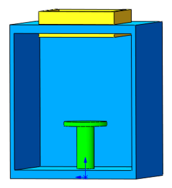
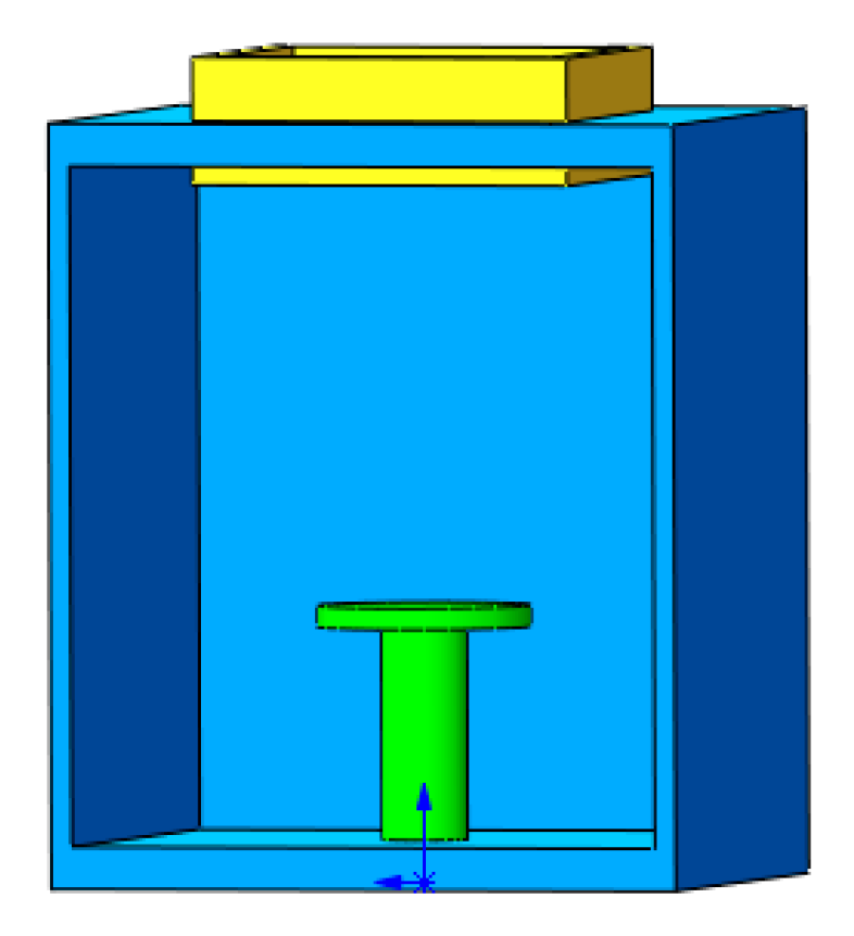
Based on Eidevåg et al. [19], a 3D model was built in SolidWorks 2020. The lower snow collection platform had a diameter D = 50 mm, with the upper snow outlet located H = 100 mm above, as shown in Figure 1.

Figure 1. Simulation experimental device model.

2.2.2. Contact Model Selection

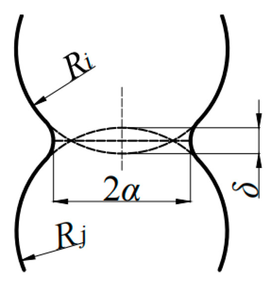
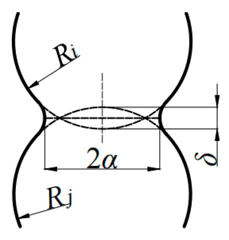
The contact model is central to the DEM. Johnson et al. [22] proposed a Hertz–Mindlin with JKR contact model for adhesive particles in 1971, and the contact model is shown in Figure 2. Although the snow investigated in this study is classified as “dry snow” under −10 °C conditions, this classification refers to a low macroscopic liquid water content rather than the complete absence of liquid water, which gives rise to surface-energy-driven adhesive interactions during particle contact [23]. On this basis, the Hertz–Mindlin contact model with JKR adhesion is adopted in this study.

Figure 2. Hertz–Mindlin with JKR contact model.

Where R_i and R_j are the radius of the contact particles, m; α is the contact radius, m; and δ is the normal deformation, m. Due to the distribution of contact stress, the calculation formula for the total contact normal force is:

$$F_J={\displaystyle \frac{4E^{*}{\alpha }^3}{3R^{*}}}-\sqrt{8\pi {\gamma }^{*}{E}^{*}{\alpha }^3}$$

(2)

where R* is the effective contact radius and the second term is the adhesion component; E* is equivalent Young’s modulus, Pa; γ* is the effective surface energy per unit area, J/m²; and α is the equivalent radius, m.

$$E^{\ast }={\left({\displaystyle \frac{1-{\nu }_1}{2G_1}}+{\displaystyle \frac{1-{\nu }_2}{2G_2}}\right)}^{-1}$$

(3)

where G₁ and G₂ are the shear modulus (MPa) of the two particles and ν₁ and ν₂ are the Poisson‘s ratio of the two particles.

$$R^{\ast }={\left({\displaystyle \frac{1}{R_i}}+{\displaystyle \frac{1}{R_j}}\right)}^{-1}$$

(4)

For different material particles:

$${\gamma }^{\ast }={\gamma }_1+{\gamma }_2-2{\gamma }_{12}$$

(5)

where γ₁ and γ₂ are the surface energies of the two particles, J/m², and γ₁₂ is the interfacial energy, J/m².

When the two granular materials are the same, γ₁ = γ₂ = γ, γ₁₂ = 0, that is, γ* = 2γ. According to JKR theory, the normal deformation δ is calculated as follows:

$$\delta ={\displaystyle \frac{a^2}{R^{*}}}-\sqrt{{\displaystyle \frac{4\pi \gamma \alpha }{E^{\ast }}}}$$

(6)

2.2.3. Particle Scaling Theory

In DEM, particle size can be enlarged to save computation time [24]. Dimensional analysis is employed to ensure physical consistency before and after scaling. Density is a directly measured fundamental parameter. The base dimensions are length (L), density (ρ), and time (T). Let the scaling factor for length and time be h, with density unchanged, that is [25]:

$${\lambda }_L=h,\hspace{1em}{\lambda }_T=h,\hspace{1em}{\lambda }_{\rho }=1$$

(7)

Based on the above settings, the scale factors of other relevant particle characteristic parameters can be derived by dimensional analysis.

For the mass, M:

M = ρL³, then: ${\lambda }_M={\lambda }_L^3=h^3$

According to Newton’s second law:

F = Ma, then: ${\lambda }_F={\lambda }_{\rho }{\lambda }_L^4{\lambda }_T^{-2}=h^2$

From the velocity formula:

v = L/T, then: ${\lambda }_v={\lambda }_L{\lambda }_T^{-1}=1$

Young’s modulus:$E={\displaystyle \frac{FL}{Au}}$, then: ${\lambda }_E={\lambda }_{\rho }{\lambda }_L^2{\lambda }_T^{-2}=1$

Particle stress σ = F/A, then: ${\lambda }_{\sigma }={\lambda }_{\rho }{\lambda }_L^2{\lambda }_T^{-2}=1$

Particle strain ε = σ/E, then: ${\lambda }_{\epsilon }={\displaystyle \frac{{\lambda }_{\sigma }}{{\lambda }_E}}=1$

By transforming Equation (2) into a stress–strain formulation,

$$\sigma (\epsilon ,R^{*})={\displaystyle \frac{F_J}{A}}={\displaystyle \frac{4E^{*}}{3}}{\epsilon }^{{\displaystyle \frac{3}{2}}}-\sqrt{{\displaystyle \frac{8\pi \Delta \gamma E^{*}}{R^{*}}}}{\epsilon }^{{\displaystyle \frac{3}{4}}}$$

(8)

It can be observed that the first term on the right-hand side is scale invariant with respect to particle size. In contrast, the second term originates from the JKR adhesive contact model and explicitly depends on the effective particle radius R*. As a result, the JKR adhesive contribution does not satisfy scale invariance.

Based on the above similarity theory and dimensional analysis, when the particle scaling approach is employed in discrete element simulations, the scaling factors of Young’s modulus, stress, strain, and velocity are equal to unity. This implies that the intrinsic material properties can be preserved after scaling. However, due to the explicit radius dependence of the JKR adhesive term, the parameters associated with the contact model still require calibration to ensure that the discrete element model accurately reproduces the macroscopic flow behavior of snow. In the present study, the particle diameter is scaled from d = 0.55 mm to d = 3.3 mm, corresponding to a geometric scaling factor of six, and the simulation apparatus is scaled accordingly.

2.2.4. Simulation Parameters Setting

DEM parameters include the intrinsic properties of particles and device, contact parameters, and computational settings. These parameters significantly affect both the efficiency and accuracy of the simulation [26]. Inflatable membrane structures typically use PVC film, with ν = 0.45, E = 113 MPa [27], and ρ = 1300 kg/m³ [28].

In DEM, a large time-step may lead to numerical inaccuracies or even instability, while an excessively small time step greatly increases computation time. The timestep is usually 10% to 20% of the Rayleigh timestep, which is calculated as [29]:

$$t_{Ray}={\displaystyle \frac{\pi R}{0.8766+0.163\nu }}\sqrt{{\displaystyle \frac{\rho }{G}}}$$

(9)

where ν is the Poisson’s ratio of the particle material; G is the shear modulus; ρ is the density of the granular material; and R is the radius of the particle.

Lommen et al. [30] found that a G varying between 10 MPa and 100,000 MPa has minimal impact on the repose angle. As Equation (7) shows, a smaller G allows faster simulation. Therefore, to maximize computational efficiency while maintaining accuracy, a shear modulus of G = 10 MPa is adopted for snow particles in this study.

2.3. Simulation Experiment Design

Experimental design is a widely employed methodology in various scientific disciplines for identifying key factors and developing predictive models. In this study, the following three-step approach is employed to identify optimal parameters: Plackett–Burman (P-B) test, steepest ascent, and response surface methodology (RSM). All designs were generated with Design-Expert 11.

Initially, a P-B test is used to distinguish significant factors among seven parameters (X0 to X6), including surface energy, contact parameters, and so on, using repose angle as the response. These parameters characterize the dynamic physical properties of particles in the simulation, and they need to be determined for the discrete element simulation software but cannot be measured directly [31].

Among these parameters, the restitution coefficients are velocity-dependent. Vázquez et al. [32] reported that the terminal velocity of snow particles, with sizes ranging from 0.06 to 3.2 mm, falls between 0.06 and 1.6 m/s. Because the wind speed at the top of the air-supported membrane structure is typically higher, the range for the coefficient of restitution was determined based on a reference terminal velocity of 1.6 m/s. Based on prior research on snow [5,6,21], the ranges of contact parameters are listed in Table 2. In the table, the minimum, maximum, and middle values of the contact parameter ranges are coded as −1, 1, and 0, respectively.

Table 2. Plackett–Burman test parameters and coded levels.

No.	Parameters	Codes
		−1	0	1
X0	Snow particle surface energy	0.080	0.165	0.250
X1	Snow–snow restitution coefficient	0.050	0.125	0.200
X2	Snow–snow static friction coefficient	0.050	0.125	0.200
X3	Snow–snow rolling friction coefficient	0.010	0.030	0.050
X4	Snow–membrane restitution coefficient	0.100	0.200	0.300
X5	Snow–membrane static friction coefficient	0.100	0.200	0.300
X6	Snow–membrane rolling friction coefficient	0.010	0.030	0.050

Then, the steepest ascent direction is determined based on the signs of significant effects, and step sizes are determined from parameter ranges.

Finally, a Central Composite Design (CCD) is used to establish a second-order regression model between significant parameters and the response, yielding the optimal parameter setting that is closest to the real repose angle [33].

3. Results and Analysis

This section presents the simulation results and corresponding analyses. An improved measurement method of the repose angle is first introduced and validated. Subsequently, the results of the Plackett–Burman screening experiment and the steepest ascent test are analyzed to identify significant factors and appropriate parameter ranges. The response surface modeling results, including regression analysis, outlier correction, and ANOVA, are then discussed in detail. Finally, the optimal parameter combination is determined and its physical rationality is examined through comparison with the existing literature.

3.1. Improved Measurement Method of Repose Angle

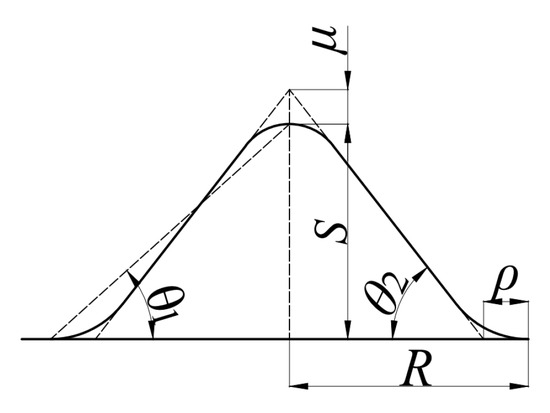
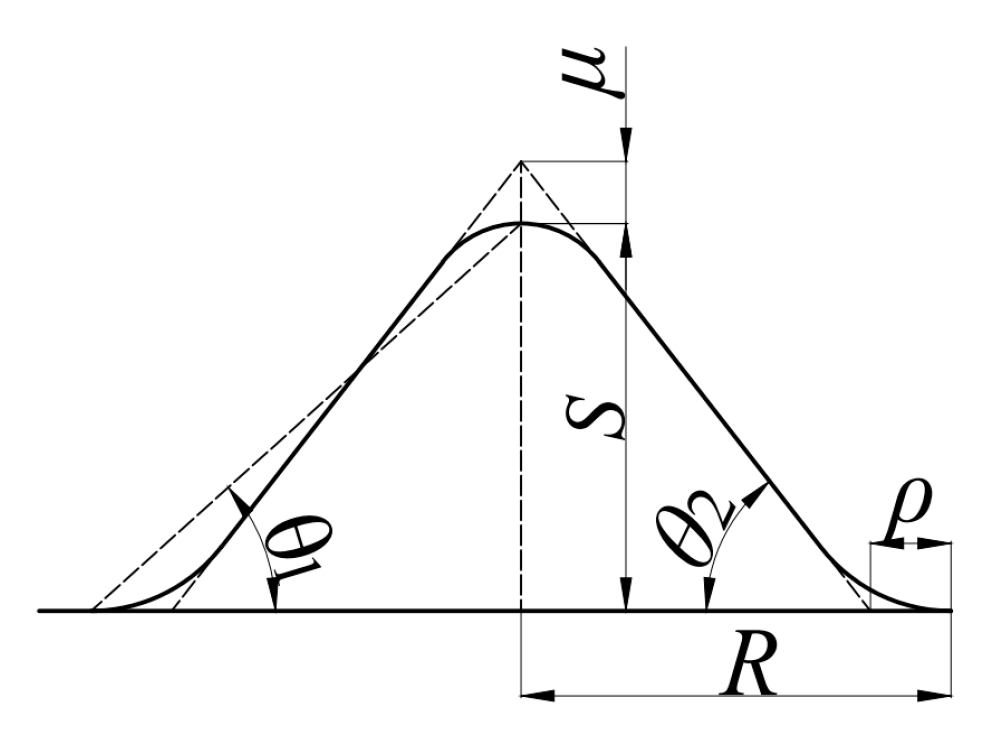
In the actual experimental determination process of the repose angle, the irregular shape formed by the accumulation body of particles often results in the measured repose angle being lower than the true value [8]. The approximate shape of the accumulation body is shown in Figure 3. This shape is a typical contour formed when measuring the repose angle of granular materials by standard experimental methods such as the Funnel Method, which provides controllable and repeatable geometric conditions for parameter calibration [7,8,9,10,11].

Figure 3. Actual accumulation body model.

Here, θ₁ is the measured repose angle; θ₂ is the true repose angle; S is the actual height of the accumulation body; R is the radius of the accumulation body; μ is the height error; and ρ is the radius error.

The expression of the repose angle θ₁ measured by the traditional method is:

$${\tan }^{-1}{\theta }_1={\displaystyle \frac{S}{R}}$$

(10)

The expression of the true repose angle θ₂ is:

$${\tan }^{-1}{\theta }_2={\displaystyle \frac{S+\mu }{R-\rho }}$$

(11)

Due to the existence of height error μ and radius error ρ, the measured value of the repose angle will be smaller than the real value.

To address this issue, a method for measuring the repose angle of accumulation body images is proposed. In the actual accumulation contour, the slope representing the true repose angle is nearly constant, meaning the second derivative within this interval approaches zero. Therefore, according to this law, the interval segment that can express the true repose angle in the polynomial fitting function of the accumulation body contour can be found.

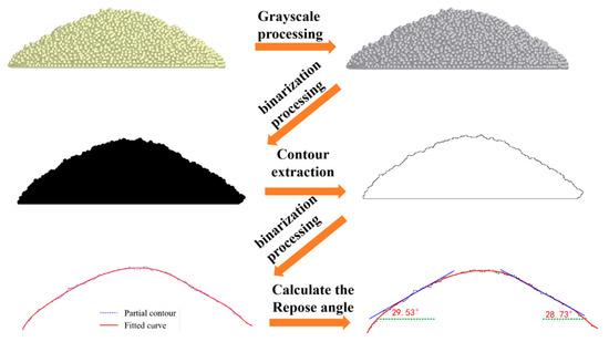
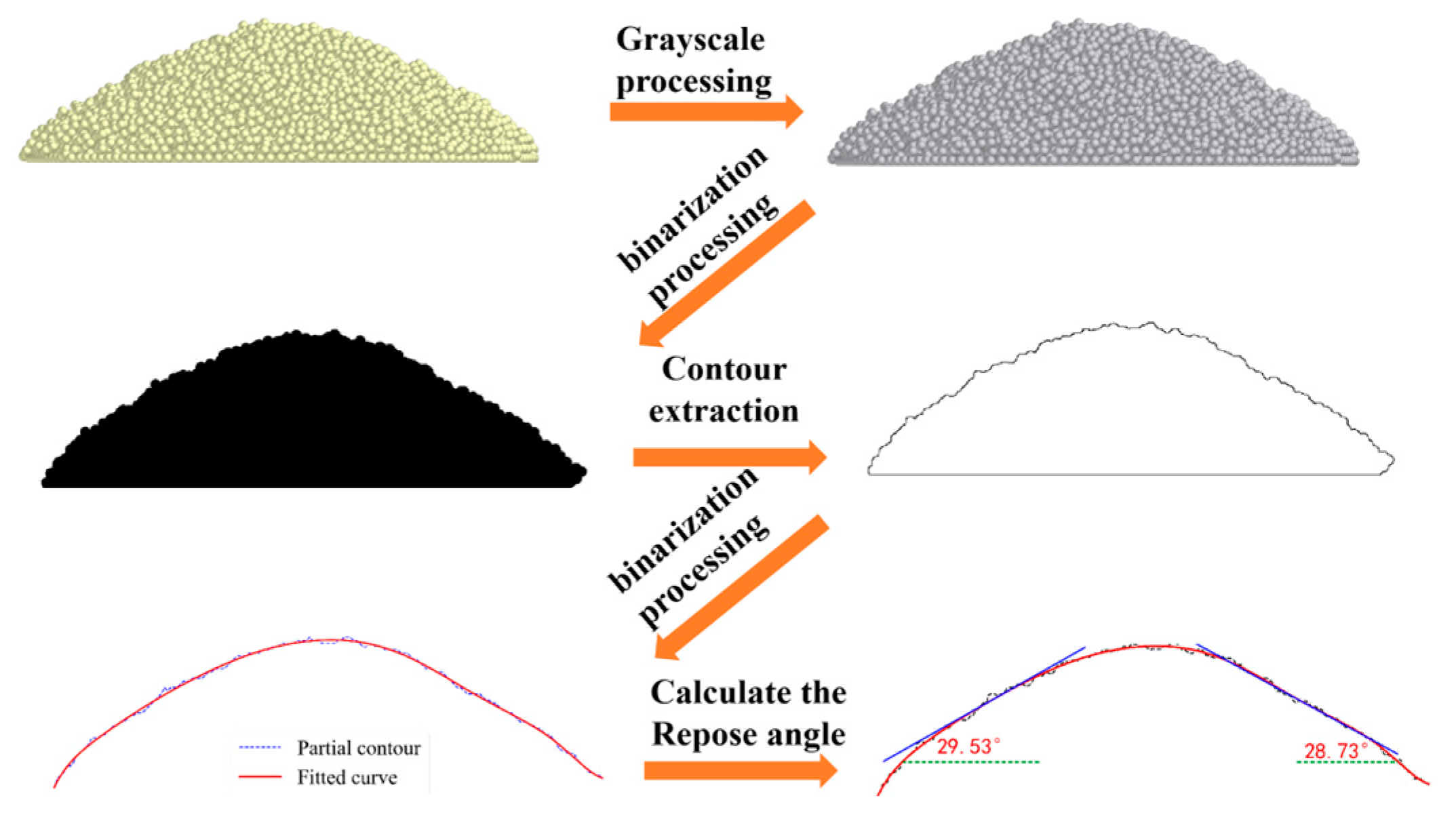
Compared with the method of directly fitting the half-edge contour of the accumulation body with a straight line, the proposed method can not only describe the actual shape of the accumulation body more accurately, but also avoid the interference caused by the irregular contour to a great extent. As shown in Figure 4, the specific operation steps are as follows:

Figure 4. Measurement process of repose angle.

• Read the target image and convert it to grayscale, then apply binarization;
• Detect the pile contour in the binarized image using the Canny operator;
• Crop the contour to retain only the upper slope region and fit it with a polynomial, as shown in Formula (12);

  y = a_nxⁿ + a_n−1xⁿ⁻¹ + ⋯ + a₁x + a₀

  (12)

  where x and y are the horizontal and vertical coordinates of the contour curve.
• Calculate the R² to evaluate the fit and determine the final fitting function;

  $$R^2=1-{\displaystyle \frac{{\displaystyle \sum _{i=1}^n{(y_i-{\widehat{y}}_i)}^2}}{{\displaystyle \sum _{i=1}^n{(y_i-\overline{y})}^2}}}$$

  (13)

  where y_i are the actual values; ${\widehat{y}}_i$ are the values of fitting curve at x_i; $\bar{y}$ are the mean of the actual value; and n is the total number of the data.
• Calculate the second derivative of y, and consider the continuous intervals where the |y″| < ε to be linear intervals;
  where ε reflects the straightness of the interval. After numerous experimental verifications, the test results show that ε = 0.001 yields satisfactorily accurate measurement results.
• In order to ensure that the intervals have physical significance rather than local fluctuations, set the interval where the continuous horizontal distance in the linear interval exceeds 30% of the total width at the bottom of the accumulation body as the effective linear interval. Multiple simulation and experimental results demonstrate that this coverage adequately captures the overall stable geometric characteristics of the pile, and the resulting angle of repose exhibits good robustness against asymmetry and geometric noise.
• In the effective linear intervals, obtain the average value $\bar{k}$ of the first derivative y′ of all points in the ‘effective linear interval’. Then calculate the repose angle θ using Formula (14).

  $$\theta =\left|{\tan }^{-1}\overline{k}\right|$$

  (14)

3.2. Results of the P-B Experiment

Twelve orthogonal tests were designed by Design-Expert 11 and simulated in EDEM 2023.1. The repose angle of each test was measured, as shown in Table 3. The results of the significance analysis are presented in Table 4. In the table, the contribution (%) represents the ratio of the sum of squares of each parameter to the total sum of squares. The rank indicates the relative importance of each parameter, with Rank 1 corresponding to the largest contribution.

Table 3. Designs and results of Plackett–Burman screening experiment.

No.	Parameters							θ/°
	X0	X1	X2	X3	X4	X5	X6
1	−1	−1	−1	1	−1	1	1	31.49
2	−1	−1	1	−1	1	1	−1	30.45
3	−1	1	−1	1	1	−1	1	36.68
4	−1	1	1	1	−1	−1	−1	33.49
5	1	1	−1	1	1	1	−1	43.80
6	1	1	1	−1	−1	−1	1	40.36
7	1	1	−1	−1	−1	1	−1	43.68
8	1	−1	−1	−1	1	−1	1	42.36
9	1	−1	1	1	−1	1	1	36.89
10	−1	1	1	−1	1	1	1	30.63
11	−1	−1	−1	−1	−1	−1	−1	37.29
12	1	−1	1	1	1	−1	−1	37.26

Table 4. Significance analysis of contact parameters based on the contribution to repose angle.

Parameters	Effect	Sum of Square	Contribution%	Ranks
X0	7.39	163.69	63.61	1
X1	2.15	13.87	5.39	3
X2	−4.37	57.29	22.27	2
X3	−0.86	2.22	0.86	6
X4	−0.34	0.34	0.13	7
X5	−1.75	9.19	3.57	4
X6	−1.26	4.76	1.85	5
R2 = 0.9769	$R_{\mathrm{Adj}}^2=0.9365$

3.3. Results of the Steep Climbing Experiment

Significant factors were selected to design the steep climbing experiment. The climbing step size was determined based on the parameter range and the direction of effects, with positive effects leading to an increase and negative effects to a decrease. The other parameters were set at the central levels, namely X3 = 0.03, X4 = 0.2, and X6 = 0.03. The experimental scheme and simulation results are shown in Table 5.

Table 5. The steepest climb test scheme and repose angle results.

No.	Parameters				θ/°
	X0	X1	X2	X5
1	0.08	0.05	0.20	0.30	21.47
2	0.11	0.08	0.17	0.26	24.92
3	0.14	0.11	0.14	0.22	27.65
4	0.17	0.14	0.11	0.18	31.10
5	0.20	0.17	0.08	0.14	36.08
6	0.23	0.20	0.05	0.10	26.68

Among these experiments, the result of No. 5 is the closest to the target angle value (40.75°), so the data of No. 5 are selected as the central level, while No. 4 and No. 6 are, respectively, set as the low-level and high-level values.

3.4. Response Surface Design Results

CCD response surface design was implemented using Design-Expert 11 software. Table 6 presents the experimental factor codes. For a CCD involving k factors, the experimental design consists of three components [33]:

N = 2^k + 2k + n₀

(15)

Table 6. Coded factor levels and actual parameter values.

Codes	Parameters
	X0	X1	X2	X5
2	0.26	0.23	0.14	0.22
1	0.23	0.20	0.11	0.18
0	0.20	0.17	0.08	0.14
−1	0.17	0.14	0.05	0.10
−2	0.14	0.11	0.02	0.06

Here, 2^k represents the number of factorial points, 2k represents the number of axial points, and n₀ represents the number of center points.

For k = 4, the design includes 16 factorial points and 8 axial points to estimate the linear, interaction, and quadratic effects of the response surface. To account for inherent variability in DEM simulations caused by random particle initialization and contact sequencing, 14 replicated center points were included to improve the estimation of pure error and enhance the reliability of the ANOVA. Consequently, a total of 38 experiments were conducted, which is sufficient for constructing and analyzing a four-factor quadratic response surface model while maintaining a reasonable balance between model accuracy and computational cost.

Based on the significant parameters identified in the P-B experiment and the optimal parameter ranges selected in the steepest ascent test, the experimental plan and results are shown in Table 7.

Table 7. CCD test scheme and measured repose angles for four iterative rounds.

No.	Parameters				θ1/(°)	θ2/(°)	θ3/(°)	θ4/(°)
	X0	X1	X2	X5
1	2	0	0	0	40.98	40.98	40.98	40.98
2	2	0	0	0	39.47	39.47	39.47	39.47
3	1	−1	−1	−1	35.40	35.40	35.40	35.40
4	1	1	−1	−1	35.01	35.01	35.01	35.01
5	1	1	1	−1	35.02	36.12	36.12	36.12
6	1	−1	1	1	35.70	35.70	35.70	35.70
7	1	1	−1	1	36.88	36.88	36.88	36.88
8	1	1	1	1	31.88	31.88	31.88	31.88
9	1	−1	1	−1	40.99	40.99	40.99	40.99
10	1	−1	−1	1	41.13	41.13	41.13	41.13
11	0	−2	0	0	38.53	38.53	38.53	38.53
12	0	−2	0	0	36.92	36.92	37.25	37.25
13	0	2	0	0	33.25	33.25	33.25	33.25
14	0	2	0	0	32.82	32.82	32.82	32.82
15	0	0	−2	0	37.43	37.43	37.43	37.43
16	0	0	−2	0	36.34	36.34	36.34	36.34
17	0	0	2	0	36.43	36.43	36.43	36.43
18	0	0	2	0	38.21	38.21	38.21	38.21
19	0	0	0	−2	33.09	33.09	33.09	33.09
20	0	0	0	−2	34.20	34.20	34.20	34.20
21	0	0	0	2	33.24	33.24	33.24	33.24
22	0	0	0	2	34.49	34.49	34.49	34.49
23	0	0	0	0	26.43	25.63	25.63	23.78
24	0	0	0	0	26.37	26.37	25.40	25.40
25	0	0	0	0	20.13	21.23	21.23	21.23
26	0	0	0	0	20.11	20.56	23.46	23.46
27	0	0	0	0	24.31	24.31	24.31	24.31
28	0	0	0	0	26.23	26.23	26.23	22.63
29	−1	1	1	−1	36.17	36.17	36.17	36.17
30	−1	1	−1	1	35.04	35.04	35.04	35.04
31	−1	−1	−1	1	39.78	39.78	39.78	36.17
32	−1	1	−1	−1	31.70	31.70	31.70	31.70
33	−1	−1	1	−1	34.42	34.42	34.42	34.42
34	−1	−1	1	1	35.69	35.69	35.69	35.69
35	−1	1	1	1	30.94	30.94	30.94	30.94
36	−1	−1	−1	−1	32.47	32.47	32.47	32.47
37	−2	0	0	0	31.65	31.65	31.65	31.65
38	−2	0	0	0	30.89	30.89	30.89	30.89

3.4.1. Response Surface Model Construction and the Optimization Method

When designing the response surface, it is usually assumed that y is the quality characteristic of the product or process, that is, the response, and the input variables x₁, x₂, …, x_k have the following relationship:

$$y=f(x_1,x_2,\dots ,x_k)+\epsilon$$

(16)

In the model, there is a random error ε. It is usually assumed that the random errors are independently and normally distributed, i.e., ε ~ N(0, σ²), and the response variable has no measurement error [34]. In practice, measurement errors are inevitable. To ensure the reliability of the prediction and optimization results of the response surface method model, we can optimize the model through residual analysis based on this feature.

First, we calculate the residual ε_i between the predicted value of the regression model and the real data. Then, we construct the reference line function of ε_i through the Q-Q plot [35]; then, outliers are identified through residual analysis. The specific operation steps are as follows:

• Sort the ε_i set from small to large to obtain the sample data set u = {u₁, u₂, …, u_i, …, u_n}, i = 1, 2, …, n, and calculate the theoretical quantile Z_(i) of the data. The formula is [36]:

  $$Z_{(i)}={\mathit{\Phi }}^{-1}\left({\displaystyle \frac{i-0.375}{n+0.25}}\right)$$

  (17)

  where Φ(x) represents the cumulative distribution function of the standard normal distribution; n is the number of sample data; and i is the rank after sorting.
• Construct the reference line function. The formula is:

  $$y_{\left(i\right)}=\sigma Z_{(i)}+\mu$$

  (18)

  where y_(i) represents the theoretical value of the rank i which follows the normal distribution N(μ, σ²); σ is the standard deviation of the sample data.
  $\sigma =\sqrt{{\displaystyle \frac{1}{N}}{\displaystyle \sum _{i=1}^N{\left(u_i-\mu \right)}^2}}$; μ represents the mean value of the sample data. $\mu ={\displaystyle \frac{1}{n}}{\displaystyle \sum _{i=1}^n{u}_i}$.
• Calculate the absolute values of residuals Δ_i for all sample data and their corresponding theoretical values, with the formula being Δ_i = |y(i) − u_i|.
• Calculate the probability density function of the absolute values of residuals Δ_i through Kernel Density Estimation (KDE), which is a nonparametric probability density estimation method, with the formula being [37]:

  $$f(x)={\displaystyle \frac{1}{nh}}{\displaystyle \sum _{i=1}^{n}K\left(\frac{x-{\Delta }_i}{h}\right)}$$

  (19)

  where x is a continuous variable representing the absolute value of residuals and $x\in [{\Delta }_1,{\Delta }_n]$; f(x) is the probability density function; K is the kernel function, and a Gaussian kernel function is selected, $K(x)={\displaystyle \frac{1}{\sqrt{2\pi }h}}{e}^{-x^2/\left(2h^2\right)}$; and h is the bandwidth.
• Calculate the cumulative distribution function F(x) of the absolute value of residuals. The formula is:

  $$F(x)={\displaystyle {\int }_{-\infty }^{{\Delta }_q}f(x)d_x}$$

  (20)

Here, Δ_q represents the threshold for determining outliers.

The confidence level is set to 95%, and the threshold Δ_q is calculated by the cumulative distribution function F(x) = 0.95. If Δ_i ≥ Δ_q, then it is considered that u_i in the original data is an outlier.

We carried out multiple parallel tests on the simulation experimental group corresponding to the residual u_i and took the average value as the correction result. However, the regression equation of Group 1 was obtained in the presence of outliers, so the screened outliers may be incorrectly screened or missed. Therefore, multiple iterations are required until no further outliers are detected.

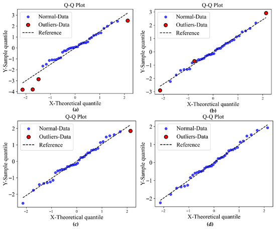
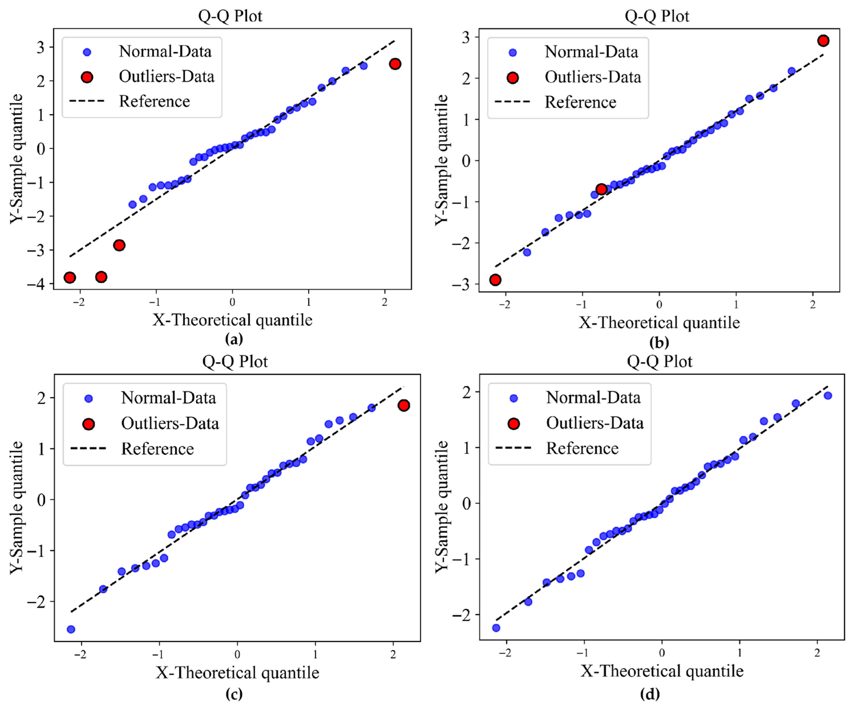
According to the above operation process, this study carried out three iterations on the repose angle data of Group 1 of the response surface design, and finally found no outliers in the residual analysis results of Group 4. The Q-Q plots of the residuals of each group are shown in Figure 5, where the red point represents the abnormal data point, the blue represents the normal data point, and the dotted line represents the reference line of the normal distribution. It can be seen from the diagram that the residuals of Group 4 are almost distributed along the reference line, which strictly conforms to the normal distribution.

Figure 5. Result of outlier screening of Group 1 to Group 4: (a) Q-Q Plot of Group 1. (b) Q-Q Plot of Group 2. (c) Q-Q Plot of Group 3. (d) Q-Q Plot of Group 4.

In Table 7, θ₁ represents the original repose angle data of Group 1, and θ₂, θ₃, and θ₄, respectively, represent the data of Groups 2, 3, and 4 after one, two, and three iterations. The obtained regression coded equations for each group are shown in Table 8. Table 9 shows the residuals between the predicted values of the regression models from Groups 1 to 4 and the real angle of repose data.

Table 8. Coded second-order regression equations for repose angle from four iterative response surface groups.

	Group 1	Group 2	Group 3	Group 4
Constant	23.93	24.06	24.38	24.07
X0	1.610	1.650	1.650	1.650
X1	−1.300	−1.270	−1.290	−1.290
X2	−0.152	−0.1175	−0.1175	−0.1175
X5	0.211	0.1763	0.1763	0.1763
X0X1	−0.370	−0.3012	−0.3013	−0.3013
X0X2	−0.192	−0.1225	−0.1225	−0.1225
X0X5	−0.470	−0.5388	−0.5387	−0.5387
X1X2	−0.165	−0.0963	−0.0963	−0.0962
X1X5	−0.761	−0.8300	−0.8300	−0.8300
X2X5	−1.920	−1.980	−1.980	−1.980
X02	2.960	2.930	2.850	2.930
X12	2.860	2.840	2.780	2.860
X22	3.30	3.270	3.190	3.270
X52	2.460	2.560	2.470	2.550

Table 9. Response surface model residuals of Group 1 to Group 4.

No.	Parameters				Group
	X0	X1	X2	X5	1	2	3	4
1	2	0	0	0	1.99	1.76	1.80	1.79
2	2	0	0	0	0.48	0.25	0.29	0.28
3	1	−1	−1	−1	−1.15	−1.39	−1.41	−1.42
4	1	1	−1	−1	−0.05	−0.26	−0.24	−0.25
5	1	1	1	−1	−2.86	−1.32	−1.30	−1.31
6	1	−1	1	1	−1.49	−1.74	−1.76	−1.77
7	1	1	−1	1	0.02	−0.20	−0.18	−0.19
8	1	1	1	1	−0.12	−0.33	−0.31	−0.32
9	1	−1	1	−1	0.96	0.74	0.72	0.71
10	1	−1	−1	1	−0.26	0.11	0.09	0.08
11	0	−2	0	0	0.56	0.91	0.79	0.78
12	0	−2	0	0	−1.05	−0.70	−0.49	−0.50
13	0	2	0	0	0.48	0.27	0.23	0.22
14	0	2	0	0	0.05	−0.16	−0.20	−0.21
15	0	0	−2	0	0.00	0.40	0.40	0.39
16	0	0	−2	0	−1.09	−0.69	−0.69	−0.70
17	0	0	2	0	−0.40	−0.58	−0.58	−0.59
18	0	0	2	0	1.38	1.20	1.20	1.19
19	0	0	0	−2	−0.26	−0.48	−0.44	−0.45
20	0	0	0	−2	0.85	0.63	0.67	0.66
21	0	0	0	2	−0.95	−0.59	−0.55	−0.56
22	0	0	0	2	0.30	0.66	0.70	0.69
23	0	0	0	0	2.50	2.17	1.85	0.31
24	0	0	0	0	2.44	2.91	1.62	1.93
25	0	0	0	0	−3.80	−2.23	−2.55	−2.24
26	0	0	0	0	−3.82	−2.90	−0.32	−0.01
27	0	0	0	0	0.38	0.85	0.53	0.84
28	0	0	0	0	2.30	−0.83	−1.15	−0.84
29	−1	1	1	−1	1.33	1.12	1.14	1.13
30	−1	1	−1	1	0.10	0.49	0.51	0.50
31	−1	−1	−1	1	1.79	−0.21	−0.23	−0.24
32	−1	1	−1	−1	0.44	0.22	0.24	0.23
33	−1	−1	1	−1	−1.09	−1.33	−1.35	−1.36
34	−1	−1	1	1	1.13	1.50	1.48	1.47
35	−1	1	1	1	0.10	−0.13	−0.11	−0.12
36	−1	−1	−1	−1	1.21	1.57	1.55	1.54
37	−2	0	0	0	−0.90	−0.53	−0.49	−0.50
38	−2	0	0	0	−1.66	−1.29	−1.25	−1.26

3.4.2. ANOVA for Corrected Regression Model

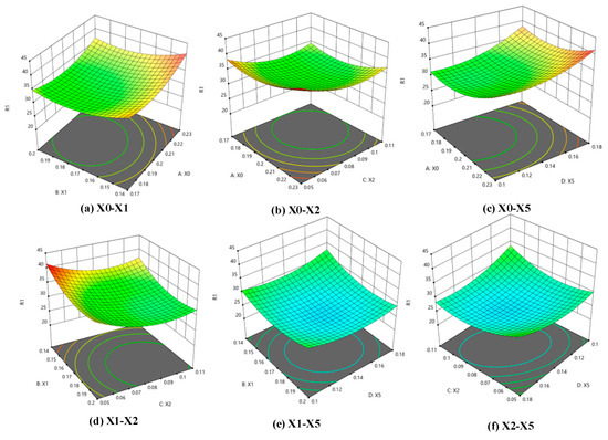
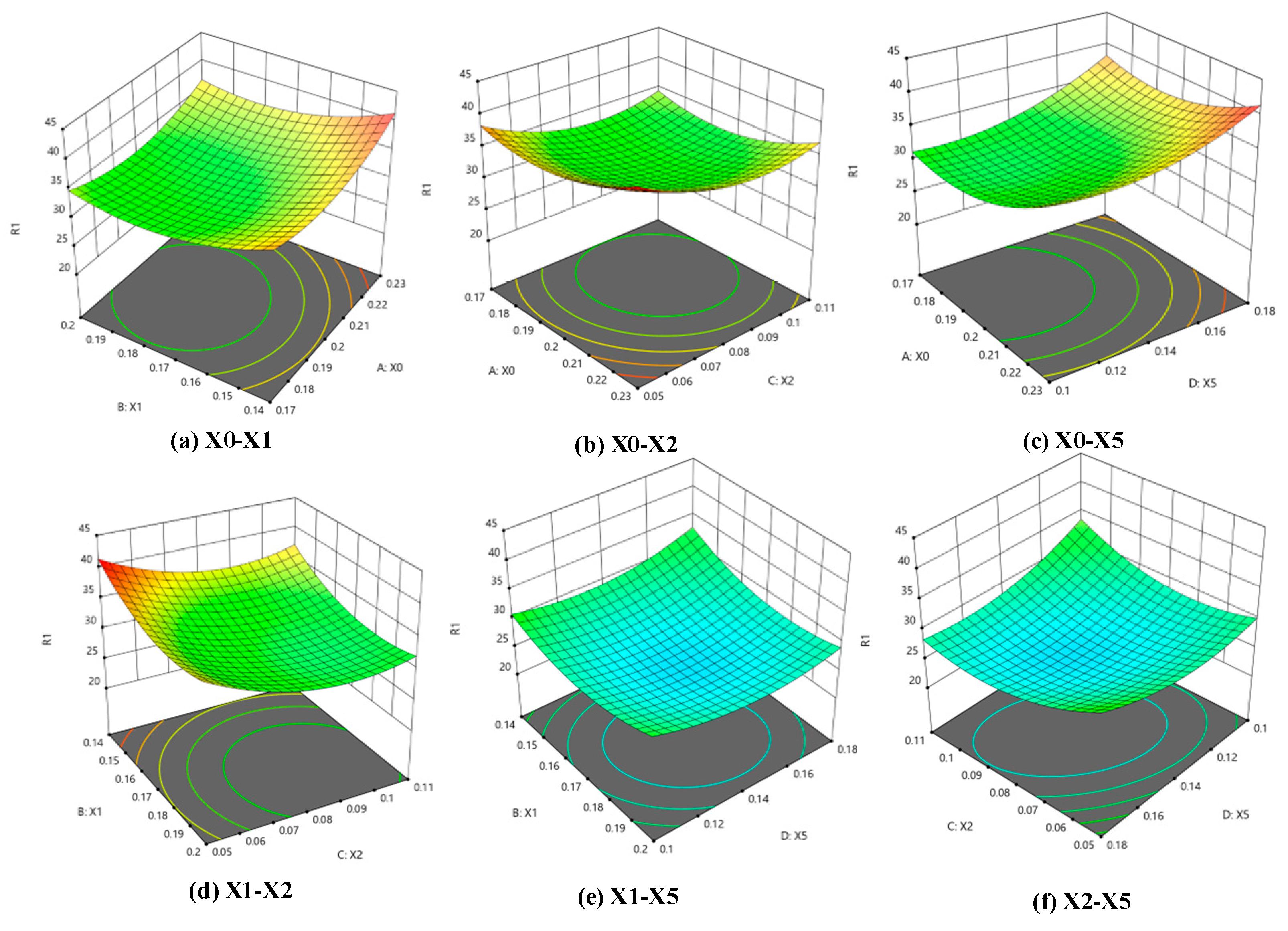
The analysis of variance (ANOVA) was performed on Group 4, and the second-order regression model, as a whole, was very significant (p < 0.0001, R² = 0.9529, $R_{\mathrm{A}\mathrm{d}\mathrm{j}}^2=0.9242$). The lack-of-fit term (p = 0.2445 > 0.05) confirmed the model’s adequacy and absence of systematic bias, with detailed results presented in Table 10. The response surfaces of the interaction between X0 and X1, X2, and X5 are shown in Figure 6.

Table 10. ANOVA for regression model analysis of variance.

Source	Sum of Squares	Degrees of Freedom	Mean Square	F	p
Model	910.71	14	65.05	33.24	<0.0001 **
X0	86.86	1	86.86	44.38	<0.0001 **
X1	53.20	1	53.20	27.19	<0.0001 **
X2	0.4418	1	0.4418	0.2258	0.6392
X5	0.9941	1	0.9941	0.5080	0.4832
X0X1	1.45	1	1.45	0.7420	0.3979
X0X2	0.2401	1	0.2401	0.1227	0.7293
X0X5	4.64	1	4.64	2.37	0.1371
X1X2	0.1482	1	0.1482	0.0757	0.7856
X1X5	11.02	1	11.02	5.63	0.0264 *
X2X5	62.96	1	62.96	32.17	0.00012 **
X02	355.90	1	355.90	181.87	<0.0001 **
X12	338.79	1	338.79	173.12	<0.0001 **
X22	443.02	1	443.02	226.38	<0.0001 **
X52	245.11	1	245.11	125.25	<0.0001 **
Residual	45.01	23	1.96
Lack of Fit	24.08	10	2.41	1.50	0.2445
Pure Error	20.93	13	1.61
Total	955.72	37

Note: * means significant; ** means very significant.

Figure 6. Effects of factor interactions on the repose angle: (a) Interaction between X0 and X1. (b) Interaction between X0 and X2. (c) Interaction between X0 and X5. (d) Interaction between X1 and X2. (e) Interaction between X1 and X2. (f) Interaction between X2 and X5.

In the ANOVA, the terms X2 and X5 are not significant in their linear contributions but are highly significant in the corresponding quadratic terms. This result indicates that the response variable does not vary with the parameters in a simple proportional manner. From a microscopic physical perspective, the macroscopic repose angle of snow particles is governed by the structural stability of the particle contact network and the associated energy dissipation mechanisms, which are coupled during particle deposition and rearrangement processes and collectively determine the stable angle of the accumulation body. When the relevant parameters fall within certain ranges, the particle system may undergo a gradual transition from a friction-dominated contact regime to an adhesion–friction coupled regime. Such a transition induces nonlinear changes in the stability of the contact network and in the pathways of energy dissipation, which manifest at the macroscopic scale as the statistical significance of quadratic terms.

3.4.3. Determination and Verification of Optimal Parameter Combination

In order to obtain the best repose angle parameter combination, the actual average repose angle of 40.75° is taken as the optimization objective to solve the coded equation of Group 4 in Table 8, and the constraint conditions are as follows:

$$\left\{\begin{array}{c}\theta (\mathrm{X}0,\mathrm{X}1,\mathrm{X}2,\mathrm{X}5)=40.75\\ \mathrm{s}.\mathrm{t}.\left\{\begin{array}{c}0.14<\mathrm{X}0<0.26\\ 0.11<\mathrm{X}1<0.23\\ 0.02<\mathrm{X}2<0.14\\ 0.06<\mathrm{X}5<0.22\end{array}\right.\end{array}\right.$$

(21)

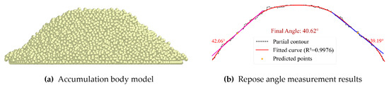
The optimal solution combination of the four significant factors is obtained. The surface energy of snow particles is 0.23 J/m², the snow–snow restitution coefficient is 0.141, the snow–snow static friction coefficient is 0.05, and the snow–membrane static friction coefficient is 0.18. The remaining non-significant factors are selected with intermediate horizontal values, that is, the snow–snow rolling friction coefficient is 0.03, the snow-–membrane restitution coefficient is 0.2, and the snow–membrane rolling friction coefficient is 0.03. The solution results are simulated and verified by EDEM. Using the measurement method in Section 3.1 to calculate the repose angle, Figure 7 illustrates the analysis process and results. Polynomial fitting achieves an R² of 0.9976. This indicates that the measurement results are accurate and reliable.

Figure 7. Simulation result with optimal parameters.

The result shows that left and right repose angles were measured as 42.06° and 39.19°, respectively. The mean value was 40.62°, showing a 0.32% relative error compared to the actual 40.75°, confirming the reliability of the derived contact parameters.

3.4.4. Discussion on the Physical Rationality of the Optimal Parameters

The calibrated parameters are analyzed below to demonstrate their reality and physical plausibility.

Snow–snow restitution coefficient (0.141): This relatively low value indicates significant energy dissipation during collisions, which is consistent with the inelastic deformation and micro-fracture behavior of ice particles under low-velocity impact. Experimental work by Higa et al. [38] showed that for centimeter-sized ice spheres, the coefficient of restitution can rapidly drop below 0.3 in the “inelastic regime” where fracture occurs. Although macroscopic fracture does not occur in our simulations, the energy dissipation mechanisms involved in the numerous collisions during pile formation—such as plastic deformation—are analogous. Therefore, the value of 0.141 is physically reasonable.

Surface energy of snow particles (0.23 J/m²): This parameter governs the adhesive force in the JKR model. For comparison, Boinovich et al. [39] reported a surface energy of approximately 0.122 J/m² for dry snow particles. Our calibrated value of 0.23 J/m² is of the same order of magnitude, confirming the reliability of our result. The discrepancy may stem from our use of a spherical particle model, which effectively accounts for some of the mechanical interlocking effects of real, irregularly shaped snow particles as increased surface adhesion.

Snow–snow static friction coefficient (0.05): Classical work by Israelachvili [40] documents a typical static friction coefficient of about 0.10 for ice–ice contacts, and the sliding friction coefficient is 0.03. The 0.05 calibrated in this study is in between the two, with a minor difference, and is physically realistic.

Snow–membrane static friction coefficient (0.18): The coefficient of friction between typical polymer materials and snow usually falls within the range of 0.1 to 0.3 [41,42,43]. Our experimentally calibrated value of 0.18 for the snow–membrane interface is consistent with these known frictional characteristics of snow–polymer contacts.

Regarding the three parameters identified as non-significant in the Plackett–Burman test: The snow–snow rolling friction coefficient of 0.03 aligns with the low rolling resistance typically exhibited by dry granular materials like snow, where energy dissipation via rolling is considerably smaller than that via static or sliding friction. The snow–membrane restitution coefficient of 0.2 indicates a moderately inelastic collision, which is physically reasonable for impacts between snow particles and a deformable polymer membrane, as energy is dissipated through material damping and plastic deformation at the contact point. The snow–membrane rolling friction coefficient of 0.03 is a low value, consistent with the minimal rolling resistance expected on a smooth membrane surface.

Table 11 summarizes the calibrated contact parameters obtained in this study and compares them with the physically reasonable ranges reported in the literature on snow particle properties, together with the corresponding data sources and references. The comparison demonstrates that all seven calibrated parameters fall within well-established physical ranges and exhibit clear physical significance, confirming their suitability as a reliable parameter set for subsequent discrete element simulations.

Table 11. Comparison between the calibrated DEM contact parameters obtained in this study and the ranges reported in the literature.

Parameter	Calibrated Value	Reported Value	References
Snow–snow restitution coefficient	0.141	0.1–0.3	[38]
Surface energy of snow particles	0.23 J/m2	0.122 J/m2	[39]
Snow–snow static friction coefficient	0.05	0.03–0.1	[40]
Snow–membrane static friction coefficient	0.18	0.1–0.3	[41,42,43]
Snow–snow rolling friction coefficient	0.03	0.03–0.1	[40]
Snow–membrane restitution coefficient	0.2	0.1–0.3	[41,42,43]
Snow–membrane rolling friction coefficient	0.03	0.01–0.05	[41,42,43]

It should be noted that the inverse identification of DEM contact parameters based on a single macroscopic response may inherently involve a degree of non-uniqueness. The objective of this study is not to seek a mathematically unique solution, but to obtain a physically consistent and statistically reliable parameter set that can accurately reproduce the macroscopic flow behavior of snow particles in discrete element simulations.

4. Conclusions

This study establishes a physically grounded and statistically robust calibration framework for discrete element modeling of snow, and the main findings can be summarized as follows:

(1) Through a Plackett–Burman (P–B) screening design, four contact parameters were identified as statistically significant factors governing the angle of repose of snow particles, namely the surface energy of snow particles, the snow–snow static friction coefficient, the snow–snow restitution coefficient, and the snow–membrane static friction coefficient. This result clarifies the dominant microscopic parameters controlling macroscopic pile stability under the investigated conditions.

(2) An image-based angle-of-repose measurement method was proposed based on polynomial fitting of the complete pile outline. Unlike conventional approaches relying on limited local slopes, the proposed method utilizes the full contour information of the granular pile, thereby improving the robustness and accuracy of repose angle estimation in the presence of geometric irregularities and particle-scale fluctuations.

(3) A response surface optimization framework incorporating Q–Q plot reference line construction and residual-based outlier treatment was established. By iteratively correcting error-prone data points through repeated simulations rather than direct exclusion, the reliability and statistical consistency of the response surface model were significantly improved.

(4) Based on the optimized second-order regression model, a physically consistent set of DEM contact parameters was obtained. The calibrated values included a snow surface energy of 0.23 J/m², a snow–snow restitution coefficient of 0.141, a snow–snow static friction coefficient of 0.05, and a snow–membrane static friction coefficient of 0.18, while intermediate values were retained for the remaining parameters. Using this parameter set, the simulated angle of repose reached 40.62°, corresponding to a relative error of only 0.32% compared with the experimental reference value of 40.75°. These results demonstrate that the proposed calibration strategy is both statistically sound and physically meaningful for reproducing the macroscopic flow behavior of snow.

In future studies, the calibrated contact parameters will be applied to discrete element method (DEM) simulations of snow removal robots operating on membrane structures. The DEM framework will be used to quantitatively predict the snow removal performance of the robot, as well as the accumulation, adhesion, and flow behavior of snow during the removal process. Based on these simulation results, key components of the snow removal robot—such as the geometry of the snow pusher, the design of the snow-blowing pipeline, and the overall system layout—can be systematically optimized.

References

- Zhang, A.Y.; He, J.H. The impact of climate change on crop growth and countermeasures. Rural Sci. Technol. Exp. 2025, 5, 193–195. [Google Scholar] [CrossRef]
- Xiang, Y.; Li, Y.; Yu, P.B.; Wang, Y.; Tang, Y.; Xue, F.; Zhuang, X.N.; Liu, J. Innovative development and engineering design application optimization of grain air-film warehouses. Grain Storage 2024, 53, 1–5+16. [Google Scholar]
- Li, M.S.; Wang, Y.J.; Xie, S.Y.; Liu, Y.F.; Chen, X.Z.; Li, X.; Liu, W. Simulation and experimental analysis of the operational performance of deep-loosening machines based on discrete element method. Trans. Chin. Soc. Agric. Eng. 2024, 40, 81–90. [Google Scholar] [CrossRef]
- Johnson, J.B.; Hopkins, M.A. Identifying microstructural deformation mechanisms in snow using discrete-element modeling. J. Glaciol. 2005, 51, 432–442. [Google Scholar] [CrossRef] [Scilit]
- Bobillier, G.; Bergeld, B.; Capelli, A.; Dual, J.; Gaume, J.; Van Herwijnen, A.; Schweizer, J. Micromechanical modeling of snow failure. Cryosphere 2020, 14, 39–49. [Google Scholar] [CrossRef] [Scilit]
- Hagenmuller, P.; Chambon, G.; Naaim, M. Microstructure-based modeling of snow mechanics: A discrete element approach. Cryosphere 2015, 9, 1969–1982. [Google Scholar] [CrossRef] [Scilit]
- Zhao, Z.H.; Wu, M.L.; Xie, S.P.; Luo, H.F.; Li, P.C.; Zeng, Y.; Jiang, X.H. Discrete element simulation parameter calibration of soil-rice rotation and its rotary tillage trajectory analysis. Trans. Chin. Soc. Agric. Eng. 2024, 40, 72–82. [Google Scholar] [CrossRef]
- Gao, X.Y.; Wu, P.; Li, X.Z.; Du, H.J.; Wang, W.C.; Wan, Q.H. Research on the repose angle test of granular feed based on MATLAB. J. Agric. Mech. Res. 2024, 46, 173–179. [Google Scholar] [CrossRef]
- Zhang, H.Z.; Liu, Z.M.; Jiang, W.L.; Zhang, X.; Wu, Y. Discrete element parameter calibration of irregular metal powder flow. Metall. Mater. 2024, 44, 22–24. [Google Scholar]
- Chen, S.; Jiang, L.J.; Lin, X.S.; Tang, X.M.; Liu, X.M.; Zhang, L. Calibration of contact parameters for flour particles based on the discrete element method. Trans. Chin. Soc. Agric. Eng. 2024, 40, 69–76. [Google Scholar] [CrossRef]
- Zou, Y.; Tang, T.; Gao, Z.C.; Qiao, Z.D.; Hu, Y.B. Discrete element parameter calibration of quicklime powder based on particle scaling theory. China Powder Technol. 2023, 29, 81–91. [Google Scholar] [CrossRef]
- Fierz, C.; Armstrong, R.L.; Durand, Y.; Etchevers, P.; Greene, E.; McClung, D.M.; Nishimura, K.; Satyawali, P.K.; Sokratov, S.A. The International Classification for Seasonal Snow on the Ground; IACS Contribution No. 1; UNESCO-IHP: Paris, France, 2009; pp. 4–13. [Google Scholar]
- Wang, E.L.; Fu, X.; Han, H.W.; Liu, X.C.; Xiao, Y.; Leng, Y.P. Study on the mechanical properties of compacted snow under uniaxial compression and analysis of influencing factors. Cold Reg. Sci. Technol. 2021, 182, 103215. [Google Scholar] [CrossRef] [Scilit]
- Zermatten, E.; Schneebeli, M.; Arakawa, H.; Steinfeld, A. Tomography-based determination of porosity, specific area and permeability of snow and comparison with measurements. Cold Reg. Sci. Technol. 2014, 97, 33–40. [Google Scholar] [CrossRef] [Scilit]
- Lieblappen, R.; Fegyveresi, J.M.; Courville, Z.; Albert, D.G. Using ultrasonic waves to determine the microstructure of snow. Front. Earth Sci. 2020, 8, 34. [Google Scholar] [CrossRef] [Scilit]
- Arakawa, H.; Izumi, K.; Kawashima, K.; Kawamura, T. Study on quantitative classification of seasonal snow using specific surface area and intrinsic permeability. Cold Reg. Sci. Technol. 2009, 59, 163–168. [Google Scholar] [CrossRef] [Scilit]
- Duan, J.; Guo, H.; Hu, J.R.; Zhou, X.; Wu, X.; Chen, B.J. Research advances on observation and shape classification of natural snow and ice crystal particles. Acta Meteorol. Sin. 2023, 81, 685–701. [Google Scholar] [CrossRef]
- Eidevåg, T.; Abrahamsson, P.; Eng, M.; Rasmuson, A. Modeling of dry snow adhesion during normal impact with surfaces. Powder Technol. 2020, 361, 1081–1092. [Google Scholar] [CrossRef] [Scilit]
- Eidevåg, T.; Thomson, E.S.; Kallin, D. Angle of repose of snow: An experimental study on cohesive properties. Cold Reg. Sci. Technol. 2022, 194, 103470. [Google Scholar] [CrossRef] [Scilit]
- Zhang, X.L.; Wang, H.D.; Xiao, P.F.; Zheng, Z.X.; Feng, X.Z. Electronic atlas of spatiotemporal distribution of snow characteristics in China. China Sci. Data 2022, 7, 24–37. [Google Scholar] [CrossRef]
- Choi, Y.B.; Kim, R.W.; Lee, I.B. Numerical analysis of snow distribution on greenhouse roofs using CFD–DEM coupling method. Biosyst. Eng. 2024, 237, 196–213. [Google Scholar] [CrossRef] [Scilit]
- Johnson, K.L.; Kendall, K.; Roberts, A.D. Surface energy and the contact of elastic solids. Proc. R. Soc. A-Math. Phys. Eng. Sci. 1971, 324, 301–313. Available online: https://www.jstor.org/stable/78058 (accessed on 3 January 2026). [CrossRef] [Scilit]
- Robert, R. Why Is Ice Slippery? Phys. Today 2005, 12, 50–55. [Google Scholar] [CrossRef] [Scilit]
- Zhao, T.T.; Feng, Y.T. Accurate scaling and coarse-graining discrete element methods for large-scale granular systems. Chin. J. Comput. Mech. 2022, 39, 365–372. [Google Scholar] [CrossRef]
- Wang, Q.Z.; Yang, M.; Xiang, J.T.; Zhang, Q.L.; Zhang, W.J.; Li, X.J.; Hu, J.M. Calibration of discrete element parameters for seabuckthorn tea hairs based on particle scaling theory. Agric. Res. Arid Areas 2024, 42, 284–292. [Google Scholar] [CrossRef]
- Coetzee, C.J. Review: Calibration of the discrete element method. Powder Technol. 2017, 310, 104–142. [Google Scholar] [CrossRef] [Scilit]
- Zhang, H.X. Response Analysis of Pneumatic Membrane Structures Under Wind and Rain Loads. Master’s Thesis, Hebei University of Science and Technology, Shijiazhuang, China, 2019. [Google Scholar]
- Liu, Q. Research on Snow Removal of Membrane Structures Based on Thermal Melting Method. Master’s Thesis, Harbin Institute of Technology, Harbin, China, 2022. [Google Scholar]
- Washino, K.; Chan, E.L.; Miyazaki, K.; Tsuji, T.; Tanaka, T. Time step criteria in DEM simulation of wet particles in viscosity dominant systems. Powder Technol. 2016, 302, 100–107. [Google Scholar] [CrossRef] [Scilit]
- Lommen, S.; Schott, D.; Lodewijks, G. DEM speedup: Stiffness effects on behavior of bulk material. Particuology 2014, 12, 107–112. [Google Scholar] [CrossRef] [Scilit]
- Li, M.; He, X.; Zhu, G.; Liu, J.; Gou, K.; Wang, X. Modeling and Parameter Calibration of Morchella Seed Based on Discrete Element Method. Appl. Sci. 2024, 14, 11134. [Google Scholar] [CrossRef] [Scilit]
- Vázquez-Martín, S.; Kuhn, T.; Eliasson, S. Shape dependence of snow crystal fall speed. Atmos. Chem. Phys. 2021, 21, 7545–7565. [Google Scholar] [CrossRef] [Scilit]
- Myers, R.H.; Montgomery, D.C.; Anderson-Cook, C.M. Response Surface Methodology: Process and Product Optimization Using Designed Experiments, 4th ed.; John Wiley & Sons: Hoboken, NJ, USA, 2016; pp. 273–307. [Google Scholar]
- Fang, J.T. Comparative Study on Experimental Design and Model Estimation in Response Surface Methodology. Master’s Thesis, Tianjin University, Tianjin, China, 2011. [Google Scholar]
- Weine, E.; McPeek, M.S.; Abney, M. Application of equal local levels to improve Q-Q plot testing bands with R package qqconf. J. Stat. Softw. 2023, 106, 1–27. [Google Scholar] [CrossRef] [Scilit]
- Li, Y.M. Methods for normality test of data. J. Huaihua Univ. 2015, 34, 81–82. [Google Scholar] [CrossRef]
- Rakhi; Gupta, B.; Lamba, S.S. An efficient local outlier detection approach using kernel density estimation. Franklin Open 2024, 8, 100162. [Google Scholar] [CrossRef] [Scilit]
- Higa, M.; Arakawa, M.; Maeno, N. Size dependence of restitution coefficients of ice in relation to collision strength. Icarus 1998, 133, 310–320. [Google Scholar] [CrossRef] [Scilit]
- Boinovich, L.; Emelyanenko, A. Experimental determination of the surface energy of polycrystalline ice. Dokl. Phys. Chem. 2015, 459, 198–202. [Google Scholar] [CrossRef] [Scilit]
- Israelachvili, J.N. Intermolecular and Surface Forces, 3rd ed.; Academic Press: Waltham, MA, USA, 2011; pp. 471–474. [Google Scholar]
- Klapproth, C.; Kessel, T.M.; Wiese, K.; Wies, B. An advanced viscous model for rubber-ice-friction. Tribol. Int. 2016, 99, 169–181. [Google Scholar] [CrossRef] [Scilit]
- Bäurle, L.; Kaempfer, T.U.; Szabó, D.; Spencer, N.D. Sliding friction of polyethylene on snow and ice: Contact area and modeling. Cold Reg. Sci. Technol. 2007, 47, 276–289. [Google Scholar] [CrossRef] [Scilit]
- Tan, T.; Xing, C.; Tan, Y.Q. Rubber friction on icy pavement: Experiments and modeling. Cold Reg. Sci. Technol. 2020, 174, 103022. [Google Scholar] [CrossRef] [Scilit]
Disclaimer/Publisher’s Note: The statements, opinions and data contained in all publications are solely those of the individual author(s) and contributor(s) and not of MDPI and/or the editor(s). MDPI and/or the editor(s) disclaim responsibility for any injury to people or property resulting from any ideas, methods, instructions or products referred to in the content. |
© 2026 by the authors. Licensee MDPI, Basel, Switzerland. This article is an open access article distributed under the terms and conditions of the Creative Commons Attribution (CC BY) license.