Multi-Fidelity Data and Prior-Enhanced Physics-Informed Neural Networks for Multi-Parameter Identification of Prestressed Concrete Beams with Unquantifiable Noise

Abstract

Although PINNs have demonstrated strong predictive capabilities in forward problems, their performance in inverse problems remains inadequate, largely due to unquantifiable noise encountered during the multi-parameter identification of prestressed concrete beams. Experimental measurements are often noisy, sparse, or asymmetric, while numerical or analytical models, although physically consistent, are typically approximate and lack regularization from well-defined multi-fidelity data. To address this limitation, this paper proposed a multi-fidelity data and prior-enhanced physics-informed neural network (MF-rPINN), which integrates multi-fidelity data with physics prior relational constraints to guide parameter identification using only sparse experimental observations. The MF-rPINN architecture is designed to enforce consistency between each training iteration and a prescribed set of experimental measurements, while embedding the second-order displacement function into the loss function. Experimental results demonstrate that the proposed MF-rPINN achieves accurate parameter identification even under noisy and incomplete observations, owing to the combined regularization effects of governing physical laws and the second-order displacement prior. The minimum relative errors of the elastic modulus are −6.49% and −9.32% under different and identical loading conditions, respectively, while the minimum relative errors of the prestress force are 0.65% and 4.51%. Compared with classical analytical approaches, MF-rPINN exhibits superior robustness and is capable of predicting continuous displacement fields of prestressed concrete beams while simultaneously identifying prestress force and elastic modulus. These advantages highlight the potential of MF-rPINN as a reliable surrogate modeling tool for practical engineering applications.

1. Introduction

1.1. Literature Review

Partial differential equations (PDEs) are fundamental tools for modeling and analyzing both natural and engineered complex systems, as they encapsulate the governing physical principles underlying system behavior [1]. Over recent decades, the solution of multiphysics problems—ranging from geophysics to biophysics—has predominantly relied on analytical and numerical methods. Analytical approaches offer several advantages, including exact solutions, strong generalizability, benchmark references for numerical schemes, and high computational efficiency for small-scale problems [2]. However, many practical problems involving complex geometries, strong nonlinearities, or high-dimensional parameter spaces are not amenable to analytical treatment, rendering numerical methods the only feasible option [3].

Despite significant progress in numerical discretization techniques for PDE-based multiphysics simulations, conventional numerical methods still suffer from notable limitations. These include high computational cost, multiple sources of uncertainty, challenges in mesh generation, and difficulties in handling high-dimensional parameterized PDEs [4]. Moreover, most numerical solvers are primarily designed for forward problems, whereas inverse problems—commonly encountered in engineering and experimental sciences—remain substantially more challenging. Inverse problem formulations often involve increased mathematical complexity, higher computational demands, and pronounced sensitivity to uncertainty [5]. More critically, many real-world engineering and experimental tasks inherently require inverse identification under conditions of missing, incomplete, or noisy data, for which traditional numerical approaches are frequently infeasible [6].

Physics-informed neural networks (PINNs) have recently emerged as a promising paradigm for addressing PDE-governed problems, particularly in inverse settings involving nonlinearities [7,8]. By embedding governing equations directly into the loss function through automatic differentiation, PINNs enable the simultaneous integration of physical laws and sparse observational data within a unified learning framework [9,10,11,12]. This physics-informed training strategy has demonstrated notable potential for solving PDE-based problems in engineering and experimental sciences, where data are often limited or partially observed [13,14,15]. Nevertheless, the effectiveness of PINNs in practical inverse problems is strongly influenced by the availability and quality of training data.

In many scientific and engineering applications, accurate system identification relies on high-fidelity (HF) data, which capture physically meaningful system states but are often expensive to obtain [16,17]. Processing HF data using conventional numerical simulations—especially for high-dimensional and nonlinear problems—typically requires extensive spatial discretization, time stepping, and iterative solution procedures [18,19]. As problem scale increases, these iterative solvers may become prohibitively time-consuming, particularly when numerical conditioning deteriorates or solver efficiency is limited [16].

To alleviate these challenges, multi-fidelity (MF) modeling has been widely adopted since the early 2000s as an effective strategy for balancing computational cost and predictive accuracy [20]. MF modeling leverages the complementary strengths of low-fidelity (LF) and HF data, where LF data are relatively inexpensive but less accurate, while HF data are accurate yet scarce [18]. By exploiting the correlation between LF and HF data, MF approaches can achieve high predictive accuracy with a limited amount of HF information, outperforming single-fidelity models [21,22]. The primary objective of MF modeling is therefore to establish an optimal trade-off between accuracy and affordability [23,24,25].

Connections between LF and HF models are commonly attributed to factors such as dimensionality reduction [26,27], grid coarsening [28], linearization [29], partial convergence [30], reduced geometric complexity [31,32], and simplified physical representations [25]. MF methods have been extensively applied in fluid and solid mechanics, particularly for optimization and uncertainty quantification. In fluid mechanics, fidelity levels may range from analytical expressions and empirical correlations to numerical linear approximations and Euler-based models [33,34]. In solid mechanics, fidelity is often associated with mesh resolution, material modeling, and structural features [35], as well as distinctions between experimental and numerical data or between coarse and refined simulations [36]. Despite these advances, MF modeling still faces challenges in handling discontinuous functions, high-dimensional problems, and strongly nonlinear inverse problems governed by nonlinear PDEs [37]. These limitations motivate the development of MF strategies capable of robust inverse identification under realistic conditions.

Integrating MF modeling with PINNs provides a natural pathway to extend PINN-based methods toward real-world engineering and experimental applications. PINNs have already demonstrated success in diverse domains, including high-speed aerodynamic flows [38], incompressible laminar and turbulent flows [39], solutions of the Fokker–Planck equation [40,41], parameter identification in multiphase thermo-hydro-mechanical processes [41], and fatigue life prediction [42]. Moreover, transfer-learning-based optimization strategies have been proposed for scenarios where the governing physics is only approximately known (LF physics) and HF data are scarce [43,44,45,46]. The combination of such strategies with PINNs has yielded promising results in MF problems, such as phase-field fracture modeling [35] and structural response prediction under varying loading conditions [47].

In parallel, several extended PINN frameworks have been proposed to enhance scalability and efficiency, including INNs [48], FBPINN [49], XPINN [50], PPINN [51], and Δ-PINN [52], along with practical solvers such as NVIDIA SIMNET [53] and NeuralIUQ [54]. And the PINN framework is potentially applicable to other engineering domains characterized by heterogeneous data and partial physical knowledge [55]. One representative example is automated fault detection [56] and diagnosis for air handling units [57], where operational data, physical models, and empirical rules coexist but cannot be strictly ranked by fidelity. Task-based priors within PINN could encode physical constraints or fault signatures, enabling robust inverse identification under noisy and incomplete measurements.

1.2. Scope and Outline

Although PINN and their multi-fidelity extensions have demonstrated strong performance in forward problems, their application to inverse identification in engineering systems remains fundamentally challenging. Classical multi-fidelity PINN frameworks typically assume a clear and quantifiable hierarchy between low- and high-fidelity data sources, where higher-fidelity data are expected to be closer to physical truth. However, in practical engineering inverse problems, this assumption is often violated: experimental measurements may be noisy, sparse, or asymmetric, while numerical or analytical models may be physically consistent yet only approximate. Therefore, in contrast to the domains of mathematics and physics where delineation of data fidelity is relatively straightforward, establishing such precision within the engineering realm becomes challenging despite the authenticity and exactitude of the data. Particularly, the resolution of inverse problems necessitates guidance from a flexible data scale, yet the presence of noise may mislead PINN towards erroneous predictive outcomes. It is noteworthy that deviations from physical intuition, specifically the discrepancies between observational measurements and prior laws, are not necessarily attributable to artificial or engineering noise. Instead, they may indicate internal structural damage or as yet undiscovered laws. Therefore, it is essential to assimilate these MF data in actual engineering and experimental science tasks.

The proposed MF-rPINN framework departs from this conventional fidelity hierarchy. Instead of enforcing a strict classification of low- and high-fidelity data, MF-rPINN treats heterogeneous information, including observational measurements, governing equations, and task-based prior relations, as engineering-domain multi-fidelity data. Their relative credibility is encoded through task-oriented loss weighting rather than predefined fidelity levels. Algorithmically, MF-rPINN introduces an enhanced relation function that acts as a soft identifiability regularization, restricting the inverse solution space to physically admissible regimes without imposing hard constraints. This conceptual shift distinguishes MF-rPINN from existing MF-PINN and prior-enhanced PINN approaches and is particularly suited for inverse problems characterized by non-closure and non-uniqueness.

The main novel contributions of this work are summarized as follows:

(1)

A new loss term was formulated within the PINN framework and instantiated through the second-order displacement function.

(2)

The concept of MF data and its associated data loss was redefined to distinguish engineering-domain observational measurements from additional data required by the PINN formulation.

(3)

A surrogate model was established for the multi-parameter identification of prestressed concrete beams with unquantifiable noise.

(4)

The continuous displacement field of the prestressed concrete beam was predicted, and the prestress force as well as the elastic modulus were simultaneously identified.

The rest of the paper is organized as follows: the key concepts of MF-rPINN are presented in Section 2. The results are shown in Section 4, while problem setup is given in Section 3. Finally, MF-rPINN is discussed (Section 5), and a summary for this work is given in Section 6.

2. Methodology

2.1. Physics-Informed Neural Networks

Consider a parametric partial differential equation defined over a spatial domain Ω, in which the solution u(x, t) depends on a set of parameters λ:

$$\begin{array}{c}f\left(x;{\displaystyle \frac{\mathsf{\partial }u}{\mathsf{\partial }{x}_1}},\cdots ,{\displaystyle \frac{\mathsf{\partial }u}{\mathsf{\partial }{x}_d}};{\displaystyle \frac{{\mathsf{\partial }}^{2}u}{\mathsf{\partial }{x}_1\mathsf{\partial }{x}_1}},\cdots ,{\displaystyle \frac{{\mathsf{\partial }}^{2}u}{\mathsf{\partial }{x}_1\mathsf{\partial }{x}_d}};\cdots ;\lambda \right)=0\\ x=\left(x_1,\cdots ,x_d\right)\in \Omega \end{array},$$

(1)

with the boundary conditions

$$\mathcal{B}\left(u,x\right)=0 \mathrm{on} \mathsf{\partial }\Omega .$$

Within the PINN framework, the unknown solution is approximated by a neural network û(x; θ) parameterized by trainable weights θ. Model training is driven by enforcing the governing equation and boundary constraints through a set of collocation points sampled from the interior of the domain and its boundary. Let C_f denote the collocation points and C_b the boundary points. The corresponding objective function is constructed as a weighted combination of the residuals:

$$L\left(\theta ;C\right)=w_f{L}_f\left(\theta ;C_f\right)+w_b{L}_b\left(\theta ;C_b\right),$$

(2)

where

$$\left\{\begin{array}{l}{L}_f\left(\theta ;C_f\right)={\displaystyle \frac{1}{\left|C_f\right|}}\times {{\displaystyle {\sum }_{x\in C_f}\left|f\left(x;\frac{\mathsf{\partial }\widehat{u}}{\mathsf{\partial }{x}_1},\cdots ,\frac{\mathsf{\partial }\widehat{u}}{\mathsf{\partial }{x}_d};\frac{{\mathsf{\partial }}^2\widehat{u}}{\mathsf{\partial }{x}_1\mathsf{\partial }{x}_1},\cdots ,\frac{{\mathsf{\partial }}^2\widehat{u}}{\mathsf{\partial }{x}_1\mathsf{\partial }{x}_d};\cdots ;\lambda \right)\right|}}^2\\ L_b\left(\theta ;C_b\right)={\displaystyle \frac{1}{\left|C_b\right|}}{{\displaystyle {\sum }_{x\in C_b}\left|B\left(\Delta \widehat{u},x\right)\right|}}^2\end{array}\right.,$$

and w_f and w_b control the relative importance of each constraint.

A key feature of PINNs is their ability to address inverse problems within the same optimization framework. When the parameter λ is unknown, additional observations of the solution field are incorporated at a set of measurement points C_m. In this case, both the network parameters and the physical parameters are optimized simultaneously by augmenting the loss function as

$$L\left(\theta ,\lambda ;C\right)=w_f{L}_f\left(\theta ,\lambda ;C_f\right)+w_b{L}_b\left(\theta ,\lambda ;C_b\right)+w_m{L}_m\left(\theta ,\lambda ;C_m\right),$$

(3)

with

$$L_m\left(\theta ,\lambda ;C_m\right)={\displaystyle \frac{1}{\left|C_m\right|}}{{\displaystyle {\sum }_{x\in C_m}\left|\widehat{u}\left(x\right)-u\left(x\right)\right|}}^2.$$

2.2. Proposed Method: Multi-Fidelity Data and Prior-Enhanced Physics-Informed Neural Network (MF-rPINN)

In this paper, the term multi-fidelity data is used in a broadened, engineering-oriented sense. Unlike classical multi-fidelity modeling, where fidelity levels are strictly ordered based on model resolution or accuracy, engineering inverse problems often involve heterogeneous information sources whose fidelity cannot be unambiguously ranked. For example, experimental observations may possess high authenticity but suffer from noise, sensor bias, or incomplete coverage, whereas analytical or numerical models may be physically consistent but rely on simplifying assumptions. High-fidelity (HF) data refer to physically consistent and accurate system responses that are costly or limited in availability, while low-fidelity (LF) data denote inexpensive but approximate representations that capture global trends. Multi-fidelity (MF) data represent the combined use of HF and LF data sources with different accuracy levels and costs. Observational data correspond to measured responses obtained from experiments or in-service monitoring, which are typically sparse and noisy but anchor the inverse problem to real physical states.

Our observations indicate that classical PINN can still yield predictions that are satisfactory in a mathematical sense, even when addressing forward problems with HF data contaminated by noise. In this paper, we propose to uniformly designate both observational measurements and the data for PINN (including inputs, outputs, and gradients, etc.) as MF data, thereby foregoing the distinction of fidelity levels among various data types.

Accordingly, MF-rPINN treats observational data, physics-based residuals, and prior-enhanced relation functions as distinct but complementary multi-fidelity information sources. These sources are not collapsed indiscriminately; instead, they are incorporated through separate loss terms with task-dependent weights, allowing their influence to be balanced according to credibility and relevance. This formulation improves realism at the cost of sacrificing a strict fidelity hierarchy, a limitation that is explicitly acknowledged and discussed in this work.

To delineate between observational measurements for the engineering domain and the extra measurements for PINN, we construct a sparse set of observational measurements points C_om designed to represent noisy gappy data. The new data loss is then defined as

$$L_{om}\left(\theta ,\lambda ;C_{om}\right)={\displaystyle \frac{1}{\left|C_{om}\right|}}{{\displaystyle {\sum }_{x\in C_m}\left|\widehat{u}\left(x\right)-u_{om}\left(x\right)\right|}}^2,$$

(4)

Apparently, Equation (3) preserves noise throughout the minimization process, which is subject to the influence of Equation (4). Therefore, to enhance predictive capabilities, it is imperative to add a prior relation as a novel penalization term. This physical relation can characterize the task, such as empirical formulae, compatibility methods in deformations, fitting function, higher-order effect, and conservation of energy principles, finite element method, etc. In other words, the nature of this physical relation is dictated by the specific task at hand. To describe such a broader spectrum of task-based prior information, the general form of physical relation function can be expressed as

$$k\left(x;p\right)=0, x=\left(x_1,\cdot \cdot \cdot ,x_d\right)\in \mathsf{\Omega },$$

(5)

where $\mathrm{p}$ in Equation (5) represents the parameters of enhanced relation function.

We then construct a set of collocation points C_k, and the loss of enhanced relation function is defined as

$$L_k\left(\theta ;C_k\right)={\displaystyle \frac{1}{\left|C_k\right|}}{{\displaystyle {\sum }_{x\in C_k}\left|k\left(x;p\right)\right|}}^2,$$

(6)

Finally, we incorporate Equations (5) and (6) as loss terms into Equation (3). The new loss function is defined as

$$L\left(\theta ,\lambda ;C\right)=w_f{L}_f\left(\theta ,\lambda ;C_f\right)+w_b{L}_b\left(\theta ,\lambda ;C_b\right)+w_{om}{L}_{om}\left(\theta ,\lambda ;C_{om}\right)+L_k\left(\theta ,\lambda ;C_k\right),$$

(7)

and w_k is the weight.

The enhanced relation function is intentionally formulated in a general form to enable flexible incorporation of task-based priors across different engineering problems. While a second-order displacement relation derived from beam–column theory is adopted in this paper, the same framework can accommodate other forms of prior information, such as compatibility relations, energy balance laws, empirical constitutive models, or reduced-order approximations.

To ensure reproducibility and avoid over-constraining the inverse problem, the following principles are recommended for prior construction: (i) consistency with governing physics, (ii) independence from direct measurement data, and (iii) soft enforcement through loss regularization rather than hard constraints. Validation of such priors may be achieved through sensitivity analysis and comparison with independent experimental or numerical references, as discussed in Section 5 for determining the parameter allocation of the second-order function.

The optimization process of neural networks is not elaborated upon in detail. Interested readers can refer to [58,59] for a comprehensive review of these details. Here, computing the neural networks parameters θ* by minimizing the loss function in Equation (7). A demonstration of the setup of the proposed MF-rPINN method is shown in Figure 1.

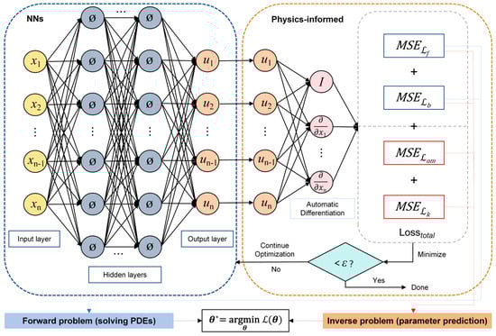
Figure 1. A demonstration of the setup of the proposed MF-rPINN.

3. Problem Setup

3.1. Second-Order Displacement Function

The safety and sustainability of prestressed concrete bridges can be improved with accurate prestress loss prediction [60,61]. Considerable loss of the prestress force may imply damages hidden in the bridge. Recently, such as impedance-based methods [62], elasto-magnetic methods [63], acoustoelastic methods [64], and strain-based methods [65] have been extensively investigated for prestress monitoring. However, embedding multiple sensor technologies into prestressed concrete bridges that have been in service for many years to measure prestress presents a significant challenge. Despite active studies in technologies related to smart materials-based structural health monitoring, such as the piezoelectric active sensing method [66], piezoelectric ceramic transducers [67], and others, they are only able to measure a limited range of prestress. In other words, current mainstream measurement methods primarily focus on detecting the ends of prestressed tendon or deploying sensors during the construction phase. Interested readers can refer to [68,69,70,71] for a comprehensive review of these details. Applying mainstream methods to these structures is challenging, as they were constructed during periods with relatively less advanced monitoring technologies.

We propose a novel approach, which, from the perspective of inverse problem-solving governed by beam-column equations [72], utilizes readily available displacement responses in actual operations to predict prestress force inversely.

As the classic example of the use of the beam-column equations, let us consider a beam on two simple supports (Figure 2) and carrying a single lateral load Q, which focuses on a simply supported prestressed member of length L. The end constraints of a prismatic concrete beam are often known, as are those of the prestressed beam of a bridge deck. The cross-sectional second moment of area I and the length L can be measured in actual scene or obtained from corresponding project drawings. The beam is first subjected to an eccentric prestress force N with respect to the centroid of the cross section and subsequently to a vertical load Q at the midspan. Both the deflection w and w^s at the given instance is represented. The prestress force N and the elastic modulus E of concrete is assumed to be unknown parameters.

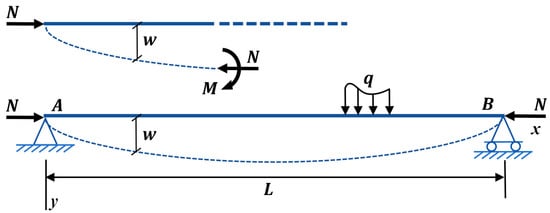
Figure 2. A reference model of the beam-column with a concentrated lateral load.

The corresponding bending moments in the left and right portions of the beam are, respectively, expressed as follows:

$$EI{\displaystyle \frac{d^{2}w}{d{x}^2}}=M\left(x\right)-Nw,$$

(8)

where

$$\begin{gathered} M\left(x\right)=Qx/2 \hspace{1em}\hspace{1em}\hspace{1em}\hspace{1em}\mathrm{for} 0\le x\le L/2, \\ M\left(x\right)=Q\left(L-x\right)/2 \hspace{1em}\hspace{1em}\mathrm{for} L/2\le x\le L. \end{gathered}$$

Since the defection and bending moments are zero at the ends of the bar, the boundary conditions of simply supported beam are defined as

$$w\left(x\right)=0 \mathrm{and} M\left(x\right)=0\hspace{1em}\hspace{1em}\mathrm{at} x=0 \mathrm{and} x=L,$$

(9)

We then consider a second-order effect displacement w^s(x), which exhibits a prior relation by Timoshenko [72] as follows:

$$\begin{gathered} w^s\left(x\right)={\displaystyle \frac{m}{2\sqrt{n^3}}}\left[{\displaystyle \frac{1}{\cos \left(\sqrt{n}/2\right)}}\sin \left(\sqrt{n}{\displaystyle \frac{x}{L}}\right)-\sqrt{n}{\displaystyle \frac{x}{L}}\right]\hspace{1em}\hspace{1em}\hspace{1em}\hspace{1em}\mathrm{for} 0\le x\le L/2, \\ {w}^s\left(x\right)={\displaystyle \frac{m}{2\sqrt{n^3}}}\left[{\displaystyle \frac{1}{\cos \left(\sqrt{n}/2\right)}}\sin \left(\sqrt{n}{\displaystyle \frac{L-x}{L}}\right)-\sqrt{n}{\displaystyle \frac{L-x}{L}}\right]\hspace{1em}\mathrm{for} L/2\le x\le L. \end{gathered}$$

(10)

where n = NL²/EI is the nondimensional axial force, and m = FL³/EI is the load parameter with a length dimension.

More directly, it can be observed that over the prescribed domain, the second-order displacement function is strictly non-negative, which acts as a physically intuitive and strong constraint on the governing differential equation.

In contrast, in the differential equation formulation, expressed as Equation (8), the parameters N or E are not inherently restricted to be non-negative. This may lead to solutions corresponding to negative axial force or modulus, effectively transforming the structural behavior into that of a tension–bending beam, which clearly violates physical intuition.

3.2. Surrogate Model Instantiation Based on MF-rPINN

Based on the Euler–Bernoulli beam theory, Bonopera [73] estimated the prestress force by using one or a set of static displacements measured along the member axis, as shown in Figure 3. However, the implementation of this procedure required information regarding the bending stiffness of the beam. The deflected shape of a post-tensioned concrete beam, subjected to an additional vertical load, was measured in a short term in several laboratory experiments. Specifically, upon positioning the beam on the supports, all geometric dimensions were confirmed to be within a tolerance of 0.01 mm, utilizing precision measurement instruments including a laser rangefinder and calipers. The elastic modulus of the concrete was quantitatively assessed through compression tests conducted after a 28-day curing period and daily during Non-Destructive Testing method simulations in the laboratory. The displacement measurements at seven distinct points, denoted as v₁–v₇, represent the HF data. The physical quantities employed for computations are I, Q, and L, while E and P are utilized for validation purposes.

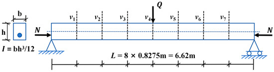
Figure 3. A test layout with locations of the instrumented sections of the sensors (values in meters).

Here, the experimental data of interest have been meticulously compiled (Table 1). For an extensive account and detailed particulars pertaining to the post-tensioned concrete beam specimen and test layout, the readers can refer to [73].

Table 1. Experimental data for the beam-column equations.

Test	Day of Concrete Curing	E (MPa)	N (kN)	Q (kN)	v1 (mm)	v2 (mm)	v3 (mm)	v4 (mm)	v5 (mm)	v6 (mm)	v7 (mm)
1	426th	34,870	620	20.2	1.45	1.95	2.62	2.84	—	1.93	1.02
2	426th	34,870	620	22.6	1.59	2.20	2.95	3.20	—	2.17	1.15
3	426th	34,870	617	25.0	1.42	2.32	3.12	3.43	3.03	2.27	1.22
4	427th	37,618	724	20.1	1.19	1.78	2.39	2.59	2.33	1.73	0.94
5	427th	37,618	721	22.6	1.31	2.00	2.67	2.92	2.60	1.94	1.05
6	427th	37,618	721	25.1	1.46	2.22	2.97	3.23	2.90	2.16	1.17
7	433rd	38,791	820	20.2	1.20	1.75	2.33	2.54	2.29	1.71	0.92
8	433rd	38,791	820	22.9	1.33	1.98	2.65	2.88	2.60	1.94	1.04
9	433rd	38,791	820	25.1	1.42	2.17	2.91	3.17	2.86	2.14	1.15

The overall framework of the proposed MF-rPINN for the forward and inverse analysis of engineering structures is presented in Algorithm 1, which simultaneously demonstrates the process of instantiation for the experiment example.

Algorithm 1. MF-rPINN for the forward and inverse analysis of beam-column structures

1 Determine a task-based loading scenario (the beam-column equations in this paper) for structures to be analyzed at the offline stage. ►Equation (8)

2 Determine the variables (x and w), unknown parameters (E and N), and known parameters (I, Q, and L) in the task. ($MS{E}_{L_f}$) ►Equation (8)

3 Build the corresponding boundary conditions $\mathcal{B}\left(u,x\right)=0$. ($MS{E}_{L_b}$) ►Equation (9)

4 Construct a task-based prior relation (a second-order effect displacement ws in this paper) for instantiating the general form of the relation function k(x; p). ($MS{E}_{L_k}$)

►Equation (10)

5 Generate the coordinates of sampling points Cf, Cb, and Ck.

6 Construct a noisy gappy data set of observational measurements points Com from the actual engineering or laboratory.  ($MS{E}_{L_{om}}$) ►Equation (4)

7 Construct a set of collocation points Ck. ($MS{E}_{L_k}$) ►Equation (6)

8 Build a deep neural networks, and determine the width, depth, activation function, initialization strategy.

9 Determine the learning rate (lr), which is key for feature acquisition; determine the weights (wf, wb, wom, and wk), which are associated with each loss term dictate the preferences during the feature learning process.

10 Minimize the loss function to compute the optimal parameter θ*. ►Equation (7)

The employed neural network architectures consist of three hidden layers, each containing 40 neurons and utilizing the hyperbolic tangent (tanh) activation function. Observational measurements are derived from synthetic laboratory data reported in ref. [73]. Model implementation and training were carried out using TensorFlow [74] on Google Colab, leveraging an NVIDIA A100 GPU. Parameter optimization was performed with the Adam algorithm [75]. The specific hyperparameter configurations and task-dependent settings are summarized in Table 2.

Table 2. Hyperparameters and task-based parameters setting for this example.

Parameters			Value
Hyperparameters
neural networks		Cf	20,000
		Cb	100
		Ck	20,000
		Com	Test 1	Test 2	Test 3
			6	6	7
			Test 4	Test 5	Test 6
			7	7	7
			Test 7	Test 8	Test 9
			7	7	7
		wf	0.000001
		wb	100
		wom	10,000
		wk	0.000001
		lr	0.00001
Task-based parameters
variables	is assumed to be known	I	1.3333333333 × 10−3 m4
		Q	Test 1	Test 2	Test 3
			20.2 kN	22.6 kN	25.0 kN
			Test 4	Test 5	Test 6
			20.1 kN	22.6 kN	25.1 kN
			Test 7	Test 8	Test 9
			20.2 kN	22.9 kN	25.1 kN
		L	6.62 m
	is assumed to be known/unknown parameters for forward/inverse problems	N	Test 1	Test 2	Test 3
			620 kN	620 kN	617 kN
			Test 4	Test 5	Test 6
			724 kN	721 kN	721 kN
			Test 7	Test 8	Test 9
			820 kN	820 kN	820 kN
		E	Test 1, 2, 3	Test 4, 5, 6	Test 7, 8, 9
			34,870 MPa	37,618 MPa	38,791 MPa

4. Method Validation and Evaluation

In this section, we validate the rationality of MF-rPINN from two perspectives: the prediction of forward and inverse problems. We demonstrate the effectiveness of MF-rPINN in predicting continuous displacement fields, prestress force, and elastic modulus, based on MF-rPINN that incorporate MF data and a second-order effect displacement function. Furthermore, an evaluation of the MF-rPINN was conducted by comparing outcomes derived from two established methodologies: the theory of elastic stability and PINN.

4.1. Forward Problem: Continuous Displacement Field

Here, the theory of elastic stability necessitates the assumption that the parameters E and N are known, whereas PINN and MF-PINN operate under the premise that E and N are unknown parameters. Three different methods, i.e., Timoshenko, PINN, and MF-rPINN are implemented for comparative analysis against nine sets of experimental results. Figure 4 shows the continuous displacement field of the three methods after computation or training. We observed that, due to the nearly identical outcomes produced by PINN and MF-rPINN in the prediction of forward problems, the results of PINN are delineated separately in Figure 4a,c,e for the purpose of differentiation and comparison.

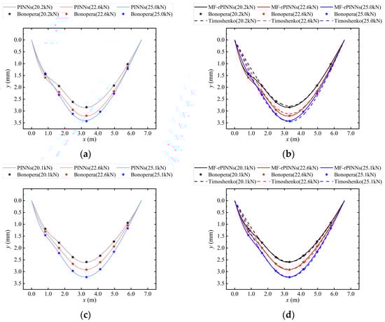
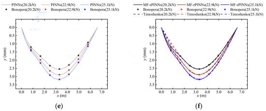
Figure 4. The prediction of w and the observational measurements from nine sets of graded loading tests. The light lines represent the results obtained from PINN; the dark lines represent the results obtained from MF-rPINN; the dashed lines correspond to the approximations by Timoshenko [72]; the star points represent the Bonopera’s experimental results [73]; different colors are utilized to denote various test conditions. (a,b) correspond to Test 1, 2, and 3; (c,d) to Test 4, 5, and 6; (e,f) to Test 7, 8, and 9. (a,c,e) represent the predictions from PINN under different test conditions; (b,d,f) represent the predictions from MF-rPINN, and the approximate solutions by Timoshenko under different test conditions.

We have found that all nine sets of Bonopera’s experimental results exhibit characteristics that deviate from physical intuition to varying degrees, particularly evident in Figure 4a. Specifically, the values of v₁–v₂ in Test 1, 2, and 3 did not manifest the expected physical characteristics during the incremental loading process: a progressive increase (Test 1 < Test 2 < Test 3) was anticipated, rather than the observed sequence of Test 1 ≈ Test 3 < Test 2. Furthermore, these observational measurements do not satisfy the physical symmetry with respect to the midspan cross-section. Although Timoshenko method yields results that comply with the laws of physics, as shown in Figure 4b,d,f, this outcome not only presupposes both E and P are known, but also fails to seamlessly incorporate these observational measurements. PINN and MF-rPINN are capable of perceiving and incorporating these observational measurements, implying that predictions consistent with physical laws can be made for other unobserved points without the need for direct measurement, such as for a continuous displacement field in this paper.

It is emphasized that the experimental data employed in this paper are not treated as noise-free ground truth, but rather as realistic engineering measurements subject to uncertainty arising from sensor placement, measurement noise, and experimental asymmetry. In inverse PINN formulations, such uncertainties may be amplified, leading to physically implausible parameter estimates despite low data residuals.

By integrating task-based prior relations, MF-rPINN mitigates this effect by balancing observational data with physically motivated constraints. This balance reduces sensitivity to local measurement inconsistencies while preserving the ability to fit global structural responses.

4.2. Inverse Problem: Solution of Unknown Prestress Force and Elastic Modulus

Here, since the Timoshenko method is difficult to complete the inverse problem, we consider comparing the prediction ability of PINN and MF-rPINN in all nine sets of Bonopera’s experimental results, as shown in Figure 5. In this section, we consider both E and N are unknown parameters.

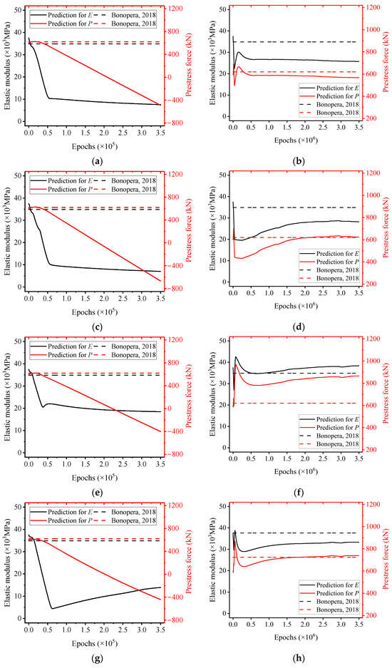
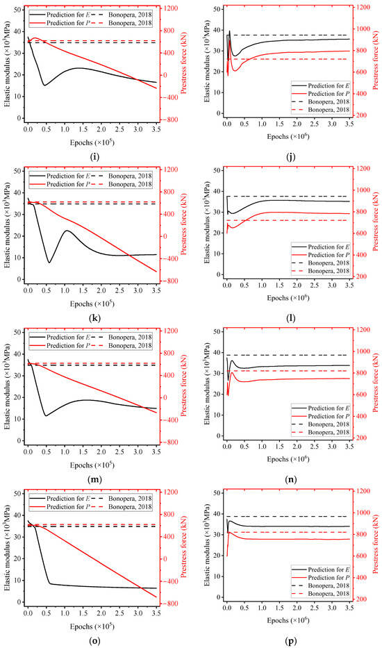
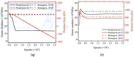
Figure 5. Comparison of the predictions for E and N across nine sets of graded loading tests between PINN and MF-rPINN. The black lines represent elastic modulus; the red lines represent prestress force; the dashed lines represent Bonopera’s experimental results [73]. Each independent test (Test 1~9) correspond to (a,b), (c,d), (e,f), (g,h), (i,j), (k,l), (m,n), (o,p), (q,r). (a,c,e,g,i,k,m,o,q) represent the predictions from PINN. (b,d,f,h,j,l,n,p,r) represent the predictions from MF-rPINN.

Figure 5a,c,e,g,i,k,m,o,q collectively suggest that PINN are incapable of simultaneously predicting parameters E and N with accuracy. This deficiency is mainly manifested in two aspects: with the increase in training epochs, the predicted prestress force rapidly decreases and converges to a negative value (i.e., N ≈ −700 kN in Test 2, N ≈ −300 kN in Test 6, and N ≈ −610 kN in Test 9), a result that not only contravenes physical intuition but also contradicts the initial conditions of the experiments. On the other hand, the corresponding elastic modulus also decreases with the number of training epochs and converges to an erroneous value (i.e., E ≈ 8 Gpa in Test 2, E ≈ 9 Gpa in Test 8, and E ≈ 15 Gpa in Test 9). Typically, concrete with a strength of approximately 10 Gpa is utilized solely in applications such as subgrade fill or landscape design.

The occurrence of nonphysical inverse solutions, such as negative prestress forces observed in classical PINN results, is not solely attributable to numerical optimization difficulties. Rather, it reflects the non-identifiability and non-closure of the inverse problem, where multiple parameter combinations can reproduce similar displacement fields while violating physical admissibility. MF-rPINN addresses this issue by restricting the feasible solution space through task-based priors, thereby transforming an ill-posed inverse problem into a physically identifiable one. This distinction highlights that the improvement achieved by MF-rPINN arises from enhanced problem formulation rather than optimization alone.

This is primarily due to the difficulty in acquiring HF observational data, which is sparse and significantly noisy. Specifically, the small number of observational measurements is disproportionately low compared to the number of collocation points in the spatiotemporal domain, and although we can align the PINN predictions closely with these measurements for forward problems, there remain multiple sets of parameter predictions for inverse problems that satisfy the predictive solutions of forward problems mathematically. Furthermore, the noise in observational measurements sometimes exhibits noncompliance with physical symmetries and conservation laws, leading to significant deviation of the PINN gradients from the characteristics of the PDE, thus steering the results towards increased errors. Therefore, relying solely on differential equations and a limited set of HF data is insufficient to address inverse problems in actual engineering and experimental science tasks. It is evident that while PINN are adept at identifying the optimal output from a mathematical perspective when addressing forward problems, they begin to falter when confronted with inverse problems that incorporate noise. Consequently, it becomes imperative to incorporate additional prior information, specifically an enhanced relation function that is guided by the task at hand.

Correspondingly, we observe that MF-rPINN exhibits superior predictive performance compared to PINN in integrating MF data, as illustrated in Figure 5b,d,f,h,j,l,n,p,r. Guided by Equations (4) and (6), the prediction results are rendered more consistent with engineering experience. With the increase in training epochs, the predicted prestress force converges to a more reasonable value (i.e., N ≈ 620 kN in Test 2, N ≈ 780 kN in Test 6, and N ≈ 780 kN in Test 9), a result that matches the initial conditions of the test is obtained at the expense of more training time. The corresponding elastic modulus also converges to a reasonable value (i.e., E ≈ 28 Gpa in Test 2, E ≈ 34 Gpa in Test 8, and E ≈ 34 Gpa in Test 9).

MF-rPINN demonstrates commendable performance capabilities, thanks to the enhanced physical relations, when experimental data exhibit significant noise. As shown in Figure 5b,f, it is precisely these sets of experimental data that exhibit characteristics counter to physical intuition, a feature also discussed in Section 4.1. Although the results of MF-rPINN appear to deviate slightly from the initial conditions, this error can be mitigated through multiple sets of experimental measurements.

To further evaluate the capability of MF-rPINN in addressing inverse problems, an error analysis was conducted, as shown in Table 3. The performance of MF-rPINN is evaluated solely based on Bonopera’s optimal experimental results, due to the inability of PINN to yield satisfactory results and Timoshenko’s failure to integrate MF data.

Table 3. The prediction errors (Δ_E and Δ_P) for nine sets of graded loading tests with MF-rPINN.

Test	Elastic Modulus			Prestress Force
	Parameter E (MPa)	Bonopera ΔE (%)	MF-rPINN ΔE(%)	Parameter P (kN)	Bonopera ΔP(%)	MF-rPINN ΔP(%)
1	34,870	-	−26.23	620	−26.60	−8.39
2	34,870		−19.13	620	−15.20	0.65
3	34,870		10.12	617	−17.20	39.84
4	37,618		−11.68	724	−2.20	2.07
5	37,618		−5.01	721	3.20	10.26
6	37,618		−6.49	721	−4.80	8.46
7	38,791		−12.80	820	−1.10	−8.66
8	38,791		−12.22	820	−1.10	−7.80
9	38,791		−9.32	820	−1.30	−4.51
Method of acquisition	compression tests	compression tests	prediction	hydraulic oil jack	prediction	prediction
Known /unknown	-	known	unknown	-	unknown	unknown

Table 3 shows that the largest errors occurred in Test 1 (Δ_E ≈ 6% and Δ_P ≈ 8%) and Test 3 (Δ_E ≈ 10% and Δ_P ≈ 40%). The remaining experimental results are more reasonable, with the relative generally remaining below 10%. Therefore, more reasonable predictive results can be obtained using MF-rPINN by conducting multiple parallel experiments. It is significant to note that MF-rPINN not only accomplished the prediction of prestress force with accuracy levels comparable to those observed in Bonopera’s experiment, where average errors, Δ_P,aver, were approximately 10% and 8% respectively, but also facilitated the prediction of the elastic modulus. This indicates that outcomes with an average error Δ_E, aver of approximately 12% are achievable without the necessity of conducting compression tests. These observations provide new insights for the reverse adjustment of elastic modulus measurements obtained via compression tests.

Finally, we summarize the objectives achieved by MF-rPINN in this task: by conducting graded loading tests and obtaining a sparse set of observational measurements, it is feasible to (1) reasonably predict the continuous displacement field, (2) concurrently predict the prestress force and elastic modulus, and (3) evaluate the error in the experimental data.

5. Discussion

Next, we focus our discussion on the impact of hyperparameter selection within neural networks on the MF-rPINN algorithm. In this section, we further elucidate how this algorithm identifies the optimal hyperparameters settings for physics feature acquisition and preference during the learning process. In addressing forward PDE problems, MF-rPINN have demonstrated capabilities comparable to those of PINN, which are now unable to concurrently predict N and P. Consequently, our discussion focus on specific hyperparameters for MF-rPINN tailored to solving inverse problems. In this section, we consider experimental scenarios where Q remains constant while E and P change simultaneously (Test 1, Test 4, and Test 7).

5.1. Learning Rate

Three orders of magnitude for the learning rate (lr = 1 × 10⁻³, 1 × 10⁻⁵, and 1 × 10⁻⁷) are investigated, as shown in Figure 6, with other parameters fixed according to Table 2. Results from three experimental groups indicate that MF-rPINN can converge to satisfactory predictions of both elastic modulus E and prestress force N across all tested learning rates. However, excessively large learning rates lead to overshooting behavior and increased runtime, consistent with observations in [76,77]. Considering both stability and efficiency, lr = 1 × 10⁻⁵ is adopted in this paper.

Figure 6. Simultaneous predictions for E and N with learning rates of different orders of magnitude. The different colors represent learning rates of varying orders of magnitude. The lighter lines represent the elastic modulus; the darker lines represent the prestress force; the dashed lines represent Bonopera’s experimental results [73]. Each independent test (Test 1, 4, and 7) correspond to (a–c).

5.2. Weights

After fixing the learning rate, we examine the influence of loss weights associated with observational measurements (w_om) and the enhanced relation function (w_k), as summarized in Table 4. Figure 7 and Figure 8 show that variations in w_k and w_om significantly affect the simultaneous identification of E and N. In general, increasing w_om strengthens the influence of observational data, while w_k controls the enforcement strength of the second-order displacement relation. The results suggest that the effectiveness of MF-rPINN depends on a balanced configuration of these weights rather than their absolute magnitudes. Based on the observed stability and accuracy, Setting 3 is selected as the preferred configuration in this paper.

Table 4. Weight values for settings.

	Value
	Setting 1	Setting 2	Setting 3	Setting 4	Setting 5
wom	1 × 104	1 × 104	1 × 104	1 × 102	1 × 100
wk	1 × 10−2	1 × 10−4	1 × 10−6	1 × 10−6	1 × 10−6

Figure 7. Simultaneous predictions for E and N with different w_k while w_om = 1 × 10⁴. The different colors represent varying settings; the solid lines represent elastic modulus; the dotted lines represent prestress force; the dashed lines represent Bonopera’s experimental results [73]. Each independent test (Test 1, 4, and 7) correspond to (a–c).

Figure 8. Simultaneous predictions for E and N with different w_om while w_k = 1 × 10⁻⁶. The different colors represent varying settings; the solid lines represent elastic modulus; the dotted lines represent prestress force; the dashed lines represent Bonopera’s experimental results [73]. Each independent test (Test 1, 4, and 7) correspond to (a–c).

5.3. Neurons and Layer Size

We then discuss the impacts of six different network architectures on the performance of MF-rPINN, as shown in Table 5. The neural network architecture is intentionally fixed to isolate the effect of the proposed MF-rPINN formulation.

Table 5. Network architecture setup.

	Value
	Setting 1	Setting 2	Setting 3	Setting 4	Setting 5
Layer size	3	3	3	4	4
Neurons	20	30	40	20	30

As shown in Figure 9, the predicted values of E and N are relatively insensitive to architectural variations, indicating that MF-rPINN is robust with respect to network size. However, runtime differences are non-negligible, as illustrated in Figure 10. Deeper or wider networks generally incur higher computational costs without noticeable accuracy gains. Considering efficiency and convergence behavior, a network with three hidden layers and 40 neurons per layer is adopted.

Figure 9. Simultaneous predictions for E and N with different network architectures. The different colors represent varying settings; the solid lines represent elastic modulus; the lighter lines represent prestress force; the darker lines represent Bonopera’s experimental results [73]. Each independent test (Test 1, 4, and 7) correspond to (a–f).

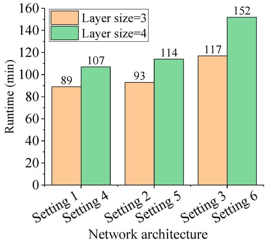
Figure 10. Runtimes of different network architectures. The orange color represent the runtime when the layer size is 3; the green color represent the runtime when the layer size is 4.

5.4. Observational Measurements and Collocation Points

The ratio r_oc between the number of observational measurements and collocation points plays a critical role in inverse performance. As shown in Table 6 and Figure 11, larger ratios correspond to less stable and less accurate predictions, particularly when observational measurements are sparse and noisy. When r_oc ≤ 6/200, the predictions of E and N become stable across all experimental groups. This observation highlights the sensitivity of inverse PINN-based methods to noisy observational data. The increased runtime associated with larger numbers of collocation points is shown in Figure 12. These results further motivate the introduction of additional physics-based loss terms in Equations (4) and (6) to regularize inverse identification under sparse and noisy measurements.

Table 6. Observational measurements and collocation points setup.

	Test 1	Test 4	Test 7
	Number
Observational measurements	6	7	7
Collocation points	20	20	20
	200	200	200
	2000	2000	2000
	20,000	20,000	20,000
roc	6/20	7/20	7/20
	6/200	7/200	7/200
	6/2000	7/2000	7/2000
	6/20,000	7/20,000	7/20,000

Figure 11. Simultaneous predictions for E and N with different ratios. The different colors represent varying ratios r_oc; the solid lines represent elastic modulus; the dotted lines represent prestress force; the dashed lines represent Bonopera’s experimental results [73]. Each independent test (Test 1, 4, and 7) correspond to (a–c).

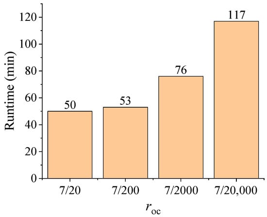
Figure 12. Runtime of different ratios r_oc.

Across Section 5.1, Section 5.2, Section 5.3 and Section 5.4, MF-rPINN consistently demonstrates robust convergence with respect to learning rate, network architecture, and collocation density, provided that loss weights are properly balanced. While prediction accuracy is relatively insensitive to architectural choices, inappropriate learning rates, loss-weight configurations, or excessively high ratios of observational measurements to collocation points can degrade convergence efficiency or stability. These findings suggest that MF-rPINN possesses strong robustness to hyperparameter variations, with performance primarily governed by the interplay between data fidelity and physics-based regularization.

6. Conclusions

This study proposed a multi-fidelity data and prior-enhanced physics-informed neural network (MF-rPINN) framework to address inverse identification problems governed by partial differential equations using sparse and noisy experimental data. By integrating heterogeneous multi-fidelity data with task-oriented prior relational constraints, MF-rPINN extends the classical PINN formulation and guides the learning process toward physically admissible parameter solutions. The theoretical foundation of the proposed method highlights the critical roles of data fidelity and prior information in shaping the network architecture and loss formulation for inverse problems.

The effectiveness of MF-rPINN was validated through beam-column problems involving both forward and inverse tasks. Compared with classical PINN, MF-rPINN demonstrated superior robustness in handling noisy and incomplete observations, particularly in inverse identification of prestress force and elastic modulus. Quantitative results show that the minimum relative errors of the elastic modulus reach −6.49% and −9.32% under different and identical loading conditions, respectively, while the minimum relative errors of the prestress force are 0.65% and 4.51%. These improvements are attributed to the combined regularization effects of governing physical laws and the second-order displacement prior embedded in the loss function.

From an engineering perspective, MF-rPINN enables the simultaneous prediction of continuous displacement fields and inverse identification of key structural parameters using operational displacement responses. This capability is particularly relevant for the assessment of prestressed concrete bridges that have been in long-term service, where direct measurement of prestress force is difficult or infeasible. By balancing physical relations among parameters and accommodating flexible data scales under different loading scenarios, MF-rPINN shows strong potential as a surrogate modeling tool for practical engineering applications.

Future work will focus on the following: (1) extending the applicability of MF-rPINN to address a broader range of complex multi-physics problems; (2) the intentional fixing of the neural network architecture to isolate the effect of the proposed MF-rPINN formulation, with alternative architectures potentially further improving convergence or robustness; (3) developing more principled and adaptive loss-weighting strategies to further enhance the robustness and general applicability of MF-rPINN, beyond the sensitivity-based weighting approach adopted in this paper; (4) extending the validation of MF-rPINN to unseen load cases and boundary conditions is identified as an important direction for future work to rigorously assess its surrogate modeling capability.

References

- Meng, C.; Seo, S.; Cao, D.; Griesemer, S.; Liu, Y. When physics meets machine learning: A survey of physics-informed machine learning. arXiv 2022, arXiv:2203.16797. [Google Scholar] [CrossRef]
- Xing, Y.; Gen, L.I.; Yuan, Y. A review of the analytical solution methods for the eigenvalue problems of rectangular plates. Int. J. Mech. Sci. 2022, 221, 107171. [Google Scholar] [CrossRef]
- Chen, Y.; Yu, B.; Lu, W.; Wang, B.; Sun, D.; Jiao, K.; Tao, W. Review on numerical simulation of boiling heat transfer from atomistic to mesoscopic and macroscopic scales. Int. J. Heat Mass Transf. 2024, 225, 125396. [Google Scholar] [CrossRef]
- Karniadakis, G.E.; Kevrekidis, I.G.; Lu, L.; Perdikaris, P.; Wang, S.; Yang, L. Physics-informed machine learning. Nat. Rev. Phys. 2021, 3, 422–440. [Google Scholar] [CrossRef]
- Bingham, D.; Butler, T.; Estep, D. Inverse Problems for Physics-Based Process Models. Annu. Rev. Stat. Its Appl. 2024, 11, 461–482. [Google Scholar] [CrossRef]
- Gallet, A.; Rigby, S.; Tallman, T.N.; Kong, X.; Hajirasouliha, I.; Liew, A.; Liu, D.; Chen, L.; Hauptmann, A.; Smyl, D. Structural engineering from an inverse problems perspective. Proc. R. Soc. A 2022, 478, 20210526. [Google Scholar] [CrossRef]
- Cuomo, S.; Di Cola, V.S.; Giampaolo, F.; Rozza, G.; Raissi, M.; Piccialli, F. Scientific machine learning through physics–informed neural networks: Where we are and what’s next. J. Sci. Comput. 2022, 92, 88. [Google Scholar] [CrossRef]
- Chakraborty, S. Simulation free reliability analysis: A physics-informed deep learning based approach. arXiv 2020, arXiv:2005.01302. [Google Scholar] [CrossRef]
- Darbon, J.; Meng, T. On some neural network architectures that can represent viscosity solutions of certain high dimensional Hamilton–Jacobi partial differential equations. J. Comput. Phys. 2021, 425, 109907. [Google Scholar] [CrossRef]
- Kharazmi, E.; Zhang, Z.; Karniadakis, G.E. hp-VPINN: Variational physics-informed neural networks with domain decomposition. Comput. Methods Appl. Mech. Eng. 2021, 374, 113547. [Google Scholar] [CrossRef]
- Peng, W.Q.; Chen, Y. PT-symmetric PINN for integrable nonlocal equations: Forward and inverse problems. Chaos 2024, 34, 043124. [Google Scholar] [CrossRef]
- Raissi, M.; Perdikaris, P.; Karniadakis, G.E. Physics-informed neural networks: A deep learning framework for solving forward and inverse problems involving nonlinear partial differential equations. J. Comput. Phys. 2019, 378, 686–707. [Google Scholar] [CrossRef]
- Lu, L.; Meng, X.; Mao, Z.; Karniadakis, G.E. DeepXDE: A deep learning library for solving differential equations. SIAM Rev. 2021, 63, 208–228. [Google Scholar] [CrossRef]
- Pang, G.; Lu, L.; Karniadakis, G.E. fPINN: Fractional physics-informed neural networks. SIAM J. Sci. Comput. 2019, 41, A2603–A2626. [Google Scholar] [CrossRef]
- Yang, L.; Zhang, D.; Karniadakis, G.E. Physics-informed generative adversarial networks for stochastic differential equations. SIAM J. Sci. Comput. 2020, 42, A292–A317. [Google Scholar] [CrossRef]
- Fernández-Godino, M.G. Review of multi-fidelity models. arXiv 2016, arXiv:1609.07196. [Google Scholar] [CrossRef]
- Cheung, H.L.; Mirkhalaf, M. A multi-fidelity data-driven model for highly accurate and computationally efficient modeling of short fiber composites. Compos. Sci. Technol. 2024, 246, 110359. [Google Scholar] [CrossRef]
- Conti, P.; Guo, M.; Manzoni, A.; Frangi, A.; Brunton, S.L.; Nathan Kutz, J. Multi-fidelity reduced-order surrogate modelling. Proc. R. Soc. A 2024, 480, 20230655. [Google Scholar] [CrossRef]
- Jansson, N.; Karp, M.; Podobas, A.; Markidis, S.; Schlatter, P. Neko: A modern, portable, and scalable framework for high-fidelity computational fluid dynamics. Comput. Fluids 2024, 275, 106243. [Google Scholar] [CrossRef]
- Kennedy, M.C.; O’Hagan, A. Predicting the output from a complex computer code when fast approximations are available. Biometrika 2000, 87, 1–13. [Google Scholar] [CrossRef]
- Liu, J.; Shi, Y.; Ding, C.; Beer, M. Hybrid uncertainty propagation based on multi-fidelity surrogate model. Comput. Struct. 2024, 293, 107267. [Google Scholar] [CrossRef]
- Feng, D.C.; Chen, S.Z.; Taciroglu, E. Deep learning-enhanced efficient seismic analysis of structures with multi-fidelity modeling strategies. Comput. Methods Appl. Mech. Eng. 2024, 421, 116775. [Google Scholar] [CrossRef]
- Mao, R.; Jiao, J.J.; Luo, X. Quantifying time-variant travel time distribution and internal mixing by multi-fidelity model under nonstationary hydrologic conditions. Adv. Water Resour. 2024, 186, 104662. [Google Scholar] [CrossRef]
- Lu, N.; Li, Y.F.; Mi, J.; Huang, H.Z. AMFGP: An active learning reliability analysis method based on multi-fidelity Gaussian process surrogate model. Reliab. Eng. Syst. Saf. 2024, 246, 110020. [Google Scholar] [CrossRef]
- Fischer, C.C.; Grandhi, R.V.; Beran, P.S. Bayesian low-fidelity correction approach to multi-fidelity aerospace design. In Proceedings of the 58th AIAA/ASCE/AHS/ASC Structures, Structural Dynamics, and Materials Conference, Grapevine, TX, USA, 9–13 January 2017; p. 0133. [Google Scholar] [CrossRef]
- Sharma, A.; Sankar, B.; Haftka, R. Multi-fidelity analysis of corrugated-core sandwich panels for integrated thermal protection systems. In Proceedings of the 50th AIAA/ASME/ASCE/AHS/ASC Structures, Structural Dynamics, and Materials Conference, Palm Springs, CA, USA, 4–7 May 2009; p. 2201. [Google Scholar] [CrossRef]
- Singh, G.; Grandhi, R.V. Mixed-variable optimization strategy employing multifidelity simulation and surrogate models. AIAA J. 2010, 48, 215–223. [Google Scholar] [CrossRef]
- Berthet, S.; Séférian, R.; Bricaud, C.; Chevallier, M.; Voldoire, A.; Ethé, C. Evaluation of an online grid-coarsening algorithm in a global eddy-admitting ocean biogeochemical model. J. Adv. Model. Earth Syst. 2019, 11, 1759–1783. [Google Scholar] [CrossRef]
- Asghari, M.; Fathollahi-Fard, A.M.; Mirzapour Al-E-Hashem, S.M.J.; Dulebenets, M.A. Transformation and linearization techniques in optimization: A state-of-the-art survey. Mathematics 2022, 10, 283. [Google Scholar] [CrossRef]
- Cattaneo, P.; Lenain, R.; Merle, E.; Patricot, C.; Schneider, D. Numerical optimization of a multiphysics calculation scheme based on partial convergence. Ann. Nucl. Energy 2021, 151, 107892. [Google Scholar] [CrossRef]
- Mulmuley, K.D.; Sohoni, M. Geometric complexity theory I: An approach to the P vs. NP and related problems. SIAM J. Comput. 2001, 31, 496–526. [Google Scholar] [CrossRef]
- Towne, A.; Dawson, S.T.M.; Brès, G.A.; Lozano-Durán, A.; Saxton-Fox, T.; Parthasarathy, A.; Jones, A.R.; Biler, H.; Yeh, C.-A.; Patel, H.D.; et al. A database for reduced-complexity modeling of fluid flows. AIAA J. 2023, 61, 2867–2892. [Google Scholar] [CrossRef]
- Aliakbari, M.; Mahmoudi, M.; Vadasz, P.; Arzani, A. Predicting high-fidelity multiphysics data from low-fidelity fluid flow and transport solvers using physics-informed neural networks. Int. J. Heat Fluid Flow 2022, 96, 109002. [Google Scholar] [CrossRef]
- Balachandar, S. Lagrangian and Eulerian drag models that are consistent between Euler-Lagrange and Euler-Euler (two-fluid) approaches for homogeneous systems. Phys. Rev. Fluids 2020, 5, 084302. [Google Scholar] [CrossRef]
- Bahmani, B.; Sun, W. A kd-tree-accelerated hybrid data-driven/model-based approach for poroelasticity problems with multi-fidelity multi-physics data. Comput. Methods Appl. Mech. Eng. 2021, 382, 113868. [Google Scholar] [CrossRef]
- Olleak, A.; Xi, Z. Calibration and validation framework for selective laser melting process based on multi-fidelity models and limited experiment data. J. Mech. Des. 2020, 142, 081701. [Google Scholar] [CrossRef]
- Meng, X.; Karniadakis, G.E. A composite neural network that learns from multi-fidelity data: Application to function approximation and inverse PDE problems. J. Comput. Phys. 2020, 401, 109020. [Google Scholar] [CrossRef]
- Mao, Z.; Jagtap, A.D.; Karniadakis, G.E. Physics-informed neural networks for high-speed flows. Comput. Methods Appl. Mech. Eng. 2020, 360, 112789. [Google Scholar] [CrossRef]
- Rao, C.; Sun, H.; Liu, Y. Physics-informed deep learning for incompressible laminar flows. Theor. Appl. Mech. Lett. 2020, 10, 207–212. [Google Scholar] [CrossRef]
- Zhang, Y.; Zhang, R.F.; Yuen, K.V. Neural network-based analytical solver for Fokker–Planck equation. Eng. Appl. Artif. Intell. 2023, 125, 106721. [Google Scholar] [CrossRef]
- Chen, X.; Yang, L.; Duan, J.; Karniadakis, G.E. Solving Inverse Stochastic Problems from Discrete Particle Observations Using the Fokker--Planck Equation and Physics-Informed Neural Networks. SIAM J. Sci. Comput. 2021, 43, B811–B830. [Google Scholar] [CrossRef]
- Goswami, S.; Anitescu, C.; Chakraborty, S.; Rabczuk, T. Transfer learning enhanced physics informed neural network for phase-field modeling of fracture. Theor. Appl. Fract. Mech. 2020, 106, 102447. [Google Scholar] [CrossRef]
- Liu, Y.; Liu, W.; Yan, X.; Guo, S.; Zhang, C.A. Adaptive transfer learning for PINN. J. Comput. Phys. 2023, 490, 112291. [Google Scholar] [CrossRef]
- Chen, X.; Gong, C.; Wan, Q.; Deng, L.; Wan, Y.; Liu, Y.; Chen, B.; Liu, J. Transfer learning for deep neural network-based partial differential equations solving. Adv. Aerodyn. 2021, 3, 36. [Google Scholar] [CrossRef]
- Tang, H.; Liao, Y.; Yang, H.; Xie, L. A transfer learning-physics informed neural network (TL-PINN) for vortex-induced vibration. Ocean Eng. 2022, 266, 113101. [Google Scholar] [CrossRef]
- Lin, S.; Chen, Y. Gradient-enhanced physics-informed neural networks based on transfer learning for inverse problems of the variable coefficient differential equations. Phys. D Nonlinear Phenom. 2024, 459, 134023. [Google Scholar] [CrossRef]
- Xu, C.; Cao, B.T.; Yuan, Y.; Meschke, G. Transfer learning based physics-informed neural networks for solving inverse problems in engineering structures under different loading scenarios. Comput. Methods Appl. Mech. Eng. 2023, 405, 115852. [Google Scholar] [CrossRef]
- Wu, S.; Lu, B. INN: Interfaced neural networks as an accessible meshless approach for solving interface PDE problems. J. Comput. Phys. 2022, 470, 111588. [Google Scholar] [CrossRef]
- Moseley, B.; Markham, A.; Nissen-Meyer, T. Finite Basis Physics-Informed Neural Networks (FBPINN): A scalable domain decomposition approach for solving differential equations. Adv. Comput. Math. 2023, 49, 62. [Google Scholar] [CrossRef]
- Jagtap, A.D.; Karniadakis, G.E. Extended physics-informed neural networks (XPINN): A generalized space-time domain decomposition based deep learning framework for nonlinear partial differential equations. Commun. Comput. Phys. 2020, 28, 2002–2041. [Google Scholar] [CrossRef]
- Meng, X.; Li, Z.; Zhang, D.; Karniadakis, G.E. PPINN: Parareal physics-informed neural network for time-dependent PDEs. Comput. Methods Appl. Mech. Eng. 2020, 370, 113250. [Google Scholar] [CrossRef]
- Costabal, F.S.; Pezzuto, S.; Perdikaris, P. Δ-PINN: Physics-informed neural networks on complex geometries. arXiv 2022, arXiv:2209.03984. [Google Scholar] [CrossRef]
- Hennigh, O.; Narasimhan, S.; Nabian, M.A.; Subramaniam, A.; Tangsali, K.; Fang, Z.; Rietmann, M.; Byeon, W.; Choudhry, S. NVIDIA SimNet™: An AI-accelerated multi-physics simulation framework. In Proceedings of the International Conference on Computational Science, Krakow, Poland, 16–18 June 2021; Springer International Publishing: Cham, Switzerland; pp. 447–461. [Google Scholar] [CrossRef]
- Zou, Z.; Meng, X.; Psaros, A.F.; Karniadakis, G.E. NeuralUQ: A comprehensive library for uncertainty quantification in neural differential equations and operators. arXiv 2022, arXiv:2208.11866. [Google Scholar] [CrossRef]
- Bono, F.M.; Radicioni, L.; Cinquemani, S. A comparison between regular and physics-informed neural networks based on a numerical multibody model: A test case for the synthesis of mechanisms. In Proceedings of the NDE 4.0, Predictive Maintenance, Communication, and Energy Systems: The Digital Transformation of NDE, Long Beach, CA, USA, 12–17 March 2023; SPIE: Bellingham, DC, USA, 2023; Volume 12489, pp. 101–109. [Google Scholar] [CrossRef]
- Wang, S. Evaluating cross-building transferability of attention-based automated fault detection and diagnosis for air handling units: Auditorium and hospital case study. Build. Environ. 2025, 287, 113889. [Google Scholar] [CrossRef]
- Wang, S. Automated Fault Diagnosis Detection of Air Handling Units Using Real Operational Labelled Data Using Transformer-based Methods at 24-hour operation Hospital. Build. Environ. 2025, 282, 113257. [Google Scholar] [CrossRef]
- Zhang, X.S. Neural Networks in Optimization; Springer Science & Business Media: Dordrecht, The Netherlands, 2013; Volume 46. [Google Scholar] [CrossRef]
- Abdolrasol, M.G.M.; Hussain, S.M.S.; Ustun, T.S.; Sarker, M.R.; Hannan, M.A.; Mohamed, R.; Ali, J.A.; Mekhilef, S.; Milad, A. Artificial neural networks based optimization techniques: A review. Electronics 2021, 10, 2689. [Google Scholar] [CrossRef]
- Sung, Y.C.; Lin, T.K.; Chiu, Y.T.; Chang, K.C.; Chen, K.L.; Chang, C.C. A bridge safety monitoring system for prestressed composite box-girder bridges with corrugated steel webs based on in-situ loading experiments and a long-term monitoring database. Eng. Struct. 2016, 126, 571–585. [Google Scholar] [CrossRef]
- Noble, D.; Nogal, M.; O’Connor, A.; Pakrashi, V. The effect of prestress force magnitude and eccentricity on the natural bending frequencies of uncracked prestressed concrete beams. J. Sound Vib. 2016, 365, 22–44. [Google Scholar] [CrossRef]
- Huynh, T.C.; Kim, J.T. RBFN-based temperature compensation method for impedance monitoring in prestressed tendon anchorage. Struct. Control Health Monit. 2018, 25, e2173. [Google Scholar] [CrossRef]
- Zhang, S.; Zhang, H.; Zhou, J.; Liu, H.; Ma, H.; Liao, L. Alternating prestress monitoring of steel strands based on the magnetoelastic inductance method. Measurement 2022, 194, 111024. [Google Scholar] [CrossRef]
- Pirskawetz, S.M.; Schmidt, S. Detection of wire breaks in prestressed concrete bridges by Acoustic Emission analysis. Dev. Built Environ. 2023, 14, 100151. [Google Scholar] [CrossRef]
- Ye, C.; Butler, L.J.; Elshafie, M.Z.; Middleton, C.R. Evaluating prestress losses in a prestressed concrete girder railway bridge using distributed and discrete fibre optic sensors. Constr. Build. Mater. 2020, 247, 118518. [Google Scholar] [CrossRef]
- Jiang, J.; Ho, S.C.M.; Tippitt, T.; Chen, Z.; Song, G. Feasibility study of a touch-enabled active sensing approach to inspecting subsea bolted connections using piezoceramic transducers. Smart Mater. Struct. 2020, 29, 085038. [Google Scholar] [CrossRef]
- Kong, Q.; Fan, S.; Mo, Y.L.; Song, G. A novel embeddable spherical smart aggregate for structural health monitoring: Part II. Numerical and experimental verifications. Smart Mater. Struct. 2017, 26, 095051. [Google Scholar] [CrossRef]
- Mo, D.; Zhang, L.; Wang, L.; Wu, X. A PZT active sensing method for monitoring prestressing force based on the ultrasonic reflection coefficient. Measurement 2024, 228, 114348. [Google Scholar] [CrossRef]
- Yang, Y.; Guo, Z.; Liu, Z. Parameter identification in prestressed concrete beams by incremental beam–column equation and physics-informed neural networks. Comput.-Aided Civ. Infrastruct. Eng. 2025, 40, 2876–2899. [Google Scholar] [CrossRef]
- Yao, Y.; Yan, M.; Bao, Y. Measurement of cable forces for automated monitoring of engineering structures using fiber optic sensors: A review. Autom. Constr. 2021, 126, 103687. [Google Scholar] [CrossRef]
- Jiang, X.; Chen, H.; Zhou, Y.; Ma, L.; Du, J.; Zhang, W.; Li, Y. Transfer Length and Prestress Losses of a Prestressed Concrete Box Girder with 18 mm Straight Strands. Buildings 2023, 13, 1939. [Google Scholar] [CrossRef]
- Timoshenko, S.P.; Gere, J.M. Theory of Elastic Stability; Courier Corporation: North Chelmsford, MA, USA, 2009. [Google Scholar]
- Bonopera, M.; Chang, K.C.; Chen, C.C.; Sung, Y.C.; Tullini, N. Feasibility study of prestress force prediction for concrete beams using second-order deflections. Int. J. Struct. Stab. Dyn. 2018, 18, 1850124. [Google Scholar] [CrossRef]
- Pang, B.; Nijkamp, E.; Wu, Y.N. Deep learning with tensorflow: A review. J. Educ. Behav. Stat. 2020, 45, 227–248. [Google Scholar] [CrossRef]
- Kingma, D.P.; Ba, J. Adam: A method for stochastic optimization. arXiv 2014, arXiv:1412.6980. [Google Scholar] [CrossRef]
- Wilson, D.R.; Martinez, T.R. The need for small learning rates on large problems. In Proceedings of the IJCNN’01. International Joint Conference on Neural Networks. Proceedings (Cat. No. 01CH37222), Washington, DC, USA, 15–19 July 2001; IEEE: New York City, NY, USA, 2001; Volume 1, pp. 115–119. [Google Scholar] [CrossRef]
- Mehmeti-Göpel, C.H.; Wand, M. Spreads in Effective Learning Rates: The Perils of Batch Normalization During Early Training. arXiv 2023, arXiv:2306.00700. [Google Scholar] [CrossRef]
Disclaimer/Publisher’s Note: The statements, opinions and data contained in all publications are solely those of the individual author(s) and contributor(s) and not of MDPI and/or the editor(s). MDPI and/or the editor(s) disclaim responsibility for any injury to people or property resulting from any ideas, methods, instructions or products referred to in the content. |
© 2026 by the authors. Licensee MDPI, Basel, Switzerland. This article is an open access article distributed under the terms and conditions of the Creative Commons Attribution (CC BY) license.