


Abstract
Given the heterogeneity in data on heat pump performance curves across manufacturers, selecting the appropriate one for more detailed studies is complex. Machine learning (ML) techniques can be very helpful in this endeavor. In this case, four techniques were used: artificial neural networks (ANN), support vector machines (SVM), Gaussian Process (GP), and decision trees (DT), to predict HP performance maps. These four techniques were then applied to a hybrid installation consisting of an air-water HP boiler and a biomass boiler modeled with TRNSYS and connected in series. Performance maps were generated using TRNSYS type 581. Key aspects, including overall efficiency, emissions, lifetime costs, and design and control parameters, were then analyzed. The study found that the coefficient of variation of root-mean-square error (CVRMSE) was 14.9% for the DT model, 11.4% for the ANN, 11.1% for the SVM, and 10.7% for the GP model. The GP model was ultimately used to develop an HP performance map due to its highest accuracy, and comparisons with baseline data revealed significant differences in efficiency, operational costs, and emissions, among others.
1. Introduction
The building sector is one of the largest consumers of energy and therefore a major emitter of CO2 [1], thereby accelerating both climate change and the depletion of finite natural resources on our Planet [2]. A large share of energy consumption goes to heating and cooling; by 2050, it is predicted that two-thirds of homes will need air conditioning [3]. In this sense, the introduction of efficient systems such as heat pumps (HP) can considerably reduce air conditioning consumption and emissions by consuming electricity from potentially renewable sources [4,5,6].
In particular, air-to-water heat pumps (AWHPs) are highly efficient for extracting heat from the air or other renewable sources. Furthermore, in a hybrid configuration, for example, combined with a gas (condensing) boiler as a backup, they can be designed to not fully meet the heating demand, thus operating within their optimal seasonal efficiency range. Hybrid or monovalent operation (boiler or AWHP) is possible depending on the control system and operating rules [7]. Hybrid systems (HHP) utilize multiple energy sources to adapt to varying conditions such as outdoor temperature and energy prices, which influence efficiency and system optimization [8,9]. Gas heating can serve as a transitional solution to low-carbon heating in hybrid systems [10], and incorporating gas boilers can reduce peak loads and improve overall system efficiency [11]. Proper sizing of HP is crucial, as oversizing can decrease efficiency [12]. Research by Jarre et al. suggests that high water supply temperatures are the only conditions under which HHP outperforms other systems in terms of energy consumption [13]. Furthermore, the performance of HHP systems is affected by regional electricity and gas prices, making effective operational strategies essential for optimizing energy use [14]. Bagarella et al. [15,16] analyzed heater control systems and the impact of cut-off temperatures and HP size on hybrid heating efficiency. They identified some energy-saving configurations. Deng et al. [17] studied a gas-electricity coupling system with an electric-driven compression HP. They found that an optimal power range of 11–15% of flue gas waste heat minimized costs, achieving a payback period of 1.46 years.
One of the biggest drawbacks of air-source heat pumps (ASHPs) is their poor performance at low temperatures. One possible solution is to use storage tanks to utilize energy produced during warmer periods [18,19]. Through a comparative analysis of systems with and without storage tanks, D’Ettorre et al. [20] demonstrated that shifting operation to low electricity tariff periods can yield cost reductions of 8% and primary energy savings of 13%. Similarly, Kelly et al. [21] found that shifting buffered HP loads to off-peak periods significantly lowers annual operating costs.
The cold side can also be powered by solar energy. Bae et al. [22] analyzed the annual heating and cooling performance of an integrated photovoltaic thermal (PVT)–ASHP system for zero-energy buildings using dynamic simulations. The switch to more efficient emitters also complements HP well. Zheng et al. [23] developed a novel ASHP system coupled with direct-condensation radiant floor heating and thermal energy storage, demonstrating improved indoor thermal comfort during defrost cycles while satisfying heating demand. Li et al. [24] analyzed the energy performance of an ASHP-powered PCM storage tank, examining the relationship between water flow rate, charging time, and total energy consumption. Their findings provide valuable insights for optimizing the design and operation of ASHP-PCM storage systems. In another research, the performance of an assisted solar heating system with a PCM floor was considered by Zheng et al. [25]. A residential building in Tianjin is simulated in TRNSYS, and it is found that energy consumption decreases by 35.7%, resulting in 28.5% in operation cost savings.
All previous state-of-the-art analyses are based on simulations or experimental plants focused on the proposed integration. However, to solve complex engineering problems like this, regression analysis and machine learning (ML) are well-established techniques that leverage data mining and require varying levels of computational resources. In its linear or nonlinear form, regression analysis is a mathematical technique that enables the rapid evaluation of these problems [26,27,28,29]. On the other hand, there are several ML algorithms, the most common being artificial neural networks (ANNs), model trees, fuzzy logic, and genetic programming. They have been successfully applied to identify key relationships between influential variables and target performance metrics [30,31].
Regarding the use of ANN in the sector, Mohanraj et al. [32] conducted a comprehensive review of over 90 studies. They identified ANN-based methods as promising tools for refrigeration energy analysis and prediction. Likewise, Ref. [33] assessed the performance of EnergyPlus and ANN models for forecasting building energy consumption and demonstrated that both approaches achieved satisfactory predictive accuracy. Sekhar Roy et al. [34] explored various ML techniques and compared them with advanced regression techniques and more conventional methods for predicting loads in residential buildings. Kneifel et al. [35] also compared energy generation and consumption using multiple linear regression and EnergyPlus/TRNSYS in a net-zero energy building. They found similar trends in energy production and net consumption; however, significant differences were found in predicted energy consumption. To estimate energy use patterns in buildings, several ML techniques, such as adaptive learning-based models [36] and ANN models [37], have been tried. For instance, Fan et al. [38] examined several ML-based prediction models such as linear regression, random forest (RF), SVR, and deep neural networks. Their study explored the potential of deep learning in both approaches in the building sector and compared the accuracy in the cooling load prediction with traditional feature extraction methods and conventional prediction techniques.
Heat pump–biomass hybrid systems have significant potential to decarbonize the building sector by reducing reliance on fossil fuels and improving energy efficiency. However, hybridization with biomass is rarely explored, highlighting a notable research gap. One reason is that biomass boilers (BB) often replace oil boilers in rural areas, but this is more difficult than with gas boilers, which have a mains supply, despite the enormous environmental benefits and the fact that BBs allow the use of local resources. The authors [39] presented a first analysis comparing monovalent systems (either AWHP or BB) with an HHP system in which the AWHP met 50% of peak demand. The HHP was configured in series with the AWHP, with priority to the AWHP, and included a reverse cycle as a defrost method. In [40], the same authors tested six HHP system configurations for a two-story rural home. Series and parallel operational modes, as well as diverse HP and BB capacities, were proven. They found that a series operation was more effective than a parallel layout. They also found that the HHP’s energy performance is strongly affected by key parameters, such as HP size, cut-off temperature, and control algorithms.
The abovementioned paper used performance maps to define the AWHP behavior. They are based on the company catalogs. If the AWHPs have the same capacity but are from different manufacturers, the maps are usually different. Even if they are from the same manufacturer but have different sizes, the maps are not identical because they sometimes share common elements that are more appropriate for certain capacities than others, leading to different behavior. Thus, the simulation results of an HHP based on an AWHP and BB are highly sensitive to the accuracy of this map. Consequently, this study aims to develop an accurate performance map using ML methods to enable reliable simulations that are independent of specific AWHP models. Four ML techniques—ANN, SVM, GP, and DT—were applied to predict the HP performance map, and the best method was selected based on prediction accuracy. Then, a novel dynamic simulation framework was developed to examine the seasonal energy performance of an HHP comprising an ML-generated AWHP and a BB. Particular attention was given to the influence of storage tank volume and AWHP cut-off temperature on system efficiency, environmental impact, and operating costs. The simulations were conducted in TRNSYS v18 [41], using the optimal system layout identified through prior investigations.
2. Methodology
2.1. System Layout
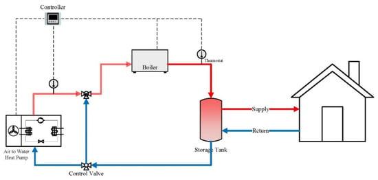
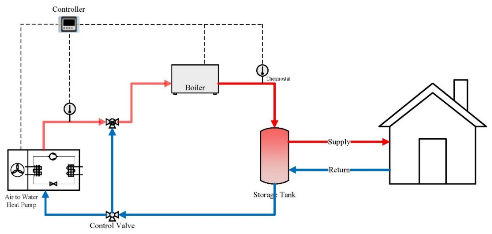
The layout of the simulated system is depicted in Figure 1. The system components were linked by selecting the devices from TRNSYS libraries (called types). The authors customized some types to simulate real processes, such as defrosting (type 581). The simulated AWHP is an inverter-driven system whose behavior is modeled using a performance-map methodology reported in [42]. The manufacturers provide those maps and estimate two AWHP outputs (capacity, in kW; and COP) as a function of three inputs: inverter frequency (ϕ), supply water temperature (Two), and ambient temperature (Text). To ensure flexible, reliable operation and full coverage of heating demand, a BB is coupled with the AWHP. The BB performance is represented in TRNSYS using Type 751, which incorporates average efficiency curves derived from several commercial biomass boilers. These curves depend on water outlet temperature, excess air level, and part-load ratio, and are consistent with the requirements of UNE-EN 303-5:2022+A1 and the European standard EN 303 [43]. The control scheme adopted in this study follows the approach proposed in [40], in which both the AWHP and BB are managed by PID controllers (Type 23) integrated with on–off control logic (Type 2).
Figure 1.
Layout of the hybrid heat pump integrated with a biomass boiler.
2.2. Building Modeling and Climatic Data
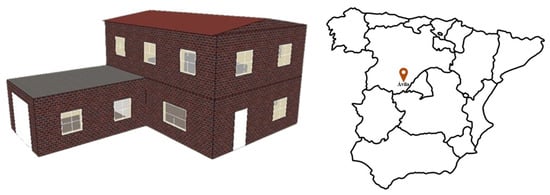
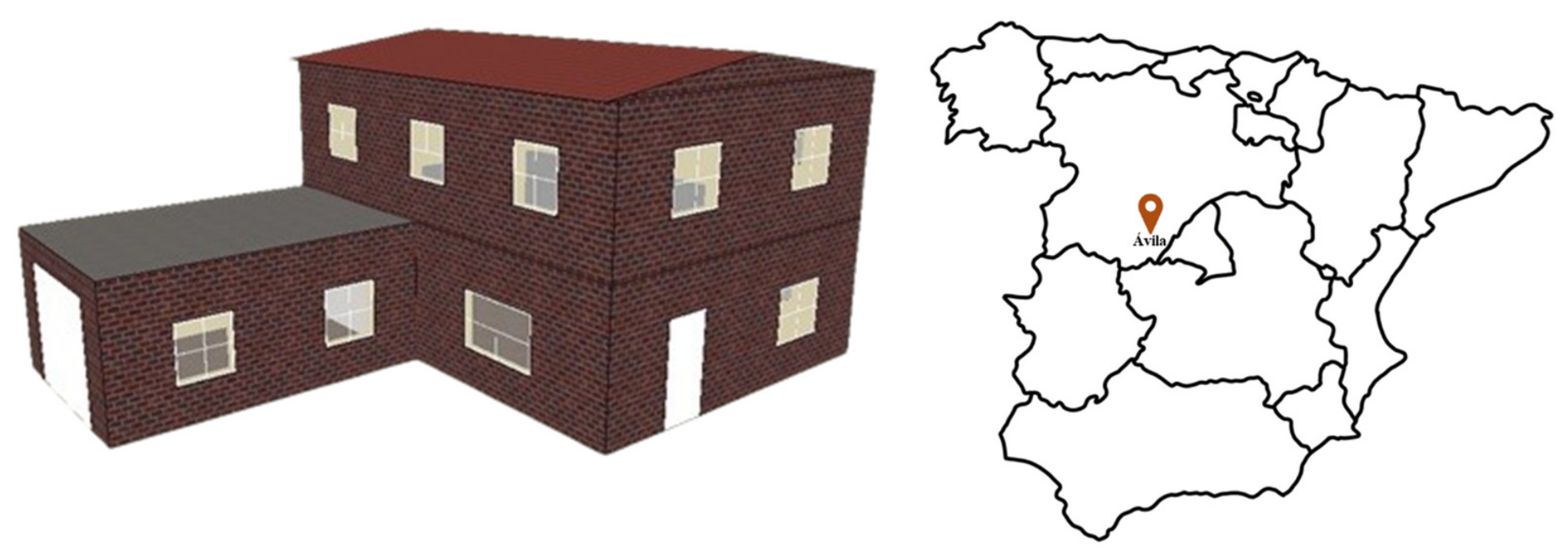
Heating and cooling load demands were estimated by DesignBuilder (v3.2). The details of the building energy model, including geometric characteristics, envelope U-values, infiltration rates, and other simulation inputs, have been thoroughly documented in Refs. [40,44]. The building’s annual heating and cooling demands are 25,458 kWh and 635 kWh, respectively, with peak demands of 12.76 kW for heating and 4 kW for cooling. Indoor temperatures were set at 20 °C from 8:00 to 22:00 and lowered to 17 °C at night, resulting in a heating peak at 8:00 due to colder outdoor temperatures and a 3 °C increase in the target. The demand calculations were based on the climate of Ávila, Spain, classified as Cfb (oceanic climate) with continental influences, characterized by mild summers and acclimatized winters. Hourly demands were integrated into TRNSYS, incorporating local temperature and humidity data to account for part-load operation and the activation of the reverse cycle to defrost the AWHP evaporator. The schematic of the modeled building is shown in Figure 2.
Figure 2.
Schematic of the modeled building and its location.
2.3. Heating System Configurations
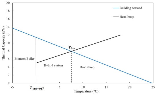
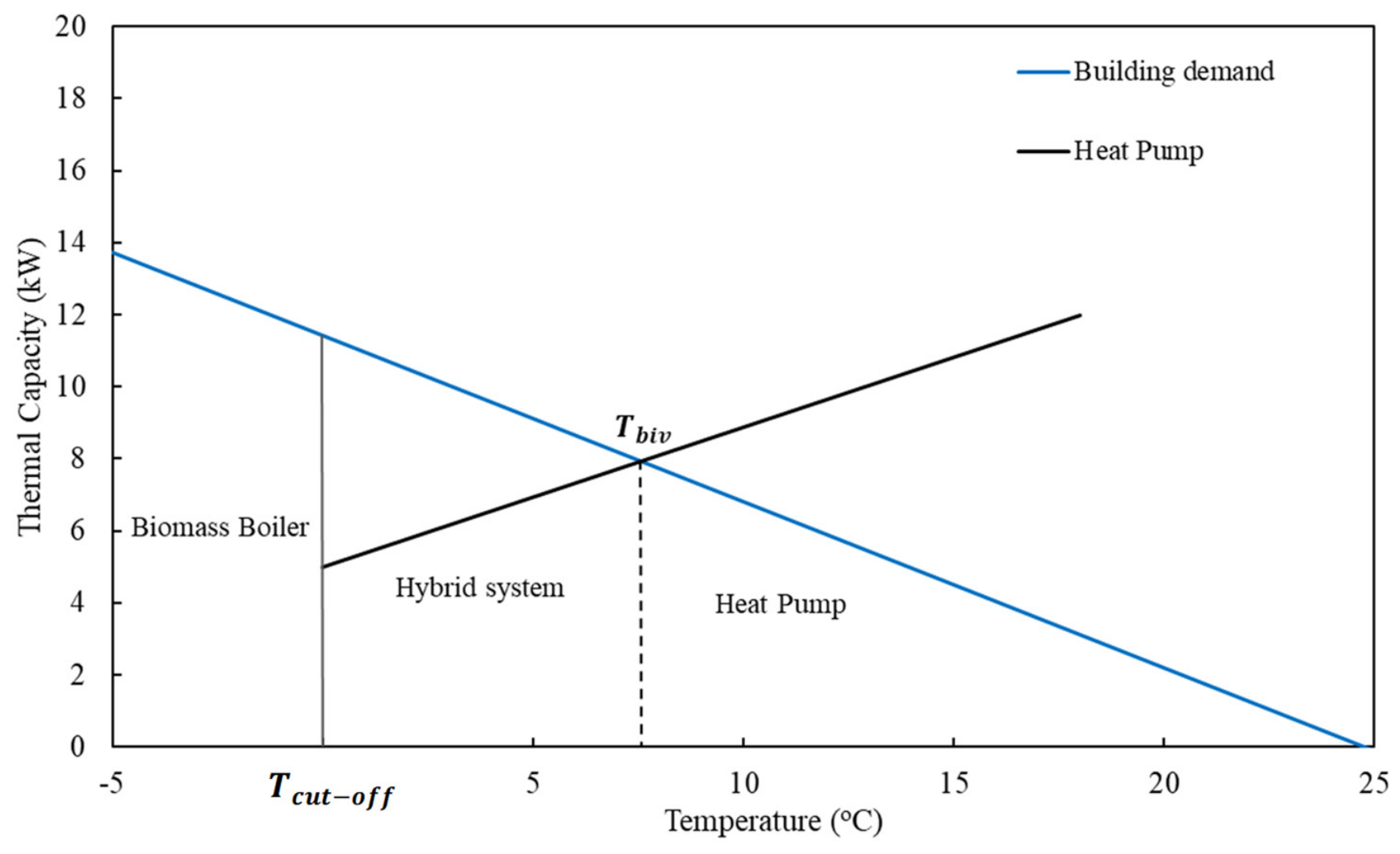
The hybrid system designed to meet the building’s heating demand consists of a BB with capacity fully matching the building’s requirements, while the AWHP capacity is initially set at 6 kW. Figure 3 illustrates the system’s operational mode, showing how the building’s heating demand is partly covered by AWHP, BB, or both, depending on the ambient temperature. The bivalent temperature Tbiv is that one at which the building’s heating demand is equal to the AWHP’s capacity at that outdoor condition. In contrast, Tcut-off is the one at which the manufacturer switches off the AWHP for security or low performance. Then, the HHP system operates as follows:
Figure 3.
The operating mode of the HHP for a given AWHP depends on the ambient temperature.
For : Both the AWHP and BB are active.
For : The AWHP shuts down, and the BB is the sole heating source.
For : The AWHP operates alone, with the BB remaining off.
This approach ensures an efficient balance between AWHP and BB operation based on outdoor conditions.
2.4. Key Performance Indicators
The performance assessment presented in this study relies on a series of key performance indicators (KPIs) previously proposed by the authors and derived from the methodologies outlined in EN 14825 [45] and IEA guidelines [46]. For completeness, the most relevant KPIs are summarized herein; however, detailed definitions, calculation methods, and discussions are provided in the authors’ earlier works [39,40].
where the Primary Energy Factors (, ) for electricity (e) and biomass (b) for Spain have been taken from [47]. Global Warming Potentials (GWP) for electricity and biomass, including the whole life cycle and the infrastructure required [48], are GWPe = 0.521 and GWPb = 0.041 kWh/kWhFE, respectively. Regarding the externalities, the average value of was the commercial price of biomass pellets in Spain for 2024, and was the hourly electrical price [49] in the free electricity market for that year.
3. Machine Learning
3.1. Data Sets
To develop reliable predictive models, it is essential to gather sufficient, high-quality data. For achieving high-accuracy predictions, the training data must be of superior quality and collected during the processing stage. In this study, the data used to build the heat pump performance prediction model were sourced from commercial catalogs of various companies operating in Spain. The initial database consisted of 1432 operating points extracted from commercial technical documentation. Approximately 10% of the records were excluded due to incomplete information, inconsistent operating conditions, duplicated entries, or reporting errors. The remaining dataset was inspected for outliers and normalized using min-max scaling to improve numerical stability during model training. The input variables considered were outdoor air temperature, water supply temperature, and compressor frequency, while the output variables were the coefficient of performance (COP) and heating capacity. Input ranges are shown in Table 1. The dataset was randomly divided into training (70%), validation (15%), and testing (15%) subsets. The training dataset was used for model fitting, the validation dataset for hyperparameter tuning and model selection, and the testing dataset for the final performance evaluation.
Table 1.
Range of the variables in the database.
3.2. Multiple Linear Regression (MLR) Model
The multiple linear regression (MLR) model predicts the dependent variable from two or more independent variables. The basic structure of this statistical method is expressed in equation [50]:
The model determines the predicted value of the dependent variable y by using the partial regression coefficients , the independent variables (inputs, ), and balances the equation by accounting for the random or unexplained error [51]. Its performance is statistically assessed using metrics such as root mean square error (RMSE), mean absolute error (MAE), the coefficient of variation of root mean squared error (CVRMSE), and the coefficient of determination (R-squared) [52]. The MATLAB R2024b computing environment was employed for this analysis.
3.3. Model Selection
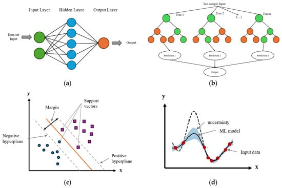
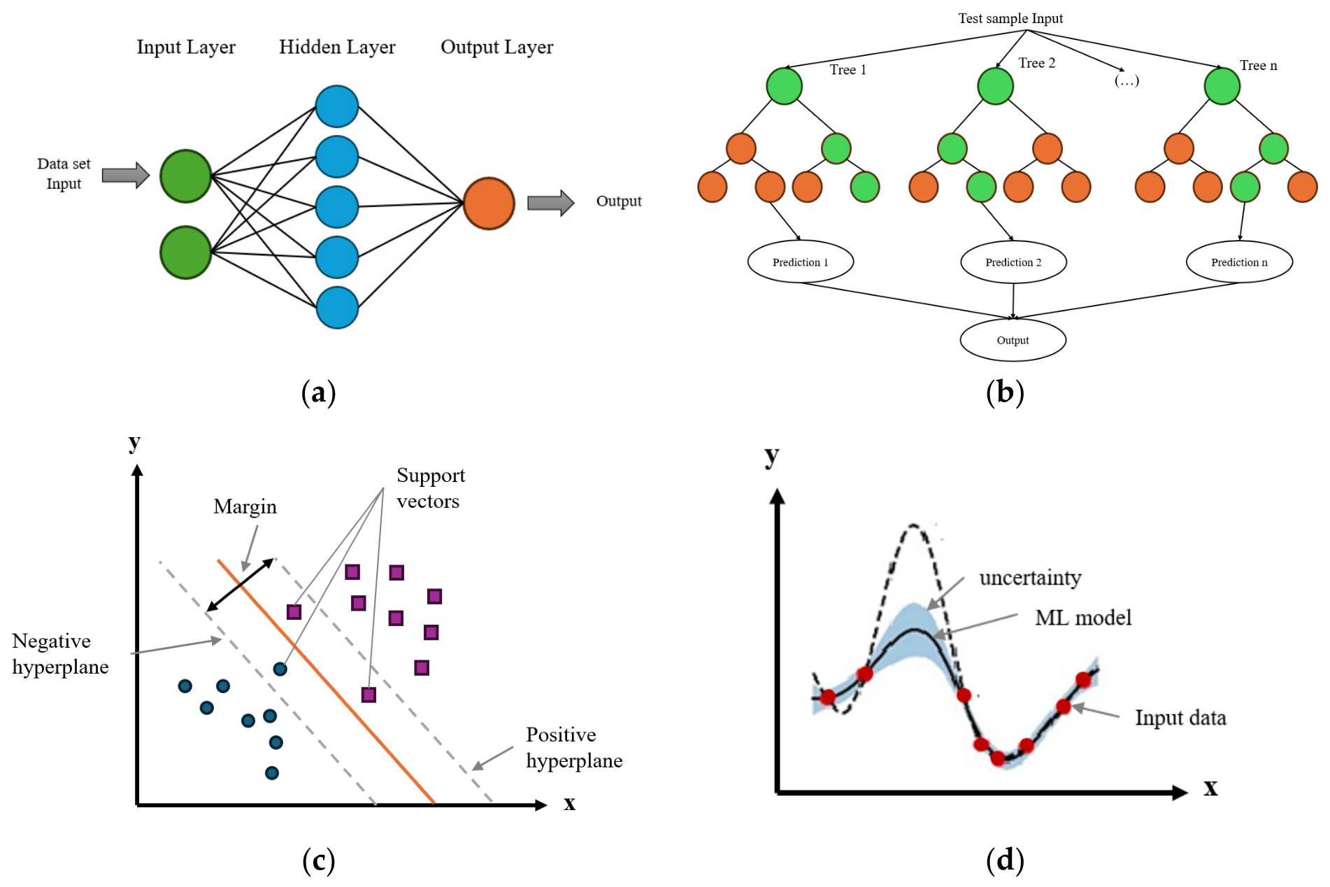
To identify the most appropriate regression model, several widely used data-driven machine learning techniques in building and energy system applications were evaluated, including artificial neural networks (ANN), support vector machines (SVM), Gaussian Processes (GP), and decision trees (DT) (Figure 4). ANNs are multilayer learning models that capture complex nonlinear relationships through weighted connections and backpropagation algorithms [53,54]. SVMs perform regression by determining an optimal hyperplane in a high-dimensional feature space while minimizing prediction errors [55]. GP models provide a probabilistic, non-parametric framework for regression, enabling both predictions and uncertainty quantification through Bayesian inference [56]. DT generates predictions by recursively partitioning the input space; however, they are susceptible to overfitting and instability. To improve predictive performance and robustness, ensemble tree-based methods have been proposed [57].
Figure 4.
Diagram of a machine-learning model. (a) ANN, (b) DT, (c) SVM, (d) GP.
3.4. Evaluation of Prediction Accuracy
Hyperparameters were optimized via an iterative grid search on the validation dataset. The performance of the MLR models is evaluated using error metrics. MAE measures the average magnitude of errors in a set of predictions.
where is the ith measured value, is the ith predicted value, and is the number of observations.
RMSE is the square root of the MSE, which scales the error back to the same units as the target values, making it easier to interpret.
CVRMSE is a metric used to evaluate the average standard error of the predicted RMSE relative to the mean value of the response variable. It is calculated by dividing the RMSE by the average of the observed values.
The coefficient of determination (R2) measures the proportion of variance in the dependent variable explained by the independent variables and indicates the goodness-of-fit between the predicted and observed values.
To reduce the risk of overfitting, model complexity was controlled through regularization techniques and continuous monitoring of training and validation errors. The final model selection was based on predictive accuracy and generalization capability on previously unseen data.
3.5. Prediction Model Development
In this study, a heat pump system performance prediction model was developed using the data collected as outlined in Section 3.1. Specifically, operational data for the heat pump system, gathered from company catalogs, served as the basis for building the predictive model through machine learning techniques. Using data from multiple manufacturers enables the developed model to represent the average performance characteristics of modern air-to-water heat pumps rather than those of a single proprietary product. Consequently, the resulting performance map is intended to provide a generalized representation suitable for dynamic system simulations and comparative analyses.
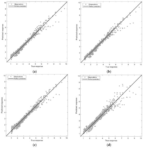
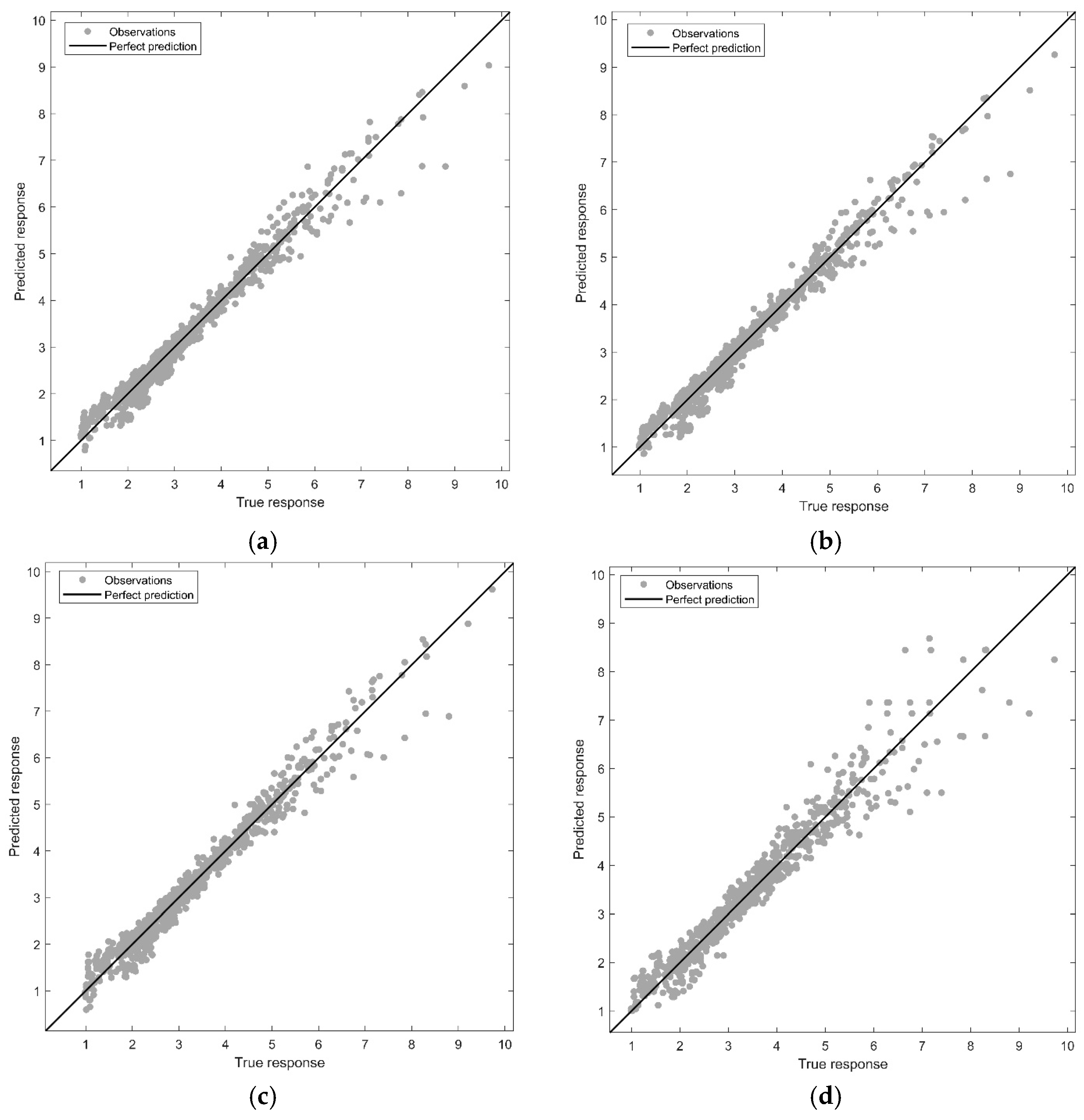
Table 2 presents a comparison between the predicted COP and capacity of the heat pump with the actual values for four different machine learning methods. It highlights the performance of each model, demonstrating their accuracy in predicting heat pump efficiency and capacity based on various feature sets. GP regression performs best, with lower error than other methods. The standard error for all the models is relatively small compared to the range of values. This is illustrated in Figure 5 where the predicted COP values are plotted against the observed values. The plot clearly shows that the predicted COP closely matches the measured values, indicating the accuracy and reliability of the developed models. The ML model exhibited a strong correlation with the training data across different models, as shown in Figure 5. Additionally, it demonstrated strong performance during validation and testing, confirming its reliability in predicting heat pump performance.
Table 2.
Accuracy of the prediction model.
Figure 5.
Plot of COP observed versus predicted. (a) GP, (b) SVM, (c) ANN, and (d) DT.
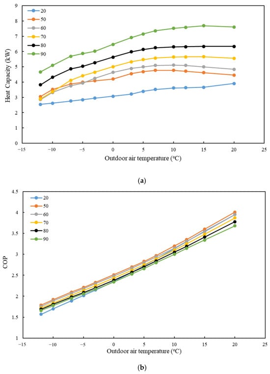
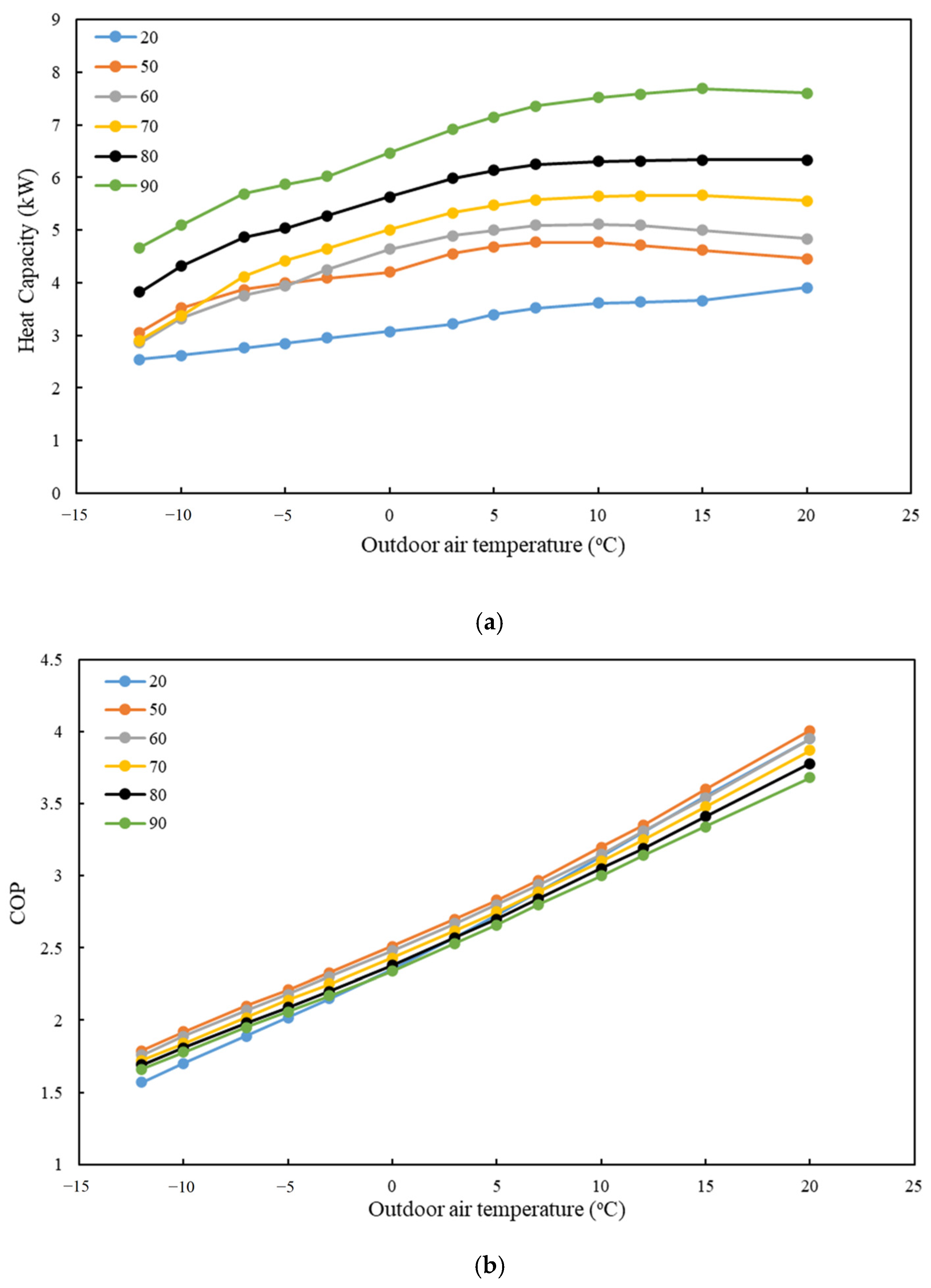
The GP method has been utilized to generate technical data for a new heat pump, which will be used in dynamic simulation. Figure 6 illustrates the predicted heat capacity and COP of the heat pump for full load and partial load, as determined by the machine learning model. These predictions provide valuable insights for heat pump performance in various operating conditions. The trained model was used to generate continuous performance surfaces covering the complete operating range of the AWHP. These surfaces were subsequently converted into lookup tables compatible with the TRNSYS Type 581 heat pump component. During dynamic simulations, TRNSYS calculates the instantaneous operating conditions at each simulation time step and interpolates the corresponding heating capacity and COP from the ML-generated performance map. In this way, the AWHP performance is represented by the trained machine learning model rather than manufacturer-specific performance tables. This approach enables the simulation of a generalized HP representative of current commercial technologies.
Figure 6.
Full and part load AWHP performance data: heating capacity (a) and COP (b). Water supply/return temperature: 55/45 °C.
4. Results
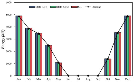
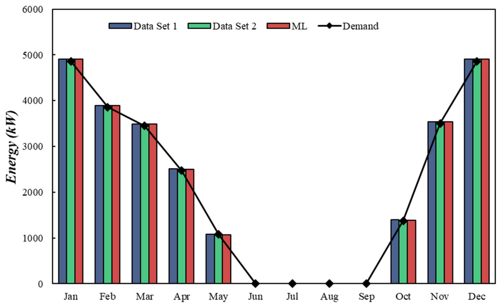
Figure 7 presents the thermal energy supplied by the HHP to the building, along with the demand coverage for the simulated scenarios. The results indicate that all cases, including basic data from companies (data sets 1 and 2) and predicted data from MLR, successfully meet the building’s heating demand throughout the year and perform their functions effectively. Figure 7 shows that the predicted AWHP delivers the same amount of heating to the building as the real data. However, this raises an important question about its performance features compared to real data. Therefore, it is valuable to compare key features, such as ηS on-off cycles, EWI, and operational costs, between the predicted AWHP and the real dataset.
Figure 7.
Thermal energy is delivered to the building.
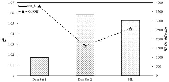
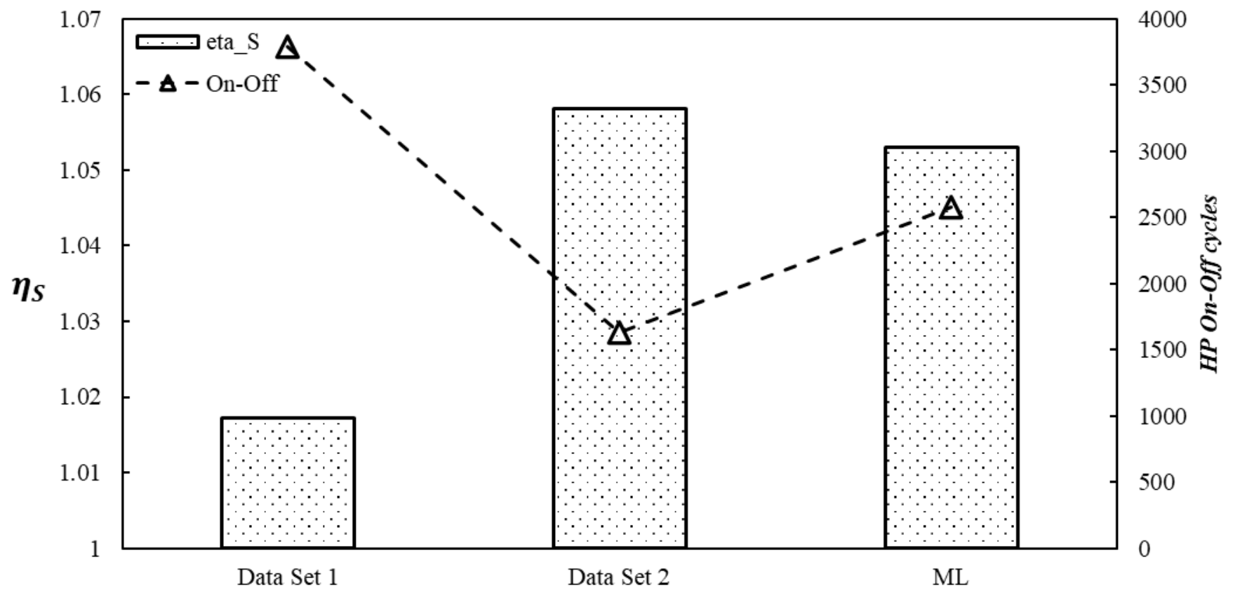
The seasonal energy efficiency of the system (ηS), and the total number of on-off cycles performed by the heat pump are compared for all the simulated cases, with and . The ηS values of the two datasets differ by approximately 5%, while the ML-based AWHP demonstrates performance between them (see Figure 8 for details). The results for on-off cycles show a significant discrepancy of around 55%, and once again, the ML AWHP helps to moderate the difference.
Figure 8.
Comparing real and ML in terms of seasonal energy efficiency of the HHP and the number of on-off cycles of the AWHP.
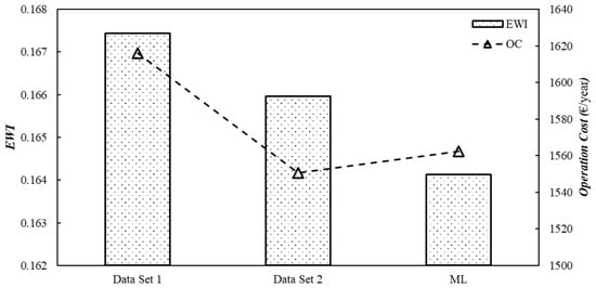
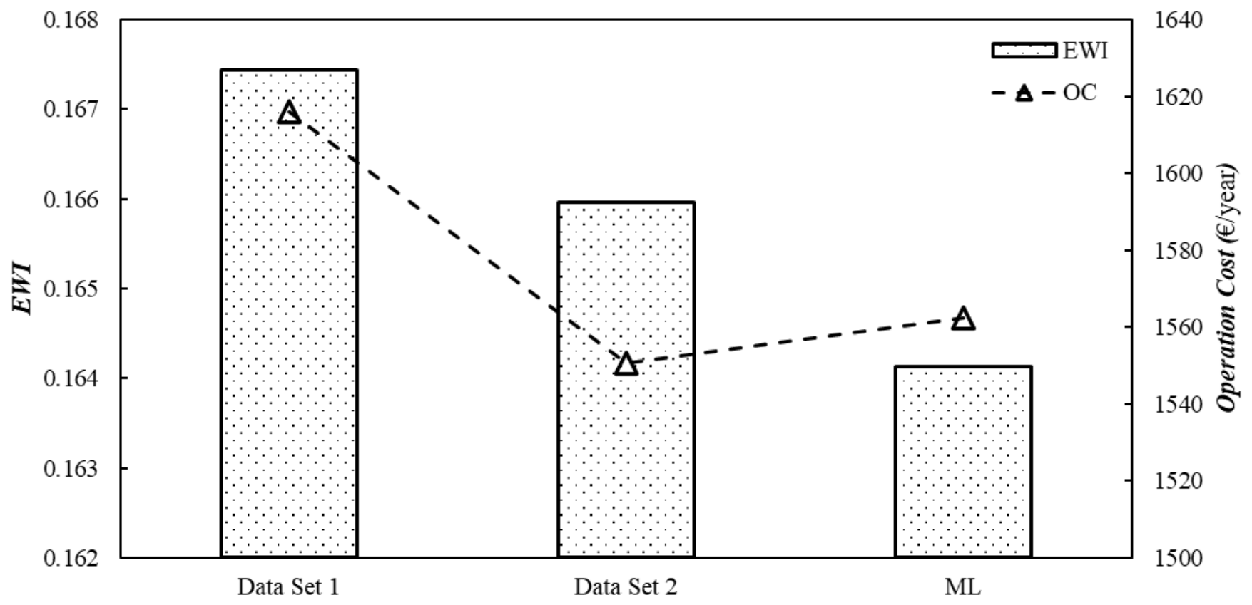
The EWI and the HHS OC for heating and cooling the building are depicted in Figure 9. The EWI considers greenhouse gas emissions from resource consumption, and the lowest value belongs to the ML AWHP. As expected, incorporating the BB reduces the EWI of the HHP system. Indeed, the lowest value observed for the ML AWHP, thus giving the BB greater importance. There is a slight discrepancy in operational costs between the two datasets, with the ML AWHP value falling between the two and closer to dataset 2. This could be explained by the higher ηS observed in dataset 2, which leads to lower OC.
Figure 9.
Comparing the EWI (kgCO2/kWh) and the OC (€/year) with real and ML HHP.
This comparison highlights an important finding: under the same conditions and for the same heat pump capacity, different heat pumps from different manufacturers, while successfully meeting the building’s heating demand, do not exhibit the same performance. Depending on the selected heat pump, different performance interpretations can be derived.
4.1. Effect of Cut-Off Temperature
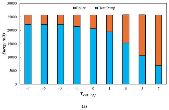
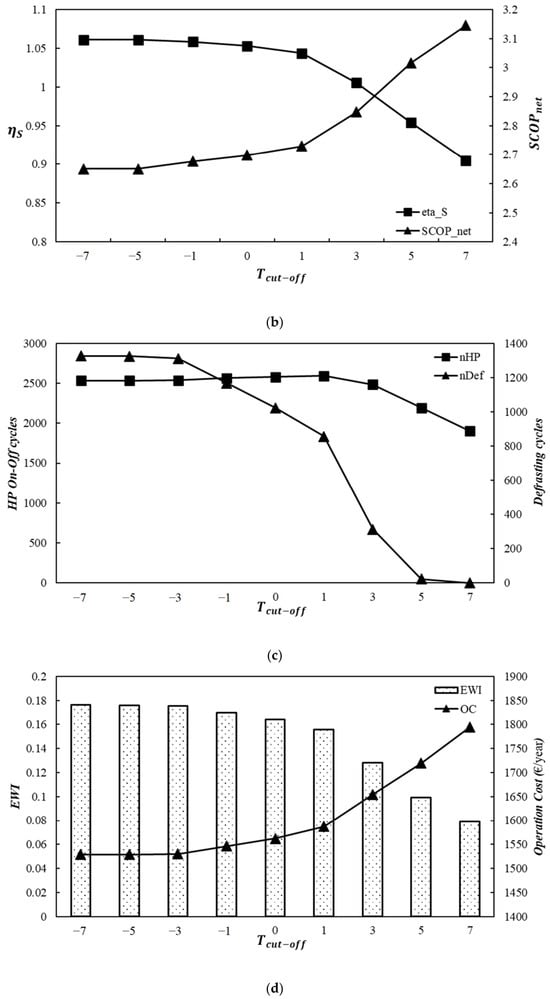
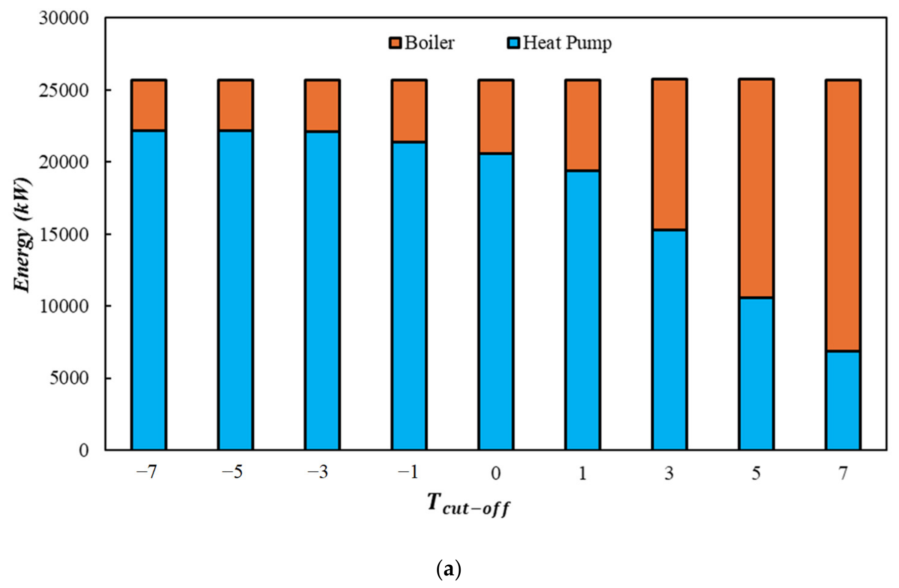
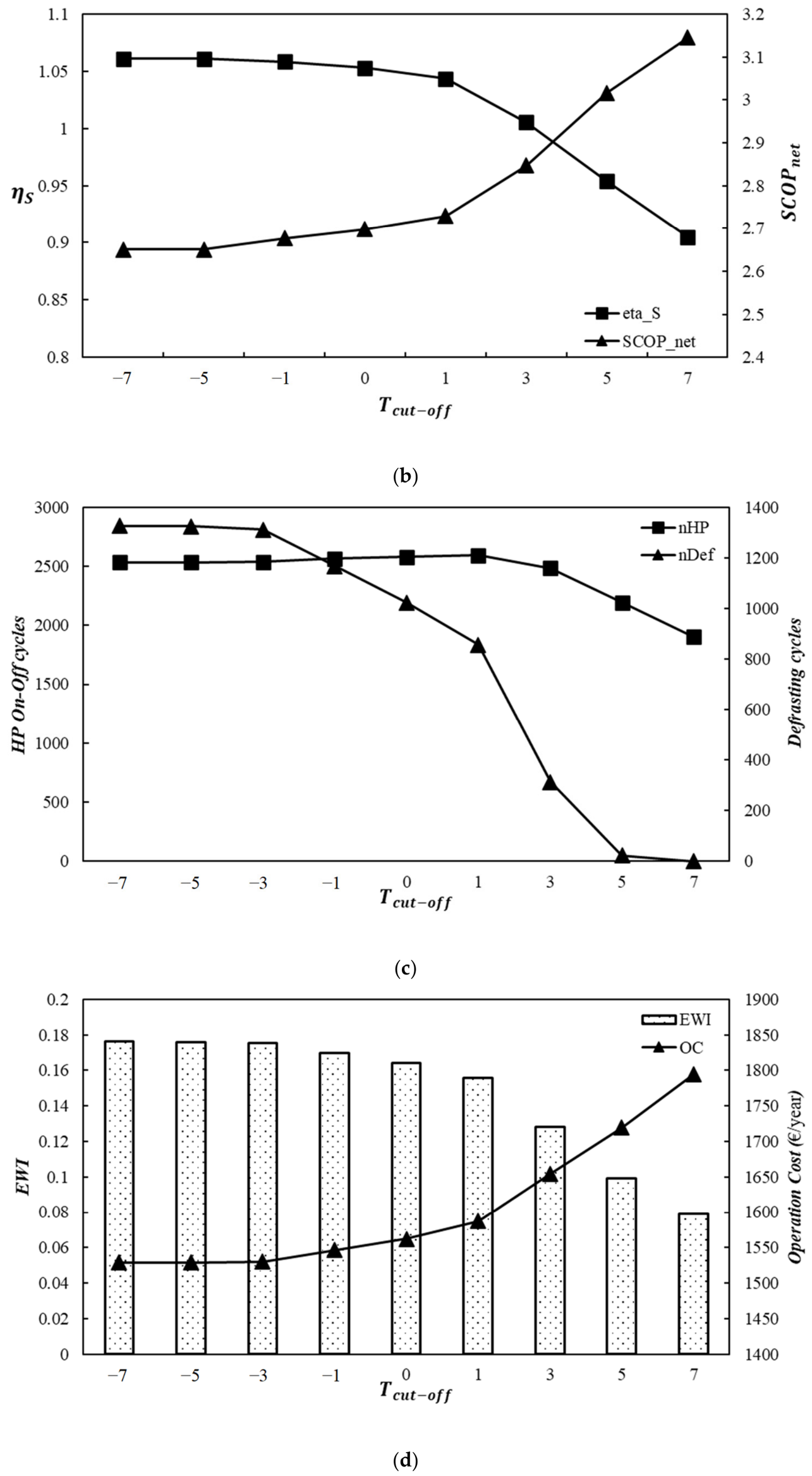
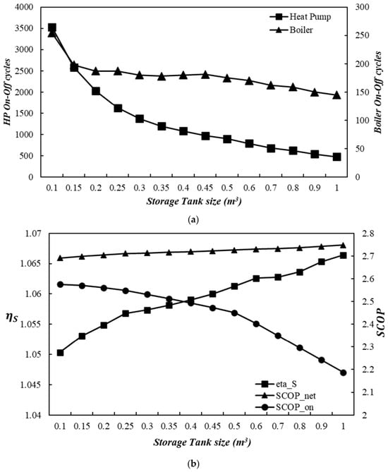
Figure 10 illustrates the effects of the cut-off temperature () and AWHP capacity on the seasonal energy performance and defrosting cycles of the HHP system. Based on the analysis of realistic local weather conditions, was varied from −7 to 7 °C and compared with the baseline case. As increases, the HP’s contribution to the heating demand decreases, while the backup boiler assumes a larger share of the load (Figure 10a). Consequently, the seasonal efficiency () increases with decreasing , whereas the opposite trend is observed for (Figure 10b). This behavior can be attributed to reduced AWHP defrost cycles (Figure 10c) and longer operation of the AWHP at moderate outdoor temperatures, where higher COP values are achieved [58]. Conversely, higher cut-off temperatures increase reliance on the BB to meet heating demand [40]. As a result, the overall system performance becomes more dependent on the boiler efficiency, leading to lower values and higher operating costs (OC). The impact of , on operating cost and environmental impact (EWI) is presented in Figure 10d. Operating costs increase with higher cut-off temperatures because the HHP system’s overall efficiency is lower. In contrast, EWI decreases as the BB contribution increases, reflecting the lower environmental burden associated with biomass-based heat generation.
Figure 10.
The effect of the Tcut-off on some seasonal energy performance indicators: (a) heating participation, (b) and , (c) The number of HP on–off and defrosting cycles, (d) EWI () and operation cost (€/year).
The reduction in defrosting events observed at higher cut-off temperatures is also physically consistent. Frost formation occurs primarily at low outdoor temperatures, which are precisely the conditions avoided when the heat pump is switched off at higher cut-off temperatures. However, the energy savings from fewer defrost cycles are insufficient to offset the increased reliance on the auxiliary boiler. This finding highlights the trade-off between heat pump utilization and auxiliary heating contribution, emphasizing the importance of selecting an optimal cut-off temperature based on both technical and economic criteria.
4.2. Effect of Storage Tank Size
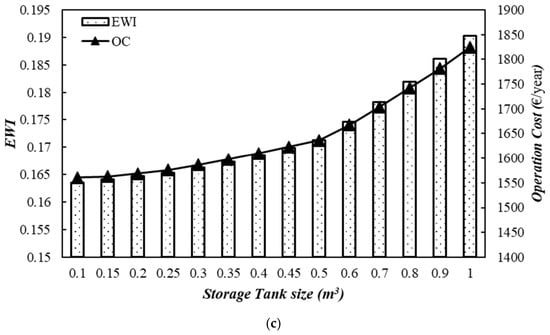
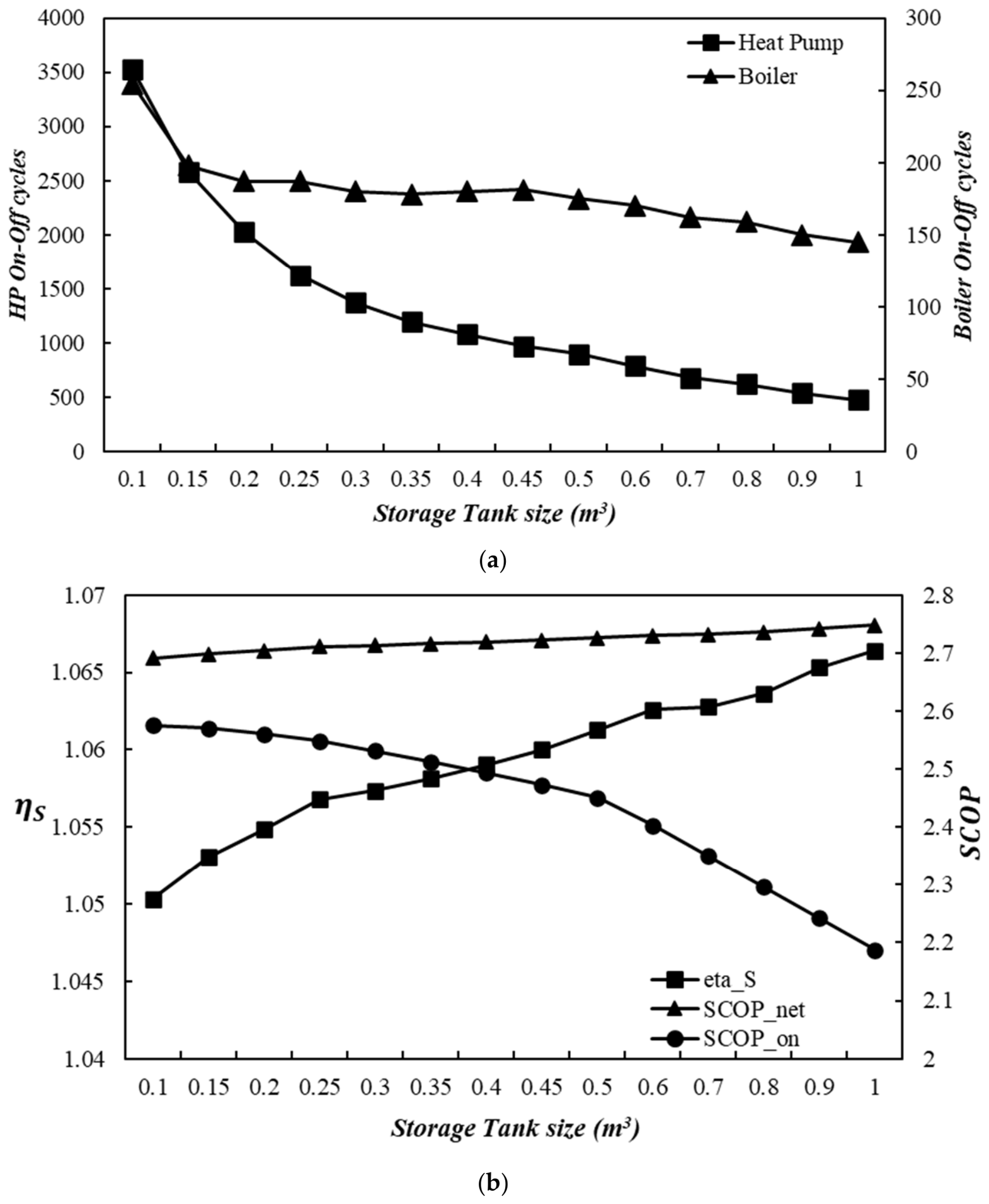
To assess the influence of storage tank size on the seasonal performance of the HHP system, simulations were performed for storage volumes ranging from 0.1 to 1 m3, with a cut-off temperature of 0 °C. As shown in Figure 11a, increasing the storage tank volume reduces the number of on–off cycles of both the AWHP and the BB. This behavior is attributed to the greater thermal storage capacity of larger tanks, which allows energy to be stored for longer periods and delays the temperature drop below the set-point value, thereby reducing cycling frequency.
Figure 11.
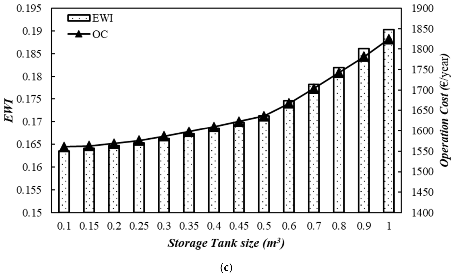
Analysis of tank size on the HHP in terms of (a) on–off cycles, (b) seasonal energy performance, and (c) EWI ().
As shown in Figure 11b, increasing the storage tank volume improves and by reducing heat pump start–stop losses and cycling frequency. Lower cycling rates may also enhance system reliability by reducing mechanical stress. However, decreases with increasing tank size despite the improvement in . This discrepancy is due to the different definitions of the performance indicators: is based on primary energy consumption, whereas reflects final energy efficiency. Larger storage tanks improve primary energy utilization but also increase thermal losses and boiler operation, leading to lower values.
Figure 11c illustrates the impact of storage tank volume on the operational cost and EWI of the HHP system. A slight increase is observed in both metrics as the tank size increases. The decrease in indicates that the system requires more energy input (electricity + biomass) to produce the same amount of heat. As a result, operational costs, which depend on energy consumption, rise, leading to higher CO2 emissions.
4.3. Limitations of the Study
Despite the valuable findings, this study is subject to several limitations that may affect the applicability of the results. These constraints should be considered when interpreting the outcomes and provide directions for future research. The principal limitations are as follows:
- In this study, the MATLAB regression learner was used for machine learning to predict the AWHP performance map. Other machine learning methods may improve accuracy and provide more precise mapping data for component 581.
- The economic analysis uses local and national energy prices and primary energy factors, both of which are influenced by market fluctuations and geopolitical instability. Additionally, integrating PV supply for the AWHP could significantly reduce HHP operational costs and, consequently, the optimal AWHP size.
- Other required TRNSYS parameters not mentioned here could include the temperature dead bands in the differential controllers that start and stop the AWHP and BB. An in-depth analysis could result in the final size of both units being adjusted to form the HHP.
5. Conclusions
In this study, a hybrid heat pump (HHP) system integrating an AWHP with a BB was simulated to evaluate its heating performance for a rural building. Those simulation results are highly dependent on the performance maps of existing commercial AWHP series and cannot be applied to other manufacturers. To overcome this limitation, ML techniques have been used to generate a generic performance map across several manufacturers, providing an overall behavior of an AWHP based on its selected capacity. MATLAB tools were used to obtain accurate technical data from a commercial AWHP portfolio. This data was then used as a mapping source for component 581 of TRNSYS.
Four ML methods (ANN, SVM, GP, and DT) were evaluated for predicting the AWHP performance map, and the best-performing model was selected. A dynamic model was then employed to evaluate the influence of storage tank size and cut-off temperature on the energy, environmental, and economic performance of the HHP system. The main findings are summarized as follows:
- GP regression outperforms other methods in terms of accuracy, exhibiting the lowest error. As a result, the performance map predicted for the AWHP using GP regression can comprehensively cover all frequency ranges, outlet temperatures, and outdoor conditions.
- Heat pumps from different manufacturers, even with the same capacity, exhibit varying performance. While they all meet the building’s heating demand, their efficiency and operational characteristics differ, leading to different performance interpretations depending on the selected AWHP.
- Increasing the cut-off temperature reduces the heat pump’s contribution to meeting the heating demand, requiring greater reliance on the boiler. Additionally, the number of defrost cycles performed by the AWHP decreases, improving the heat pump’s efficiency (). However, the opposite trend is observed for , which declines as a result.
- Larger storage tank sizes reduce the number of on-off cycles for both the AWHP and BB, thereby improving their efficiency. However, the increased heat loss from the tank negatively affects the parameter, based on final energy consumption and focusing on the efficiency with which the heat pump and boiler deliver heating.
- As future work, further studies will be conducted to explore the impact of storage tank size on load shifting. Integrating a latent storage tank could be an optimal solution for rural buildings. By implementing a charge management strategy for the storage tank, issues related to defrosting cycles and peak load demand can be efficiently managed, leading to reduced operational costs and emissions.
Author Contributions
Conceptualization, methodology, formal analysis, data curation, supervision, project administration, funding acquisition, validation, J.U.; formal analysis, software, investigation, writing—original draft preparation, M.T.J. All authors have read and agreed to the published version of the manuscript.
Funding
This research was funded by the TED2021-131397B-100 R&D project funded by MICIU/AEI/10.13039/501100011033/ and by the “European Union NextGenerationEU/PRTR”.
Institutional Review Board Statement
Not applicable.
Informed Consent Statement
Not applicable.
Data Availability Statement
The raw data supporting the conclusions of this article will be made available by the authors on request.
Acknowledgments
The authors also thank Baxi Climatización S.L.U. and Ferroli España, S.L.U. for allowing us to use their AWHP series in this research.
Conflicts of Interest
The authors declare no conflicts of interest.
Abbreviations
The following abbreviations are used in this manuscript:
| ANNs | Artificial Neural Networks |
| ASHP | Air Source Heat Pump |
| AWHP | Air-to-Water Heat Pump |
| BB | Biomass Boiler |
| C | Cooling demand (kWh) |
| COP | Coefficient Of Performance |
| CHP | Combined Heat and Power |
| CVRMSE | Coefficient of Variation of Root Mean Squared Error |
| DT | Decision Trees |
| E | Electricity (kWh) |
| EHP | Electric (monovalent) Heat Pump |
| EWI | Equivalent Warming Impact (kgCO2/kWh) |
| GWP | Global Warming Potential |
| GP | Gaussian Process |
| H | Heating demand (kWh) |
| HHP | Hybrid Heat Pump |
| HP | Heat Pump |
| KPI | Key Performance Indicator |
| IEA | International Energy Agency |
| MAE | Mean Absolute Error |
| ML | Machine Learning |
| OC | Operating Costs (€/y) |
| MLR | Multiple Linear Regression |
| n | Number of observations |
| p | Price (€/unit) |
| PEF | Primary Energy Factor (kWhpe/kWhfe) |
| PID | Proportional-Integral-Derivative |
| PVT | Photovoltaic Thermal collector |
| RMSE | Root Mean Square Error |
| Seasonal Coefficient of Performance (hybrid) | |
| Net Seasonal Coefficient of Performance | |
| SEER | Seasonal Energy Efficiency Ratio |
| SH | Space Heating |
| Seasonal Performance Factor | |
| SVM | Support Vector Machines |
| t | Time (s) |
| T | Temperature (°C) |
| Bivalent temperature (°C) | |
| Cut-off temperature (°C) | |
| Design temperature (°C) | |
| Ambient temperature (°C) | |
| V | Volume (m3) |
| x | Independent variable |
| y | Dependent variable |
| Greek symbols | |
| β | Regression coefficient |
| Heating system seasonal efficiency | |
| Boiler seasonal efficiency | |
| ε | Error |
| Time constant (s) | |
| Part load factor | |
| Inverter frequency (Hz) | |
| Subscripts | |
| b | Biomass, boiler |
| c | Cooling |
| el | Electricity |
| ext | External |
| fe | Final energy |
| h | Heating |
| j | Index |
| o | Outlet |
| pe | Primary energy |
| s | Seasonal |
| set | Set-point |
| th | Thermal |
| tot | Total |
| w | Water |
References
- Huo, T.; Ma, Y.; Cai, W.; Liu, B.; Mu, L. Will the Urbanization Process Influence the Peak of Carbon Emissions in the Building Sector? A Dynamic Scenario Simulation. Energy Build. 2021, 232, 110590. [Google Scholar] [CrossRef] [Scilit]
- Cabeza, L.F.; Chafer, M. Technological Options and Strategies Towards Zero Energy Buildings Contributing to Climate Change Mitigation: A Systematic Review. Energy Build. 2020, 219, 110009. [Google Scholar] [CrossRef] [Scilit]
- International Energy Agency. The Future of Cooling. Available online: https://www.iea.org/reports/the-future-of-cooling (accessed on 15 May 2022).
- Owrak, M.; Aminy, M.; Tajik Jamal-Abad, M.; Dehghan, M. Experiments and Simulations on the Thermal Performance of a Sunspace Attached to a Room Including Heat-Storing Porous Bed and Water Tanks. Build. Environ. 2015, 92, 142–151. [Google Scholar] [CrossRef] [Scilit]
- Tajik Jamal-Abad, M.; Saedodin, S.; Aminy, M. Heat Transfer in Concentrated Solar Air-Heaters Filled with a Porous Medium with Radiation Effects: A Perturbation Solution. Renew. Energy 2016, 91, 147–154. [Google Scholar] [CrossRef] [Scilit]
- Jamal-Abad, M.T.; Saedodin, S.; Aminy, M. Experimental Investigation on a Solar Parabolic Trough Collector for Absorber Tube Filled with Porous Media. Renew. Energy 2017, 107, 156–163. [Google Scholar] [CrossRef] [Scilit]
- Xu, W.; Liu, C.; Li, A.; Li, J.; Qiao, B. Feasibility and Performance Study on Hybrid Air Source Heat Pump System for Ultra-Low Energy Building in Severe Cold Region of China. Renew. Energy 2020, 146, 2124–2133. [Google Scholar] [CrossRef] [Scilit]
- Xu, Y.; Guo, Z.; Yuan, C. Feasibility Study of an Integrated Air Source Heat Pump Water Heater/Chillers and Exhaust Gas Boiler Heating System for Swimming Pool on Luxury Cruise Ship. Energy Rep. 2022, 8, 1260–1282. [Google Scholar] [CrossRef] [Scilit]
- Liu, C.; Han, W.; Wang, Z.; Zhang, N.; Kang, Q.; Liu, M. Proposal and Assessment of a New Solar Space Heating System by Integrating an Absorption-Compression Heat Pump. Appl. Energy 2021, 294, 116966. [Google Scholar] [CrossRef] [Scilit]
- Kozarcanin, S.; Hanna, R.; Staffell, I.; Gross, R.; Andresen, G.B. Impact of Climate Change on the Cost-Optimal Mix of Decentralised Heat Pump and Gas Boiler Technologies in Europe. Energy Policy 2020, 140, 111386. [Google Scholar] [CrossRef] [Scilit]
- Wang, X.; Cui, P.; Zhang, W.; Zhou, X.; Li, L. Optimal Design Methods and Experimental Validation for Hybrid Ground Source Heat Pump System with Gas Boiler. Procedia Eng. 2017, 205, 4149–4156. [Google Scholar] [CrossRef] [Scilit]
- Dongellini, M.; Naldi, C.; Morini, G.L. Sizing Effects on the Energy Performance of Reversible Air-Source Heat Pumps for Office Buildings. Appl. Therm. Eng. 2017, 114, 1073–1081. [Google Scholar] [CrossRef] [Scilit]
- Jarre, M.; Noussan, M.; Poggio, A.; Simonetti, M. Opportunities for Heat Pumps Adoption in Existing Buildings: Real-Data Analysis and Numerical Simulation. Energy Procedia 2017, 134, 499–507. [Google Scholar] [CrossRef] [Scilit]
- Chargui, R.; Sammouda, H. Modeling of a Residential House Coupled with a Dual Source Heat Pump Using TRNSYS Software. Energy Convers. Manag. 2014, 81, 384–399. [Google Scholar] [CrossRef] [Scilit]
- Bagarella, G.; Lazzarin, R.; Noro, M. Annual Simulation, Energy and Economic Analysis of Hybrid Heat Pump Systems for Residential Buildings. Appl. Therm. Eng. 2016, 99, 485–494. [Google Scholar] [CrossRef] [Scilit]
- Bagarella, G.; Lazzarin, R.; Noro, M. Sizing Strategy of On-Off and Modulating Heat Pump Systems Based on Annual Energy Analysis. Int. J. Refrig. 2016, 65, 183–193. [Google Scholar] [CrossRef] [Scilit]
- Deng, S.; Zhang, H.; Li, G.; Qu, T.; Shao, H.; Zhao, Q. Experimental Study and Optimization Analysis of Vapor Compression Heat Pump Coupled with Gas Boiler. Energy 2025, 314, 134189. [Google Scholar] [CrossRef] [Scilit]
- Wu, P.; Wang, Z.; Li, X.; Xu, Z.; Yang, Y.; Yang, Q. Energy-Saving Analysis of Air Source Heat Pump Integrated with a Water Storage Tank for Heating Applications. Build. Environ. 2020, 180, 107029. [Google Scholar] [CrossRef] [Scilit]
- Yu, M.; Li, S.; Zhang, X.; Zhao, Y. Techno-Economic Analysis of Air Source Heat Pump Combined with Latent Thermal Energy Storage Applied for Space Heating in China. Appl. Therm. Eng. 2021, 185, 116434. [Google Scholar] [CrossRef] [Scilit]
- D’Ettorre, F.; De Rosa, M.; Conti, P.; Testi, D.; Finn, D. Mapping the Energy Flexibility Potential of Single Buildings Equipped with Optimally Controlled Heat Pump, Gas Boilers, and Thermal Storage. Sustain. Cities Soc. 2019, 50, 101689. [Google Scholar] [CrossRef] [Scilit]
- Kelly, N.J.; Tuohy, P.G.; Hawkes, A.D. Performance Assessment of Tariff-Based Air Source Heat Pump Load Shifting in a UK Detached Dwelling Featuring Phase Change-Enhanced Buffering. Appl. Therm. Eng. 2014, 71, 809–820. [Google Scholar] [CrossRef] [Scilit]
- Bae, S.; Chae, S.; Nam, Y. Performance Analysis of Integrated Photovoltaic-Thermal and Air Source Heat Pump System through Energy Simulation. Energies 2022, 15, 528. [Google Scholar] [CrossRef] [Scilit]
- Zheng, C.; You, S.; Zhang, H.; Liu, Z.; Zheng, W.; Wu, Z.; Fan, M. Defrosting Performance Improvement of Air-Source Heat Pump Combined Refrigerant Direct-Condensation Radiant Floor Heating System with Phase Change Material. Energies 2020, 13, 4594. [Google Scholar] [CrossRef] [Scilit]
- Li, Y.; Zhang, N.; Ding, Z. Investigation on the Energy Performance of Using Air-Source Heat Pump to Charge PCM Storage Tank. J. Energy Storage 2020, 28, 101270. [Google Scholar] [CrossRef] [Scilit]
- Zheng, X.; Tang, Z.; Wang, Y.; Liu, H. Performance of the air source heat pump assisted solar heating system combined with PCM floor. Appl. Therm. Eng. 2024, 239, 122115. [Google Scholar] [CrossRef] [Scilit]
- Tajik Jamalabad, M.; Abohamzeh, E.; Minhas, D.M.; Kim, S.; Kim, D.; Yoon, A.; Frey, G. Comparative Assessment of Supervised Machine Learning Models for Predicting Water Uptake in Sorption-Based Thermal Energy Storage. Energies 2026, 19, 1619. [Google Scholar] [CrossRef] [Scilit]
- Mitra, S.; Lim, S.; Karathanasopoulos, A. Regression-Based Scenario Generation: Applications for Performance Management. Oper. Res. Perspect. 2019, 6, 100095. [Google Scholar] [CrossRef] [Scilit]
- Bagirov, A.; Mahmood, A.; Barton, A. Prediction of Monthly Rainfall in Victoria, Australia: Clusterwise Linear Regression Approach. Atmos. Res. 2017, 188, 20–29. [Google Scholar] [CrossRef] [Scilit]
- Tomlinson, S. The Mathematics of Thermal Sub-Optimality: Nonlinear Regression Characterization of Thermal Performance of Reptile Metabolic Rates. J. Therm. Biol. 2019, 81, 49–58. [Google Scholar] [CrossRef] [Scilit] [PubMed]
- Badnjevic, A.; Pokvic, L.; Hasici, M.; Bandić, L.; Mašetić, Z.; Kovačević, Ž.; Kevrić, J.; Pecchia, L. Evidence-Based Clinical Engineering: Machine Learning Algorithms for Prediction of Defibrillator Performance. Biomed. Signal Process. Control 2019, 54, 101629. [Google Scholar] [CrossRef] [Scilit]
- Xu, X.; Liu, J.; Wang, Y.; Xu, J.; Bao, J. Performance Evaluation of Ground Source Heat Pump Using Linear and Nonlinear Regressions and Artificial Neural Networks. Appl. Therm. Eng. 2020, 180, 115914. [Google Scholar] [CrossRef] [Scilit]
- Mohanraj, M.; Jayaraj, S.; Muraleedharan, C. Applications of Artificial Neural Networks for Refrigeration, Air-Conditioning, and Heat Pump Systems—A Review. Renew. Sustain. Energy Rev. 2012, 16, 1340–1358. [Google Scholar] [CrossRef] [Scilit]
- Neto, A.H.; Fiorelli, F.A.S. Comparison Between Detailed Model Simulation and Artificial Neural Network for Forecasting Building Energy Consumption. Energy Build. 2008, 40, 2169–2176. [Google Scholar] [CrossRef] [Scilit]
- Roy, S.S.; Roy, R.; Balas, V.E. Estimating Heating Load in Buildings Using Multivariate Adaptive Regression Splines, Extreme Learning Machine, a Hybrid Model of MARS and ELM. Renew. Sustain. Energy Rev. 2018, 82, 4256–4268. [Google Scholar] [CrossRef] [Scilit]
- Kneifel, J.; Webb, D. Predicting Energy Performance of a Net-Zero Energy Building: A Statistical Approach. Appl. Energy 2016, 178, 468–483. [Google Scholar] [CrossRef] [Scilit] [PubMed]
- Guo, Y.; Wang, J.; Chen, H.; Li, G.; Liu, J.; Xu, C.; Huang, R.; Huang, Y. Machine Learning-Based Thermal Response Time Ahead Energy Demand Prediction for Building Heating Systems. Appl. Energy 2018, 221, 16–27. [Google Scholar] [CrossRef] [Scilit]
- Chou, J.-S.; Bui, D.-K. Modeling Heating and Cooling Loads by Artificial Intelligence for Energy-Efficient Building Design. Energy Build. 2014, 82, 437–446. [Google Scholar] [CrossRef] [Scilit]
- Fan, C.; Xiao, F.; Zhao, Y. A Short-Term Building Cooling Load Prediction Method Using Deep Learning Algorithms. Appl. Energy 2017, 195, 222–233. [Google Scholar] [CrossRef] [Scilit]
- Uche, J.; Tajik Jamal-Abad, M.; Martínez, A. Evaluating the Efficiency, Economics, and Environmental Impact of Hybrid Heat Pumps Assisted by Biomass Boilers for Spanish Climate Zones. Energy 2025, 325, 136180. [Google Scholar] [CrossRef] [Scilit]
- Uche, J.; Tajik Jamalabad, M.; Martínez, A. Configurational Design of a Hybrid System Based on an Air–Water Heat Pump and Biomass Boiler for a Rural Dwelling. Appl. Sci. 2024, 14, 9840. [Google Scholar] [CrossRef] [Scilit]
- Klein, S.A.; Beckman, W.A.; Mitchell, J.W. TRNSYS 18: A Transient System Simulation Program; Solar Energy Laboratory, University of Wisconsin: Madison, WI, USA, 2019. [Google Scholar]
- Dongellini, M.; Morini, G.L. On-Off Cycling Losses of Reversible Air-to-Water Heat Pump Systems as a Function of the Unit Power Modulation Capacity. Energy Convers. Manag. 2019, 196, 966–978. [Google Scholar] [CrossRef] [Scilit]
- UNE-EN 303-5:2022+A1:2023; Heating Boilers. Part 5: Heating Boilers for Solid Fuels, Manually and Automatically Stoked, Nominal Heat Output of Up to 500 kW. Terminology, Requirements, Testing, and Marking. CTE: Madrid, Spain, 2023. (In Spanish)
- Ministry of Housing. Royal Decree 314/2006, of 17 March, Approving the Technical Building Code. Official State Gazette, 28 March 2006; Volume 74, pp. 11816–11831.
- EN 14825:2016; Air Conditioners, Liquid Chilling Packages and Heat Pumps, with Electrically Driven Compressors, for Space Heating and Cooling—Testing and Rating at Part Load Conditions and Calculation of Seasonal Performance. European Committee for Standardization (CEN): Brussels, Belgium, 2016.
- Malenković, I.; Pärisch, P.; Eicher, S.; Bony, J.; Hartl, M. Definition of Main System Boundaries and Performance Figures for Reporting on SHP Systems: Deliverable B1. International Energy Agency. SHC Task 44/HPP Annex 38. Available online: https://task44.iea-shc.org/publications (accessed on 23 October 2024).
- Ministry of Industry, Energy and Tourism; Ministry of Development. CO2 Emission Factors and Primary Energy Conversion Coefficients for Different Final Energy Sources Consumed in the Building Sector in Spain; Spanish Government: Madrid, Spain, 2014.
- Ecoinvent Association. Ecoinvent Database 3.6, Cut-Off. Available online: http://www.ecoinvent.org (accessed on 23 October 2024).
- Red Eléctrica de España. Hourly Prices for Electricity in Spain: Daily Downloadable Files. Available online: https://www.esios.ree.es/es/descargas (accessed on 25 June 2026).
- Mousazadeh, M.; Khademi, N.; Kabdaşlı, I.; Rezaei, S.; Hajalifard, Z.; Moosakhani, Z. Domestic Greywater Treatment Using Electrocoagulation-Electrooxidation Process: Optimisation and Experimental Approaches. Sci. Rep. 2023, 13, 15852. [Google Scholar] [CrossRef] [Scilit] [PubMed]
- Shakeri, E.; Mousazadeh, M.; Ahmadpari, H.; Kabdasli, I.; Jamali, H.A.; Graca, N.S.; Emamjomeh, M.M. Electrocoagulation-Flotation Treatment Followed by Sedimentation of Carpet Cleaning Wastewater: Optimization of Key Operating Parameters via RSM-CCD. Desalin. Water Treat. 2021, 227, 163–176. [Google Scholar] [CrossRef] [Scilit]
- Wang, S.; Huang, X.; Liu, P.; Zhang, M.; Biljecki, F.; Hu, T.; Fu, X.; Liu, L.; Liu, X.; Wang, R.; et al. Mapping the Landscape and Roadmap of Geospatial Artificial Intelligence (GeoAI) in Quantitative Human Geography: An Extensive Systematic Review. Int. J. Appl. Earth Obs. Geoinf. 2024, 128, 103734. [Google Scholar] [CrossRef] [Scilit]
- Pantic, I.; Paunovic, J.; Cumic, J.; Valjarevic, S.; Petroianu, G.A.; Corridon, P.R. Artificial Neural Networks in Contemporary Toxicology Research. Chem. Biol. Interact. 2023, 369, 110269. [Google Scholar] [CrossRef] [Scilit] [PubMed]
- Gardner, M.W.; Dorling, S.R. Artificial Neural Networks (The Multilayer Perceptron)—A Review of Applications in the Atmospheric Sciences. Atmos. Environ. 1998, 32, 2627–2636. [Google Scholar] [CrossRef] [Scilit]
- Abbod, M.; Mohammad, A. Combined Interaction of Fungicides Binary Mixtures: Experimental Study and Machine Learning-Driven QSAR Modeling. Sci. Rep. 2024, 14, 12700. [Google Scholar] [CrossRef] [Scilit] [PubMed]
- Williams, R.C.E.; Rasmussen, C.K.I. Gaussian Processes for Machine Learning; MIT Press: Cambridge, MA, USA, 2006. [Google Scholar]
- Breiman, L.; Friedman, J.H.; Olshen, R.A.; Stone, C.J. Classification and Regression Trees; Routledge: Boca Raton, FL, USA, 2017. [Google Scholar] [CrossRef] [Scilit]
- Dongellini, M.; Naldi, C.; Morini, G.L. Influence of Sizing Strategy and Control Rules on the Energy Saving Potential of Heat Pump Hybrid Systems in a Residential Building. Energy Convers. Manag. 2021, 235, 114129. [Google Scholar] [CrossRef] [Scilit]

Disclaimer/Publisher’s Note: The statements, opinions and data contained in all publications are solely those of the individual author(s) and contributor(s) and not of MDPI and/or the editor(s). MDPI and/or the editor(s) disclaim responsibility for any injury to people or property resulting from any ideas, methods, instructions or products referred to in the content. |
© 2026 by the authors. Licensee MDPI, Basel, Switzerland. This article is an open access article distributed under the terms and conditions of the Creative Commons Attribution (CC BY) license.