


Featured Application
U-Net outperforms classical classifiers for mapping crop–nitrogen–water co-limitation on Unmanned Aerial Vehicle (UAV) multispectral imagery to guide fertilization and irrigation. Using a U-Net pre-trained with field data from known nitrogen and irrigation treatments, the model precisely delineates spatial patterns of crop nitrogen and water status, providing >70% accuracy for their interaction. This directly supports the grower’s decision to fertilize and irrigate by identifying deficient or imbalanced areas and enabling site-specific management under subtle spatial variation.
Abstract
This study compared unsupervised and supervised machine learning, and deep learning (U-Net) classifiers on Unmanned Aerial Vehicle (UAV) multispectral imagery to identify nitrogen status in potato crops under nitrogen (N) fertilization treatments, irrigation (I), and their interaction (N × I). The U-Net model outperformed all other methods, achieving accuracies for crop nitrogen status of 65–99% in N, 84–100% in I, and 41–82% in N × I treatments, with variation due to different input data. Supervised machine learning also performed well, with Support Vector Machine achieving 53–87, 66–86, and 32–66% respectively, and Random Forest 61–96, 70–81, and 33–65%. Unsupervised K-means yielded the lowest accuracies (47–58, 9–65, and 8–34%), demonstrating necessity of substantial supervision to delineate crop nitrogen and water status. These findings were confirmed by repeated analyses of UAV imagery acquired later in the growing season with consistent results. Comparable classification performance was observed for crop water status and leaf area index at both time points. Despite being demonstrated in a single-field, single-crop framework, the results provide proof of concept for applying deep learning classifiers to detect subtle nitrogen and water stress under field conditions in precision agriculture. Future research could test diverse agroecosystems and growing seasons, alternative deep learning algorithms, and sensor data fusion to improve classification accuracies.
1. Introduction
Nitrogen (N) fertilization and irrigation are usually oversupplied in agricultural fields to buffer erratic weather effects in crop growth, soil variability and application imperfection. However, this oversupply comes at environmental cost of water overuse and nitrate pollution [1]. Therefore, before determining precise rates of application, field variations in crop water and N status need to be accurately quantified [2,3].
Aside the physically based models, numerous machine learning (ML) models (classifiers and regressors) have been tested for quantifying crop N and water status, including Random Forest (RF), decision tree (DT) and Support Vector Machine (SVM) [4,5,6,7]. SVM is non-linear classifier (although not a strict rule) which transforms input data into a higher-dimensional feature space to apply a kernel (the inner product, i.e., similarity, of two data points) with linear regression within this transformed space [8], while DT is a hierarchical model making sequential decisions based on multiple tests conducted on input features, rules and criteria; RF amalgamates multiple randomly selected decision trees whose outcomes are then aggregated to yield the final result [9]. These “conventional” ML models can estimate crop canopy and yield parameters useful for monitoring reasonably well, including leaf area index (LAI) and aboveground biomass, and are able to discriminate different crops in space and time [6,10,11,12,13]. Few studies examined crop N [2,14,15], whereas studies of co-limitation of water and N lag behind the fast increasing capacity to monitor resource use with remote sensing data and ML [16]. Such studies are necessary to improve field management and minimize farm economic and environmental losses.
Most ML algorithms use labeled training data to recognize contexts of the input data, i.e., are supervised [7,17]. Ensuring high-quality and accurate labeled data, e.g., crop or soil properties, is crucial for effective ML models because in agriculture the spatial (e.g., in-field differences) or temporal windows (e.g., period in a season) are subtle and dictated by agroecosystem dynamics [17]. Accurate labeling is also a time-intensive process and procedures have been developed to generate synthetic data for training the models [7,18]. These are semi-supervised deep learning methods which use not only the spectral content of a pixel in an image (pixel-based), but also image properties such as texture, brightness, entropy, and others (object-based), providing additional attributes and enabling extraction of very complex patterns, i.e., segmentation, from large datasets to remarkably improve labeling and classification accuracy [7].
Deep learning frameworks currently excel in image recognition and segmentation tasks [19]. Convolutional neural networks (CNNs) and U-Net have protruded in perfecting computer vision for various purposes [20,21]. The U-Net architecture with its encoder–decoder structure (a type of neural network used to handle sequential data) has been successful in image segmentation tasks for recognition of plants and weed management [22,23], crop organ detection [24,25] and even classification for irrigation systems [26], as well as prediction of soil parameters such as organic carbon and moisture content, and crop parameters [6]. Blekanov et al. [18] designed a U-Net-based framework given input visible (RGB), near-infrared and Normalized Difference Vegetation Index (NDVI) bands to monitor crop N content for different types of agricultural landscapes. Their study showed high monitoring accuracy and pointed out that the widely used red-edge band— pinpointed in many other studies—is not necessarily needed to achieve good quality of segmentation of the N level of crops under field conditions. Crop water and N status and their variation under co-occurring conditions (N fertilization, irrigation) have surprisingly not been studied, despite these two resources imposing the most important abiotic stress in crop production. Low crop N status under agricultural drought conditions, for instance, is due to lack of irrigation and not fertilization [2,3]. Pancorbo et al. [27] proposed simultaneous assessment of crop water and N status under field conditions using crop indices from hyperspectral and thermal sensors, which are complex and expensive, involving extensive pre- and post-processing. To authors’ knowledge, no study systematically compared ML and deep learning algorithms working on multispectral data to reveal potential monitoring tools for crop water and N co-limitation. Moreover, no study has shown the extent of the established superiority of supervised over unsupervised learning for subtle and interacting spatio-temporal variations in crop N and water status under field conditions, where co-limiting stresses and concurrent changes in LAI create classification challenges that have not been previously benchmarked.
The main aim of this study was therefore to compare the accuracy of classifiers differing in their learning ability to detect subtle spatio-temporal N and water contents of potato (Solanum tuberosum) as a test crop. The specific objectives were to: (1) test unsupervised classification as a comparison baseline to detect and quantify water and N content in the potato field; (2) use SVM, RF and U-Net for supervised classification; and (3) compare the effectiveness of each classifier to determine the best approach for quantifying N and water variability in the potato test field. The results of the study shed substantial light on the potential of data-oriented classifiers on multispectral imagery for conventional and novel applications of irrigation and N fertilization. Although the radiometric principles do not vary from year to year, the single-field and single-crop design of the study constrains generalizability of conclusions, yet providing a necessary controlled benchmark to rigorously disentangle the comparative strengths of conventional ML and deep learning architectures under realistic resource co-limiting conditions.
2. Materials and Methods
2.1. Study Site with Experimental Design and Field Data Collection
This study used image data from a field experiment from 2018 conducted in an agricultural field in Denmark (56°31′59.6″ N, 9°24′39.4″ E). Details can be found in [2,28]. In brief, the field experiment was conducted on coarse sandy soil coinciding with the 2018 European drought–heat wave, imposing significant growth constraints [3]. The climate in the study area is maritime and humid, with mild summers, cool winters and moderate seasonal variation. Mean temperatures and precipitation for the growth season (1 May to 30 September) were 16.4 °C and 284 mm in 2018, compared to the respective values of 14.3 °C and 440 mm in 2017, or 14.6 °C and 517 mm in 2019. The test crop potato, variety Oleva is starch cultivar with medium to high N demand and high yield potential, planted and ridged with 15 cm soil in early May and grown until late October. Twenty-four plots of 30 m were arranged in a randomized split-plot design with six treatments, i.e., two N and three irrigation (I) amounts, each replicated four times (Table 1). Irrigation of either full, deficit, or low/null amounts. The N fertilization was either full according to economic optimum recommendation or variable derived by the relation between canopy Ratio Vegetation Index (RVI) and LAI [29] established from data measured in a nearby potato field with plots for yield response to N fertilizer. In mid-season (23 July 2018) and for each plot we measured crop N (kg ha−1; product of N% and dry matter), water status (%) and LAI.
Table 1.
Summary of the field experiment and the mean values (n = 4) of the variables used in this study measured in mid-season. Full description of treatments can be found in [2,28].
2.2. Remote Sensing Platform and Data Acquisition
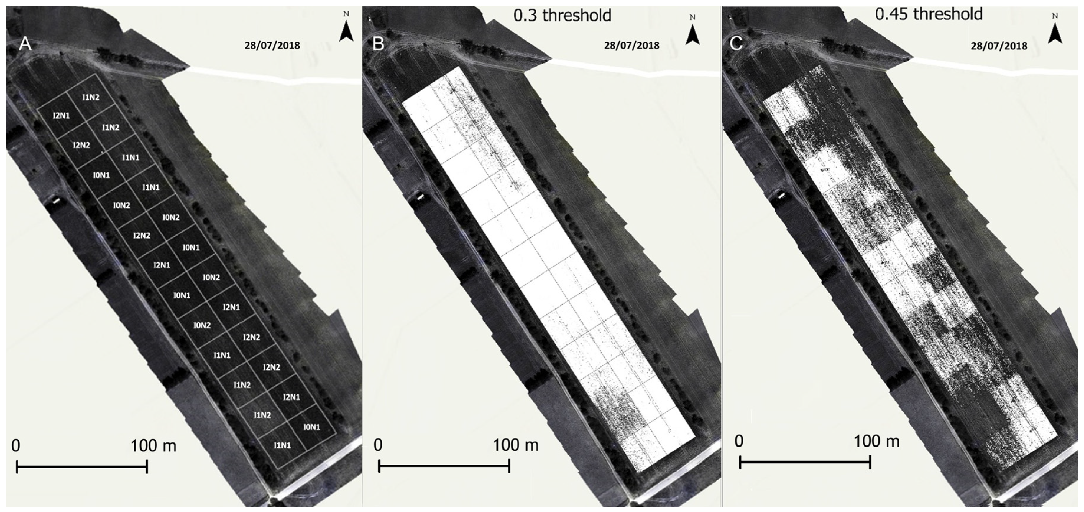
UAV imagery was obtained mid-season on 28 July 2018 and 8 August 2018 to confirm the analysis. At both dates, data were collected by quadcopter UAV Matrice 100 (DJI, SZ, China) flown between 10:00 and 14:00 approximately 60 m above the field at a speed of 6 m s−1 and controlled by Pix4D software on a mobile device. The multispectral camera mounted on the UAV was RedEdge (Micasense, Seattle, WA, USA) with bands consisting of blue, green, red, NIR, and red edge centered at 475, 560, 668, 840, and 717 nm, respectively, with corresponding bandwidths of 20, 20, 10, 40, and 10 nm. Before the UAV campaigns, four to six ground control panels (GCPs) were installed and measured by Trimble RTK GPS. Camera calibration panels were scanned before and after each flight for radiometric calibration. The raw images were processed by Pix4Dmapper (Pix4D S.A., Prilly, Switzerland; version 4.2.27) using the “Ag Multispectral” template for geometric and radiometric calibration. The final mosaic images were resampled to 4 cm spatial resolution (Figure 1).
Figure 1.
Experimental field in Denmark with two nitrogen (1, full, 2, variable) and three irrigation levels (0, full, 1 deficit, 3, nill) replicated four times (A). Soil was masked from canopy pixels using Normalized Difference Red Edge (NDRE) index testing thresholds of 0.30 (B) and 0.45 (C).
2.3. Image Classifications
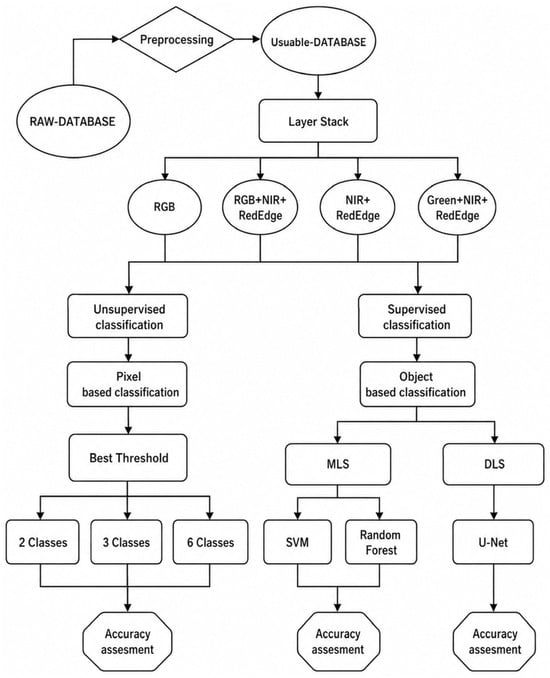
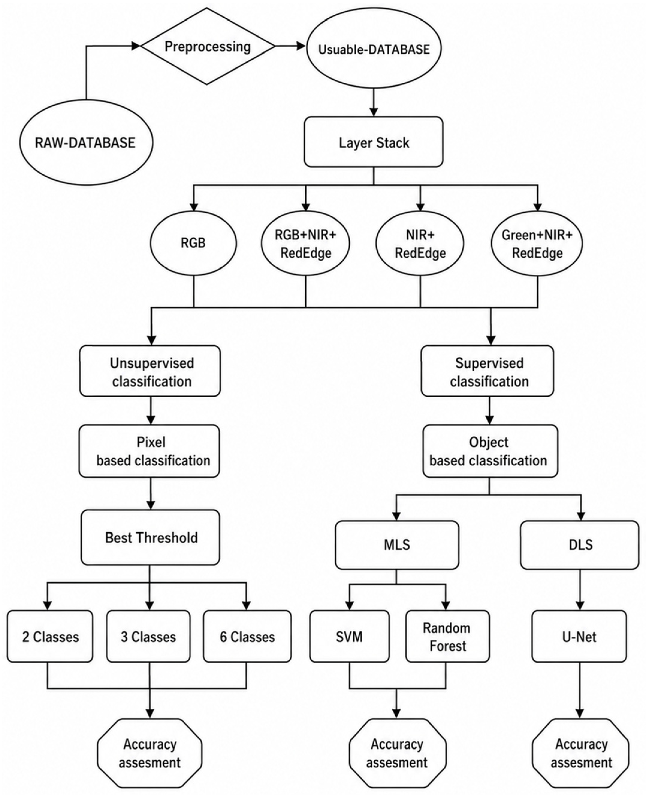
The detailed workflow in the framework for detecting water and N status consisted of remotely sensed data compilation and processing by a series of image classifiers in comparative analysis (Figure 2). First, soil background must be masked from crop canopy. Pixel values exceeding certain thresholds could be deemed bare soil, and a Normalized Difference Red Edge Index (NDRE) is often used because it detects variations in crop health at more advanced stages, using red-edged light that penetrates leaves deeper than red light, making it effective for removing bare and dryer soil [30]. Two NDRE thresholds were tested, 0.3 and 0.45. The 0.3 threshold allowed masking soil without losing unhealthy (i.e., treatment) canopy, which has similar reflectance to soil; however, some soil could not be masked. The 0.45 threshold masked all soil but also resulted in the loss of most unhealthy canopy (Figure 1). Thus, the multispectral images were masked with 0.3 and 0.45 threshold. During the image pre-processing stage, testing additional thresholds always showed that values < 0.30 retain excessive soil pixels, whereas values > 0.45 increasingly excluded canopy pixels, resulting in a marked deterioration of classification quality. Therefore, these two thresholds represented good range to evaluate the influence of soil masking on classification performance. Finally, specific combinations of the masked bands (RGB, RGB + NIR + RedEdge, NIR + RedEdge, NIR + RedEdge + Green) were stacked and used for all classifiers, as described next. To ensure that classification labels reflected true physiological states rather than nominal treatment identifiers, labels were assigned based on the combined ground-truth measurements, i.e., crop nitrogen content, crop water content and LAI (Table 1); treatments with overlapping single-variable values (e.g., similar N content but distinct LAI) were retained as separate classes to capture the multivariate stress imprint recorded by the multispectral sensor. Pixel-level ground truth data were the plots classed as ‘regions of interest’ in all supervised classifications.
Figure 2.
Study workflow. Classes refer to treatment labels in Table 1 as 2 for nitrogen (full or variable), 3 for irrigation (full, medium or low/null) and 6 for the nitrogen and irrigation interaction.
2.3.1. Unsupervised Classification
K-means clustering is an unsupervised classifier that groups unlabeled data into different clusters. This means, the algorithm does not require labeled training data but unlabeled feature vectors (in our case, the treatments) to calculate distances and form clusters. The K in its title represents the number of clusters that will be created and this is the sole human interference with the machine used for algorithm training. The algorithm is centroid-based, meaning that each data point is assigned to the cluster with the closest centroid. In the study, we used ERDAS Imagine 2015 to create a signature set according to the different treatments: 1 = I0N1, 2 = I1N1, 3 = I2N1, 4 = I0N2, 5 = I1N2, and 6 = I2N2.
The unsupervised classification algorithm uses a K-means method with the processing set to a maximum of 10 iterations and a convergence threshold of 0.95, which is standard/default in many remote sensing applications and indicates when the clustering solution has stabilized sufficiently, i.e., 95% of the pixels remain assigned to the same cluster between two successive iterations. The formula for the K-means algorithm is shown below, where represents the objective function:
where k is the number of clusters, n is the number of data points, and j and i represent the clusters and the data point respectively, such that is the i’th data point in cluster j and μj is the centroid of cluster j. The result gets the squared sum of the total distance between the data points and their centroid. Unsupervised classification was performed also for the three I and two N treatments.
2.3.2. Supervised Machine Learning Classification
Supervised ML model predicts outcomes after it has been trained by human on labeled data. Some ML algorithms require more input, others require less. During the training, the model adjusts its weights until it is properly fitted, which is part of a validation process. In our study, SVMs and RF were used, both robust for classification tasks, each with its own strengths. SVM is particularly effective in high-dimensional spaces and is versatile in its kernel trick to handle non-linear classification. RF, on the other hand, is known for its accuracy and ability to handle large datasets with higher dimensionality.
In this study, the initial step involved compilation of the training dataset with Training Sample Manager tool in ArcGIS Pro v.3.0.2. This involves generating three shapefiles for each measured variable (crop N, crop water, LAI). The first shapefile encompassed the six treatments covering an area of 250 m2 (1.1% of plot), summing up to 6.6% for all treatments. The second sampling area represents the three I classes covering approximately 6.6% of the total area, and the third shapefile delineated the two N treatments also covering around 6.6% of the field. The SVM classifier segments the selected image based on specific parameters: spectral detail of 15.5, spatial detail of 15, and minimum segment size of 20 pixels. The model was trained on maximum 500 samples per class. The output was a categorized image featuring crop N, crop water or LAI classified across the treatment plots. This process was repeated for inputs consisting of the RGB UAV imagery, near-infrared and red edge (Nir/RE), added green (Nir/RE/G) and all bands. For RF, to ensure consistency, the segmentation features remain unchanged as the training sample shapefile. Maximum number of trees was set to 50, maximum tree depth to 30, and maximum number of samples per class to 1000. The accuracy of the classifications was evaluated using the same methodology employed in our unsupervised classification analysis.
2.3.3. Supervised Deep Learning Classification
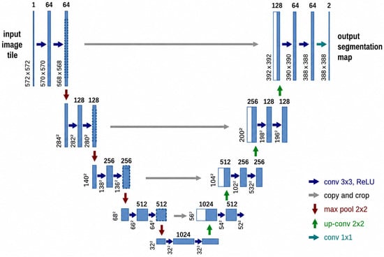
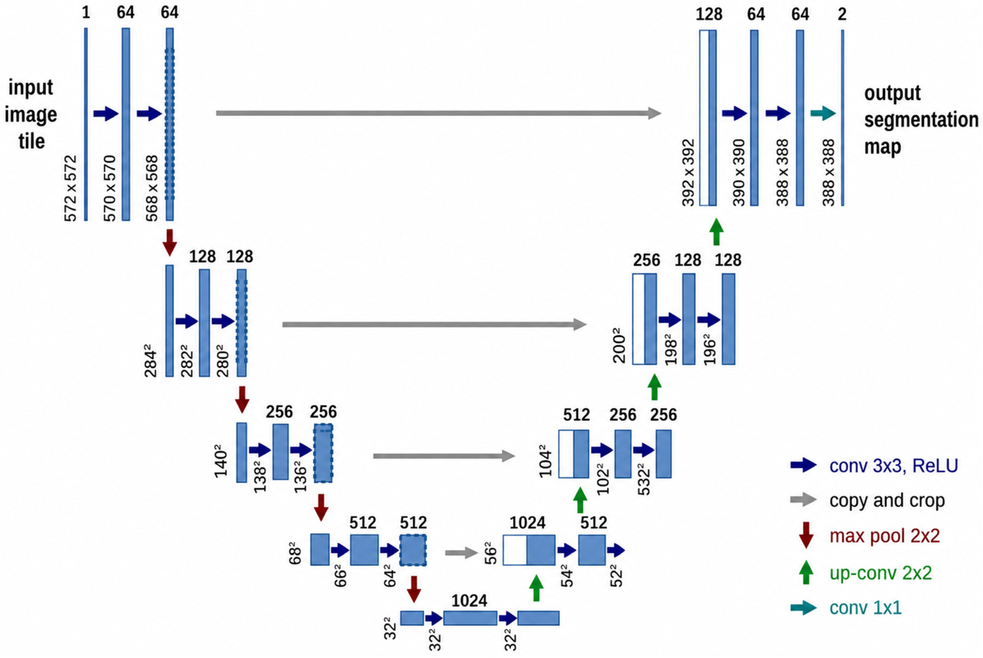
U-Net is convolutional neural network developed for medical image analysis [31], but demonstrated outstanding performance in land cover images [32,33] and has been applied in all disciplines involving image segmentation [4]. U-Net encoder is responsible for feature extraction through a series of convolutions and pooling operations, effectively downsampling the image. The decoder performs upsampling to restore the original image shape and predict each pixel. Skip connections link encoder and decoder, integrating features at different levels in both parts of the network [34]. The neural network is thus named U-Net due to the shape of its architecture resembling the letter U (Figure 3), comprising left/encode and right/decoder side.
Figure 3.
U-Net architecture for image segmentation. Input image tiles are processed through successive 3 × 3 convolutions with ReLU activations and 2 × 2 max pooling in contracting path, followed by 2 × 2 up-convolutions in expanding path with skip connections (copy-crop). Final 1 × 1 convolution creates output segmentation map. Numbers show feature-map size and channels at each level.
2.4. Preprocessing and Deep Learning Algorithm Training
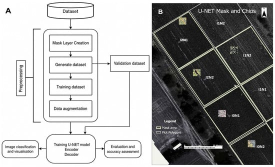
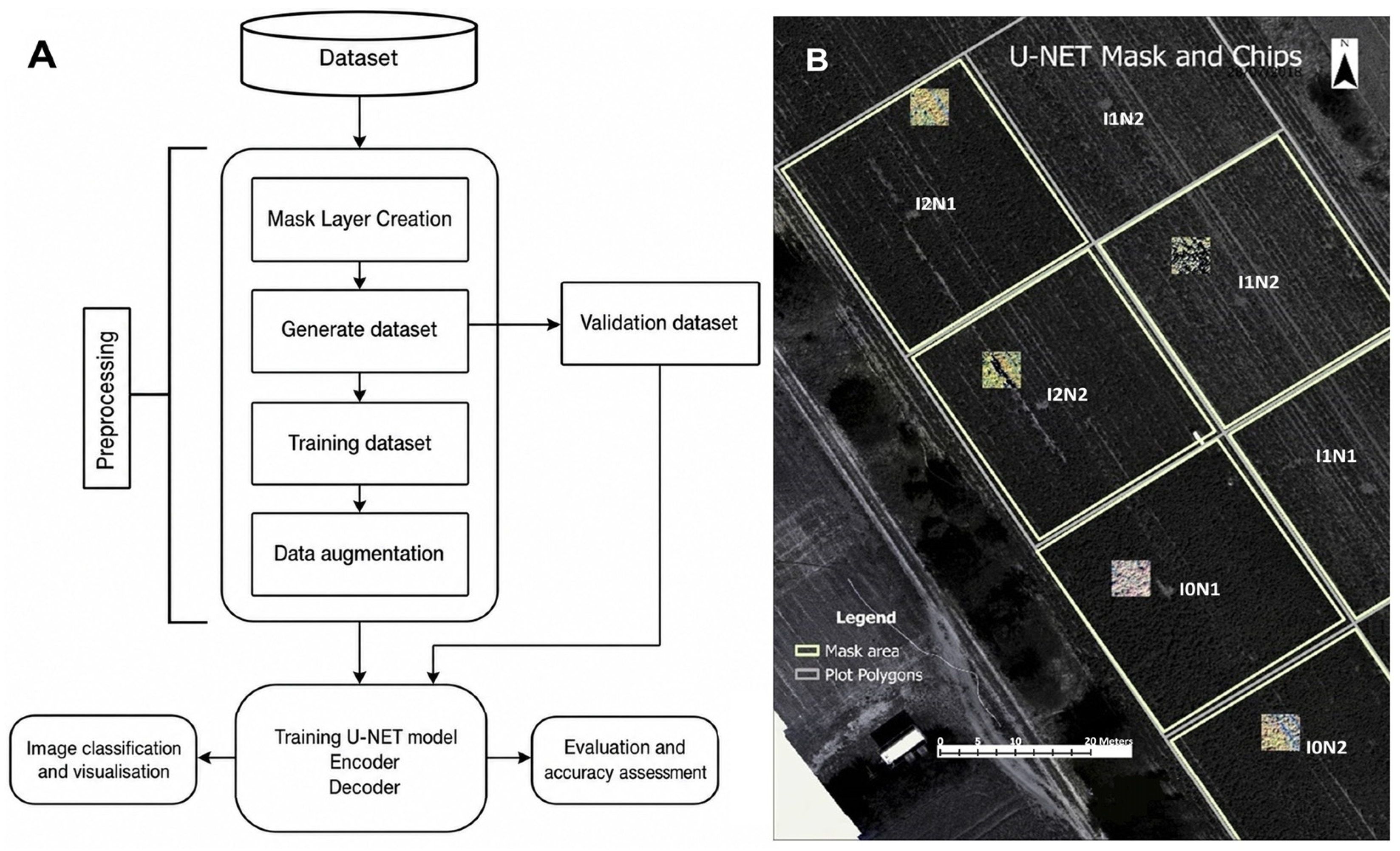
To develop U-Net-ready datasets, a mask layer was created serving as a sampling area for the six treatments. Each class covered 4.1% of the total area on the image, thus 25% of the whole image was used for dataset extraction and training the model (Figure 4). Then the training datasets (i.e., images) were generated, where each training image had a size of 128 × 128 pixels with a stride of 64, resulting in 1748 images in total. Stride is a parameter that dictates the movement of the kernel across the image. When performing a convolution operation, the stride determines how many units the filter shifts at each step, either horizontally, vertically, or both. A larger stride will produce a smaller output dimension, effectively downsampling the image. In this study, a stride of 64 was set. Next, to prepare the dataset, these patches were divided into 80% for machine training and 20% for validation. To enhance robustness of the training process and prevent overfitting, standard augmentation process was applied with the following parameters: rotation range = 90, width shift range = 0.15, height shift range = 0.15, horizontal flip= True, to increase the size of the training dataset to 12,582 during training. The final dataset comprised 12,582 training and 350 validation images. Finally, 20 epochs were set to train and to save the model with the best performance, with a batch size of 8. In deep learning, an epoch represents the number of times a complete training dataset is processed through the network, and batch size refers to number of training examples used in a single iteration of model training. To mitigate the contingency inherent to single training sessions, an early stopping and learning rate decay was conducted based on a fixed validation set (50 images), saving the best-performing checkpoint. Multiple independent training runs from scratch were not performed; this limits the interpretation of the absolute stability of the reported metrics, though to a minor extent.
Figure 4.
U-Net classification pipeline scheme showing the process from dataset compilation to model validation (A) and chips with a size of 164 × 164 extracted from the plots with different treatments and used as input for the U-Net model (B).
2.5. Evaluation and Accuracy Assessment
To evaluate the effectiveness of the models for the treatments’ variable segmentation task, we used the standard metrics: accuracy, precision, recall and F1-score. Accuracy is a metric that indicates how frequently an ML model accurately predicts an outcome. Precision is one metric of an ML model’s performance; it refers to the quality of the model’s positive predictions. Recall, a commonly used performance metric for classification models, is the fraction of positives that are correctly classified. The F1 score is a performance metric for classification and is calculated as the harmonic mean of precision and recall:
where TP, TN, FP and FN, are, respectively, true positives, true negatives, false positives and false negatives.
All algorithms tested in this study use different sampling procedures, training sizes, and tuning processes. Accuracy assessment was done in Python v3.11 in Visual Studio Code v1.96 and two methods were applied for accuracy check. The first method included counting the number of pixels correctly classified within the respective plots of each treatment, and then checking for accuracy in terms of how many plots are successfully classified according to their treatment using a confusion matrix, as shown in the pseudocode:
The second method, a breakdown of the first, calculates the percentage of pixels in each plot and then determine the rate of pixels that represent the treatment/class in which that plot belongs, whether the majority or not. This method demonstrates how many pixels have been accurately classified within the plots as defined by the pseudocode below:
This approach allowed comparison between different classifiers, and also between multiple combinations of bands for each classification method. The threshold with the best accuracy results was selected and used for ML and deep learning classification.
3. Results
3.1. Unsupervised K-Means Clustering
The unsupervised K-means clustering model was first compared using 0.3 and 0.45 thresholds for NDRE to mask soil and predict the six treatment labels, and threshold 0.3 provided better accuracy (see Figure A1, Table A1 in the Appendix A). This threshold was included in the rest of the analysis. The K-means model predicted I and N classes poorly, regardless if individual or interacting treatments and regardless of input bands (Table 2). A similar pattern at a slightly different magnitude of accuracy was seen for the prediction of LAI and crop water status by K-means (see Table A2 and Table A3 in the Appendix A).
Table 2.
Classification accuracy (%, from low/red colour to high/blue colour) of unsupervised (USC; K-means), supervised machine learning (Support Vector Machine, SVM, Random Forest, RF) and deep learning (U-Net) for mid-season nitrogen status of potato. Accuracy’s values for pooled treatments (N, I and N × I) were calculated according to Equation (2), while treatment-specific accuracy values were calculated according to Equation (3). Classes refer to treatment labels in Table 1. RGB, G, RE and Nir are true-color, green, red edge and near-infrared bands of the camera, respectively.
3.2. Machine Learning Classification
The results for SVM and RF for crop N are shown in Table 2; those for LAI and crop water status can be seen in Table A2 and Table A3 in the Appendix A, respectively. For both models and all variables, the lower the number of classes, the higher the accuracy, and more input bands generally increased the accuracy. For all variables, both classifiers performed comparable for I (87 and 81% overall accuracy for SVM and RF respectively) and I × N (65–66% for both classifiers), but for N treatments RF outperformed SVM (96 and 87% accuracy, respectively). For the factorial treatments, both classifiers performed well only for I1N2 and I2N1 (except when RBG was input data). This is interesting as both treatments involved a deficit or no irrigation and very subtle spatial variations with low values for the three variables (Table 1). Also, the band combination with the highest accuracy was G, RE, and NIR, followed by the all-bands combination, while the worst was often the RGB data input.
3.3. Deep Learning U-Net Classification
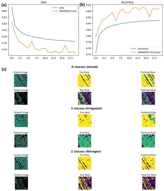
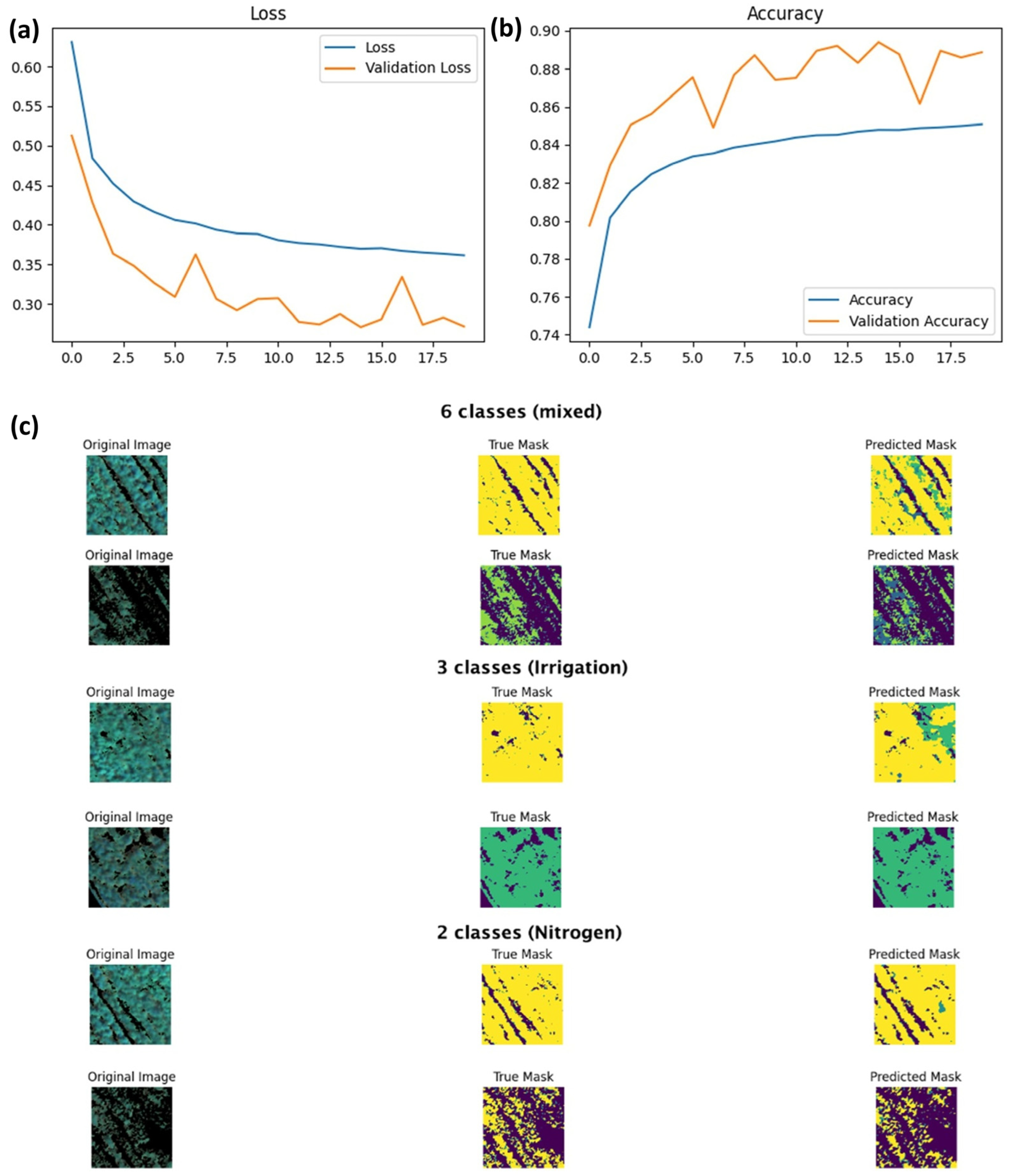
U-Net model exhibited exceptional performance in segmenting the treatments, achieving segmentation accuracy of 70% for the six classes, about 93% for I and 85% for N classes. Training and validation loss and accuracy of the U-Net model are shown in Figure 5a,b with the chart displaying 20 epochs. From this plot, we can understand model performance and learning behavior. The training loss is decreasing gradually, which means the model progressively enhances the performance of the training data (Figure 5c). It decreases with some fluctuations, but overall, it indicates that the model generalizes to the validation set well. The accuracy of the classification itself showed high values (above 60%) for almost all treatments and input bands, except RGB. While the lower end of this accuracy may appear moderate at first glance, the precision, recall, and F1-score summarizing the U-Net model training for 6-treatments segmentation (Table 3) show high precision and recall for most treatments, leading to strong F1-scores. As for I2N1, precision 0.76 and recall 0.85 means an F1-score of 0.80. Therefore, U-Net is robust and fairly accurate for 2–3 treatments classification across different input data for predicting crop N, LAI and water status, compared to the other classifiers. U-Net was able to extract information about canopy N and water content and LAI under drought (treatments with I2), reaching 84% for I2N2 (Table 2). Also, from Table 2 can be seen that U-Net provides 93% overall classification accuracy (correctness of the classification) using RGB imagery, though only for the treatment with optimal production (ample water and split ample nitrogen, I0N2).
Figure 5.
(a) Loss and (b) accuracy of U-Net model and (c) predictions of different treatment classes. On the left is original image, in the middle is image representing the true correct mask (the corresponding class), and on the right is the predicted mask. Classes refer to treatment labels in Table 1.
Table 3.
Precision, recall, and F1 statistics of the U-Net classifier. Classes refer to the treatment labels in Table 1.
3.4. Overall Comparison of Classifiers
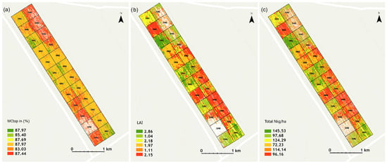
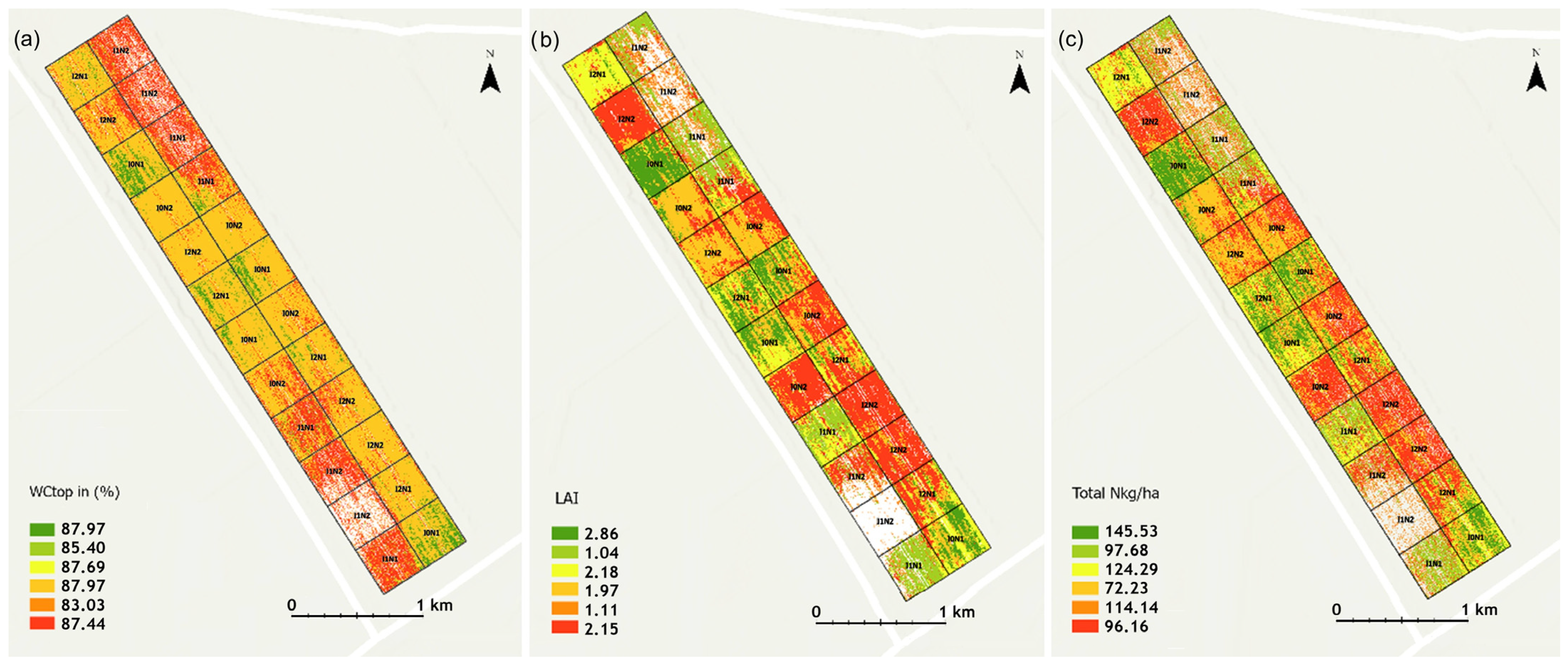
When comparing the classifiers (Table 2; the first three rows for class comparison), U-Net outperformed, achieving the best accuracy across treatments and reliably detecting N, water and LAI subtle variations (Table A2 and Table A3 in the Appendix A). It achieves about twice the accuracy in the mixed class group compared to the ML classifiers and nearly four times that of unsupervised classifier. The classification results spatially for crop N, LAI and water status are shown on Figure 6.
Figure 6.
Maps of (a) water status (WCrop), (b) leaf area index (LAI) and (c) nitrogen (Total N) for mid-season potato growth in the field experiments predicted from UAV multispectral data and U-Net model using G-RE-NIR bands as input.
3.5. Confirmation of Results at Another Date
The same classifiers were applied on data from the same year, field and crop but 10 days later, i.e., 8 August 2018. This situation is typical in precision agriculture to optimize water and/or N application rate (time and place) to match crop demands. The results (Table 4) show that all four classifiers reflected comparable pattern and magnitude of the classification accuracy as the earlier results (Table 2). Band combinations with the highest accuracy were the same, Green-RedEdge and near-infrared, and the classifier with the highest accuracy was U-Net, followed by SVM, RF and K-means. U-Net outperformed the other classifiers with more accurate borders and greater overall accuracy. SVM and RF also showed strong treatment separation with low misclassification, especially in two- and three-class settings. K-means showed more distributed class patches and higher border noise. This consistency across dates demonstrates dependability and durability of ML and deep learning models for properly categorizing crop water and N status and LAI (also see Table A2 and Table A3 in the Appendix A).
Table 4.
Classification accuracy (%, from low/red colour to high/blue colour) of unsupervised (USC; K-means), supervised machine learning (Support Vector Machine, SVM, Random Forest, RF) and deep learning (U-Net) for mid-season nitrogen status of potato. The results are from imagery obtained on 8 August 2018-10 days later than the original imagery to test robustness of the classifiers. Accuracy values for pooled treatments (N, I and N × I) were calculated according to Equation (2), while treatment-specific accuracy values were calculated according to Equation (3). Classes refer to treatment labels in Table 1. RGB, G, RE and Nir are true-color, green, red edge and near-infrared bands of the camera, respectively.
4. Discussion
Previous multispectral UAV studies have struggled to separately assess N and water status because water is primarily expressed in the atmospherically noisy shortwave infrared while N appears in both visible and shortwave infrared, making algorithms optimized for one resource to underperform for the other [35,36]. Our systematic comparison of ML and deep learning, however, identified U-Net as highly promising for detecting individual and co-occurring deficits.
Blekanov et al. [18] used U-Net for cereal N status quantification with multispectral UAV data and found RedEdge band negatively impacted segmentation, opposite to our study where RedEdge improved performance (e.g., NIR/edge and NIR/edge/green; Table 2 and Table 4). RedEdge inclusion in deep learning may be crop-specific. Colligan et al. [37] applied U-Net to Landsat multispectral satellite imagery over Montana, achieving high accuracy for irrigated pixels without extensive feature engineering.
Other studies using UAV, field, or satellite data reported satisfactory SVM and RF accuracies but focused on only N [38,39,40] or only water status [41]. For water status, Mpakairi et al. [41] used Sentinel-2 and found 71% deep learning model accuracy at national scale in South Africa; our UAV results showed 50–80% U-Net accuracy depended on bands and N × I interaction and it was the sole algorithm capturing water status under no irrigation (I2; 45–72%, Table 2, 43–70%, Table 4), highlighting its value for deficit irrigation. During the 2018 drought, non-irrigated treatment (I2) caused severe canopy wilting, and U-Net correctly reported many “empty pixels” (Figure 6) [3]. All classifiers improved accuracy with fewer classes, but this reduced ability to describe complex and subtle spatial variability from interacting N and water deficiencies. SVM and RF successfully identified classes I2N1 and I1N2 (Table 2; Figure 6), albeit with limitations. At fine spatial scales, canopy pixels with similar water/N status from different treatments were classified. Green, RedEdge, and NIR band combination yielded highest accuracy, closely followed by the all-bands combination (Table 2 and Table 4), suggesting that these bands are effective to detect potato canopy N and water levels.
K-means was selected as an unsupervised baseline to assess the inherent separability of the spectral data without prior labeling, SVM and RF were chosen as representative conventional supervised methods due to their proven robustness with high-dimensional multispectral features, and U-Net was adopted as the deep learning architecture to exploit its encoder–decoder structure for capturing spatial context and hierarchical features essential for pixel-wise segmentation of subtle stress patterns. While previous work tested ML regressor (RF) to predict N for the same crop and field, identifying RF as the best performer [2], our study goes one important step further by comparing several ML models against a deep learning model (U-Net). The U-Net model significantly outperformed unsupervised and supervised ML classifiers, achieving segmentation accuracies of 70% (six mixed N × I classes), 93% (irrigation classes), and 85% (nitrogen classes). Its encoder–decoder structure captures spatial feature hierarchies, as confirmed by training/validation loss and accuracy metrics. For the complex class I2N1, i.e., no irrigation, variable fertilization under drought conditions where N uptake is hampered by water stress [2,3], precision was 0.76, recall 0.85, and F1-score 0.80. Class I0N2 yielded an F1-score of 0.76. Visual comparison of predicted and actual masks (Figure 6) supports these quantitative results. Ma et al. [7] in their meta-analysis found unexplored potential of deep learning models in agricultural remote sensing; our study demonstrates that potential for describing interacting crop N and water status. To train the neural network, we generated synthetic data because initial training with original data yielded <50% accuracy. Deep learning models require very large training data volumes, which poses a drawback for operationalizing the algorithm within an agricultural cybernetics framework unless super-computing is available. Future studies should complement our single-training protocol with repeated independent training sessions using different random seeds and cross-validation strategies to quantify the variance of deep learning performance in the context of subtle N-water co-limitation detection. Cross-validation should account for the spatial structure of the experimental design, for instance, by training the model on three of the four replicate plots and validating on the completely held-out fourth replicate, in order to ensure that high classification accuracy reflects spectral-physiological relationships rather than the model inadvertently learning the spatial layout or row patterns of the treatment plots. Additionally, regressing the continuous physiological values (kg N ha−1 and %W) instead of classifying discrete categories of management treatments based on these physiological values should also be tested. Such an approach would unequivocally confirm the model’s utility in detecting actual co-limitation signals independent of nominal treatment labels, providing stronger evidence for operational fertigation decisions. Also, the absence of multi-site, multi-crop, or multi-season replication sets the U-Net superiority conditional on this specific dataset, although the radiometric principles remain. Future work could extend this comparison across broader spatio-temporal gradients to robustly validate the adoption of deep learning for operational N and irrigation management in potato or other crops.
The unsupervised classification provided a baseline for comparison in this study, with accuracy levels of 41% for the N classes, 36% for the I classes, and 23% for N × I classes. Many learning problems in agriculture require handling high-dimensional datasets with a relatively small number of classes, for instance variation in a single factor. For N, the results show some potential of the K-means (Table 2 and Table 4), though the accuracy was low for precision N or water management needs. Unsupervised classifiers have been successfully deployed for spatial and temporal discrimination of crop types, e.g., [42]; however, biophysical properties such as N and water contents require some degree of human interaction. In contrast to task-oriented supervised learning, unsupervised learning is data-oriented, and the subtle spatial variation might be too detailed for identifying accurate treatment class patterns. For main clustering, however, we deem the K-means useful [43].
5. Conclusions
Supervised ML (SVM, RF) and the U-Net deep learning model outperformed the unsupervised K-means classifier for the complex task of detecting crop N and water status under different N fertilization and irrigation treatments and under field conditions. U-Net further excelled at separating subtle spatial and temporal variation from different irrigation and N fertilization levels, achieving 65–99% accuracy for N classes, 84–99% for I classes, and 41–82% for N × I factorial classes, with variation due to input data, cleaner boundaries and less noise. In comparison, SVM reached 53–87, 66–86, and 32–66%, RF reached 61–96, 70–81, and 33–65%, and K-means only 47–57, 9–65, and 8–34%, respectively. U-Net also showed more balanced accuracy across treatments within the same class group. SVM and RF remain good alternatives when computational resources are limited. Despite single-season single crop nature of the study, the results clearly show the potential of deep learning for detangling crop N and water status under resource co-limitation under real field conditions. Future research should integrate soil moisture or weather data and explore other deep learning architectures. The U-Net’s superior ability to simultaneously map crop N and water status under variable field conditions makes it a highly promising tool for applied fertigation decisions, enabling precise, site-specific recommendations of when and where to apply N and irrigation together.
Author Contributions
Conceptualization, C.F., S.W. and K.M.; methodology, C.F., S.W. and K.M.; software, C.F., S.W. and K.M.; validation, B.M., X.Y., S.Z., S.N. and J.P.; formal analysis, C.F.; investigation, C.F., S.W. and K.M.; resources, C.K. and K.M.; data curation, C.K. and K.M.; writing—original draft preparation, C.F. and K.M.; writing—review and editing, S.W., B.M., X.Y., S.Z., S.N., J.P. and C.K.; visualization, C.F., B.M. and K.M.; supervision, S.W., C.K. and K.M.; project administration, C.K. and K.M.; funding acquisition, C.K. and K.M. All authors have read and agreed to the published version of the manuscript.
Funding
This research received no external funding.
Institutional Review Board Statement
Not applicable.
Informed Consent Statement
Not applicable.
Data Availability Statement
The data presented in this study are available on request from the corresponding author due to large size exceeding the storage limits of standard public repositories.
Acknowledgments
The data for this study were obtained through the Innovation Fund Denmark ERA-NET Co-fund Waterworks 2015 project ‘POTENTIAL’-Variable rate irrigation and nitrogen fertilization in potato; Engage the spatial variation. Corresponding author also thanks the Chinese Academy of Sciences President International Fellowship Initiative (PIFI) grant no. 2026PVB0038.
Conflicts of Interest
Author Blagoja Mukanov was employed by the company AgFutura. The remaining authors declare that the research was conducted in the absence of any commercial or financial relationships that could be construed as a potential conflict of interest.
Abbreviations
The following abbreviations are used in this manuscript:
| I | Irrigation |
| LAI | Leaf Area Index |
| ML | Machine learning |
| N | Nitrogen |
| RF | Random Forest |
| RGB | Red Green Blue (true color) |
| SVM | Support Vector Machine |
| UAV | Unmanned Aerial Vehicle |
Appendix A
Figure A1.
Accuracy of unsupervised classifier (K-means) for mid-season water and nitrogen status of potato using thresholds 0.45 vs. 0.3 to mask soil. Classes refer to treatment labels in Table 1.
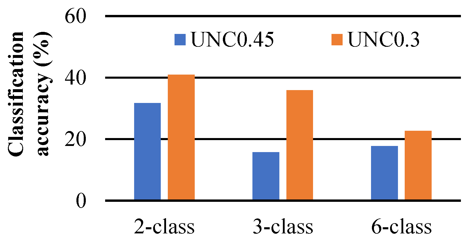
Table A1.
Classification accuracy (%, from low/red colour to high/blue colour) of unsupervised (USC; K-means) for mid-season nitrogen status of potato using two different thresholds to discriminate soil. Accuracy values for pooled treatments (N, I and N × I) were calculated according to Equation (2), while treatment-specific accuracy values were calculated according to Equation (3). Classes refer to treatment labels in Table 1. RGB, G, RE and Nir are true-color, green, red edge and near-infrared bands of the camera, respectively.
Table A2.
Classification accuracy (%, from low/red colour to high/blue colour) of unsupervised (USC; K-means), supervised machine learning (Support Vector Machine, SVM, Random Forest, RF) and deep learning (U-Net) for mid-season leaf area index of potato. Accuracy values for pooled treatments (N, I) were calculated according to Equation (2), while treatment-specific accuracy values were calculated according to Equation (3). Classes refer to treatment labels in Table 1. RGB, G, RE and Nir are true-color, green, red edge and near-infrared bands of the camera, respectively.
Table A3.
Classification accuracy (%, from low/red colour to high/blue colour) of unsupervised (USC; K-means), supervised machine learning (Support Vector Machine, SVM, Random Forest, RF) and deep learning (U-Net) for mid-season crop water status of potato. Accuracy values for pooled treatments (N, I) were calculated according to Equation (2), while treatment-specific accuracy values were calculated according to Equation (3). Classes refer to treatment labels in Table 1. RGB, G, RE and Nir are true-color, green, red edge and near-infrared bands of the camera, respectively.
References
- Manevski, K.; Andersen, M.N. Field-Level Irrigation; Oxford University Press: Oxford, UK, 2024. [Google Scholar] [CrossRef] [Scilit]
- Peng, J.; Manevski, K.; Kørup, K.; Larsen, R.; Andersen, M.N. Random forest regression results in accurate assessment of potato nitrogen status based on multispectral data from different platforms and the critical concentration approach. Field Crops Res. 2021, 268, 108158. [Google Scholar] [CrossRef] [Scilit]
- Peng, J.; Nieto, H.; Neumann Andersen, M.; Kørup, K.; Larsen, R.; Morel, J.; Parsons, D.; Zhou, Z.; Manevski, K. Accurate estimates of land surface energy fluxes and irrigation requirements from UAV-based thermal and multispectral sensors. ISPRS J. Photogramm. Remote Sens. 2023, 198, 238–254. [Google Scholar] [CrossRef] [Scilit]
- Attri, I.; Awasthi, L.K.; Sharma, T.P.; Rathee, P. A review of deep learning techniques used in agriculture. Ecol. Inf. 2023, 77, 102217. [Google Scholar] [CrossRef] [Scilit]
- Artley, B. Unsupervised Learning: K-Means Clustering—The Fastest and Most Intuitive Unsupervised Clustering Algorithm. Available online: https://towardsdatascience.com/unsupervised-learning-k-means-clustering-27416b95af27 (accessed on 20 May 2025).
- Sharma, A.; Jain, A.; Gupta, P.; Chowdary, V. Machine Learning Applications for Precision Agriculture: A Comprehensive Review. IEEE Access 2021, 9, 4843–4873. [Google Scholar] [CrossRef] [Scilit]
- Ma, L.; Liu, Y.; Zhang, X.; Ye, Y.; Yin, G.; Johnson, B.A. Deep learning in remote sensing applications: A meta-analysis and review. ISPRS J. Photogramm. Remote Sens. 2019, 152, 166–177. [Google Scholar] [CrossRef] [Scilit]
- Mountrakis, G.; Im, J.; Ogole, C. Support vector machines in remote sensing: A review. ISPRS J. Photogramm. Remote Sens. 2011, 66, 247–259. [Google Scholar] [CrossRef] [Scilit]
- Belgiu, M.; Dragut, L. Random forest in remote sensing: A review of applications and future directions. ISPRS J. Photogramm. Remote Sens. 2016, 114, 24–31. [Google Scholar] [CrossRef] [Scilit]
- Li, T.; Johansen, K.; McCabe, M.F. A machine learning approach for identifying and delineating agricultural fields and their multi-temporal dynamics using three decades of Landsat data. ISPRS J. Photogramm. Remote Sens. 2022, 186, 83–101. [Google Scholar] [CrossRef] [Scilit]
- Darwin, B.; Dharmaraj, P.; Prince, S.; Popescu, D.E.; Hemanth, D.J. Recognition of Bloom/Yield in Crop Images Using Deep Learning Models for Smart Agriculture: A Review. Agronomy 2021, 11, 646. [Google Scholar] [CrossRef] [Scilit]
- Yang, H.B.; Li, F.; Wang, W.; Yu, K. Estimating Above-Ground Biomass of Potato Using Random Forest and Optimized Hyperspectral Indices. Remote Sens. 2021, 13, 2339. [Google Scholar] [CrossRef] [Scilit]
- Shen, Y.L.; Mercatoris, B.; Cao, Z.; Kwan, P.; Guo, L.F.; Yao, H.X.; Cheng, Q. Improving Wheat Yield Prediction Accuracy Using LSTM-RF Framework Based on UAV Thermal Infrared and Multispectral Imagery. Agriculture 2022, 12, 892. [Google Scholar] [CrossRef] [Scilit]
- Yang, H.; Yin, H.; Li, F.; Hu, Y.; Yu, K. Machine learning models fed with optimized spectral indices to advance crop nitrogen monitoring. Field Crops Res. 2023, 293, 108844. [Google Scholar] [CrossRef] [Scilit]
- Peng, Y.; He, M.; Zheng, Z.; He, Y. Enhanced Neural Network for Rapid Identification of Crop Water and Nitrogen Content Using Multispectral Imaging. Agronomy 2023, 13, 2464. [Google Scholar] [CrossRef] [Scilit]
- Cossani, C.M.; Sadras, V.O. Chapter Six—Water–Nitrogen Colimitation in Grain Crops. In Advances in Agronomy; Sparks, D.L., Ed.; Academic Press: New York, NY, USA, 2018; Volume 150, pp. 231–274. [Google Scholar]
- Elbasi, E.; Zaki, C.; Topcu, A.E.; Abdelbaki, W.; Zreikat, A.I.; Cina, E.; Shdefat, A.; Saker, L. Crop Prediction Model Using Machine Learning Algorithms. Appl. Sci. 2023, 13, 9288. [Google Scholar] [CrossRef] [Scilit]
- Blekanov, I.; Molin, A.; Zhang, D.; Mitrofanov, E.; Mitrofanova, O.; Li, Y. Monitoring of grain crops nitrogen status from uav multispectral images coupled with deep learning approaches. Comput. Electron. Agric. 2023, 212, 108047. [Google Scholar] [CrossRef] [Scilit]
- LeCun, Y.; Bengio, Y.; Hinton, G. Deep learning. Nature 2015, 521, 436–444. [Google Scholar] [CrossRef] [Scilit] [PubMed]
- Egger, J.; Gsaxner, C.; Pepe, A.; Pomykala, K.L.; Jonske, F.; Kurz, M.; Li, J.; Kleesiek, J. Medical deep learning—A systematic meta-review. Comput. Methods Programs Biomed. 2022, 221, 106874. [Google Scholar] [CrossRef] [Scilit] [PubMed]
- Esteva, A.; Robicquet, A.; Ramsundar, B.; Kuleshov, V.; DePristo, M.; Chou, K.; Cui, C.; Corrado, G.; Thrun, S.; Dean, J. A guide to deep learning in healthcare. Nat. Med. 2019, 25, 24–29. [Google Scholar] [CrossRef] [Scilit] [PubMed]
- Rai, N.; Zhang, Y.; Ram, B.G.; Schumacher, L.; Yellavajjala, R.K.; Bajwa, S.; Sun, X. Applications of deep learning in precision weed management: A review. Comput. Electron. Agric. 2023, 206, 107698. [Google Scholar] [CrossRef] [Scilit]
- Chen, Y.; Huang, Y.; Zhang, Z.; Wang, Z.; Liu, B.; Liu, C.; Huang, C.; Dong, S.; Pu, X.; Wan, F.; et al. Plant image recognition with deep learning: A review. Comput. Electron. Agric. 2023, 212, 108072. [Google Scholar] [CrossRef] [Scilit]
- Sanaeifar, A.; Guindo, M.L.; Bakhshipour, A.; Fazayeli, H.; Li, X.; Yang, C. Advancing precision agriculture: The potential of deep learning for cereal plant head detection. Comput. Electron. Agric. 2023, 209, 107875. [Google Scholar] [CrossRef] [Scilit]
- Dale, D.S.; Liang, L.; Zhong, L.; Reba, M.L.; Runkle, B.R.K. Dataset for Deep learning solutions for mapping contour levee rice production systems from very high resolution imagery. Comput. Electron. Agric. 2023, 211, 107954. [Google Scholar] [CrossRef] [Scilit]
- Raei, E.; Akbari Asanjan, A.; Nikoo, M.R.; Sadegh, M.; Pourshahabi, S.; Adamowski, J.F. A deep learning image segmentation model for agricultural irrigation system classification. Comput. Electron. Agric. 2022, 198, 106977. [Google Scholar] [CrossRef] [Scilit]
- Pancorbo, J.L.; Camino, C.; Alonso-Ayuso, M.; Raya-Sereno, M.D.; Gonzalez-Fernandez, I.; Gabriel, J.L.; Zarco-Tejada, P.J.; Quemada, M. Simultaneous assessment of nitrogen and water status in winter wheat using hyperspectral and thermal sensors. Eur. J. Agron. 2021, 127, 126287. [Google Scholar] [CrossRef] [Scilit]
- Peng, J.; Manevski, K.; Kørup, K.; Larsen, R.; Zhou, Z.; Andersen, M.N. Environmental constraints to net primary productivity at northern latitudes: A study across scales of radiation interception and biomass production of potato. Int. J. Appl. Earth Obs. 2021, 94, 102232. [Google Scholar] [CrossRef] [Scilit]
- Zhou, Z.; Plauborg, F.; Thomsen, A.G.; Andersen, M.N. A RVI/LAI-reference curve to detect N stress and guide N fertigation using combined information from spectral reflectance and leaf area measurements in potato. Eur. J. Agron. 2017, 87, 1–7. [Google Scholar] [CrossRef] [Scilit]
- Boiarskii, B.; Hasegawa, H. Comparison of NDVI and NDRE Indices to Detect Differences in Vegetation and Chlorophyll Content. J. Mech. Contin. Math. Sci. 2019, 4, 20–29. [Google Scholar] [CrossRef] [Scilit]
- Ronneberger, O.; Fischer, P.; Brox, T. U-Net: Convolutional Networks for Biomedical Image Segmentation. In Proceedings of the International Conference on Medical Image Computing and Computer-Assisted Intervention (MICCAI), Munich, Germany, 5–9 October 2015; pp. 234–241. [Google Scholar] [CrossRef] [Scilit]
- Farahani, A.; Mohseni, H. Medical image segmentation using customized U-Net with adaptive activation functions. Neural Comput. Appl. 2021, 33, 6307–6323. [Google Scholar] [CrossRef] [Scilit]
- Anwar, S.M.; Majid, M.; Qayyum, A.; Awais, M.; Alnowami, M.; Khan, M.K. Medical Image Analysis using Convolutional Neural Networks: A Review. J. Med. Syst. 2018, 42, 226. [Google Scholar] [CrossRef] [Scilit] [PubMed]
- Zhang, S.W.; Zhang, C.L. Modified U-Net for plant diseased leaf image segmentation. Comput. Electron. Agric. 2023, 204, 107511. [Google Scholar] [CrossRef] [Scilit]
- Curran, P.J. Imaging Spectrometry. Prog. Phys. Geogr. 1994, 18, 247–266. [Google Scholar] [CrossRef] [Scilit]
- Mutanga, O.; Skidmore, A.K. Red edge shift and biochemical content in grass canopies. ISPRS J. Photogramm. Remote Sens. 2007, 62, 34–42. [Google Scholar] [CrossRef] [Scilit]
- Colligan, T.; Ketchum, D.; Brinkerhoff, D.; Maneta, M. A Deep Learning Approach to Mapping Irrigation Using Landsat: IrrMapper U-Net. IEEE Trans. Geosci. Remote 2022, 60, 4411611. [Google Scholar] [CrossRef] [Scilit]
- Gao, J.; Liang, T.; Liu, J.; Yin, J.; Ge, J.; Hou, M.; Feng, Q.; Wu, C.; Xie, H. Potential of hyperspectral data and machine learning algorithms to estimate the forage carbon-nitrogen ratio in an alpine grassland ecosystem of the Tibetan Plateau. ISPRS J. Photogramm. Remote Sens. 2020, 163, 362–374. [Google Scholar] [CrossRef] [Scilit]
- Li, Y.; Miao, Y.; Zhang, J.; Cammarano, D.; Li, S.; Liu, X.; Tian, Y.; Zhu, Y.; Cao, W.; Cao, Q. Improving Estimation of Winter Wheat Nitrogen Status Using Random Forest by Integrating Multi-Source Data Across Different Agro-Ecological Zones. Front. Plant Sci. 2022, 13, 890892. [Google Scholar] [CrossRef] [Scilit] [PubMed]
- Zha, H.N.; Miao, Y.X.; Wang, T.T.; Li, Y.; Zhang, J.; Sun, W.C.; Feng, Z.Q.; Kusnierek, K. Improving Unmanned Aerial Vehicle Remote Sensing-Based Rice Nitrogen Nutrition Index Prediction with Machine Learning. Remote Sens. 2020, 12, 215. [Google Scholar] [CrossRef] [Scilit]
- Mpakairi, K.S.; Dube, T.; Sibanda, M.; Mutanga, O. Fine-scale characterization of irrigated and rainfed croplands at national scale using multi-source data, random forest, and deep learning algorithms. ISPRS J. Photogramm. Remote Sens. 2023, 204, 117–130. [Google Scholar] [CrossRef] [Scilit]
- Wang, Y.; Feng, L.; Zhang, Z.; Tian, F. An unsupervised domain adaptation deep learning method for spatial and temporal transferable crop type mapping using Sentinel-2 imagery. ISPRS J. Photogramm. Remote Sens. 2023, 199, 102–117. [Google Scholar] [CrossRef] [Scilit]
- Ennaji, O.; Vergütz, L.; El Allali, A. Machine learning in nutrient management: A review. Artif. Intell. Agric. 2023, 9, 1–11. [Google Scholar] [CrossRef] [Scilit]

Disclaimer/Publisher’s Note: The statements, opinions and data contained in all publications are solely those of the individual author(s) and contributor(s) and not of MDPI and/or the editor(s). MDPI and/or the editor(s) disclaim responsibility for any injury to people or property resulting from any ideas, methods, instructions or products referred to in the content. |
© 2026 by the authors. Licensee MDPI, Basel, Switzerland. This article is an open access article distributed under the terms and conditions of the Creative Commons Attribution (CC BY) license.