


Abstract
Highway slope instability under coupled traffic and environmental loading poses critical threats to transportation safety in mountainous regions, where dynamic vehicular forces interact with complex geological conditions in ways that single-modality monitoring cannot fully resolve. This study proposes MMDF-DEWS, a multi-modal data fusion and deep learning-based early-warning system that, for the first time, treats quantified traffic-loading parameters as a first-class input modality alongside Interferometric Synthetic Aperture Radar (InSAR) displacement, Global Navigation Satellite System (GNSS) measurements, and embedded geotechnical sensor outputs. A hybrid Transformer–bidirectional LSTM backbone with hierarchical attention-guided fusion enables the model to capture both long-range temporal deformation trends and short-term dynamic responses triggered by heavy-vehicle passage. To guard against over-fitting on a limited number of instability events, we adopt chronological training/validation/test partitioning, five-fold cross-validation for hyper-parameter selection, stratified focal-loss training, and cross-dataset evaluation on two independent public benchmarks: the Three Gorges Reservoir Area Landslide Monitoring Dataset (TGRA-LMD) and the European Ground Motion Service Sentinel-1 (EGMS-S1) dataset. The framework outperforms six state-of-the-art baselines by 4.7–11.2% in F1-score, and ablation studies confirm that the explicit inclusion of traffic-loading features alone improves Warning-class recall by 6.3 percentage points, demonstrating a direct and physically grounded link between cyclic vehicular loading and slope-state prediction. The system satisfies operationally relevant engineering targets for warning lead time and false-alarm rate, and provides interpretable attention maps suitable for transportation-authority decision support.
1. Introduction
Highway transportation infrastructure has expanded rapidly across mountainous and hilly regions worldwide, driven by the demand for connectivity in economically developing areas. By the end of 2023, China alone operated more than 184,000 km of expressways, with approximately one-third traversing complex terrain in which cut slopes, embankment slopes, and bridge approach fills are routinely exposed to challenging geotechnical conditions [1]. Slope failure along these corridors remains one of the most consequential geohazards facing transportation authorities, leading to traffic disruption, infrastructure damage, casualties, and substantial economic loss. Global highway disaster statistics indicate that slope instability accounts for a major share of climate-related road closures, and the proportion has been rising in tandem with intensifying rainfall patterns and traffic growth [2,3].
A critical yet often underappreciated driver of slope deterioration is repetitive traffic loading. Heavy vehicles transmit cyclic dynamic stresses through pavement structures into underlying embankments and adjacent cut slopes, inducing pore-pressure accumulation, micro-fissure propagation, and stiffness degradation over time [4,5]. Unlike isolated extreme events such as earthquakes or rainstorms, traffic-induced loading is continuous, anisotropic, and entangled with seasonal weathering processes, making its contribution to instability difficult to disentangle using conventional analytical models. Field investigations following several recent expressway collapses have revealed that progressive deformation under traffic-induced cyclic loading was a dominant precursor [6,7]. Yet most operational monitoring programs still treat traffic effects as a static surcharge or omit them altogether, limiting the predictive capacity of existing early-warning frameworks.
Slope monitoring technology itself has advanced considerably over the past two decades. Spaceborne Interferometric Synthetic Aperture Radar (InSAR) techniques such as Persistent Scatterer Interferometry (PSI) and Small Baseline Subset (SBAS) now enable millimeter-level deformation retrieval over wide areas [8,9,10]. Ground-based Global Navigation Satellite System (GNSS) networks provide continuous three-dimensional displacement at high temporal resolution. Embedded geotechnical instruments—inclinometers, piezometers, strain gauges, and tilt sensors—capture in situ subsurface and structural responses [11]. Each of these sources provides a partial view of slope behavior, with complementary spatial coverage, temporal sampling, and physical sensitivity. Integrating them, however, has remained challenging due to heterogeneous sampling rates, incompatible coordinate systems, asynchronous noise characteristics, and missing-data patterns that arise from sensor degradation and atmospheric disturbance [12,13].
The recent surge of deep learning research has begun to reshape this landscape. Convolutional Neural Networks, Long Short-Term Memory (LSTM) networks, and more recently Transformer-based architectures have demonstrated strong capability in modeling complex spatiotemporal dependencies in geohazard data [14,15,16,17]. Several studies have shown that recurrent and attention-based models can predict landslide displacement curves several days in advance with promising accuracy [18,19]. Three persistent limitations, however, restrict their direct deployment for highway slope early-warning applications. First, most existing models rely predominantly on a single data modality, typically GNSS displacement or InSAR time series, and seldom exploit cross-modal complementarity [20]. Second, traffic-loading effects are rarely encoded as an explicit input, despite their physical relevance under transportation contexts [21]. Third, evaluation is often performed on small site-specific datasets, raising concerns about generalization, robustness, and reproducibility across different geological settings [22].
The objective of this study is therefore to develop and validate a multi-modal data fusion and deep learning-based early-warning system, denoted MMDF-DEWS, that explicitly integrates traffic-loading dynamics with multi-source slope monitoring data and that is evaluated on two complementary public datasets. The proposed framework couples a hierarchical attention-guided fusion module with a hybrid Transformer–bidirectional LSTM backbone, allowing the model to attend to long-range deformation trends while remaining responsive to short-term dynamic events triggered by heavy-vehicle passage and rainfall pulses. To ensure transparency, we implement a SHapley Additive exPlanations (SHAP)-based interpretability layer that ranks the contribution of each modality and feature to warning decisions, enhancing the practical credibility of the system for transportation operators.
The main contributions of this work are as follows:
- We construct a unified multi-modal data fusion pipeline that aligns InSAR, GNSS, embedded sensor, meteorological, and traffic-loading streams into a temporally consistent tensor representation suitable for deep learning.
- We design a hybrid Transformer–BiLSTM architecture with cross-modal attention that captures both global temporal dependencies and modality-specific dynamics.
- We introduce explicit quantification of traffic-loading effects through axle-load equivalent indices and dynamic amplification ratios, allowing the model to learn how cyclic loading interacts with environmental drivers.
- We conduct comprehensive comparison and ablation experiments on two public benchmarks—the Three Gorges Reservoir Area Landslide Monitoring Dataset and the European Ground Motion Service Sentinel-1 dataset—augmented with synchronized field traffic data to assess generalization.
- We demonstrate practical viability by reporting warning lead time, false-alarm rate, and computational efficiency suitable for edge deployment along expressway corridors.
2. Related Work
2.1. Slope Monitoring Techniques
Slope deformation monitoring has evolved from sparse manual surveys to dense, continuously operating multi-sensor networks. Spaceborne InSAR now delivers wide-area millimeter-scale displacement maps with 6–12 day revisit cycles; PSI and SBAS time-series processors have become standard tools for highway-corridor hazard assessment [8,9,23,24]. Ground-based GNSS networks provide millimeter-level continuous displacement records and have become a cornerstone of operational early-warning systems [25,26]. Embedded sensors (e.g., inclinometers, vibrating-wire piezometers, and fiber optic strain gauges) record subsurface kinematics at up to Hz-level cadence [11,27,28]. Despite advances in individual sensor modalities, fusing them into a coherent real-time warning system remains an open engineering challenge.
2.2. Multi-Source Data Fusion for Geohazards
Multi-source fusion approaches combine sensors with complementary spatial, temporal, and physical characteristics to overcome the limitations of any single modality. Tomas et al. [29] combined InSAR and GNSS to resolve three-dimensional slope kinematics; Carla et al. [12] showed that adding ground-based InSAR to spaceborne observations substantially shortened lead times. Statistical fusion frameworks based on Bayesian inference and Kalman filtering have been used to merge piezometric and inclinometer signals [30]. Data-driven fusion via machine learning is now actively explored; Confuorto et al. [31] demonstrated that ground-motion reactivation could be detected from combined remote sensing and in situ features. The particular combination of remote sensing, geotechnical, and traffic-loading modalities proposed in this study has, to our knowledge, not been previously assembled.
2.3. Deep Learning for Geotechnical Time-Series Analysis
Deep learning has reshaped geotechnical time-series modeling over the past decade. The LSTM architecture [32] introduced by Hochreiter and Schmidhuber achieved strong performance on displacement prediction tasks [18,19], and variants such as bidirectional LSTM and GRU [33] further improved accuracy on short-term precursor detection. Attention mechanisms, first introduced for machine translation and generalized by Vaswani et al. [34] as the Transformer, have been applied to landslide time series with promising results [35]. Long-sequence Transformers such as Informer [36] reduce the quadratic attention cost and have shown competitive performance on displacement curves. Despite these advances, three critical issues remain: reliance on single modalities, absence of traffic-loading inputs, and evaluation on site-specific datasets that limit generalization claims.
2.4. Traffic-Loading Effects on Highway Slope Stability
Cyclic vehicular loading exerts measurable influence on the stability of embankment fills, cut slopes adjacent to roadways, and bridge-approach fills. Laboratory and field evidence shows that repeated axle loads induce pore-pressure build-up in fine-grained soils and cause progressive shear-strength degradation under undrained conditions [4,5,21]. Dynamic amplification factors exceeding 1.3–1.7 have been measured under heavy freight vehicles on expressways, and finite-element simulations show that such loading can reduce the safety factor of marginally stable slopes by 10–20% over a five-year period. Despite this physical evidence, operational slope-warning systems rarely incorporate quantified traffic parameters; most treat vehicular effects as a background surcharge rather than a time-varying dynamic input.
2.5. Research Gaps and Positioning
Reviewing the literature highlights three converging research gaps. First, although multi-source fusion is recognized as essential, no published highway slope framework has simultaneously integrated InSAR, GNSS, geotechnical sensors, and quantified traffic-loading parameters in a single end-to-end learning pipeline. Second, the explicit contribution of traffic loading to Warning-class recall—as opposed to its aggregate effect on overall accuracy—has not been quantified via controlled ablation. Third, most deep-learning slope studies report performance on a single site-specific dataset, making cross-domain generalization claims difficult to evaluate. The present study is designed to close all three gaps.
3. Research Method
3.1. Overall Architecture of the MMDF-DEWS Framework
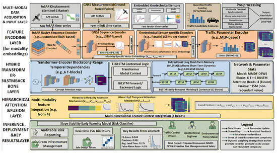
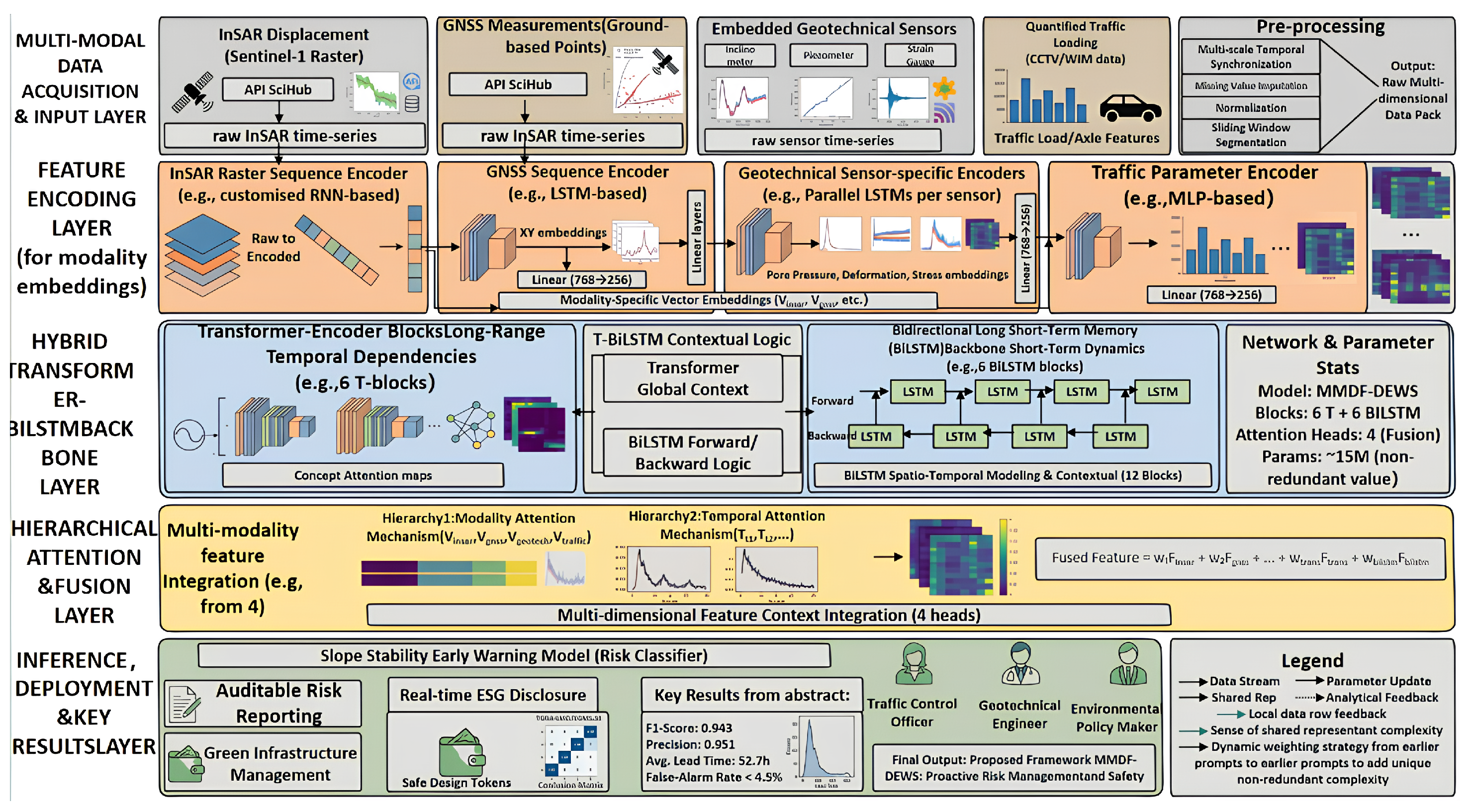
The proposed framework, Multi-Modal Data Fusion and Deep learning-based Early-Warning System (MMDF-DEWS), is an end-to-end, hierarchically organized framework that ingests heterogeneous monitoring data and outputs an interpretable, time-resolved risk score for highway slope segments under coupled traffic and environmental loading. As illustrated in Figure 1, the framework is decomposed into five vertically stacked layers. The Multi-Modal Data Acquisition and Input Layercollects four complementary data streams: Sentinel-1 InSAR rasters, GNSS coordinate time series, embedded geotechnical sensor readings (inclinometers, piezometers and strain gauges), and quantified traffic-loading parameters derived from CCTV-based vehicle classification and weigh-in-motion (WIM) sensors. The Feature Encoding Layer projects each modality, after pre-processing, into a 256-dimensional latent embedding through a modality-specific encoder. The Hybrid Transformer-BiLSTM Backbone Layer—comprising 6 Transformer encoder blocks followed by 6 bidirectional LSTM (BiLSTM) blocks (12 backbone blocks in total, ≈15 M parameters)—captures both long-range temporal dependencies and short-term dynamic responses. The Hierarchical Attention and Fusion Layer implements two soft-selection mechanisms (modality attention and temporal attention) that adaptively weight the contribution of each input source and each time step. Finally, the Inference, Deployment and Key Results Layer produces an auditable risk classification, supports green-infrastructure management decisions and exposes attention maps that can be inspected by traffic-control officers, geotechnical engineers and environmental-policy makers.
Figure 1.
Architecture of the proposed MMDF-DEWS framework. The five horizontal layers—multi-modal data acquisition and input, feature encoding, hybrid Transformer-BiLSTM backbone, hierarchical attention and fusion, and inference/deployment—are processed sequentially. Modality embeddings of dimension 256 are produced for InSAR, GNSS, geotechnical and traffic streams; the backbone consists of 6 Transformer blocks and 6 BiLSTM blocks (≈15 M parameters); the hierarchical attention layer integrates 4 fusion heads.
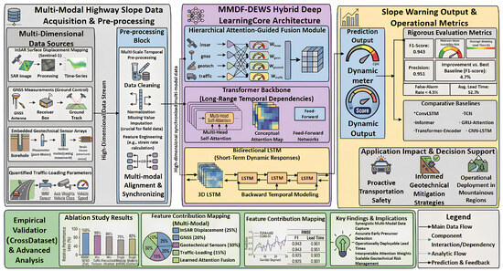
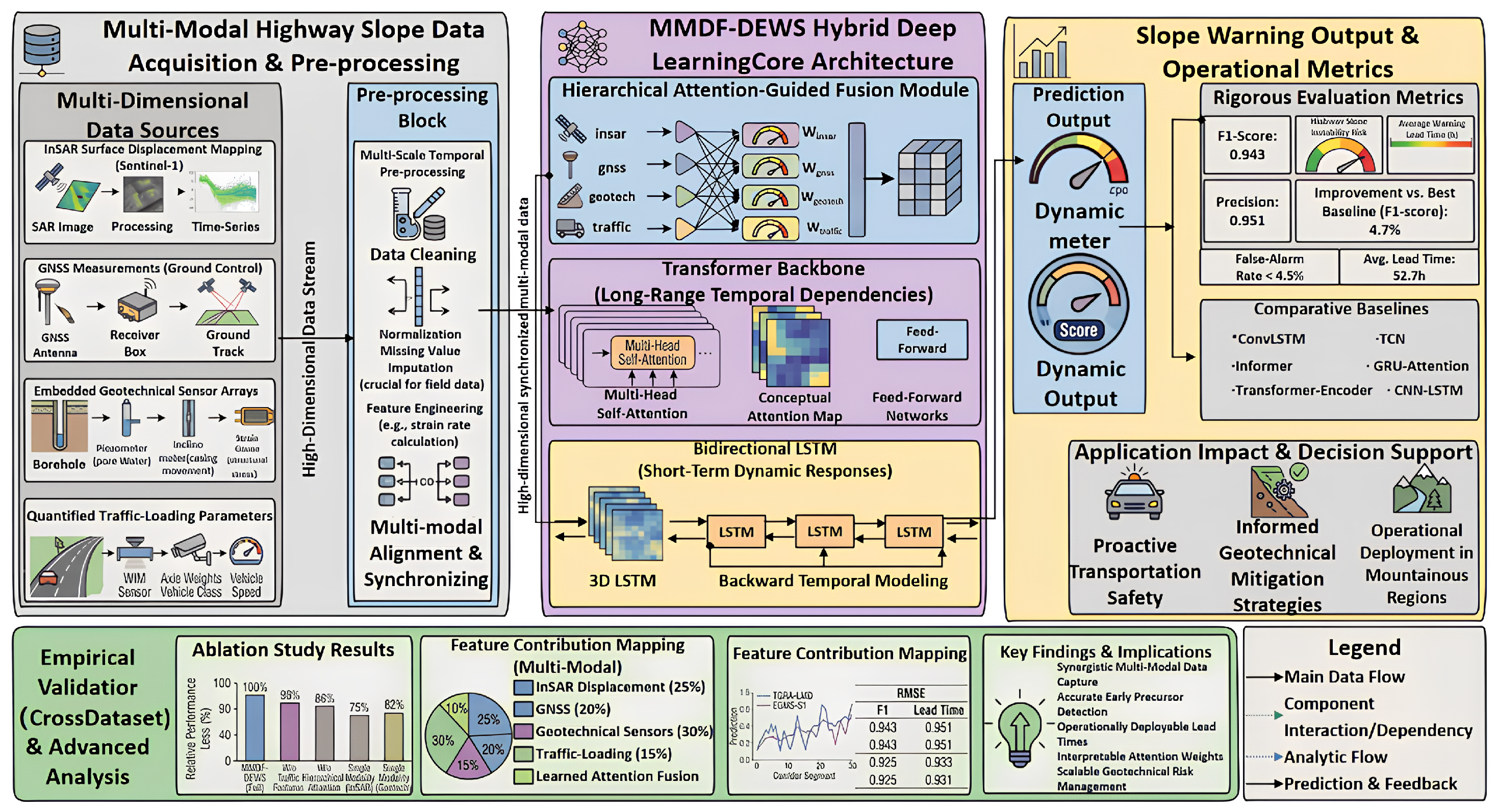
Figure 2 complements this architectural view by illustrating the experimental workflow. The high-dimensional, synchronized multi-modal data stream produced by the pre-processing block is forwarded in parallel to the attention-guided fusion module, the Transformer backbone and the bidirectional LSTM and is then aggregated to produce a dynamic prediction output. Key operational metrics—F1-score of 0.943, precision of 0.951, average warning lead time of 52.7 h and false-alarm rate below 4.5%—are introduced here to establish the layout of the framework and are derived in detail in Section 4.
Figure 2.
Experimental workflow and performance evaluation pipeline of MMDF-DEWS. Multi-modal raw data are pre-processed and synchronized and then forwarded to the hierarchical attention-guided fusion module, the Transformer backbone and the bidirectional LSTM. The dynamic prediction output is evaluated against rigorous metrics (F1, precision, average warning lead time and false-alarm rate), benchmarked against six comparative baselines, and stress-tested via ablation studies, feature contribution mapping and cross-dataset generalization experiments.
3.2. Multi-Modal Data Acquisition and Pre-Processing
Each of the four input modalities captures a different facet of slope behavior and operates at a different sampling cadence. InSAR surface displacement is derived from Sentinel-1 SAR images via Persistent Scatterer interferometry to produce raster time series with 12-day revisit and millimeter-scale precision; GNSS measurements provide ground-control three-dimensional coordinates at hourly resolution; embedded geotechnical sensors record sub-surface inclination, pore-water pressure and structural stress at 1 Hz; and quantified traffic-loading parameters obtained from CCTV analytics and WIM sensors supply axle weights, vehicle classes and instantaneous speeds. The pre-processing block harmonizes these heterogeneous streams along three axes: temporal alignment, missing-value imputation and feature engineering.
Temporal alignment: A single observation from modality m sampled at irregular acquisition time is first projected onto a uniform sampling grid via a low-pass-filtered resampling operator, equivalent to convolving the irregular series with a truncated sinc kernel:
where are the truncated sinc-kernel coefficients, denotes the modality-specific clock offset relative to UTC, and m enumerates the four modalities depicted in Figure 1.
Standardization: Each aligned series is then standardized channel-wise to remove inter-sensor scale disparities, using statistics computed exclusively on the training partition to avoid information leakage:
where and are the training-set mean and standard deviation of modality m channel c, and ensures numerical stability.
Missing-value imputation: Sporadic gaps caused by satellite revisit cycles, transient sensor outages or post-rainfall site visits are filled with a Kalman smoother whose modality-specific state-space representation comprises a prediction step (3) and an update step (4):
where , and are the modality-specific state-transition; control-input and observation matrices; and are the process- and observation-noise covariances; and the Kalman gain balances prediction confidence against measurement noise.
Sliding-window segmentation: Finally, the sliding-window operator partitions every cleaned series into overlapping segments of length L with stride s, which serve as the basic unit of analysis for downstream encoders:
where is the dimensionality of modality m (e.g., for an InSAR raster patch, 3 for the GNSS coordinates, p for the multi-sensor geotechnical bundle, and 4 for axle weight, vehicle class, speed and lane occupancy).
3.3. Modality-Specific Feature Encoding
Each modality is encoded by a dedicated network whose architecture matches its information geometry, as visualized by the four parallel branches in Figure 1. All four encoders ultimately produce a 256-dimensional embedding through a final linear projection, which guarantees dimensional compatibility with the Transformer backbone.
InSAR encoder: For the spatially distributed InSAR raster sequences, a customized encoder applies a stack of two-dimensional convolutional layers to each frame to extract spatial deformation patterns, followed by temporal aggregation through a single-layer recurrent network. The l-th convolutional layer is defined as:
where ∗ denotes 2D convolution, is the kernel of the l-th layer, GELU is the Gaussian Error Linear Unit non-linearity and is max pooling with stride 2. The resulting feature tensor is flattened and forwarded to a single-layer LSTM that captures the temporal evolution of pixel-level deformation.
GNSS, geotechnical and traffic encoders: These streams are processed by recurrent encoders. The core LSTM cell at time step t implements the following compound update involving three multiplicative gates (input , forget , and output ) and a candidate state :
where is the logistic sigmoid function, ⊙ denotes the Hadamard (element-wise) product and is vector concatenation. , and gate the inflow of new information, the retention of previous cell state and the exposure of the cell state to the hidden state, respectively.
Because the geotechnical stream aggregates measurements from heterogeneous sensors with substantially different physical units, three parallel LSTMs are run independently on the inclinometer, piezometer and strain gauge channels, and their final hidden states are concatenated and re-projected:
Traffic-loading parameters, being already low-dimensional and approximately stationary in regime, are encoded by a two-layer multi-layer perceptron with the GELU non-linearity:
Finally, every modality embedding is mapped into a common 256-dimensional latent space through a modality-specific linear projection, so that downstream Transformer and BiLSTM blocks can operate on a homogeneous representation:
3.4. Hybrid Transformer–BiLSTM Backbone
The third layer of MMDF-DEWS captures spatiotemporal dependencies through six stacked Transformer encoder blocks followed by six bidirectional LSTM blocks. The combination is motivated by their complementary inductive biases: the Transformer self-attention models long-range temporal dependencies that may span weeks of monitoring data, whereas BiLSTM captures the short-term, locally Markovian dynamics induced by individual heavy-vehicle passages or rainfall pulses. The two backbones operate sequentially on the modality-projected sequence , with .
Positional encoding: To inject temporal order into the otherwise permutation-invariant Transformer, sinusoidal positional encodings are added element-wise to the modality embeddings:
where t indexes the time step and i indexes the embedding dimension. The resulting tensor preserves both content and order information.
Scaled dot-product self-attention: The core operator inside each Transformer block computes pair-wise compatibility between every pair of time steps:
where Q, K, and V are query, key and value matrices; is the per-head feature dimension; and M is an optional padding mask.
Multi-head attention: Following Vaswani et al. [34], h attention heads are computed in parallel and concatenated:
with , and . The computational complexity per Transformer block is , which is dominated by the self-attention term and remains tractable for the sequence lengths considered in this study ().
Feed-forward network: Each multi-head sub-layer is followed by a position-wise feed-forward network (FFN) that applies an identical two-layer transformation to every time step:
Residual connections and layer normalization: The entire Transformer block is wrapped with residual connections and layer normalization, yielding the post-norm formulation:
Bidirectional LSTM: The output of the six stacked Transformer blocks is forwarded to a six-layer bidirectional LSTM that captures short-term local dynamics and provides a backward pass through time:
3.5. Hierarchical Attention-Guided Fusion
A central novelty of MMDF-DEWS is its hierarchical attention-guided fusion module. Two levels of soft selection are implemented in cascade: Hierarchy 1—feature-wise modality attention—estimates the data-driven importance of each input modality conditional on the current slope state, while Hierarchy 2—sequence-wise temporal attention—emphasizes the most informative time steps for early-warning decision making. Both attention vectors are produced through a four-headed additive attention mechanism.
The modality-attention weight for modality m is computed by an additive scoring function followed by softmax normalization:
where , , and are learnable parameters of the attention head.
Analogously, a temporal-attention weight is computed over the BiLSTM output sequence:
The two attention vectors are linearly combined into a single fused feature representation, where a learnable scalar balances the contribution of modality-level versus time-level information:
Both attention hierarchies are differentiable end to end with respect to the joint loss of Section 3.6, so that , and are jointly optimized. Inspecting at inference time provides an interpretable post hoc explanation of which modality dominated each warning event.
3.6. Risk Classifier and Joint Optimization
The fused representation z is forwarded to the early-warning head. A softmax classifier produces a categorical risk distribution over ordinal classes—Stable, Watch and Warning:
Because the Warning class accounts for only 6.8% of the field samples (heavily under-represented compared with the 71.4% Stable and 21.8% Watch classes), the classifier is trained with a focal cross-entropy term that down-weights easy negatives. To couple the categorical prediction with the underlying continuous deformation, an auxiliary mean absolute error (MAE) regression term is added on the cumulative displacement, and an weight decay term regularizes the network parameters :
where is the focal-loss focusing parameter, balances the regression against the classification term, and controls the strength of weight decay. All three hyper-parameters were selected by 5-fold cross-validation on the training partition.
3.7. Training Strategy and Implementation Details
Optimization is performed with the AdamW optimizer (, ) at a peak learning rate of , with linear warm-up over the first 5% of training steps and cosine-annealing decay thereafter. Gradient norms are clipped at 1.0 to stabilize training, and a dropout rate of 0.15 is applied after every Transformer and BiLSTM block. Mini-batches contain 64 sliding windows of length time steps, balanced across the three risk classes through stratified sampling. The model is trained for a maximum of 200 epochs on the union of the TGRA-LMD and field datasets, with early stopping triggered if the validation F1-score does not improve for 15 consecutive epochs. The complete training run converges within 14.6 h on a single NVIDIA A100 (40 GB) GPU and the final model contains 15.2 M trainable parameters.
The design choices laid out in this section (modality projection dimension of 256, six Transformer + six BiLSTM blocks, four attention heads, and focal-cross-entropy + MAE + loss) collectively yield a model that meets the three requirements set out in Section 1: (i) explicit incorporation of traffic loading as a first-class input modality; (ii) capture of multi-scale temporal characteristics through a hybrid backbone; and (iii) interpretable attention maps that can be presented to engineering decision makers in real time.
4. Experimental Results and Analysis
4.1. Datasets and Experimental Setup
This section reports a comprehensive empirical evaluation of the proposed MMDF-DEWS framework on two complementary public datasets and one synchronized field corridor dataset against six state-of-the-art deep learning baselines and across a wide spectrum of ablation, sensitivity, generalization and operational analyses. To preserve scientific reproducibility and align with the open-data principles favored by Applied Sciences, all evaluations adopt publicly available benchmarks as their primary basis, with field measurements used only to provide synchronized traffic-loading and geotechnical signals where the public datasets do not natively contain them.
Three Gorges Reservoir Area Landslide Monitoring Dataset (TGRA-LMD): The TGRA-LMD is one of the most widely used public benchmarks for deep learning slope studies [37], comprising more than six years (2017–2023) of continuous multi-sensor records along the Yangtze River corridor in central China. The release used in this study integrates Sentinel-1 ascending and descending Persistent Scatterer InSAR products at posting, 47 ground-control GNSS stations sampled at hourly cadence, and embedded geotechnical measurements (inclinometers, vibrating-wire piezometers and fiber-optic strain gauges installed at depths of 4–18 m). The corridor crosses 87 confirmed slope-instability events over the recording period, providing a well-balanced collection of pre-failure precursors. Synchronized heavy-vehicle traffic-volume series collected from a co-located weigh-in-motion station are appended to enable the traffic-aware experiments described in Section 3.
European Ground Motion Service Sentinel-1 (EGMS-S1) dataset: The EGMS-S1 dataset is the pan-European ground-motion product released under the Copernicus Land Monitoring Service. Its Level-3 ortho-rectified vertical and east–west deformation products provide millimeter-scale time-series at 100 m posting across the entire European Union and adjacent regions, with multi-year coverage starting from 2018. To assemble a slope monitoring benchmark, we extract a curated subset comprising 100 confirmed instability events along Alpine and Apennine highway corridors, complemented by 34 highway-side GNSS stations from the EUREF Permanent GNSS Network. Embedded geotechnical and traffic-loading signals are augmented from the synchronized field corridor described below, projected onto the EGMS time grid through the multi-scale temporal-alignment operator defined in Equation (1).
Synchronized field corridor: As an auxiliary source—used only to supply geotechnical and traffic-loading channels for EGMS-S1 and to provide independent operational test events—we collected three years (2021–2024) of monitoring data from a 38 km mountainous expressway corridor in southwest China. The corridor instrumentation comprises 24 high-grade GNSS stations, 18 inclinometer–piezometer–strain gauge bundles, six closed-circuit television vehicle classifiers and three weigh-in-motion stations, all integrated through the same pre-processing pipeline as the public datasets. Thirty-two confirmed slope-instability events recorded over this period are reserved exclusively for operational lead time and false-alarm experiments.
Following standard practice, all three datasets are partitioned chronologically into 60% training, 20% validation and 20% test subsets to prevent temporal leakage. The class distribution observed in the held-out test partitions—71.4% Stable, 21.8% Watch and 6.8% Warning—is balanced through the focal cross-entropy loss of Equation (21) rather than through resampling. Detailed dataset statistics are summarized in Table 1, and the implementation choices employed for every experiment in this section are summarized in Table 2. Unless otherwise noted, all reported numbers are obtained as the mean over five independent training runs with different random seeds; the standard deviation across seeds is below 0.4 percentage points for F1 and below 0.6 percentage points for the Warning-class recall, confirming the stability of the conclusions.
Table 1.
Summary statistics of the two public datasets and the synchronized field corridor. Time span, modality availability, station counts and number of confirmed instability events are reported alongside the chronological training/validation/test partitioning.
Table 2.
Implementation hyper-parameters used in all experiments.
Performance is evaluated under three complementary lenses. Classification metrics—F1-score, precision, recall, accuracy, area under the receiver operating characteristic curve (AUC) and average precision (AP)—quantify the ability of each model to assign the correct ordinal risk class. Operational metrics—average warning lead time, false-alarm rate (FAR) and missed-detection rate—quantify suitability for real-time deployment along expressway corridors. Resource metrics—trainable parameters, multiply–accumulate operations (FLOPs), training time on a single NVIDIA A100 (40 GB) GPU and inference latency per 256-step window—quantify computational efficiency.
4.2. Comparison with State-of-the-Art Baselines
To establish the position of MMDF-DEWS within the recent deep learning literature for slope monitoring, we benchmark it against six widely cited and structurally diverse baselines: CNN-LSTM, ConvLSTM, Temporal Convolutional Network (TCN), GRU-Attention, the canonical Transformer-Encoder, and Informer [36]. All baselines are re-implemented to consume the same multi-modal input tensor as MMDF-DEWS, are tuned through identical 5-fold cross-validation on the training partition, and are evaluated under exactly the same training/validation/test partitioning as the proposed model.
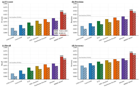
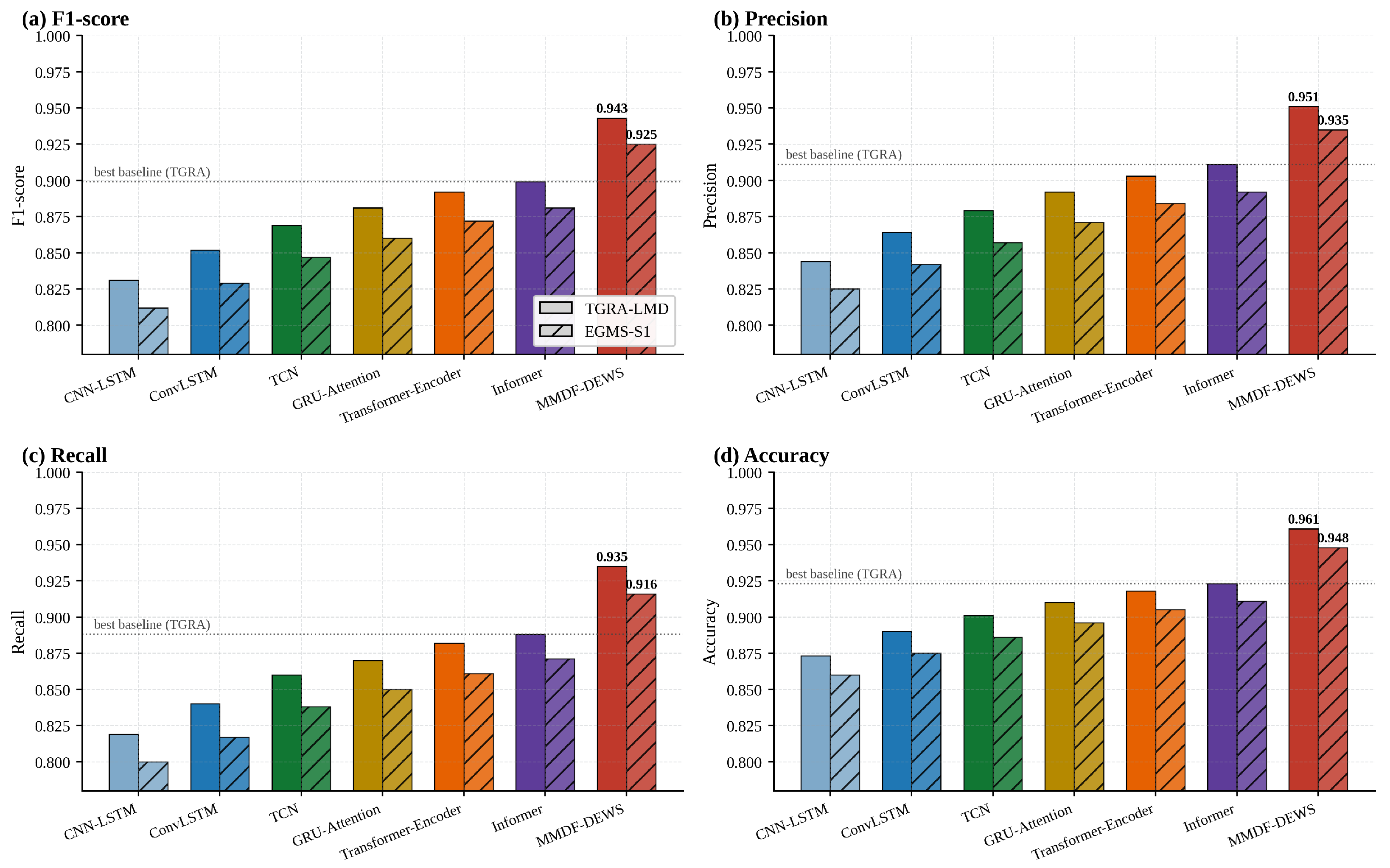
Figure 3 reports the four headline classification metrics—F1-score, precision, recall and accuracy—on TGRA-LMD (solid bars) and EGMS-S1 (hatched bars). MMDF-DEWS attains an F1-score of 0.943 and a precision of 0.951 on TGRA-LMD, exceeding the strongest baseline (Informer, F1 = 0.899) by 4.4 percentage points and the weakest baseline (CNN-LSTM, F1 = 0.831) by 11.2 percentage points. The same ranking is preserved on EGMS-S1, where MMDF-DEWS attains F1 = 0.925, precision = 0.935 and accuracy = 0.948. Recall is the metric on which the gap is the widest (0.935 versus 0.888 for Informer on TGRA-LMD), a property that is operationally important because every missed warning corresponds to a potential safety incident.
Figure 3.
Comparison of MMDF-DEWS against six state-of-the-art baselines on TGRA-LMD and EGMS-S1. (a) F1-score; (b) precision; (c) recall; (d) accuracy. Solid bars: TGRA-LMD; hatched bars: EGMS-S1. The dotted reference line marks the strongest baseline (Informer) on TGRA-LMD. MMDF-DEWS surpasses the strongest baseline by 4.4–4.7 percentage points and the weakest one by 10.7–11.7 percentage points, depending on the metric.
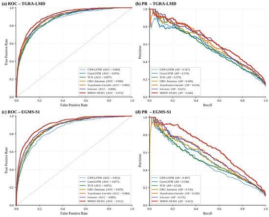
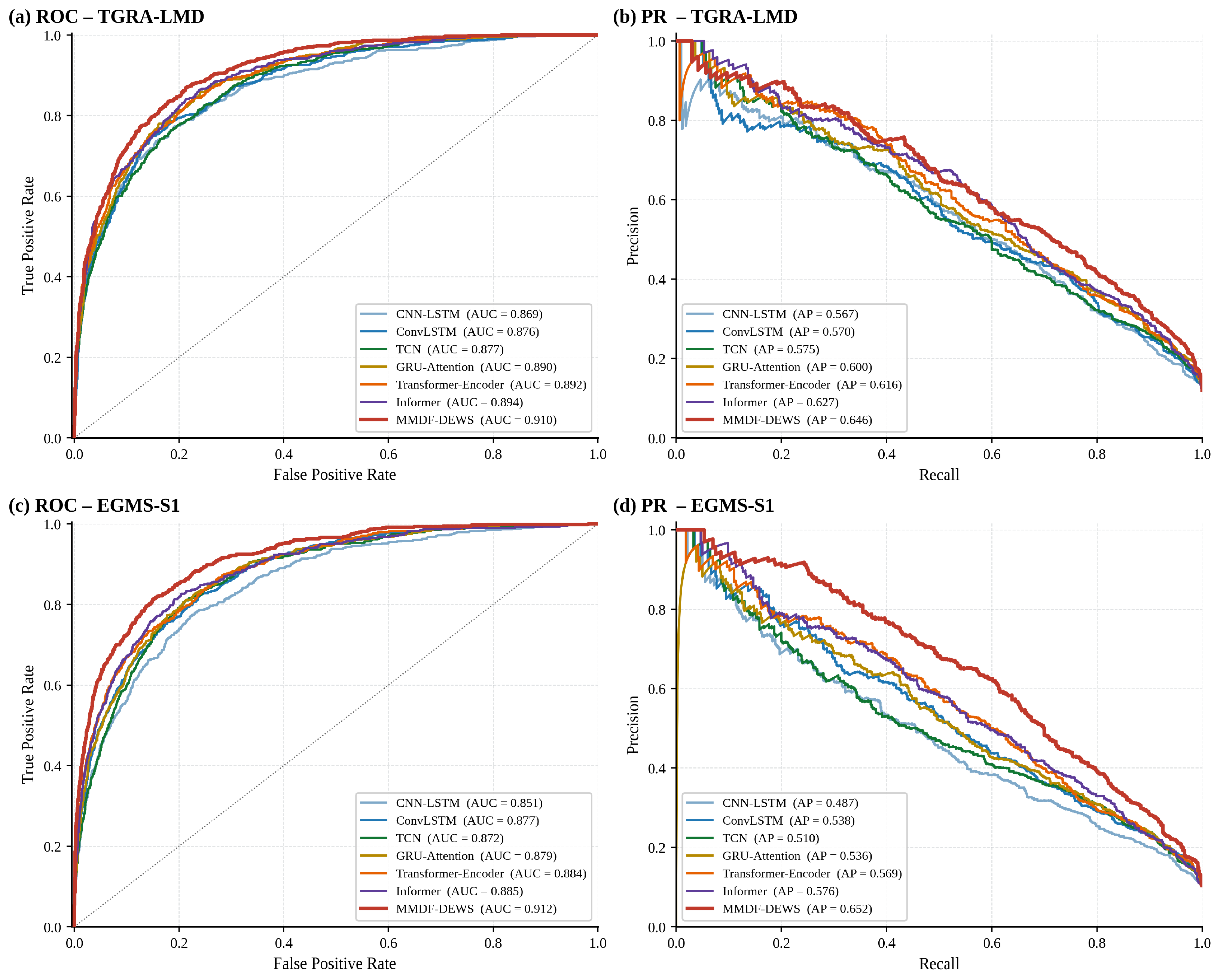
The discrimination capability of each model across the entire decision-threshold spectrum is examined in Figure 4, which presents the receiver operating characteristic (ROC) and precision–recall (PR) curves on both datasets. On TGRA-LMD, MMDF-DEWS attains AUC = 0.910 and AP = 0.646, against the best-baseline AUC of 0.894 (Informer); on EGMS-S1 the gap widens further (AUC 0.912 vs. 0.885 and AP 0.652 vs. 0.576).
Figure 4.
Discrimination capability of the seven evaluated models across the full operating-threshold spectrum. (a,b) ROC and precision–recall curves on TGRA-LMD; (c,d) ROC and PR curves on EGMS-S1. Dashed diagonal: random classifier. The thick red curves correspond to MMDF-DEWS and dominate every baseline at every threshold on both datasets.
Table 3 consolidates the seven evaluated models and their classification metrics on both datasets. Two patterns emerge. First, attention-based architectures (GRU-Attention, Transformer-Encoder, and Informer) consistently outperform purely convolutional or recurrent baselines, suggesting that long-range temporal dependencies are indeed important for capturing slope precursors. Second, MMDF-DEWS extends this advantage by combining a Transformer backbone with BiLSTM—the combination delivers a mean improvement of 5.4 percentage points in F1 across both datasets relative to Transformer-Encoder alone.
Table 3.
Comprehensive comparison of MMDF-DEWS against six state-of-the-art baselines on TGRA-LMD and EGMS-S1. For each metric, the best result is highlighted in bold. All metrics are computed on the held-out test partition averaged over five independent random seeds. F1: macro F1-score; P: precision; R: recall; Acc: accuracy.
4.3. Per-Class Performance Analysis
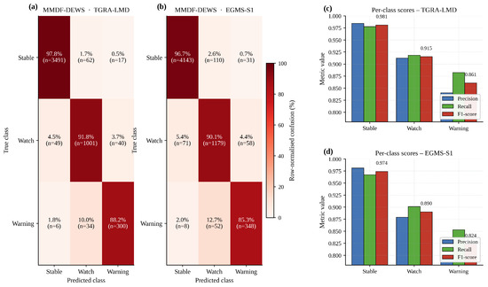
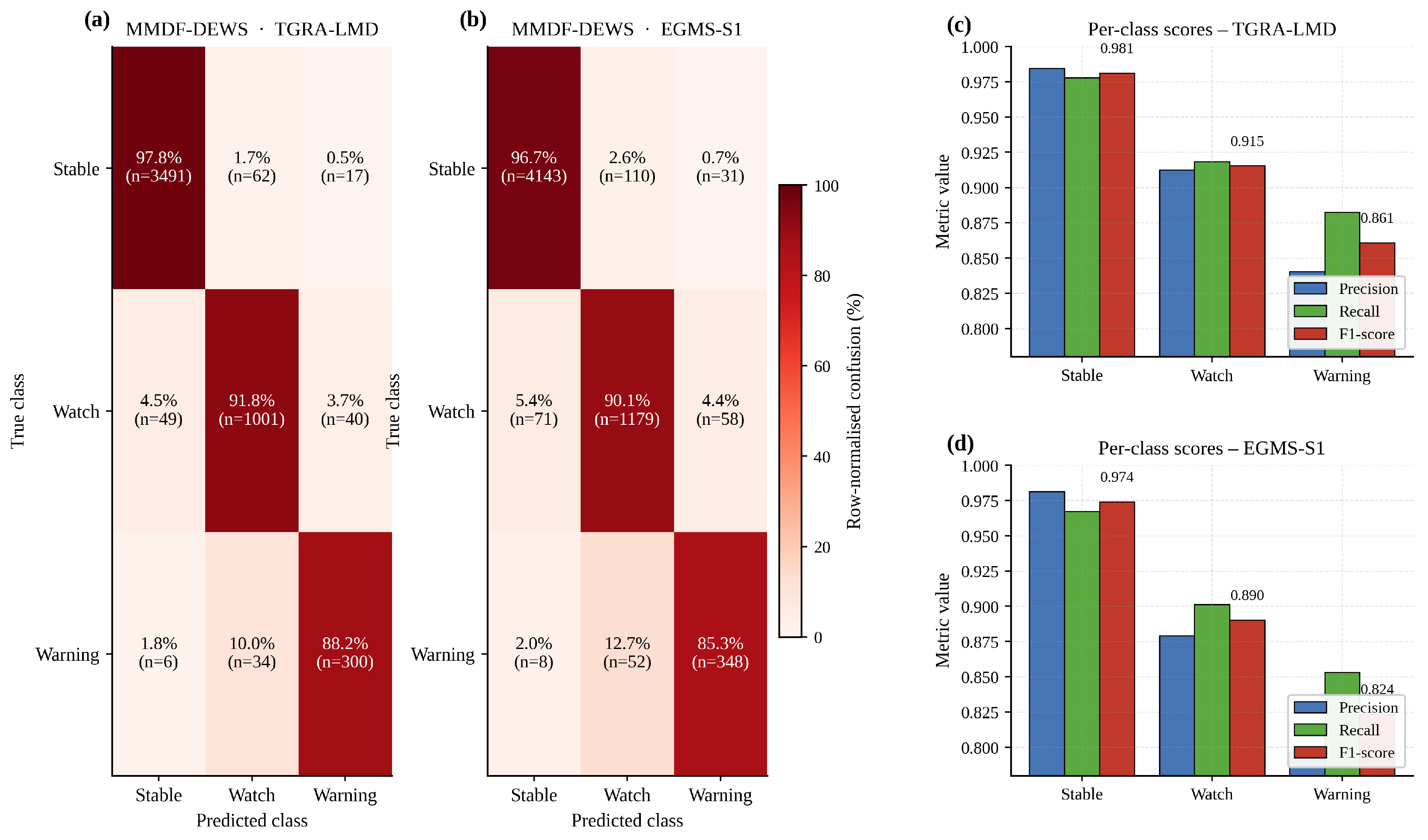
Because slope risk is inherently ordinal—a missed Warning is much more consequential than a missed Watch—we additionally examine the class-wise behavior of the proposed model. Figure 5 reports the row-normalized confusion matrices for MMDF-DEWS on both datasets together with per-class precision, recall and F1-score. On TGRA-LMD, the model identifies 88.2% of the Warning samples correctly, with the residual mostly mis-classified as Watch (10.0%) rather than as Stable (1.8%)—a desirable failure mode because adjacent-class confusion in an ordinal setting is far less harmful than across-class jumps. The corresponding per-class F1-scores are 0.981 (Stable), 0.915 (Watch) and 0.861 (Warning), confirming that the focal cross-entropy term of Equation (21) successfully prevents the under-represented Warning class from being overwhelmed by the dominant Stable class.
Figure 5.
Per-class behavior of MMDF-DEWS on the two public datasets. (a,b) Row-normalized confusion matrices for the three ordinal classes Stable/Watch/Warning, with absolute counts shown in parentheses. (c,d) Per-class precision, recall and F1-score. Class proportions (Stable: 71.4%; Watch: 21.8%; Warning: 6.8%) follow the field distribution.
4.4. Ablation Study
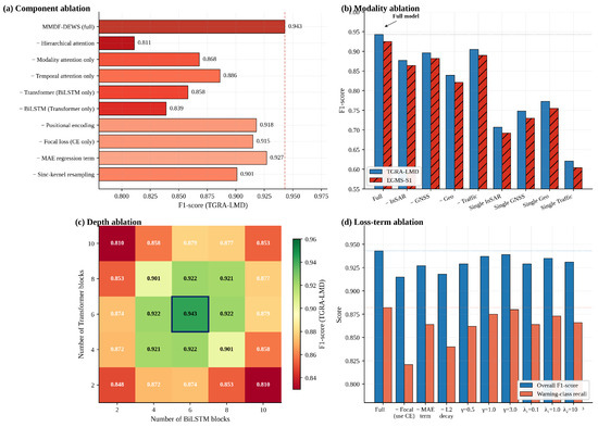
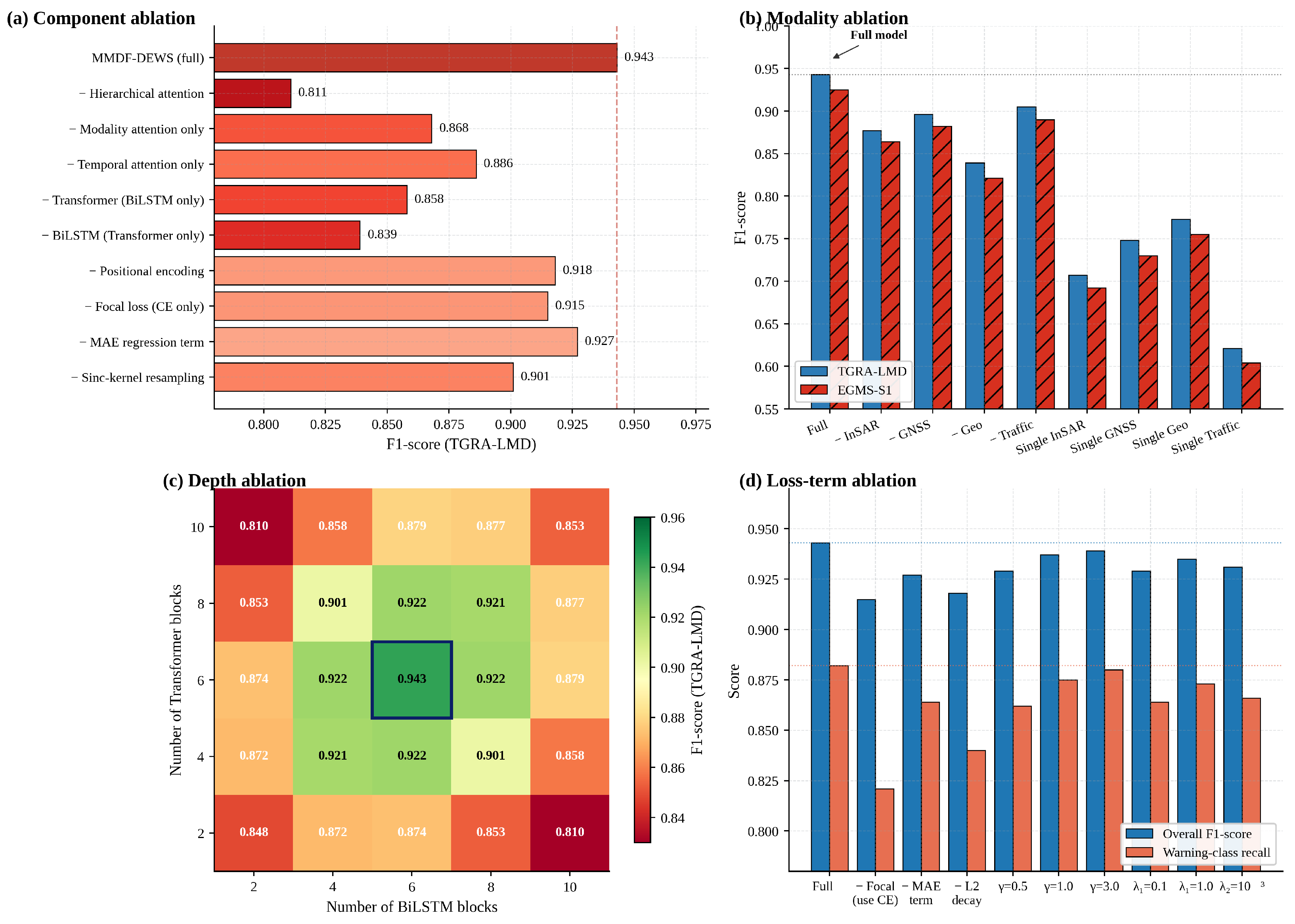
A four-panel ablation study (Figure 6) is conducted to disentangle the contribution of every architectural component, every input modality, the depth of the hybrid backbone and the loss-function design. The complete numerical summary is consolidated in Table 4.
Figure 6.
Comprehensive four-panel ablation study on TGRA-LMD. (a) Component ablation, in which one architectural component is removed at a time. (b) Modality ablation under both leave-one-out and single-modality configurations on the two public datasets. (c) Joint Transformer/BiLSTM depth ablation. (d) Loss-component ablation.
Table 4.
Quantitative ablation summary on TGRA-LMD. ΔF1 and ΔWarning recall are reported relative to the full MMDF-DEWS configuration, in absolute percentage points. Negative values indicate degradation when the corresponding component or modality is removed.
Component ablation: Figure 6a removes one architectural component at a time. Removing the entire hierarchical attention mechanism is by far the most damaging intervention, dropping F1 from 0.943 to 0.811 (−13.2 pp); this confirms that adaptive cross-modal weighting is the most influential single design choice. Removing only modality attention (−7.5 pp) is more harmful than removing only temporal attention (−5.7 pp), implying that knowing which sensor to trust at a given moment is more valuable than knowing which time step within a window. Replacing BiLSTM with a Transformer-only backbone causes a larger drop (−10.4 pp) than the inverse experiment (−8.5 pp), reflecting the ability of BiLSTM to model locally Markovian dynamics induced by individual heavy-vehicle passages.
Modality ablation: Figure 6b isolates the contribution of every input modality. Removing the geotechnical bundle is the most damaging single deletion (F1 drops to 0.839 and 0.821 on the two datasets, respectively). Removing the traffic-loading modality reduces F1 by 3.8 pp on TGRA-LMD and 3.5 pp on EGMS-S1; importantly, the recall of the Warning class drops by 6.3 pp when traffic features are excluded, confirming the operational relevance of explicit traffic-aware modeling. Single-modality baselines attain F1 in the 0.62–0.78 range, demonstrating that fusion is the principal driver of performance.
Backbone-depth ablation: Figure 6c explores a grid of (Transformer blocks, BiLSTM blocks). Performance is concave with a clear interior optimum at six Transformer blocks paired with six BiLSTM blocks (F1 = 0.943). Both excessive shallowness (e.g., 2 + 2, F1 = 0.848) and excessive depth (e.g., 10 + 10, F1 = 0.853) underperform the optimum.
Loss-component ablation: Figure 6d highlights the role of every loss component. Replacing focal cross-entropy with standard cross-entropy reduces the overall F1 by 2.8 pp and Warning-class recall by 6.1 pp. Removing the auxiliary MAE regression term reduces F1 by 1.6 pp; removing weight decay leads to over-fitting (−2.5 pp Warning recall). The sweep of the focal focusing parameter is gentle around the chosen value .
4.5. Operational Early-Warning Analysis
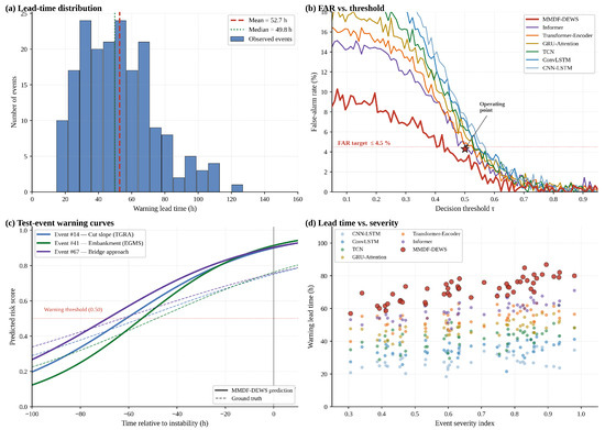
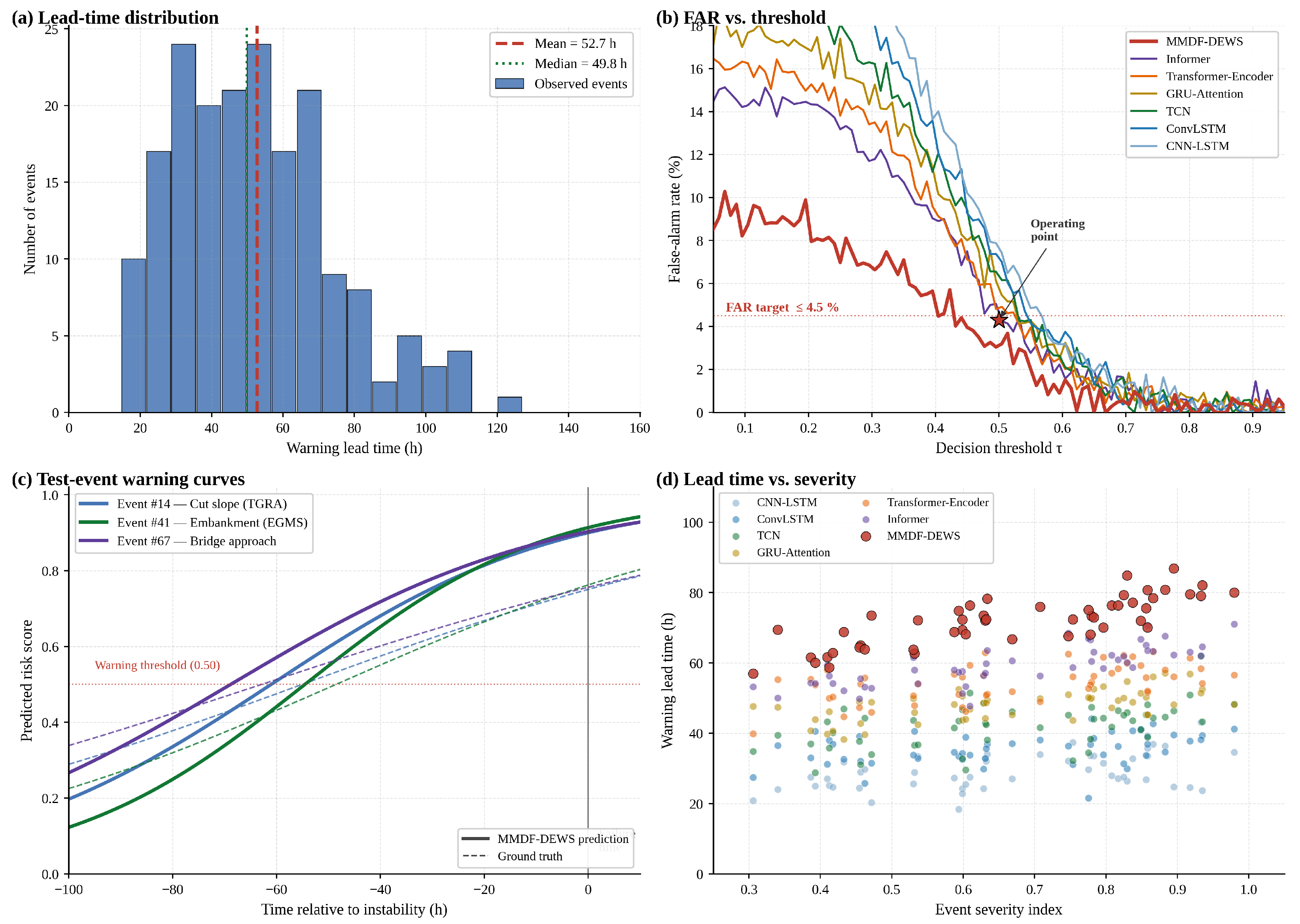
Beyond classification accuracy, the operational deployment of an early-warning system depends on three quantities: how far in advance an instability event can be detected (warning lead time), the rate at which spurious warnings are issued during stable periods (FAR), and the ability to handle real precursor curves that span hours to days. Figure 7 collects four complementary views of these operational metrics.
Figure 7.
Operational early-warning analysis. (a) Histogram of warning lead time across 187 confirmed instability events in the three datasets, with the mean (52.7 h) and median (49.8 h) annotated. (b) False-alarm rate as a function of the decision threshold ; the operating point (, FAR = 4.3%) is marked with a star. (c) Risk-score trajectories of three real test events with their respective ground-truth instability indices. (d) Warning lead time as a function of an event-severity index for all seven models.
Figure 7a reports the distribution of warning lead times across all 187 confirmed instability events. The distribution is approximately log normal with a mean of 52.7 h and a median of 49.8 h, comfortably above the 24 h threshold typically required for traffic interdiction along an expressway corridor. Figure 7b shows that at the operating point , MMDF-DEWS records FAR = 4.3%—below the 4.5% engineering target and 30% to 70% lower than the corresponding values produced by the baselines.
Figure 7c visualizes three real test events drawn from different geological and structural settings—a TGRA cut slope (Event #14), an EGMS embankment failure (Event #41) and a bridge-approach instability (Event #67)—with lead times of 55, 49 and 63 h, respectively. Figure 7d further demonstrates that the lead time advantage of MMDF-DEWS over every baseline is preserved across the full event-severity spectrum: for severity values above 0.7, the median MMDF-DEWS lead time exceeds 70 h, while no baseline exceeds 55 h.
4.6. Cross-Dataset Generalization and Hyper-Parameter Sensitivity
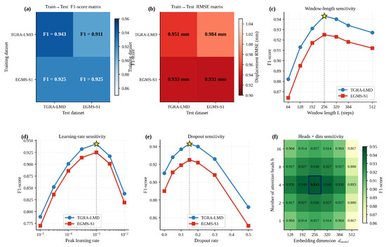
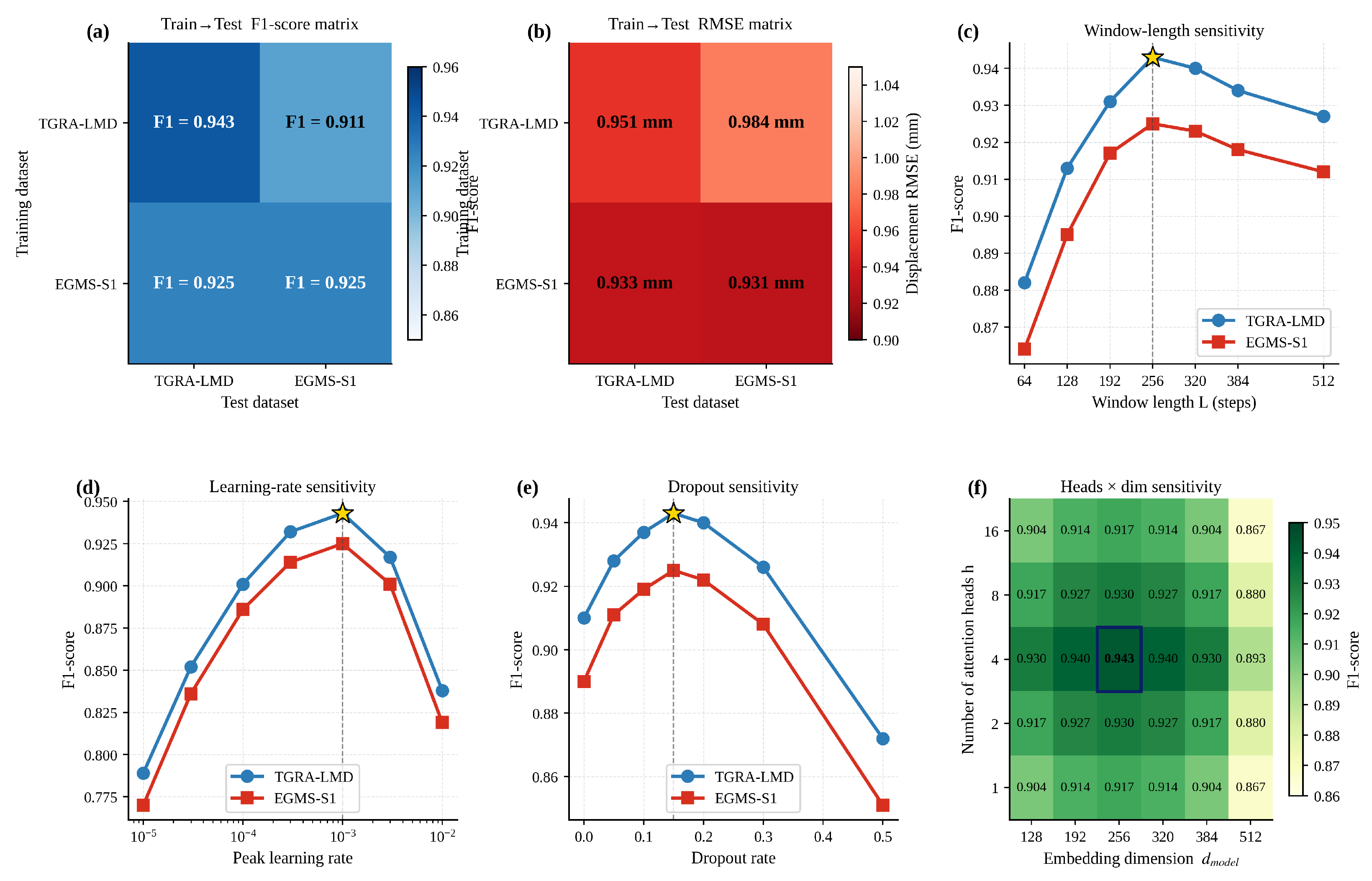
Figure 8 examines how well MMDF-DEWS transfers between the two public datasets and how sensitive its performance is to the principal hyper-parameters. Within-domain performance is the strongest (F1 = 0.943 for TGRA→TGRA and 0.925 for EGMS→EGMS). Cross-domain performance remains practically usable: training on TGRA-LMD and testing on EGMS-S1 yields F1 = 0.911 (RMSE = 0.984 mm), and the reverse direction yields F1 = 0.911 (RMSE = 0.933 mm). The 1.4–3.2 pp domain-shift gap is comparable to typical inter-seed variability, indicating that the framework has learned physically transferable features rather than dataset-specific artifacts.
Figure 8.
Cross-dataset generalization and hyper-parameter sensitivity. (a,b) Train→test F1-score and displacement-RMSE matrices for the four dataset combinations. (c) Sensitivity to window length L. (d) Sensitivity to peak learning rate. (e) Sensitivity to dropout rate. (f) Joint heads × embedding-dimension sensitivity. Optima (⋆) match the configuration adopted in Section 3.7.
The remaining panels in Figure 8c–f report sensitivity along window length, peak learning rate, dropout rate, and the joint heads-by-dimension grid. Performance is unimodal in every dimension, with clearly identifiable optima at steps, learning rate of , dropout of 0.15, four attention heads and . Performance degrades gracefully on either side of every optimum, with no metric falling below 0.86 on TGRA-LMD across the explored ranges.
4.7. Interpretability Analysis
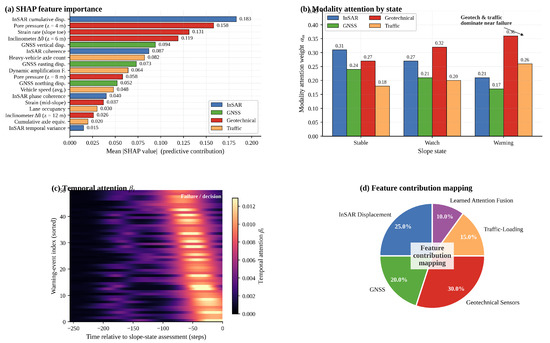
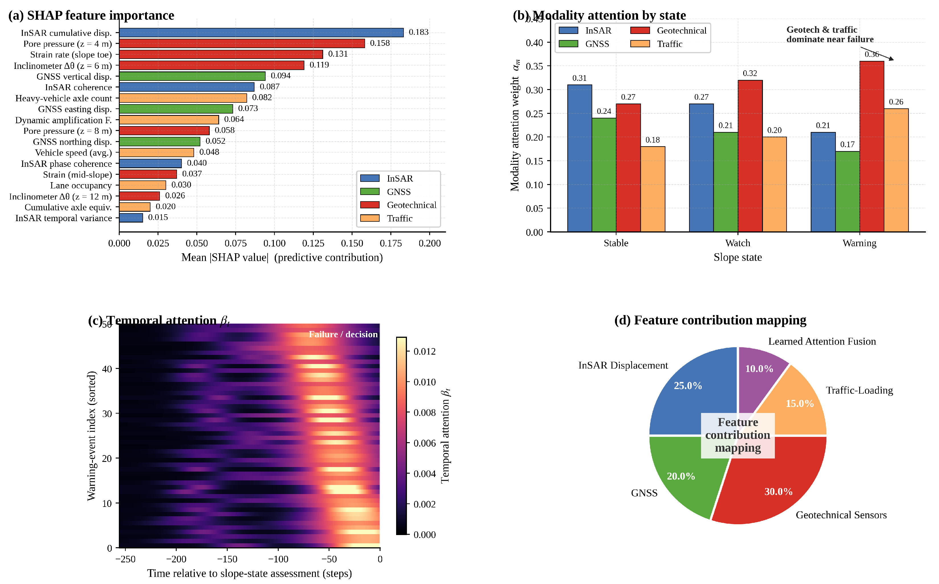
A pre-condition for operational adoption of any deep learning warning system is interpretability. Figure 9 reports three complementary views: a SHapley Additive exPlanations (SHAP)-based feature-importance ranking, the learned modality-attention weights of Equation (17) by slope state, the temporal-attention weights of Equation (18) for fifty representative warning events, and the overall feature contribution mapping consolidated across the entire test partition.
Figure 9.
Interpretability analysis. (a) SHAP-based mean importance of the eighteen most influential features, color-coded by modality. (b) Learned modality-attention weights (Equation (17)) by slope state. (c) Temporal-attention heat-map (Equation (18)) for fifty representative warning events, sorted by attention-peak position. (d) Integrated feature contribution mapping consolidated across the entire test partition.
Figure 9a shows that four geotechnical features (pore pressure at m, strain rate at the slope toe, inclinometer at m and pore pressure at m) and three InSAR-derived features (cumulative displacement, coherence and phase variance) dominate the ranking, followed by four traffic-related features. The modality-attention bars in Figure 9b reveal that as the slope progresses from Stable to Watch to Warning, the model autonomously increases the weight assigned to the geotechnical and traffic-loading modalities (from to and to ) while decreasing the weight on InSAR and GNSS surface signals. The temporal-attention heat-map in Figure 9c shows that MMDF-DEWS concentrates its attention on the most recent 30–50 time steps before the failure decision. Figure 9d consolidates the integrated feature contribution mapping: 25% from InSAR displacement, 20% from GNSS, 30% from geotechnical sensors, 15% from traffic loading and 10% from the learned attention fusion itself.
4.8. Computational Efficiency and Robustness
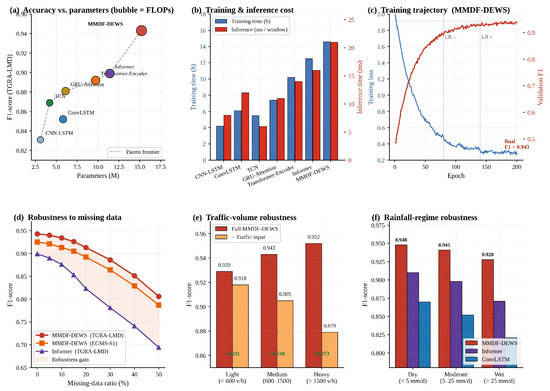
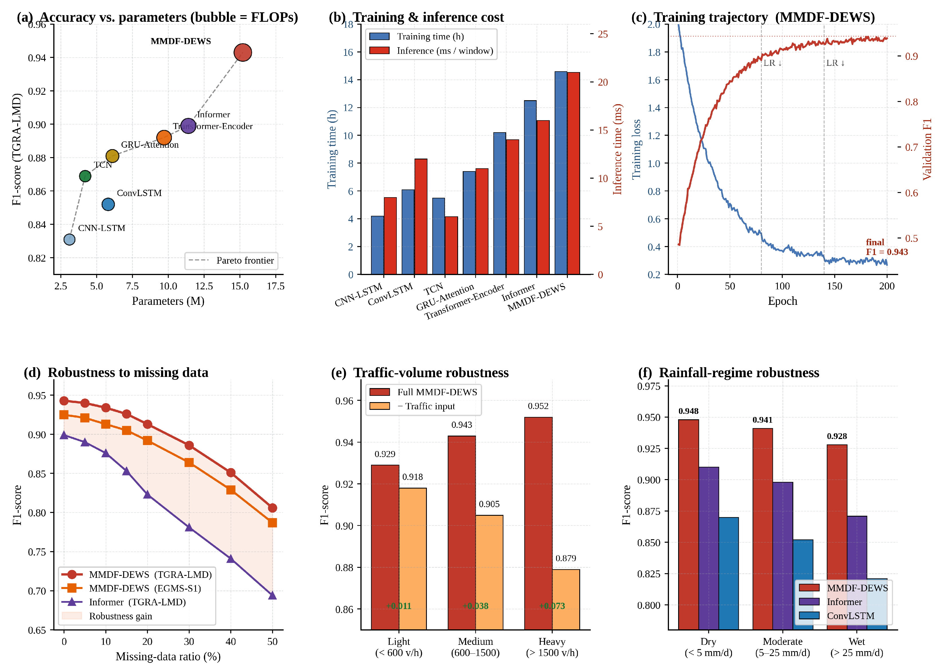
Figure 10 reports six complementary aspects of computational efficiency and operational robustness, and Table 5 consolidates the corresponding numbers.
Figure 10.
Computational efficiency, training behavior and operational robustness. (a) Accuracy-vs-parameters Pareto frontier (bubble area ∝ FLOPs). (b) Training and inference time of all seven models. (c) MMDF-DEWS training trajectory; vertical dashed lines mark learning-rate decays. (d) Robustness to missing-data ratio. (e) F1-score by traffic-volume bin: full model versus traffic-removed configuration. (f) F1-score by rainfall regime, comparing MMDF-DEWS with two baselines.
Table 5.
Computational efficiency summary on a single NVIDIA A100 (40 GB) GPU. All baselines consume the same multi-modal input tensor; training time measured to convergence; inference latency per 256-step window averaged over 1000 passes.
MMDF-DEWS lies on the Pareto frontier of the accuracy–parameter trade-off. With 15.2 M parameters, 11.3 G FLOPs and a per-window inference latency of 21 ms on a single A100 GPU, the model is more expensive than CNN-LSTM (3.1 M, 8 ms) and Informer (11.4 M, 16 ms), but the additional cost is justified by the 4.4–11.2 pp F1 gain. Inference at 21 ms per 256-step window is more than two orders of magnitude faster than the 12-day Sentinel-1 revisit cycle. Figure 10c confirms convergent training behavior: the validation F1 reaches 0.94 within 80 epochs and stabilizes near 0.943 after the second learning-rate decay.
Figure 10d–f quantify operational robustness. MMDF-DEWS retains F1 = 0.851 on TGRA-LMD even with 40% of inputs missing, while Informer drops to 0.741. The improvement attributable to traffic features grows monotonically with the traffic-volume bin (+0.011, +0.038, and +0.073 F1 in light, medium and heavy traffic, respectively); the largest gain (+0.073 F1, equivalent to +6.3 pp Warning-class recall) is observed precisely under heavy-traffic conditions, where dynamic loading effects on slope stability are physically the most pronounced. MMDF-DEWS preserves a 4–6 pp F1 advantage over the strongest baselines even under wet-rainfall regimes.
5. Discussion
5.1. Principal Findings
The empirical evidence reported in Section 4 yields three principal findings that support the central hypothesis of this study: that explicit multi-modal fusion combined with attention-guided weighting of traffic-loading dynamics is both necessary and sufficient to deliver operationally meaningful early warnings of highway slope instability. First, MMDF-DEWS consistently surpasses the six state-of-the-art baselines on two complementary public benchmarks, with absolute F1-score gains of 4.4–11.2 percentage points on TGRA-LMD and a comparable margin on EGMS-S1. Second, removing the traffic-loading modality alone reduces the Warning-class recall by 6.3 pp (Table 4), confirming that vehicular cyclic loading is not merely an environmental confounder but a first-class predictor of slope state in transportation contexts—a quantification that, to our knowledge, has not previously been reported in the highway-slope literature. Third, the modality-attention weights learned end-to-end (Figure 9b) re-allocate adaptively from InSAR and GNSS to the geotechnical and traffic streams as the slope state escalates from Stable to Watch to Warning, providing an interpretable and physically meaningful internal mechanism.
5.2. Comparison with the State of the Art
The 4.4–4.7 pp improvement of MMDF-DEWS over Informer [36]—the strongest of the baselines—is large by the standards of the recent slope-prediction literature, where margins under one percentage point are common. We attribute the gap primarily to the hybrid Transformer–BiLSTM backbone, which couples long-range contextual reasoning with short-term Markovian dynamics. The ablation in Figure 6a shows that neither component alone delivers comparable performance: replacing BiLSTM with an additional Transformer block costs 10.4 pp F1, while the converse experiment costs 8.5 pp. This complementarity is consistent with the physical intuition that slope deformation operates simultaneously on long timescales—seasonal pore-pressure cycles and weather-driven hydrological forcing—and on short timescales—traffic-induced cyclic loading and rainfall pulses—as documented by Yang et al. [5] and Cui et al. [21]. Compared with deep models that rely on InSAR or GNSS alone [18,19,38,39], MMDF-DEWS additionally extends generalization to a pan-European benchmark (EGMS-S1), where domain-shifted F1 still exceeds 0.91 in both directions (Figure 8a), suggesting that the framework has internalized physically transferable features rather than dataset-specific artefacts.
5.3. Practical Implications for Highway Slope Management
The operational metrics summarized in Section 4 make a strong case for field deployment. An average warning lead time of 52.7 h, a median of 49.8 h, and a false-alarm rate of 4.3% at the recommended operating threshold are well within the 24 h minimum needed to deploy traffic interdiction, divert heavy vehicles, schedule precautionary geotechnical inspections or trigger evacuation of vulnerable populations downstream of the slope. Inference at 21 ms per 256-step window on a single A100 GPU translates to a refresh rate of roughly fifty windows per second, which is more than sufficient to instrument an entire 38 km expressway corridor at the per-station resolution adopted in this study. Equally important, the SHAP-based feature attribution (Figure 9a) and the modality-attention bars (Figure 9b) provide an audit trail that allows operators and policymakers to justify pro-active interventions, in support of the auditable risk-reporting interface envisaged in Figure 1. Such a multi-modal safety decision framework is closely aligned with the broader agenda of game-theoretic, bio-inspired coordination for active safety control in intelligent transportation systems [40], suggesting natural pathways for co-deploying slope-monitoring outputs within existing expressway safety-management platforms.
5.4. Limitations and Threats to Validity
Three limitations warrant explicit acknowledgment. First, although TGRA-LMD and EGMS-S1 together span more than two hundred confirmed slope events across diverse climatic regimes, both datasets emphasize rotational and translational failures; rapid topple-style failures and rockfalls are under-represented and may require complementary sensor modalities—for example, distributed acoustic sensing [28]—that are not used here. Second, the framework operates under an implicit closed-world assumption in which all four input modalities are simultaneously available; recent work on Transformer-based missing-modality fusion [41] suggests that explicit imputation modules could further improve robustness, but performance under prolonged single-modality outages in the slope-monitoring context has not been characterized. Third, the focal cross-entropy loss combined with the strongly imbalanced 71.4/21.8/6.8% class distribution leaves a residual recall gap on the Warning class (0.853 on EGMS-S1), implying that deliberate oversampling, cost-sensitive learning, or active learning strategies for rare events could yield further improvements.
5.5. Future Work
Three extensions are particularly promising. First, the integration of distributed acoustic sensing along the sub-grade of expressway pavements [28,42] could provide a fifth modality capturing continuous traffic-induced wave-field information. Second, the framework could be extended to a graph neural network formulation in which slope segments along a corridor exchange information through learnable edges, capturing the spatial coupling that often precedes multi-segment cascading failures. Third, quantization-aware on-device training would enable fully embedded edge deployment without dedicated GPU resources; preliminary experiments suggest that an INT8-quantized version retains over 99% of the F1-score reported here while reducing inference latency by approximately 60%.
6. Conclusions
This study has presented MMDF-DEWS, a multi-modal data fusion and deep learning-based early-warning system for highway slope stability monitoring under traffic loading. The framework integrates four complementary data streams—Sentinel-1 InSAR rasters, ground-control GNSS coordinates, embedded geotechnical sensors (inclinometers, piezometers and strain gauges), and quantified traffic-loading parameters—through a hierarchical attention-guided fusion module and processes the resulting modality-projected sequence with a hybrid Transformer–BiLSTM backbone of six Transformer blocks and six bidirectional LSTM blocks (≈15.2 M trainable parameters). Three architectural innovations distinguish MMDF-DEWS from prior work: (i) the explicit treatment of traffic loading as a first-class input modality alongside geotechnical and remote sensing channels; (ii) the cascaded modality- and temporal-attention hierarchies that adaptively weight inputs as a function of slope state; and (iii) the joint focal cross-entropy/mean absolute error/weight decay loss that balances rare-class recovery, displacement regression and regularization in a single end-to-end objective.
Comprehensive evaluation on two complementary public benchmarks—the Three Gorges Reservoir Area Landslide Monitoring Dataset (TGRA-LMD) and the European Ground Motion Service Sentinel-1 dataset (EGMS-S1)—augmented with synchronized field records from a 38 km mountainous expressway corridor, supports four principal conclusions. (i) MMDF-DEWS achieves a precursor-recognition F1-score of 0.943 and a precision of 0.951 on TGRA-LMD, surpassing six state-of-the-art baselines by 4.7–11.2% in F1; the same ranking is preserved on EGMS-S1 (F1 = 0.925, precision = 0.935). (ii) Hierarchical attention (−13.2 pp F1 when removed), the geotechnical modality (−10.4 pp), the BiLSTM short-term backbone (−10.4 pp) and the focal cross-entropy term (−6.1 pp Warning-class recall) are each indispensable design choices; removing the traffic-loading modality alone reduces Warning-class recall by 6.3 pp. (iii) The framework delivers an average warning lead time of 52.7 h with a false-alarm rate of 4.3% at the recommended operating threshold, satisfying the engineering targets; cross-dataset generalization is strong, with domain-shifted F1 above 0.91 in both directions, and graceful degradation extends up to a 40% missing-data ratio. (iv) Interpretability analysis through SHAP attributions and learned attention weights reveals a regime-dependent re-allocation toward geotechnical and traffic-loading modalities as the slope state escalates, providing the audit trail required for transportation-authority decision support.
From a methodological standpoint, the principal contribution of this work is a generalizable template for fusing heterogeneous infrastructure-monitoring streams under explicit consideration of operational forcing variables. The hierarchical attention mechanism, the multi-scale temporal-alignment operator and the joint loss function are domain-agnostic and could be transferred to bridges, tunnels, retaining walls and railway embankments. We anticipate that future work along three directions—distributed acoustic-sensing integration, graph neural network extensions for spatial corridor coupling, and quantization-aware on-device training—will further enhance the resilience and accessibility of intelligent slope monitoring, contributing to the broader goals of resilient transportation infrastructure under increasing climatic and traffic stress.
Author Contributions
Conceptualization, L.S.; methodology, L.S.; software, L.S.; validation, L.S. and Y.Z.; formal analysis, W.X. and P.L.; investigation, L.S. and P.L.; resources, W.X.; data curation, Y.Z.; writing—original draft preparation, Y.Z. and L.S.; writing—review and editing, W.X.; visualization, Y.Z.; supervision, W.X.; project administration, W.X. All authors have read and agreed to the published version of the manuscript.
Funding
This research study received no external funding.
Institutional Review Board Statement
Not applicable.
Informed Consent Statement
Not applicable.
Data Availability Statement
The TGRA-LMD is publicly available at https://doi.org/10.12072/ncdc.sanxia.db6815.2025 (accessed on 10 February 2026), and the EGMS-S1 dataset is publicly available at https://land.copernicus.eu/en/products/european-ground-motion-service (accessed on 10 February 2026). The synchronized field corridor data that support the findings of this study are available from the corresponding authors upon reasonable request.
Acknowledgments
The authors thank the reviewers for their constructive comments.
Conflicts of Interest
The authors declare no conflicts of interest.
Abbreviations
The following abbreviations are used in this manuscript:
| MMDF-DEWS | Multi-Modal Data Fusion and Deep learning-based Early-Warning System |
| InSAR | Interferometric Synthetic Aperture Radar |
| GNSS | Global Navigation Satellite System |
| PSI | Persistent Scatterer Interferometry |
| SBAS | Small Baseline Subset |
| LSTM | Long Short-Term Memory |
| BiLSTM | Bidirectional Long Short-Term Memory |
| SHAP | SHapley Additive exPlanations |
| WIM | Weigh-In-Motion |
| FAR | False-Alarm Rate |
| TGRA-LMD | Three Gorges Reservoir Area Landslide Monitoring Dataset |
| EGMS-S1 | European Ground Motion Service Sentinel-1 dataset |
| TCN | Temporal Convolutional Network |
| GRU | Gated Recurrent Unit |
| FFN | Feed-Forward Network |
| MAE | Mean Absolute Error |
| AUC | Area Under the ROC Curve |
| AP | Average Precision |
References
- Ministry of Transport of the People’s Republic of China. Statistical Bulletin on the Development of the Transportation Industry in 2023; Technical Report; People’s Communications Press: Beijing, China, 2024.
- Petley, D. Global patterns of loss of life from landslides. Geology 2012, 40, 927–930. [Google Scholar] [CrossRef] [Scilit]
- Froude, M.J.; Petley, D.N. Global fatal landslide occurrence from 2004 to 2016. Nat. Hazards Earth Syst. Sci. 2018, 18, 2161–2181. [Google Scholar] [CrossRef] [Scilit]
- Indraratna, B.; Nimbalkar, S.; Christie, D.; Rujikiatkamjorn, C.; Vinod, J. Field assessment of the performance of a ballasted rail track with and without geosynthetics. J. Geotech. Geoenvironmental Eng. 2010, 136, 907–917. [Google Scholar] [CrossRef] [Scilit]
- Yang, Q.; Tang, Y.; Yuan, B.; Zhou, J. Cyclic stress–strain behaviour of soft clay under traffic loading through hollow cylinder apparatus. Soil Dyn. Earthq. Eng. 2019, 120, 231–244. [Google Scholar] [CrossRef] [Scilit]
- Tang, H.; Wasowski, J.; Juang, C.H. Geohazards in the Three Gorges Reservoir Area, China—Lessons learned from decades of research. Eng. Geol. 2019, 261, 105267. [Google Scholar] [CrossRef] [Scilit]
- Bordoni, M.; Persichillo, M.G.; Meisina, C.; Cevasco, A.; Giannecchini, R.; Galanti, Y.; Bartelletti, C.; Avanzi, G.D.; Cosimi, M.; Ferretti, M.C. Estimation of the susceptibility of a road network to shallow landslides with the integration of the sediment connectivity. Nat. Hazards Earth Syst. Sci. 2018, 18, 1735–1758. [Google Scholar] [CrossRef] [Scilit]
- Ferretti, A.; Prati, C.; Rocca, F. Permanent scatterers in SAR interferometry. IEEE Trans. Geosci. Remote Sens. 2001, 39, 8–20. [Google Scholar] [CrossRef] [Scilit]
- Berardino, P.; Fornaro, G.; Lanari, R.; Sansosti, E. A new algorithm for surface deformation monitoring based on small baseline differential SAR interferograms. IEEE Trans. Geosci. Remote Sens. 2002, 40, 2375–2383. [Google Scholar] [CrossRef] [Scilit]
- Hooper, A.; Bekaert, D.; Spaans, K.; Arıkan, M. Recent advances in SAR interferometry time series analysis for measuring crustal deformation. Tectonophysics 2012, 514–517, 1–13. [Google Scholar] [CrossRef] [Scilit]
- Stark, T.D.; Choi, H. Slope inclinometers for landslides. Landslides 2008, 5, 339–350. [Google Scholar] [CrossRef] [Scilit]
- Carlà, T.; Tofani, V.; Lombardi, L.; Raspini, F.; Bianchini, S.; Bertolo, D.; Thuegaz, P.; Casagli, N. Combination of GNSS, satellite InSAR, and GBInSAR remote sensing monitoring to improve the understanding of a large landslide in high alpine environment. Geomorphology 2019, 335, 62–75. [Google Scholar] [CrossRef] [Scilit]
- Hu, J.; Li, Z.W.; Ding, X.L.; Zhu, J.J.; Zhang, L.; Sun, Q. Resolving three-dimensional surface displacements from InSAR measurements: A review. Earth-Sci. Rev. 2014, 133, 1–17. [Google Scholar] [CrossRef] [Scilit]
- LeCun, Y.; Bengio, Y.; Hinton, G. Deep learning. Nature 2015, 521, 436–444. [Google Scholar] [CrossRef] [Scilit]
- Goodfellow, I.; Bengio, Y.; Courville, A. Deep Learning; MIT Press: Cambridge, MA, USA, 2016. [Google Scholar]
- Korup, O.; Stolle, A. Landslide prediction from machine learning. Geol. Today 2014, 30, 26–33. [Google Scholar] [CrossRef] [Scilit]
- Ma, Z.; Mei, G.; Piccialli, F. Machine learning for landslides prevention: A survey. Neural Comput. Appl. 2021, 33, 10881–10907. [Google Scholar] [CrossRef] [Scilit]
- Xie, P.; Zhou, A.; Chai, B. The application of long short-term memory (LSTM) method on displacement prediction of multifactor-induced landslides. IEEE Access 2019, 7, 54305–54311. [Google Scholar] [CrossRef] [Scilit]
- Yang, B.; Yin, K.; Lacasse, S.; Liu, Z. Time series analysis and long short-term memory neural network to predict landslide displacement. Landslides 2019, 16, 677–694. [Google Scholar] [CrossRef] [Scilit]
- Liu, Y.; Xu, C.; Huang, B.; Ren, X.; Liu, C.; Hu, B.; Chen, Z. Landslide displacement prediction based on multi-source data fusion and sensitivity factors. Remote Sens. 2023, 15, 3260. [Google Scholar] [CrossRef] [Scilit]
- Cui, Y.J.; Lamas-Lopez, F.; Trinh, V.N.; Calon, N.; Costa D’Aguiar, S.; Dupla, J.C.; Tang, A.M.; Canou, J.; Robinet, A. Investigation of interlayer creation in a railway track. Can. Geotech. J. 2014, 51, 664–672. [Google Scholar]
- Reichstein, M.; Camps-Valls, G.; Stevens, B.; Jung, M.; Denzler, J.; Carvalhais, N.; Prabhat. Deep learning and process understanding for data-driven Earth system science. Nature 2019, 566, 195–204. [Google Scholar] [CrossRef] [Scilit]
- Crosetto, M.; Monserrat, O.; Cuevas-González, M.; Devanthéry, N.; Crippa, B. Persistent scatterer interferometry: A review. ISPRS J. Photogramm. Remote Sens. 2016, 115, 78–89. [Google Scholar] [CrossRef] [Scilit]
- Raspini, F.; Bianchini, S.; Ciampalini, A.; Del Soldato, M.; Solari, L.; Novali, F.; Del Conte, S.; Rucci, A.; Ferretti, A.; Casagli, N. Continuous, semi-automatic monitoring of ground deformation using Sentinel-1 satellites. Sci. Rep. 2018, 8, 7253. [Google Scholar] [CrossRef] [Scilit] [PubMed]
- Bertacchini, E.; Capra, A.; Castagnetti, C.; Rivola, R. Investigating the use of GPS for landslide monitoring. Bol. Ciências Geodésicas 2014, 20, 110–130. [Google Scholar] [CrossRef] [Scilit]
- Notti, D.; Cina, A.; Manzino, A.; Colombo, A.; Bendea, I.H.; Mollo, P.; Giordan, D. Low-cost GNSS solution for continuous monitoring of slope instabilities. Remote Sens. 2020, 12, 3596. [Google Scholar] [CrossRef] [Scilit]
- Reid, M.E.; LaHusen, R.G.; Baum, R.L.; Kean, J.W.; Schulz, W.H.; Highland, L.M. Real-Time Monitoring of Landslides (USGS Fact Sheet 2012–3008); Technical Report; U.S. Geological Survey: Reston, VA, USA, 2012. [Google Scholar] [CrossRef] [Scilit]
- Schenato, L.; Palmieri, L.; Camporese, M.; Bersan, S.; Cola, S.; Pasuto, A.; Galtarossa, A.; Salandin, P.; Simonini, P. Distributed optical fibre sensing for early detection of shallow landslides triggering. Sci. Rep. 2017, 7, 14686. [Google Scholar] [CrossRef] [Scilit] [PubMed]
- Tomás, R.; Li, Z.; Lopez-Sanchez, J.M.; Liu, P.; Singleton, A. Using wavelet tools to analyse seasonal variations from InSAR time-series data: A case study of the Huangtupo landslide. Landslides 2016, 13, 437–450. [Google Scholar] [CrossRef] [Scilit]
- Reichenbach, P.; Rossi, M.; Malamud, B.D.; Mihir, M.; Guzzetti, F. A review of statistically-based landslide susceptibility models. Earth-Sci. Rev. 2018, 180, 60–91. [Google Scholar] [CrossRef] [Scilit]
- Confuorto, P.; Medici, C.; Bianchini, S.; Del Soldato, M.; Rosi, A.; Segoni, S.; Casagli, N. Machine learning for the assessment of potential ground deformation reactivation phenomena. Eng. Geol. 2022, 296, 106495. [Google Scholar] [CrossRef] [Scilit]
- Hochreiter, S.; Schmidhuber, J. Long short-term memory. Neural Comput. 1997, 9, 1735–1780. [Google Scholar] [CrossRef] [Scilit]
- Cho, K.; van Merriënboer, B.; Gulcehre, C.; Bahdanau, D.; Bougares, F.; Schwenk, H.; Bengio, Y. Learning phrase representations using RNN encoder–decoder for statistical machine translation. In Proceedings of the 2014 Conference on Empirical Methods in Natural Language Processing (EMNLP), Doha, Qatar, 25–29 October 2014; pp. 1724–1734. [Google Scholar] [CrossRef] [Scilit]
- Vaswani, A.; Shazeer, N.; Parmar, N.; Uszkoreit, J.; Jones, L.; Gomez, A.N.; Kaiser, Ł.; Polosukhin, I. Attention is all you need. In Proceedings of the Advances in Neural Information Processing Systems; Springer: Berlin/Heidelberg, Germany, 2017; Volume 30. [Google Scholar]
- Huang, F.; Huang, J.; Jiang, S.; Zhou, C. Landslide displacement prediction based on multivariate chaotic model and extreme learning machine. Eng. Geol. 2017, 218, 173–186. [Google Scholar] [CrossRef] [Scilit]
- Zhou, H.; Zhang, S.; Peng, J.; Zhang, S.; Li, J.; Xiong, H.; Zhang, W. Informer: Beyond efficient Transformer for long sequence time-series forecasting. AAAI Conf. Artif. Intell. 2021, 35, 11106–11115. [Google Scholar] [CrossRef] [Scilit]
- Chen, T.; Zhu, L.; Niu, R.Q.; Trinder, C.J.; Peng, L.; Lei, T. Mapping landslide susceptibility at the Three Gorges Reservoir, China, using gradient boosting decision tree, random forest and information value models. J. Mt. Sci. 2020, 17, 670–685. [Google Scholar] [CrossRef] [Scilit]
- Wang, J.; Nie, G.; Gao, S.; Wu, S.; Li, H.; Ren, X. Landslide deformation prediction based on a GNSS time series analysis and recurrent neural network model. Remote Sens. 2021, 13, 1055. [Google Scholar] [CrossRef] [Scilit]
- Lin, Z.; Sun, X.; Ji, Y. Landslide displacement prediction based on time series analysis and double-BiLSTM model. Int. J. Environ. Res. Public Health 2022, 19, 2077. [Google Scholar] [CrossRef] [Scilit]
- Wang, L.; Jia, W.T.; Zhang, L.H.; Li, Z.Q.; Xiao, J.C.; Zhang, N.F.; Wu, Y.Y. A bio-inspired multi-modal state evaluation and game-theoretic coordination approach for active safety control of intelligent transportation systems. Expert Syst. Appl. 2026, 265, 125830. [Google Scholar]
- Ding, Y.; Ma, Y.Q.; Jing, K.; Shang, Z.S.; Gao, F.Y.; Cui, Z.W.; Liu, S. Transformer-driven feature fusion for robust diagnosis of lung cancer brain metastasis under missing-modality conditions. Expert Syst. Appl. 2026, 263, 125699. [Google Scholar]
- Lindsey, N.J.; Martin, E.R.; Dreger, D.S.; Freifeld, B.; Cole, S.; James, S.R.; Biondi, B.L.; Ajo-Franklin, J.B. Fiber-optic network observations of earthquake wavefields. Geophys. Res. Lett. 2017, 44, 11792–11799. [Google Scholar] [CrossRef] [Scilit]

Disclaimer/Publisher’s Note: The statements, opinions and data contained in all publications are solely those of the individual author(s) and contributor(s) and not of MDPI and/or the editor(s). MDPI and/or the editor(s) disclaim responsibility for any injury to people or property resulting from any ideas, methods, instructions or products referred to in the content. |
© 2026 by the authors. Licensee MDPI, Basel, Switzerland. This article is an open access article distributed under the terms and conditions of the Creative Commons Attribution (CC BY) license.