


Abstract
This paper investigates the distributed formation control problem of underactuated unmanned surface vehicles (UUSVs) with uncertainties and disturbances and proposes a novel distributed formation controller. The proposed controller redefines the dynamic and kinematic models for each UUSV, which reduces the complexity of the underactuated controller design. Dynamic surface control (DSC) is employed to eliminate the repeated derivatives of the virtual control law, which is crucial for the generation of real-time control signals. The proposed controller integrates neural network approximation with MLP-based adaptive laws to enhance the model’s resistance to disturbances. Then, an auxiliary adaptive law is designed for each UUSV to obtain a continuous controller under the compensation of approximate errors and disturbances. The results demonstrate that the controller achieves the desired goals for the formation control, and all control signals are guaranteed to be semi-global uniformly ultimately bounded (SGUUB). The final simulation results thoroughly prove the effectiveness of the theoretical results.
1. Introduction
With the development of ocean engineering technology and the expansion of mission requirements in both military and civilian fields, the control of unmanned surface vehicle (USV) formation has received widespread attention in recent years. The cooperation of multiple USVs offers several advantages, including greater flexibility, adaptability, and higher performance. For instance, in maritime search and rescue operations, multiple USVs can achieve extensive coverage of the target area, completing the entire mission in less time. Other applications include marine mineral exploration, territorial sea monitoring, the escorting of vehicles, fire support, and anti-submarine operations [1,2,3,4,5,6,7,8].
For multi-vehicle formation cooperative systems, Li et al. [9] provided a novel adaptive fuzzy output regulation method to address the multi-vehicle formation problem. Firstly, a distributed observer was employed to obtain the feedforward information of the reference system, and, then, within the backstepping framework, a distributed adaptive fuzzy control law for USV formation was designed. Based on neurodynamical optimization and fuzzy approximation techniques, Peng et al. [10] have not only achieved formation keeping for multi-vehicle formation but also enabled flexible formation maneuvers. Peng et al. [11] designed an adaptive dynamic surface multi-vehicle formation control scheme for USV clusters with uncertain dynamics. Subsequently, they developed a neural network formation controller for USV clusters based on graph theory formation structures, which can handle two types of cooperative formation problems for USVs with uncertain dynamics, both in leaderless and leader-based scenarios [12]. He and Zhao et al. [6,13] studied the control problem of a group of fully actuated USVs with a decentralized leader–follower structure. He et al. [14] improved the formation control design of a multi-vehicle radial basis function (RBF) neural network by introducing a robust feedback term in the feedback control to compensate for the neural network approximation error and external disturbance, thus obtaining the asymptotic tracking performance of USV formation. Chen et al. [15] proposed an adaptive cooperative control law for USVs based on the adaptive backstepping method to estimate the reference orbiting velocity in bidirectional communication topology, thus eliminating the limitation that every vehicle must obtain the reference trajectory in the existing literature. Aiming at the parametric uncertainty of the USV model, a new adaptive fault-tolerant formation control scheme for USVs with a leader–follower structure was designed, which is suitable for the control of UUSV clusters with a partially known input gain function [16]. Riahifard et al. [17] provided a multi-vehicle adaptive formation control, which can solve the leader–follower formation problem of UUSV clusters with uncertain dynamics and input constraints. Qu et al. [18] proposed a nonlinear positioning control for the UUSV, which resists unknown disturbance through adaptive heading control. Karnani et al. [19] considered UUSV trajectory tracking, provided an optimal control strategy for the vehicle in the presence of external disturbance, and proposed a controller-based model reference adaptive control scheme with an integrator, ensuring the stability of closed-loop systems. Mu et al. [20] considered the trajectory tracking control problem of UUSVs affected by uncertain dynamics and input saturation. This paper uses first-order and second-order sliding mode surfaces to design an underactuated trajectory tracking controller. The auxiliary system solves the potential input saturation problem, uses the MLP method of the neural network to further reduce the computational burden of the controller, and further enhances the robustness of the trajectory tracking system by introducing an adaptive robust term.
On this basis, we further studied the distributed formation control problem of UUSVs with uncertainties and disturbances, in which UUSVs can communicate with each other under directed interaction topology. For each UUSV, a new distributed neural network formation controller with two adaptive laws is proposed. First, a virtual control law is established based on static consensus protocol and directed graph theory. Then, the formation controller is derived using DSC, and, then, the adaptive law based on MLP is used to deal with uncertain dynamics. When compensating for approximation errors and external disturbances, auxiliary control laws and corresponding adaptive laws are added to obtain a continuous controller.
The main contributions of this paper are summarized as follows:
- (1)
- For the underactuated problem, the dynamic and kinematic models of the formation were transformed, redefined, and decomposed into the attitude subsystem and position subsystem, thereby achieving independent control of each degree of freedom of UUSVs.
- (2)
- For the complex differential explosion problem caused by the virtual control law in the calculation process, DSC technology was adopted in the controller design to avoid the repeated differentiation of the virtual control law and reduce the computational complexity. At the same time, combining RBF neural network approximation with MLP-based adaptive law enhances the model’s anti-disturbance ability.
The rest of this paper is organized as follows: Section 2 introduces the basic knowledge of graph theory and RBF neural networks. Section 3 introduces the design process of the cooperative formation controller. Section 4 conducts simulation. Section 5 summarizes this paper.
Notations: represents the -dimensional real number space, given the vector , represents the 1-norm of , represents the 2-norm of , and represents the -norm of . Define . Define vector , where , is also a vector. Define . is a column vector with all elements being 1. represents the transposition of matrix . represents the eigenvalues of matrix , represents the extraction of diagonal elements in matrix . represents the Kronecker product of matrices and .
2. Related Works and Problem Statement
2.1. Graph Theory
In a directed graph , for a system containing UUSVs, the information interaction model can be represented by the graph , where represents the set of UUSVs, represents the set of edges between UUSVs. If , it means that UUSV and UUSV are adjacent (the neighbors of UUSV are represented by ); that is, UUSV is within the communication radius of UUSV and can receive the signal sent by UUSV . represents the adjacency matrix of the directed graph . Generally speaking, there are no self-loops in the graph ; that is, edges cannot appear. All the diagonal elements in . indicates that UUSV can send information to UUSV through the edge ; indicates that there is no path between UUSV and .
The value of element in the adjacency matrix of directed graph is as follows:
The Laplace matrix of a directed graph can be obtained from the adjacency matrix:
Lemma 1
[21]. If the interaction graph contains at least one directed spanningtree, then its corresponding Laplacian matrix is positive definite.
2.2. Function Approximation Based on RBF Neural Network
Because of the special structure of the RBF neural network, it can approximate any continuous function. In this paper, the RBF neural network was used to approximate the unknown part of the UUSV mathematical model. The principle is as described in Lemma 2.
Lemma 2.
For a given arbitrary continuous function , there is an arbitrary network weight , so that
where is the input vector, is the approximation error of RBF network, is the hidden layer of the network, and outputs the following equation:
where is a positive scalar representing the width of the -th Gaussian basis function of the hidden layer; is the number of hidden layer nodes.
2.3. Problem Statement
Considering the formation composed of UUSVs, the kinematic and dynamic equations of UUSV are described as
where represents the identification number of the UUSV, is the position vector of the UUSV in the earth coordinate system, are the position coordinates; is the rotation matrix related to the yaw angle, is the yaw angle; is the velocity vector in the hull coordinate system, with and representing the forward and lateral drift velocities, respectively, and representing the yaw angular velocity of the UUSV. and denote the unknown unmodeled dynamics. and are the external disturbances of the UUSV, and and are the control inputs of the UUSV.
Since the above model is underactuated, is further defined as the resultant velocity, , is the sideslip angle, and , so the above dynamic model can be simplified as
where . is the heading angle.
Since , it can be concluded that
The kinetic equation can be further organized into the following form:
For the convenience of further research, the UUSV model can be expressed as the attitude subsystem and position subsystem. Based on the previous derivation, the attitude subsystem and the position subsystem can be written as
where .
where ,; and represent state-dependent nonlinearities, including unmodeled dynamics and external disturbances.
Remark 1.
Compared to fully actuated USVs, UUSVs are difficult to independently control all degrees of freedom through control inputs. Therefore, this paper solves this issue by performing the aforementioned transformations and redefinitions on the dynamic and kinematic models of the UUSVs. For multiple UUSVs, the system is described using (10), (11), and a directed graph . By relying on the state of each UUSV and the state , of its neighbors within the directed graph , the distributed control laws and for each UUSV are designed using (10) and (11) to achieve the formation control of UUSVs.
Control Objective: Considering a formation composed of UUSVs, design a distributed adaptive controller under conditions of unknown model parameters and complex disturbances to achieve stable formation control.
Next, some important assumptions and lemmas are introduced for later use.
Assumption 1.
Considering the boundedness of the time-varying reference trajectory and the expected velocity , there are positive constants , such that , .
Assumption 2.
Considering the boundedness of external perturbation , there are positive constants such that , .
Lemma 3.
The following inequality holds for any constant and any vector , where the constant :
Lemma 4
[22]. Given two vectors ,, there is the following inequality for any constant:
Lemma 5
[23]. Consider a system ,, for its bounded initial state , if there exists a continuous positive definite Lyapunov function , , and , where and are the function. and are positive constants. Then, its solution is SGUUB.
3. Controller Design
The adaptive controller design of multi-UUSVs is divided into two parts. First, the attitude subsystem is used to design the control law for each UUSV, and, then, the position subsystem is used to design the control law for each UUSV. The specific design process is below.
3.1. Attitude Controller Design
For the attitude subsystem, define the error variables , , as follows:
where is a virtual control law. is a filter control law. is obtained by through a first-order filter. Time constant is given by the corresponding diagonal element and is a diagonal positive definite matrix.
The derivative of the error variable , , can be obtained as follows:
In this paper, DSC is adopted to deal with the complex differential problem in the calculation process of virtual control law , which further improves the practicability of the controller.
Firstly, a Lyapunov function is selected as follows:
The derivative of with respect to time is
Construct the virtual control law as
where , is a diagonal matrix. is a variable positive constant. Definition , , , , , and ,.
Therefore, the virtual control law can be written in the following form:
Substituting (21) into (19),
According to Lemma 3, it can be obtained as follows:
Let , and we can further conclude that . Then, the derivative of satisfies
Next, the attitude control law of each UUSV is designed. A Lyapunov function is selected as follows:
The derivative of with respect to time is
According to (16), can be represented as follows:
Let , consist of bounded functions, so there is a positive constant and .
Equation (25) can be written as
According to Lemma 4, the following inequalities can be obtained:
can be written as
With , , the following equation can be obtained:
is difficult to be accurate. Thus, the RBF neural network is used to process it.
where , , and , , .
can be written as
The attitude control law of each UUSV is designed as follows:
In , is a diagonal matrix, where the diagonal element is a positive constant, and the other elements are 0.
Adaptive control law and auxiliary adaptive law based on MLP are as follows:
where , . is the estimation of . The initial value of is . is the estimation error. is the adaptive gain. is the feedback gain. is the estimation of . is the estimation error. is the positive adaptive gain. is the positive feedback gain.
can be written as
where . For the convenience of subsequent discussion, let ,.
Theorem 1.
Under Assumptions 1 and 2, a formation composed of UUSVs (10) is considered in a directed graph . The proposed attitude control law (35), MLP-based adaptive control law (36), and auxiliary control law (37) for each UUSV guarantee that the formation system is SGUUB by selecting positive controller parameters , , , , , , , , under bounded initial conditions, where , , satisfy the following conditions:
Let , , , , , , , and .
Consider the candidate Lyapunov function as follows:
The derivative of with respect to time is
Let .
According to Lemma 4, we have
It can then be concluded that
can be written as
According to the following two inequalities,
it can further be obtained as
If
we have
If
can be written as
where
According to Lemma 5, we can conclude that all attitude subsystems are SGUUB.
3.2. Position Controller Design
For the position subsystem, define error variables , , as follows:
where is a virtual control law. is a filter control law. is obtained by through a first-order filter. is given by the corresponding diagonal element and is a diagonal positive definite matrix.
The derivative of the error variable , , can be obtained by
where is expressed by the Kronecker product as , .
Consider the candidate Lyapunov function as follows:
The derivative of with respect to time is
Construct the virtual control law as
where , is a diagonal matrix. is a variable positive constant. Definition , , , , , and , .
Therefore, the virtual control law can be written in the following form:
Substituting (61) into (59), we have
According to Lemma 3, it can be obtained as
Let , and we can further conclude that .
Further, we have
Let . We have
Next, the attitude control law of each UUSV is designed. And a Lyapunov function is selected as follows:
The derivative of with respect to time is
where can be represented as follows:
Let . And there exists a positive constant that satisfies .
Then, (67) can be written as
According to Lemma 4, the following inequalities can be obtained:
can be written as
With , , the following equation can be obtained:
is difficult to be accurate. Thus, the RBF neural network is used to process it.
where , , and .
can be written as
The attitude control law of each UUSV is designed as follows:
where is a diagonal matrix.
Adaptive control law and auxiliary adaptive law based on MLP are as follows:
where ,. is the estimation of . is the initial value of . is the estimation error. is the adaptive gain. is the feedback gain. is the estimation of . is the estimation error. is the positive adaptive gain. is the positive feedback gain.
can be written as
where . For the convenience of subsequent discussion, let , .
Theorem 2.
Under assumptions 1 and 2, a formation composed of UUSVs (11) is considered in a directed graph . The proposed position control law (76), the MLP-based adaptive control law (77), and the auxiliary control law (78) for each UUSV guarantee that the formation system is SGUUB by selecting positive controller parameters , , , , , , , , under bounded initial conditions, where , , satisfy the following conditions:
Let , , , , , , , and .
Consider the candidate Lyapunov function as follows:
The derivative of with respect to time is
Let . According to Lemma 4, we have
can be written as
According to the following two inequalities,
Further, it can be obtained
If
we have
If
can be written as
where
According to Lemma 5, we can conclude that all position subsystems are SGUUB.
4. Simulation
This section intends to validate the effectiveness of the distributed formation control algorithm proposed in Section 3. For this purpose, numerical simulation is carried out for a formation mission scenario. The parameters are shown in Table 1 [24]. Consider a formation composed of six UUSVs. The initial state of the formation is set as shown in Table 2.
Table 1.
Main model parameters of the UUSV.
Table 2.
Initial states of the UUSV formation.
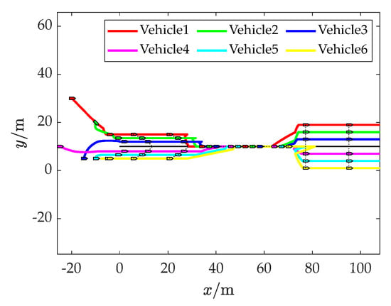
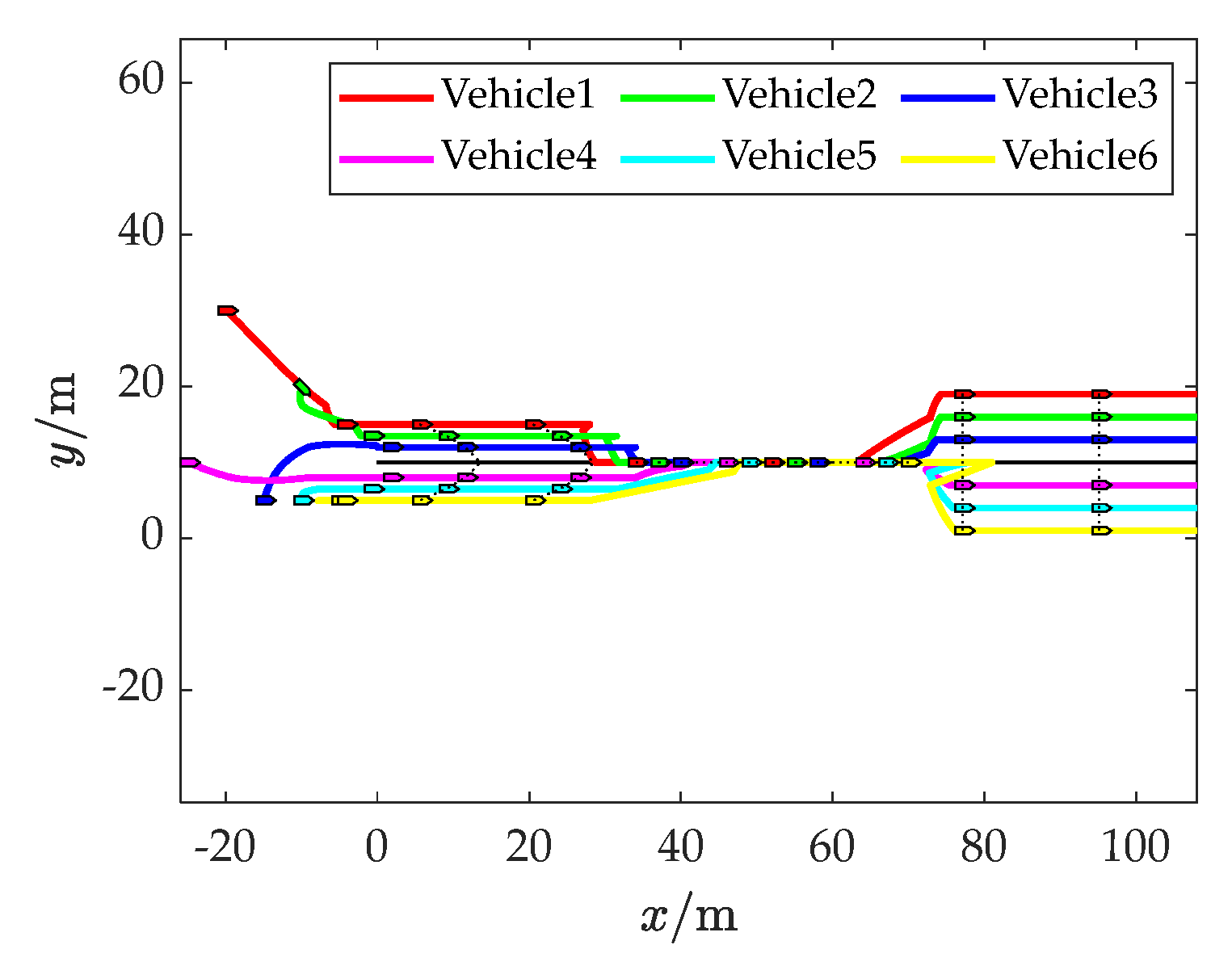
By using the proposed control law and adaptive law, the simulation results are depicted in Figure 1, Figure 2, Figure 3 and Figure 4. Figure 1 shows the trajectories of six vehicles on the plane, and it is obvious that the desired formation shape is finally obtained. Using the designed controller, all the closed-loop systems should be SGUUB.
Figure 1.
Formation trajectory on plane.
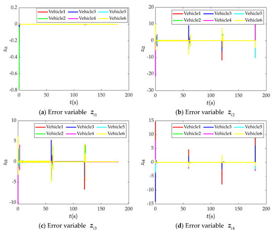
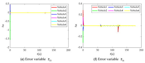
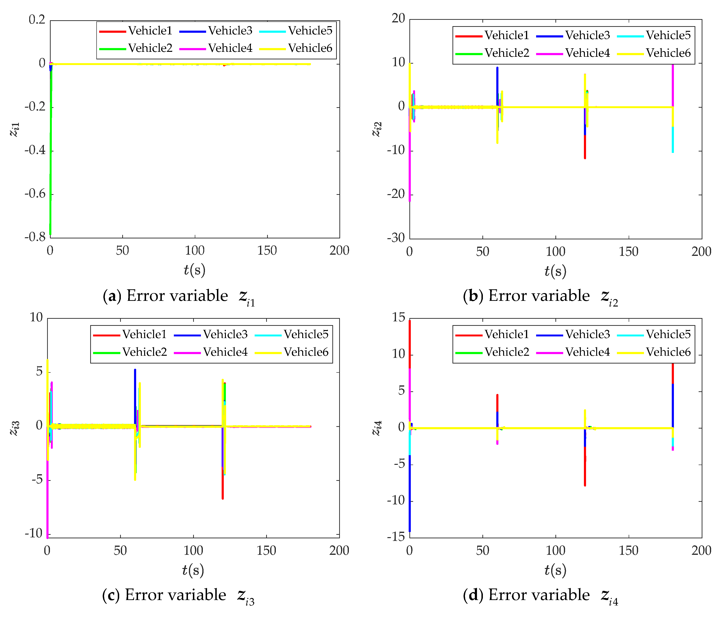
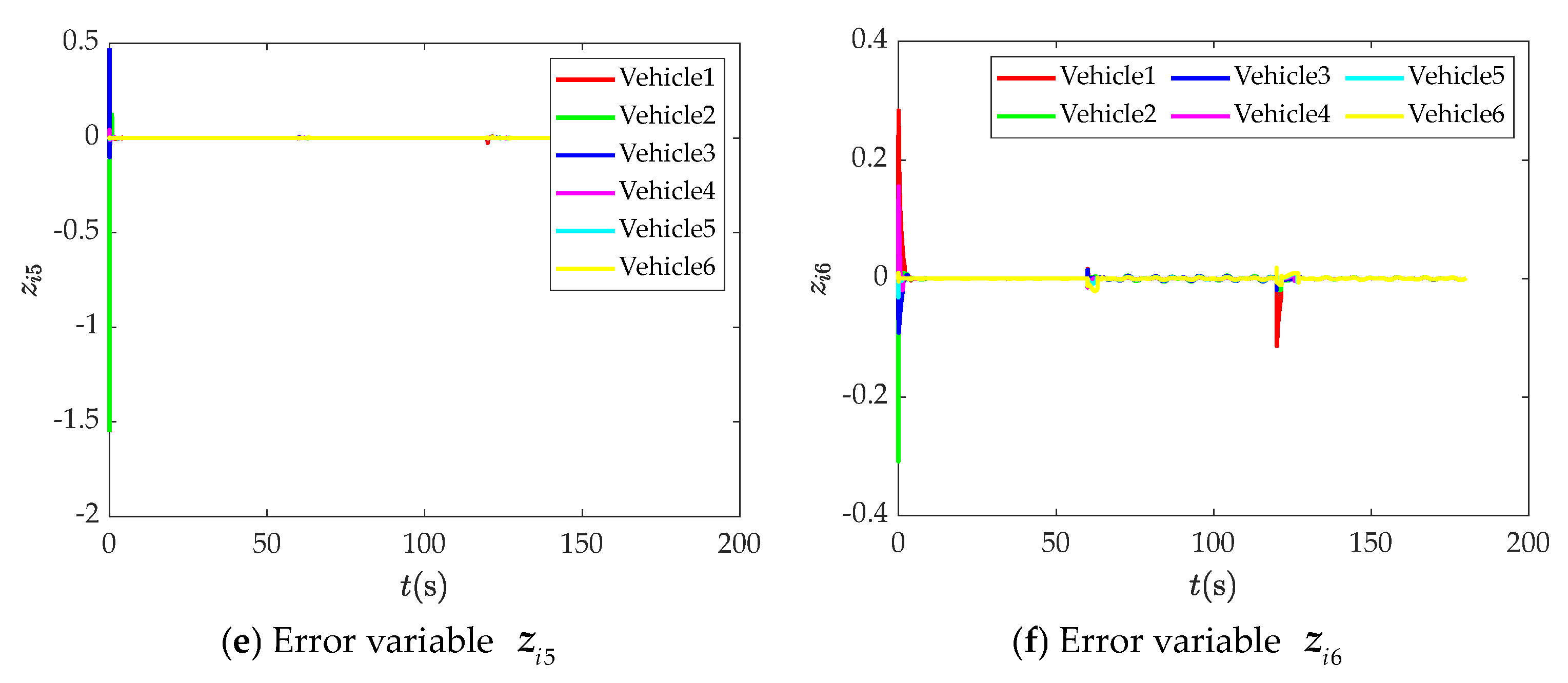
Figure 2.
Model error variables.
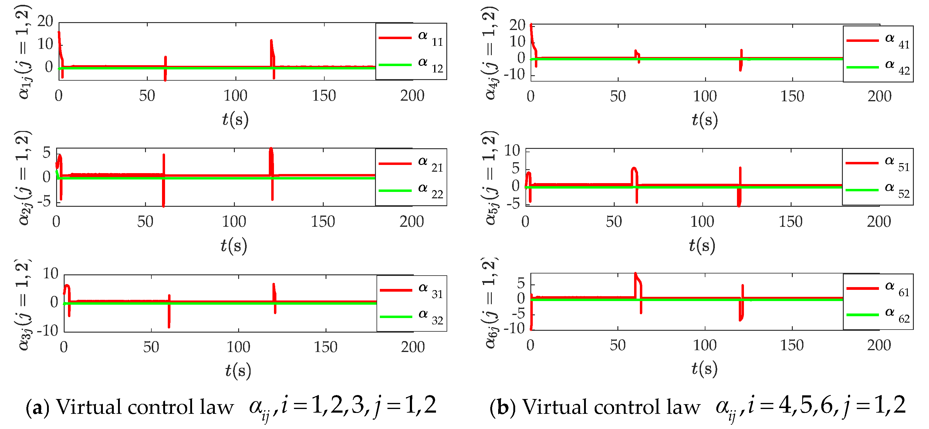
Figure 3.
Virtual control law.
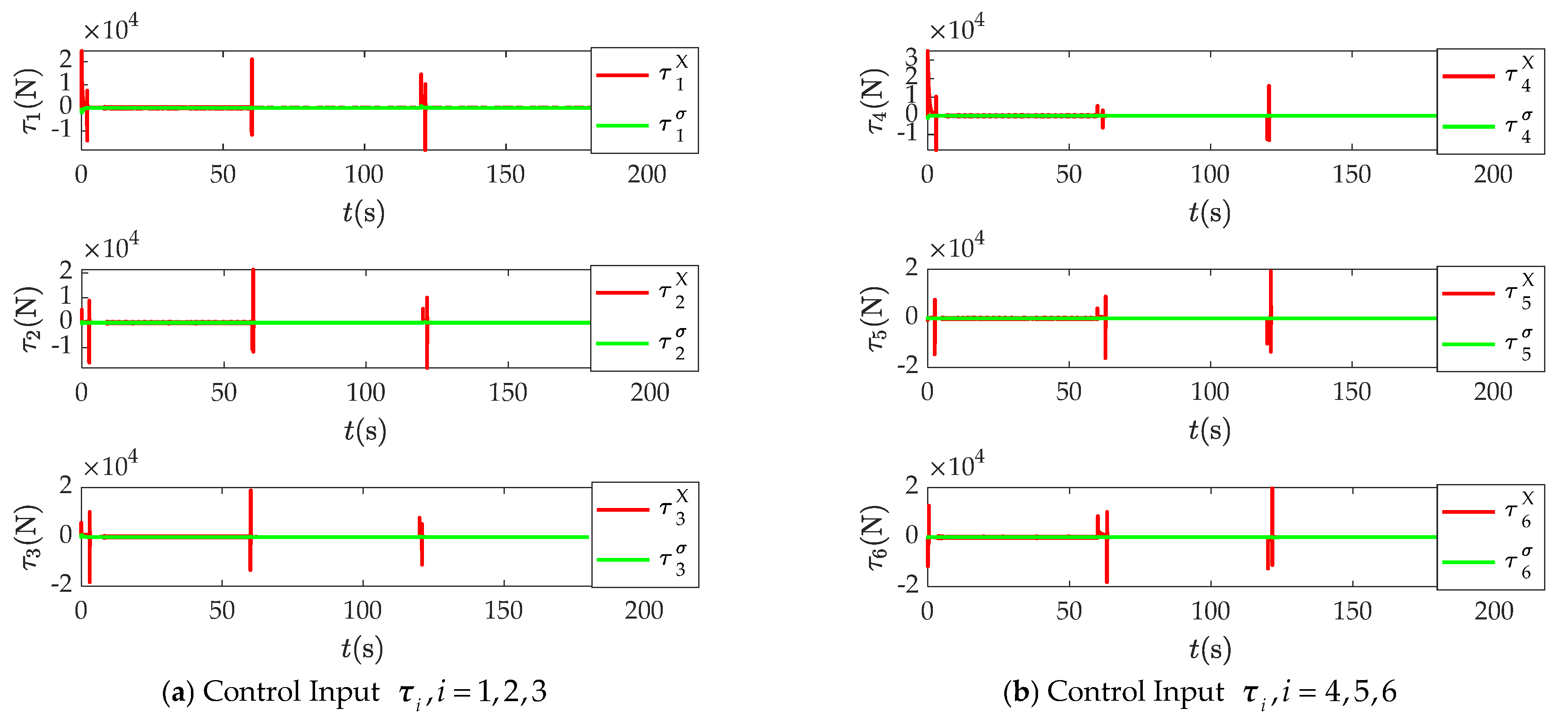
Figure 4.
Control Input.
Figure 2 shows the error variables of each vehicle. It is obvious that the chattering of the curve is less, and the error variables of the model are SGUUB.
The virtual control laws and of each vehicle are shown in Figure 3. We can observe that the control of the attitude subsystem and the position subsystem are continuous and SGUUB.
The control inputs and of each vehicle are shown in Figure 4. We can observe that the simulation curve of is relatively chattering-free, and all the controls of the position subsystem and attitude subsystem are continuous and SGUUB.
The above simulation results are consistent with Theorems 1 and 2.
5. Conclusions and Discussion
This paper presents a distributed adaptive formation control scheme for UUSV based on a directed graph. In the design process, considering the underactuation characteristics, we redefine the dynamic and kinematic models of the formation. The RBF neural network based on MLP is used for the online approximation of uncertain model parameters and external disturbances. DSC is used to solve the complex differential problem in the calculation process, which further improves the practicability of the controller. From the simulation results, it can be seen that the controller and two adaptive laws designed by this scheme successfully realize the effective control of the formation, achieve the desired goal, and effectively solve the underactuated control of UUSV formation and the uncertain problems of the dynamic model and quantitative parameters. In the future, we will carry out research on the event-triggered UUSV formation control technology.
Author Contributions
Conceptualization, W.H., L.Z. and X.C.; methodology, W.H. and Y.L.; software, W.H.; validation, Y.Z., L.Z. and Y.L.; formal analysis, Y.Z. and W.H.; investigation, L.Z.; resources, L.Z.; data curation, Y.Z.; writing—original draft preparation, W.H.; writing—review and editing, L.Z.; visualization, Y.Z.; supervision, Y.Z.; project administration, L.Z.; funding acquisition, L.Z. All authors have read and agreed to the published version of the manuscript.
Funding
This research was co-funded by the Fundamental Research Funds for the Central Universities grant number 3072024XX0108 and the National Key Research and Development Program of China grant number 2021YFC2803400.
Institutional Review Board Statement
Not applicable.
Informed Consent Statement
Not applicable.
Data Availability Statement
Data are unavailable due to privacy restrictions.
Conflicts of Interest
The authors declare no conflicts of interest.
References
- Zhang, L.; Zheng, Y.; Huang, B.; Su, Y. Finite-time trajectory tracking control for under-actuated unmanned surface vessels with saturation constraint. Ocean Eng. 2022, 249, 110745. [Google Scholar] [CrossRef] [Scilit]
- Zheng, Y.; Zhang, L. Internal model observer-based distributed moving-target-fencing control of multiple underactuated marine surface vehicles with intermittent communications. Ocean Eng. 2024, 300, 117383. [Google Scholar] [CrossRef] [Scilit]
- Zhang, L.; Zheng, Y.; Huang, Z.; Huang, B.; Su, Y. Distributed global output-feedback formation control without velocity measurement for multiple unmanned surface vehicles. ISA Trans. 2024, 147, 118–129. [Google Scholar] [CrossRef] [Scilit] [PubMed]
- Yan, C.; Zhang, W.; Su, H.; Li, X. Adaptive bipartite time-varying output formation control for multiagent systems on signed directed graphs. IEEE Trans. Cybern. 2021, 52, 8987–9000. [Google Scholar] [CrossRef] [Scilit]
- Wu, W.; Peng, Z.; Wang, D.; Liu, L.; Han, Q.-L. Network-based line-of-sight path tracking of underactuated unmanned surface vehicles with experiment results. IEEE Trans. Cybern. 2021, 52, 10937–10947. [Google Scholar] [CrossRef] [Scilit]
- He, S.; Wang, M.; Dai, S.-L.; Luo, F. Leader–follower formation control of USVs with prescribed performance and collision avoidance. IEEE Trans. Indust. Informat. 2018, 15, 572–581. [Google Scholar] [CrossRef] [Scilit]
- Peng, Z.; Wang, D.; Li, T.; Han, M. Output-feedback cooperative formation maneuvering of autonomous surface vehicles with connectivity preservation and collision avoidance. IEEE Trans. Cybern. 2019, 50, 2527–2535. [Google Scholar] [CrossRef] [Scilit]
- Zheng, Y.; Zhang, L.; Huang, B.; Su, Y. Distributed secure formation control for autonomous surface vessels by performance adjustable event-triggered mechanism. Int. J. Robust Nonlinear Control 2023, 33, 8490–8507. [Google Scholar] [CrossRef] [Scilit]
- Li, S.; Er, M.J.; Wang, N.; Chien, C.-J.; Yang, Z. Adaptive fuzzy output regulation for formation control of unmanned surface vehicles. In Proceedings of the 2017 International Conference on Fuzzy Theory and Its Applications, New York, NY, USA, 12–15 November 2017; pp. 1–6. [Google Scholar]
- Peng, Z.; Wang, J.; Wang, D. Distributed maneuvering of autonomous surface vehicles based on neurodynamic optimization and fuzzy approximation. IEEE Trans. Control Syst. Technol. 2018, 26, 1083–1090. [Google Scholar] [CrossRef] [Scilit]
- Peng, Z.; Wang, D.; Chen, Z.; Hu, X.; Lan, W. Adaptive dynamic surface control for formations of autonomous surface vehicles with uncertain dynamics. IEEE Trans. Control Syst. Technol. 2012, 21, 513–520. [Google Scholar] [CrossRef] [Scilit]
- Peng, Z.; Wang, D.; Li, T.; Wu, Z. Leaderless and leader-follower cooperative control of multiple marine surface vehicles with unknown dynamics. Nonlinear Dyn. 2013, 74, 95–106. [Google Scholar] [CrossRef] [Scilit]
- Zhao, Y.; Guo, G.; Ding, L.; Xu, Y.; Xu, H. Collision/obstacle avoidance control of vessel formation. Inf. Control. 2012, 41, 425–432, 438. [Google Scholar]
- He, S.; Dai, S.-L.; Luo, F. Asymptotic trajectory tracking control with guaranteed transient behavior for MSV with uncertain dynamics and external disturbances. IEEE Trans. Ind. Electron. 2018, 66, 3712–3720. [Google Scholar] [CrossRef] [Scilit]
- Chen, Y.; Wei, P. Coordinated adaptive control for coordinated path-following surface vessels with a time-invariant orbital velocity. IEEE/CAA J. Autom. Sin. 2014, 1, 337–346. [Google Scholar] [CrossRef] [Scilit]
- Jin, X. Fault tolerant finite-time leader-follower formation control for autonomous surface vessels with LOS range and angle constraints. Automatica 2016, 68, 228–236. [Google Scholar] [CrossRef] [Scilit]
- Riahifard, A.; Rostami, S.M.H.; Wang, J.; Kim, H.-J. Adaptive leader-follower formation control of under-actuated surface vessels with model uncertainties and input constraints. Appl. Sci. 2019, 9, 3901. [Google Scholar] [CrossRef] [Scilit]
- Qu, Y.; Cai, L. Nonlinear positioning control for underactuated unmanned surface vehicles in the presence of environmental disturbances. IEEE/ASME Trans. Mechatron. 2022, 27, 5381–5391. [Google Scholar] [CrossRef] [Scilit]
- Karnani, C.; Raza, S.A.; Asif, M.; Ilyas, M. Adaptive control algorithm for trajectory tracking of underactuated unmanned surface vehicle (UUSV). J. Robot. 2023, 2023, 4820479. [Google Scholar] [CrossRef] [Scilit]
- Mu, D.; Wang, G.; Fan, Y. Trajectory tracking control for underactuated unmanned surface vehicle subject to uncertain dynamics and input saturation. Neural Comput. Appl. 2021, 33, 12777–12789. [Google Scholar] [CrossRef] [Scilit]
- Li, S.; Wang, X. Finite-time consensus and collision avoidance control algorithms for multiple AUVs. Automatica 2013, 49, 3359–3367. [Google Scholar] [CrossRef] [Scilit]
- Lombana, D.A.B.; Di Bernardo, M. Multiplex PI control for consensus in networks of heterogeneous linear agents. Automatica 2016, 67, 310–320. [Google Scholar] [CrossRef] [Scilit]
- Ge, S.S.; Wang, C. Adaptive neural control of uncertain MIMO nonlinear systems. IEEE Trans. Neural Netw. 2004, 15, 674–692. [Google Scholar] [CrossRef] [Scilit] [PubMed]
- Skjetne, R.; Fossen, T.I.; Kokotović, P.V. Adaptive maneuvering, with experiments, for a model ship in a marine control laboratory. Automatica 2005, 41, 289–298. [Google Scholar] [CrossRef] [Scilit]

Disclaimer/Publisher’s Note: The statements, opinions and data contained in all publications are solely those of the individual author(s) and contributor(s) and not of MDPI and/or the editor(s). MDPI and/or the editor(s) disclaim responsibility for any injury to people or property resulting from any ideas, methods, instructions or products referred to in the content. |
© 2024 by the authors. Licensee MDPI, Basel, Switzerland. This article is an open access article distributed under the terms and conditions of the Creative Commons Attribution (CC BY) license (https://creativecommons.org/licenses/by/4.0/).