


Abstract
Understanding the role of faults in directing groundwater flow within bedrock aquifers is crucial, especially in the arid Southwestern United States, where water demand is exceptionally high. This study investigates the confined Coconino aquifer (Permian, 282–270 Ma), located between Springerville and Saint Johns, Arizona, and supplying the Springerville Generating Station. Using abundant well-pumping and water-level data, we analyzed how distinct regional geological structures, specifically the Coyote Wash fault (a steeply dipping normal fault; initially 70–30 Ma old with subsequent middle-to-late Quaternary and younger activity (<750 ka), the Cedar Mesa anticline, and the Buttes anticline, control local groundwater movement. Although the parallel Coyote Wash and Cedar Mesa structures experience similar regional stresses, model calibration yields hydraulic characteristics (hydraulic conductivity divided by barrier thickness) of 1.0 1/day for the Coyote Wash fault and 0.0001 1/day for the Cedar Mesa anticline, four orders of magnitude lower. Seismic reflection profiling reveals a disrupted zone, roughly 200 m wide, associated with the Cedar Mesa structures. Because these faults are perpendicular to the maximum horizontal stress direction, prevailing compressive forces theoretically close fracture apertures and severely restrict water flow. However, this study reveals that highly permeable regions exist where the structural damage zones of these prominent faults overlap. Ultimately, even in restrictive geological environments where ambient stresses predict sealed fractures, the overlapping damage zones of multiple intersecting faults can unexpectedly generate critical, highly permeable pathways for sustained deep groundwater flow today.
Keywords:
groundwater; MODFLOW; GMS; fault; anticline; Coconino aquifer; Little Colorado River; Lyman Lake; St. Johns; Arizona 1. Introduction
Groundwater is a critical resource whose importance is difficult to overstate. In the USA, for example, aquifers supply 37% of drinking water and 42% of irrigation water [1]. In this study, we examine the influence of adjacent normal faults and folds in a bedrock aquifer that governs large-scale groundwater movement, as well as the effects of pumping on that movement. The study was conducted in the arid Southwestern USA, a region that is highly dependent on groundwater resources. This area has also been affected by prolonged drought and long-term water withdrawals.
Faults are well known to influence water flow in bedrock aquifers, where fine-grained fault cores are often considered barriers to cross-fault flow [2,3,4,5,6,7,8], although some faults may switch between acting as barriers or conduits [9,10,11,12,13]. Fluid flow along or around faults also depends on bedrock lithology and the regional stress field. Near St. Johns and Springerville, Arizona (Figure 1), faults that dissect a major bedrock aquifer provide an opportunity to further examine the role of faults as conduits or barriers (or neither) to flow.
Figure 1.
Index map of the study area, showing the model domain outline, potentiometric contour elevations (cyan, m), and stress indicators (thick black arrows) [14]. The reader is referred to [6] for information on the source and uncertainty of the maximum horizontal stress orientation and how the stress direction was determined. Pumping wells are shown as green stars, water-level wells as black dots. Red lines indicate faults [12,15,16]. The two areas of geophysical surveys are indicated.
A major commercial groundwater user in eastern Arizona is the Springerville Generating Station (SGS), a coal-fired power plant owned and operated by Tucson Electric Power Company (TEPCO) [17]. Cooling and processing water for the plant is derived entirely from groundwater, and many production wells are located near two major structures: the steeply dipping Coyote Wash normal fault (initially 70–30 Ma old with subsequent middle-to-late Quaternary and younger activity (<750 ka [16]) and what has been called the Cedar Mesa anticline (Figure 1). The Cedar Mesa anticline formed primarily during the Laramide Orogeny roughly 75 to 55 Ma. As discussed below, this “anticline” also exhibits fault-like characteristics. Whether this structure is a fault, a fold, or both, its presence is evaluated based on its influence on groundwater flow. Consequently, the aquifer has responded to the hydraulic stresses imposed by long-term, high-volume pumping, making this site an ideal locality for investigating the role of faults in groundwater movement.
To assess the hydrological properties of these geologic structures, we have constructed a steady-state groundwater flow model. Ultimately, our goal was to improve understanding of the hydrological characteristics of faults, both with and without pumping, in a setting where damage-zone fractures should tend to be closed. This led to the following objectives:
- First, starting from a baseline model built with literature-based hydraulic properties (Section 3.3), calibrate the model to identify low- and high-permeability zones in the aquifer and examine permeability distributions relative to faults. Our study builds on previous hydrological modeling [18], discussed below.
- As part of the calibration process, determine whether the Cedar Mesa anticline axis acts as a horizontal barrier to flow. In other words, does it behave like a fault, and does this behavior differ from that of the Coyote Wash fault?
- Use particle tracking to examine likely flow pathways and flow rates in response to fault architecture and pumping.
- Turn off the wells and use particle tracking to examine the response of the flow field to the absence of pumping stresses, thereby providing additional insight into how groundwater flow responds to these faults.
- Use seismic reflection and ground-penetrating radar (GPR) to characterize fault architecture in relation to groundwater flow.
To achieve these goals, a model was developed to map the subsurface geology of the Springerville-St. Johns area, using borehole lithologic records and groundwater flow data, with particular attention to the interaction between flow, the Coyote Wash fault, and the Cedar Mesa anticline axis. Using this stratigraphy, we constructed a three-dimensional groundwater flow model to test the stated purpose and objectives.
Modeling has previously been conducted within the study area. Ref. [18] performed finite-element simulations to understand the upward flow of CO2 from a large subjacent reservoir (described below) into a regional aquifer supplying cooling and process water to the SGS facility. This study served as an analog for the potential failure of a carbon capture and storage reservoir. Accordingly, Ref. [18] was primarily concerned with the vertical movement of fluids into the aquifer. In contrast, we focus on horizontal water movement within the overlying aquifer at larger spatial scales, with and without pumping-induced stresses. To help constrain the subsurface geology and understand groundwater movement, we collected two seismic reflection profiles near the Cedar Mesa fault and one seismic reflection and one ground-penetrating radar profile across the Buttes fault (Figure 1).
2. Hydrogeological Setting
2.1. Regional Setting
The Springerville-St. Johns area in eastern Arizona lies near the southern edge of the Colorado Plateau [19] and north of the Basin and Range province, along the northeast-trending Jemez lineament [20]. This tectonically active, 50-km-wide lineament features normal, strike-slip, and en-echelon faults, alongside late Pliocene to Pleistocene volcanic fields (2.1 to 0.3 Ma old; [21,22]), including the Springerville volcanic field (Figure 1). Here, basaltic volcanism covers 3000 km2, comprising numerous cinder cones and large-volume lava flows [23,24].
The Concho fault bounds this field to the northeast (Figure 1) and forms the southwest edge of a structural depression holding over 250 km2 of spring tufa (450 ka to present) [16,19,24]. The depression’s northeast boundary is the Coyote Wash fault, a deep normal fault extending into the granitic basement [24,25]. Locally, this fault is poorly constrained due to limited surface exposure and extensive southern drainage development [16,24].
The groundwater model area is geologically complex, with several faults, some of which had middle-to-late Quaternary and younger activity, including the Cedar Mesa anticline, the Coyote Wash fault, and several subsidiary structures (Figure 1). It is also underlain by a CO2 reservoir [26,27,28], which includes travertine deposits [19,20,24,29]. The Coyote Wash fault and Cedar Mesa anticline play a significant role in the relationships among the St. Johns CO2 gas field, groundwater flow, and the travertine deposits. However, the interaction between these structures and their effect on horizontal groundwater movement remains poorly understood.
2.2. Cedar Mesa Anticline/Fault
The Cedar Mesa anticline, also known as the St. Johns Dome, is a broad, asymmetrical anticline spanning 1800 km2 and trending northwest (Figure 1). Its axis plunges to the northwest and southeast [25,30,31]. However, other studies have described the fold axis as a fault [18,20,32,33], based on borehole records [29] indicating offset at depth [18]. Recent groundwater-monitoring reports [34] for the SGS follow this interpretation. In addition, drilling and groundwater monitoring along the Cedar Mesa anticline in the SGS well field have revealed conditions suggesting that the hinge acts as a barrier to lateral groundwater flow and may offset strata [35]. Thus, this study treats the Cedar Mesa anticline as containing a fault core.
2.3. Hydrostratigraphy
The water-bearing strata of the model area are dominated by sedimentary rocks ranging in age from Pennsylvanian to Quaternary, although Jurassic rocks are absent (Figure 2). An unconformity separates these sedimentary rocks from the Precambrian granitic basement [30,36]. Groundwater occurs locally in Quaternary deposits; however, the primary aquifer (the Coconino aquifer, or C-aquifer) comprises highly fractured Kaibab Limestone and Coconino Sandstone (Permian, 282–270 Ma old), and, locally, the upper portions of the Supai Formation [25,36,37,38]. The Coconino Sandstone and Kaibab Limestone are hydraulically connected stratigraphically to their laterally equivalent units, the Glorieta Sandstone and San Andres Limestone. However, in this study, we retain the exclusive use of the Permian Coconino Sandstone and Kaibab Limestone. The C-aquifer underlies the model area and is a primary source of groundwater in northeastern Arizona [17,38].
Figure 2.
Stratigraphic column for the model area, indicating the hydrostratigraphic units included in the model. The column uses multiple colors for multiple stratigraphic units, in order to depict a hydrostratigraphic framework. Because there is no unique color to assign to the confining and confined aquifer layers, we have used a generic blue in contrast to other prominent strata such as volcanic rocks and tufa.
2.4. Surface Water
The primary perennial stream in the area is the Little Colorado River. The river is impounded between Springerville and St. Johns to form Lyman Lake (Figure 1) [39]. Downstream, flow now depends on releases from Lyman Lake and discharge from Salado Springs, located midway between Lyman Lake and St. Johns [40]. The potentiometric surface is shallow near St. Johns and Lyman Lake. Historically, groundwater has been discharged from the aquifer into the river and the C-aquifer reservoir [38].
2.5. Groundwater
The recharge areas for the C-aquifer for the model area lie to the south in the highlands of the Mogollon Rim [41]. The C-aquifer in the model area is part of the regional Little Colorado River Basin flow system. Recharge to the C-aquifer occurs almost entirely outside the model domain, on the higher terrain along the southern margin of the basin where the aquifer units crop out or are overlain by permeable surficial deposits [36,38,39]. Within the model area, the C-aquifer is orders of magnitude beneath the Chinle and Moenkopi Formations, and direct recharge from precipitation is negligible. Groundwater therefore enters the study area as lateral underflow from the south and southeast and moves northward toward the Little Colorado River, which historically gained water from the aquifer near Lyman Lake and St. Johns [36,38]. The steady-state model applies to all 14 SGS production wells simultaneously at the period-averaged rates in Table 1, a combined withdrawal of about 63,900 m3/day. The wells came into production between 1985 and 2017, so this total is the steady-state stress imposed on the model and does not correspond to withdrawals in any single year. In the model, this withdrawal is balanced by increased inflow across the southern boundary, reduced outflow across the northern boundary, and capture of groundwater that would otherwise have discharged to the Little Colorado River and Lyman Lake; the capture is reflected in the observed decline of flows in the river and the lake (Section 2.4).
Table 1.
Average pumping rate during active pumping intervals for production wells at the Springerville Generating Station.
The groundwater and surface springs near the Cedar Mesa anticline contain high levels of HCO3- (up to 1200 mg/L) due to the migration of dissolved CO2 from the St. Johns gas field [42,43]. The extensive travertine deposits in the area, particularly between Lyman Lake and Salado Springs, formed as CO2-enriched groundwater emerged from springs and rapidly precipitated calcium carbonate [24,26,42,44]. However, the outflow rate of CO2-enriched waters and the rate of travertine precipitation have declined significantly over time, likely due to a decline in hydraulic head and a lowering of the water table [24,36,45].
2.6. CO2 Reservoir
Although this study focuses primarily on horizontal water movement within the C aquifer, it is important to note the presence of the subjacent CO2 reservoir. Within the Cedar Mesa anticline, the Supai Formation and fractured Precambrian granite locally form a CO2 gas deposit (Figure 2; [46]). The reservoir is relatively shallow, 200–700 m below the surface, with an average depth of 600 m [31,45]. The antiformal structure and overlying clays, mudstones, and anhydrite beds create a seal [30,46]. The gas occurs in discontinuous, vertically isolated reservoirs separated by thin impermeable beds [24,31]. An estimated 393 billion m3 of CO2 exists as free gas in the reservoir [21]. Although CO2 is the primary gas (average of 92%), nitrogen (6.6%), helium (0.6%), and argon (0.2%) also occur. The concentrations of these gases vary spatially within the dome. Based on helium-isotope compositions, the CO2 was derived from a mix of crustal and magmatic sources, with up to 20% of the helium originating from the mantle [27,45].
CO2 has recently leaked to the surface [12]. Travertine deposits indicate that the Coyote Wash fault zone is the primary pathway for CO2 transport to the surface [16,20,45]. Additionally, 3He/4He ratios measured along the Coyote Wash fault and at its northern tip near Salado Springs indicate the transport and mixing of magmatically derived CO2 and noble gases typically found only at depth [43]. This suggests that upward transmission of CO2 likely occurs along the damage zone [38,43,47].
2.7. Structural Control
The Coyote Wash fault and Cedar Mesa anticline have a significant yet incompletely understood role in the relationships among the St. Johns gas field, groundwater flow, and the travertine deposits. The SGS has several groundwater production wells in the Coyote Wash fault zone. On the downthrown, southwest side of the fault, these wells have high yields and minimal drawdown [18]. The upthrown, northeast side of the fault is thought to be a hydrologically distinct zone, where wells also experience minimal measurable drawdown, but the Kaibab Limestone portion of the C-aquifer is dry on the east side of the fault [18,32]. Measurements [14] suggest that maximum horizontal compressive stresses are oriented NNE-SSW to N-S (Figure 1), indicating that fractures may be open in these orientations, but are less likely in ESE-WNW-oriented fractures within damage zones of structures such as the Coyote Wash fault and Cedar Mesa anticline because Mode I open (tensile) fractures form perpendicular to the minimum principal compressive stress. The subsurface significance is that parallel-striking open fractures typically act as primary fluid pathways and critically stressed conduits in deformed or fractured reservoirs.
3. Methods
The three-dimensional steady-state groundwater model was developed for the study area using the United States Geological Survey MODFLOW modular groundwater flow code [48], in its MODFLOW-NWT Newton formulation (Section 3.3). The Groundwater Modeling System software, version 10.4.6 [49,50], was used for model construction, calibration, and pre- and post-processing. A detailed description of the modelling methods is provided in [51], including particle-tracking calculations to evaluate the influence of the Coyote Wash fault and Cedar Mesa anticline on groundwater movement. We summarize the methods here to provide the necessary context for the rest of the manuscript.
3.1. Model Conceptualization and Data Sources
Model boundary conditions were defined as general-head boundaries on the north and south, and no-flow boundaries on the east and west. General-head boundaries assume that water flows across the boundary driven by head differences, whereas no-flow boundaries were oriented perpendicular to potentiometric surface contours (parallel to flow directions). This study relied heavily on available subsurface data [40], as well as on geophysical surveys (Figure 3). The Coyote Wash fault and the Cedar Mesa anticline axis were digitized based on their locations in [40]. We interpret the C-aquifer in the study area as confined. In the comprehensive study by [41], their much larger model domain is split into areas where the C-aquifer is confined and unconfined. The base of the Moenkopi Formation (Figure 2) is used to define the confining unit in our study. Ref. [41] defines unconfined as areas where the potentiometric surface is below the base of the Moenkopi. We have defined the confined aquifer as everywhere where the Moenkopi and other fine-grained Mesozoic rocks are present. Thus, recharge occurs externally and flows into the model domain along the south-southeastern general-head boundary.
Figure 3.
Map of the model domain and grid, including faults, the well, surface water, and potentiometric contours, as described in Figure 1. Green contours represent the output of the steady-state calibrated model. Areas of geophysical surveys are indicated. See Figure 2 for explanations of other symbols.
The Little Colorado River and Lyman Lake are the primary surface water bodies within the study area. Historically, both the river and the lake were gaining [36,52]. However, declines in the potentiometric surface of the confined C-aquifer, caused by pumping, have reduced flows in both the Little Colorado River and Lyman Lake. The model accounts for any resulting recharge from surface water.
The power plant has 14 active pumping wells in the study area (Figure 1 and Figure 3). Locations and borehole logs for these wells and others on the SGS property were provided by [34,40]. Additional borehole data, including approximate locations within the study area, were obtained from the Arizona Department of Water Resources [53] Registry of Wells in Arizona (Wells 55) database and digitized according to TEP internal monitoring reports or the ADWR Wells 55 registry. Well locations were further refined using tax parcel information and aerial imagery.
3.2. Three-Dimensional Hydrostratigraphy Model
As part of the model conceptualization process, a three-dimensional solid model of the conceptual hydrostratigraphy of the study area was constructed from digital elevation data and borehole logs. Digital elevation model (DEM) data were obtained from the [54] 3D Elevation Program at a resolution of 1/3 arc-second. The surface elevations of wells and boreholes were derived from the USGS DEM. The DEM was also used as the ground surface to which all geologic contacts were referenced.
A total of 42 borehole records were compiled and analysed to define the generalized subsurface hydrostratigraphy shown in Figure 2. Five units were identified from drill logs: (1) alluvium/Cenozoic deposits, (2) the Chinle and Moenkopi Formations, (3) the Kaibab Limestone, (4) the Coconino Sandstone, and (5) the Supai Formation. This stratigraphy was then simplified into two layers for the hydrostratigraphy model. The upper layer (units 1 and 2) comprises fine-grained, impermeable sediments and was implemented in the model as an aquitard, referred to as the “upper confining unit”. The hydrostratigraphy is summarized in Figure 2.
As noted above, the Kaibab Limestone, Coconino Sandstone and the upper portion of the Supai Formation comprise the C-aquifer, which forms the lower layer in the model. These three units were combined because they behave as a single hydraulically connected producing interval at the scale of the model: they are in direct contact, they are treated as one hydrostratigraphic unit in regional studies of the C-aquifer [36,38], and the available water-level data do not resolve vertical head gradients within them. Subdividing the C-aquifer would therefore have introduced layers that the observations could not constrain, without improving the representation of the horizontal and cross-fault flow that is the subject of this study.
Examination of borehole records within the model indicates that the Kaibab Limestone and Coconino Sandstone are largely consistent in thickness across the study area [36,39], albeit deformed and offset by the Coyote Wash and Cedar Mesa structures. For boreholes where drilling did not penetrate the full thickness of the C aquifer, the missing lower contacts were filled by the same inverse-distance-weighted interpolation used to build the solid model, preventing artificial truncation of aquifer thicknesses. Those boreholes therefore contribute no independent control on the base of the C-aquifer, which is constrained by the fully penetrating boreholes. The upper 40 m of the Supai Formation was included in the C aquifer. Deeper, the Supai Group grades into impermeable siltstone and evaporite deposits [39]. Elevations of borehole contacts were then spatially interpolated using an inverse distance-weighted algorithm to generate a three-dimensional solid model of the subsurface. Inverse-distance weighting is the interpolation scheme used by the borehole-to-solid workflow in GMS [49,50], and it suits the available data: it is an exact interpolator that honors the measured contact elevations, it requires no variogram model, which the 42 irregularly distributed boreholes are too few to constrain reliably, and it does not impose a regional trend beyond the data. The Kaibab Limestone and Coconino Sandstone contacts vary gently across most of the model area, so the choice of interpolation scheme has limited leverage on the resulting surfaces. Where the units are offset across the Coyote Wash fault and the Cedar Mesa anticline, any smoothly varying interpolator will smear the offset; the hydraulic effect of these structures is therefore imposed explicitly through the Horizontal Flow Barrier package (Section 3.3) rather than through layer geometry. An alternative interpolator was not available within this workflow, so no formal comparison was performed, and the hydrostratigraphic geometry accordingly remains a source of model uncertainty. The conclusions of the study, however, do not rest on the interpolated geometry. Where the units are offset across the Coyote Wash fault and the Cedar Mesa anticline, any smoothly varying interpolator smears the offset; the hydraulic behavior of these structures is imposed through the Horizontal Flow Barrier package and calibrated against head observations, independently of the layer geometry. A different interpolator would produce slightly different layer elevations but would not change the calibrated conductivity contrast between the two structures, which is the central result.
The hydrostratigraphic solid model was constructed entirely from the DEM and the 42 borehole records and was not fitted to an independent subsurface dataset. Interpolated unit thicknesses were checked for continuity and for consistency with the regional hydrostratigraphy reported by [36,39], and the ability of the calibrated flow model to reproduce observed heads provides an indirect test of the geometry. Neither check constitutes independent validation: the high-resolution seismic profiles described in Section 4.3 image the shallow subsurface and were not used to constrain unit contacts. Away from the boreholes, the geometry of the hydrostratigraphic units therefore remains a source of model uncertainty.
3.3. Numerical Model
A steady-state MODFLOW groundwater model for the study area was developed. The model comprised two layers corresponding to the two primary hydrostratigraphic units, and the top and bottom elevations for the grid cells in each layer were derived from the solid model. The resulting two-layer 3D grid was rotated to align with the northwest strike of the Coyote Wash fault and Cedar Mesa anticline (Figure 3), facilitating testing of the structures as linear hydraulic flow barriers. The C-aquifer is confined throughout the model domain and does not by itself require a Newton formulation. The overlying confining unit, however, is largely unsaturated, so cells within it dry and rewet during the iterative solution; in the standard MODFLOW formulation, such cells are deactivated, which commonly produces convergence failures. MODFLOW- [55] was used because its Newton-Raphson formulation treats cell drying as a continuous process and converges reliably under these conditions. The solver choice affects numerical stability in the upper layer and does not alter the confined representation of the C-aquifer.
General head boundaries (Figure 3) were implemented using the MODFLOW General Head Boundary (GHB) package. Head values were estimated from observed heads at nearby observation points. The north boundary was assigned a uniform starting head of 1615 m, whereas the south boundary was assigned a starting head of 1870 m at the west edge, 1900 m at the intersection with the Coyote Wash fault, and 1967 m east of the Cedar Mesa anticline. Conductance for both the north and south general head boundaries was set to 1 m2/day/m. These starting heads were obtained by projecting the observed potentiometric surface (Figure 1) onto the model boundaries using the nearest water-level observations; the south boundary was subdivided at the Coyote Wash fault and the Cedar Mesa anticline because the potentiometric surface is offset across those structures. Boundary heads and conductances were then adjusted during calibration together with the hydraulic conductivity fields (Section 3.4), so the values reported here are calibrated effective boundary conditions rather than fixed measurements. Their uncertainty was addressed through this calibration rather than by a formal uncertainty analysis, which was not performed. Because both general-head boundaries lie well outside the well field and the two structures, residual error in the boundary heads is largely absorbed by the calibrated conductivity field and has limited influence on the head loss across the barriers, from which the fault hydraulic characteristics are derived.
For the faults, the MODFLOW Horizontal Flow Barrier (HFB) package was used to create a partial horizontal barrier to flow along vertical grid-cell walls most closely aligned with the Coyote Wash fault and the Cedar Mesa anticline (Figure 3). MODFLOW characterizes such a barrier by its hydraulic characteristic, the hydraulic conductivity of the barrier material (K, m/day) divided by the horizontal thickness of the barrier normal to flow (T, m), which therefore has units of 1/day. The specific discharge across the barrier (q, m/day) is the product of this hydraulic characteristic and the head drop across the barrier (∆H, m) [56]:
The barrier is applied to a vertical cell face of area A (m2), so the volumetric flow across that face is Q = qA = (K/T)A∆H, with units of m3/day. In MODFLOW, the quantity (K/T)A is the barrier conductance (m2/day), which the solver multiplies by the head difference between the two adjacent cells to obtain the flow across the barrier. The model input is the hydraulic characteristic K/T; K and T are not specified separately, so the calibration constrains their ratio rather than either quantity alone.
The hydraulic characteristic for both the Coyote Wash fault and the Cedar Mesa anticline was initially set at 0.00001 1/day, based on the hypothesis that both acted as barriers to lateral flow.
To represent the hydrostratigraphic units, the initial K values were selected based on recommendations in [57]. For the confining layer, a value of 0.0001 m/d was chosen, reflecting the presence of fine-grained clastic sediments of the Chinle and Moenkopi Formations. For the C-aquifer, a value of 5.0 m/d was selected, reflecting the presence of fractured carbonate rocks and sandstone. These values were initially applied uniformly across both layers and were subsequently varied locally to calibrate the model. Together with the starting boundary heads and conductances given above and the initial river- and lake-bed conductances given below, these values define the baseline model that was run before calibration. Calibration then adjusted the hydraulic conductivity fields, the boundary heads and conductances, and the hydraulic characteristics of the two structures, as described in Section 3.4.
To estimate recharge into the model domain, the recharge package and parameter estimation techniques were employed in MODFLOW during calibration. Refs. [36,39] indicate that most recharge occurs where C-aquifer units are exposed at the surface, or in areas with more permeable surficial layers that lack the impermeable beds of the Chinle and Moenkopi Formations, allowing precipitation to percolate downwards. However, such areas lie outside the model domain, and groundwater instead enters the model as lateral underflow across the southern general-head boundary (Section 2.5).
The Little Colorado River was simulated using the MODFLOW River package, which requires river stage and bottom elevation for the cells representing the river in the model. The stream was divided into two segments, upstream and downstream of Lyman Lake (Figure 1). Stage elevations along the Little Colorado River were based on the available average stream-gage height for the recorded years. As the outflow from Lyman Lake lacks a stream gage, elevations were estimated using the outlet ground elevation as a starting point. There is a downstream gage for the Little Colorado River above Zion Reservoir, which lies outside Figure 1. Stream elevations were interpolated between these endpoints. A point at the boundary edge was then selected, and a model-generated head value was used. The stream-bottom elevation was estimated to be 5.18 m lower, based on measurements at the Little Colorado River Dam site, which is also located downstream [58].
Cell conductance (Ccell) for the river segments was calculated using the following formula [59]:
where K is the hydraulic conductivity of the riverbed material, W is the stream width, L is the length of the stream segment overlapping each cell (automatically calculated by GMS), and T is the vertical thickness of the riverbed sediments. The thickness of the riverbed sediments, T, was set to 5.2 m [58]. Ref. [58]’s report also established that the river-bottom sediments were predominantly wet clay; therefore, a K of 8.7 × 10⁻⁷ m/d was used to calculate the estimated starting values. Aerial imagery showed the stream to be an average of 7 m wide above Lyman Lake and 4 m wide below. Thus, upstream conductance values were estimated to be 1.16 × 10⁻⁶ m2/day/m and 6.66 × 10⁻⁷ m2/day/m downstream of Lyman Lake.
Lyman Lake was incorporated into the model using the MODFLOW General Head Boundary (GHB) package (Figure 1 and Figure 3). For the general head cells, Ccell is calculated as:
where K is the hydraulic conductivity of the lake-bottom sediments, T is the vertical thickness of the sediments, and A is the area of the cell (automatically calculated by GMS). Ccell values were also based on wet clay, using the thicknesses of riverbed sediments reported in [58], yielding an initial conductance of 1.67 × 10⁻⁷ m2/d/m2. Gage data were available for Lyman Lake for water years 1991–2009, 2018, and 2019. The average elevation during this period was 1816 m and was used in the model.
Pumping data for the SGS production wells were available for 1985–2018 [29]. Not all wells were in production throughout the entire period. The pumping rate for each well was averaged over its years of operation (Table 1). These averaged rates were then added to the model as extraction wells (Figure 1 and Figure 3).
3.4. Model Calibration
The model was calibrated using groundwater levels from 46 monitoring wells, measured in January 2019 and published in the [40] hydrogeologic monitoring program report, and entered as observation points across the model (Figure 1 and Figure 3). The calibration process was iterative until the model-generated head values aligned with the observed head values (Figure 4). Simulation results indicated that the river was not directly connected to the primary aquifer; thus, observed river-flow data (stream-aquifer discharge rates) were excluded as calibration targets.
Figure 4.
Plot of calculated versus observed heads from model calibration.
The head and conductance values assigned to the general head boundaries on the north, south, and southeast were iteratively refined during calibration. The hydraulic characteristics of both the Coyote Wash fault and the Cedar Mesa anticline were determined by iteratively adjusting that parameter in Equation (1) until the modelled head loss across the barrier matched the field-measured head loss.
To calibrate the cell hydraulic conductivity values, the confining unit and C-aquifer were each divided into two zones, based on the model response during calibration. Within each zone, a set of pilot points with specified minimum and maximum values was used to calibrate the aquifer’s hydraulic conductivity. A pilot point is a location at which a hydraulic conductivity value is assigned, and the hydraulic conductivity values for adjacent cells are obtained by spatial interpolation from these points. The area between the Coyote Wash fault and the Cedar Mesa anticline axis, or overlapping fault zone, contained 50 pilot points. Outside the fault zone, 41 pilot points were created. The values for these points were then adjusted and re-interpolated to the grid cells via inverse model runs with parameter estimation. Using two sets of pilot points enabled representation of the anisotropy introduced by faulting. The two sets differ in density because their counts emerged from the calibration rather than from a predetermined design. Points were added iteratively in each zone where the model could not reproduce the observed heads without additional local flexibility, and were left unchanged where it could. The area between the two structures required the denser set of 50 points, which reflects the greater short-wavelength variation in hydraulic conductivity there; the much larger area outside the structures was matched with 41 more widely spaced points. Calibrated values at all points were confined within specified minimum and maximum bounds. We did not carry out a formal parameter-identifiability or regularization analysis, so the individual point values should be read as one plausible realization of a smoothly varying conductivity field rather than as uniquely determined local measurements.
Initial model runs indicated that the conductance of the Little Colorado River bottom sediment was set too low. In response, a K of 0.03 m/d and a river-bed sediment thickness of 2 m were used to calculate an upstream conductance of 0.1042 m2/day/m and a downstream conductance of 0.0599 m2/day/m. Similarly, the K and thickness of the lake-bottom sediments appeared to be far too low and too thick, respectively. Ultimately, a conductance of 0.00009 m2/day/m was adopted.
3.5. Simulations
Because complete groundwater-monitoring data were available for only a single time period, the model was run as a steady-state simulation. Subsequently, simulations were run to examine the aquifer’s response with all pumping wells deactivated, allowing the behavior of groundwater flow relative to the faults to be explored both with and without active pumping. Both sets of simulations were visualized using particle tracking.
Once the groundwater model was fully calibrated, particle tracking was simulated using the USGS MODPATH model [60]. This model enables a more detailed examination of how hypothetical particles might move through a flow field under simple advection. It generates pathlines indicating groundwater flow directions (either forward or backward) and travel-time estimates. Travel times were converted from model-generated Darcy velocity to actual seepage velocity by scaling with an effective porosity value defined for each model cell. Because particles cannot be tracked through dry cells, cells in the upper confining unit that were dry in the calibrated model were inactivated for particle tracking; saturated parts of the upper unit remained active, and particles could enter and terminate within them. Since the upper unit is poorly connected to the C-aquifer over most of the model domain, this had little effect on the results. The effective porosity of the C-aquifer was set at 17.5% based on experimental results for Coconino Sandstone [61], with similar values reported by others [62,63]. The effective porosity of the C-aquifer was set at 17.5% based on experimental results for Coconino Sandstone [61], with similar values reported by others [62,63]. Effective porosity enters the particle-tracking calculation only through the conversion from Darcy flux to seepage velocity. It does not affect the calibrated steady-state head distribution, the flow directions, or the geometry of the pathlines, and travel times scale inversely with it. Reported travel times therefore rescale by a factor of n/0.175 for any alternative effective porosity n. Over a plausible range for the Coconino Sandstone of 10% to 25%, the C-aquifer travel times of ~790–1400 a reported below become ~450–800 a and ~1130–2000 a, respectively. In the fixed-duration 37-a case, porosity instead controls the distance travelled: at n = 10% particles would advance approximately 1.75 times as far as reported. Pathline geometry and the inferred role of the two structures are unaffected by this parameter, because both follow from the calibrated head field and the hydraulic characteristics assigned to the barriers.
Three particle-tracking simulation cases were used to examine behavior across the Cedar Mountain anticline and then across the Coyote Wash fault. Simulations were conducted under pumping conditions (case 1) or with pumping active and then shut off (cases 2 and 3). Case (1) included 20 particles placed around each of the 14 extraction wells. Particles were tracked both without a time limit and with a time limit of 13,514 days, or 37 years. This interval approximates the elapsed time since production began in 1985. It does not reproduce the pumping record: the model is steady state, and each well is applied continuously at the rate averaged over its own operating interval within the 1985–2018 record (Table 1), so wells that came into production later are treated as though they had operated throughout. The 37-year limit is therefore an elapsed-time cutoff applied to the calibrated steady-state flow field, and it indicates how far particles travel in that field over a period comparable to the production history. Case (2) included 18 particles generated within 30 cells located in the eastern half of the model area east of the Cedar Mesa anticline. These locations were chosen to examine the effects of fault properties with and without pumping stress. Case (3) included 18 particles generated within 20 cells that lie between the two structures under both pumping and non-pumping conditions. This approach permits evaluation of each structure as a potential barrier or conduit to flow.
3.6. Seismic Reflection and GPR Surveys
To guide the interpretation of shallow surface structure and stratigraphy, we acquired three high-resolution seismic compressional (P) wave common-midpoint (CMP) reflection profiles (Figure 1, Figure 3 and Figure 5). Two seismic CMP profiles were surveyed along the TEPCO access road over previously mapped or suspected faults (Figure 5). A partially coincident seismic reflection and ground-penetrating radar (GPR) profile (Figure 1 and Figure 3) was also acquired north of the TEPCO access road, crossing a series of travertine tufa mounds (Figure 1 and Figure 3). The locations of the seismic reflection profiles were constrained in part by logistical and permit issues. The west profile was surveyed so as to intersect the probable south-eastward extension of the Cedar Mesa fault/anticline (Figure 5). The east profile does not cross any previously mapped geologic faults or folds; however, it lies over a mapped tufa/travertine deposit (Figure 5), which may conceal deeper geological structures that could affect groundwater flow.
The two seismic profiles along the TEPCO access road were recorded using 96 channels (4.5-Hz vertical geophones), receiver and source spacings of 10 ft (3.05 m), a sample rate of 0.5 ms, a recording time of 3000 ms, and a Bison 500-lb (227-kg) elastic-wave generator. The seismic CMP profile over the tufa mounds (Figure 1 and Figure 3) was collected with 72 channels (4.5-Hz vertical geophones), a field filter of 10–500 Hz, receiver and source spacings of 10 ft (3.05 m), a sample rate of 0.5 ms, a recording time of 3000 ms, and a 16-lb (7.3-kg) sledgehammer stacked twice. The GPR profile was collected using a GSSI 200-MHz bistatic antenna in continuous mode. The recording time was 150 ns, the sample rate was 0.30 ns/trace, and the spatial sampling was 6 traces/ft (19.69 traces/m).
Data processing of geophysical profiles followed a standard sequence of steps. Processing of the seismic CMP profile over the tufa mounds (Figure 1 and Figure 3) included assignment of 3D geometry, top-muting of direct head-wave arrivals, bottom-muting of surface waves, an Ormsby bandpass filter of 20-45-200-400 Hz, automatic gain control (500-ms window), elevation static corrections using a replacement velocity of 800 m/s and a datum of 1920 m above sea level, normal move-out correction, CMP stack, adjacent-trace mixing to reduce the effect of low-apparent-velocity noise, phase-shift time migration, and time-to-depth conversion. The western seismic CMP profile along the TEPCO access road (Figure 5) followed a similar processing sequence, except that top-muting was applied with a CMP stretch mute of 30% (arrivals stretching beyond this were muted), followed by a bandpass filter of 35-60-200-400 Hz, and elevation static correction with a 2000 m/s replacement velocity and a datum of 2120 m above sea level. The eastern profile along the access road, on the eastern side of the fault (Figure 5), was processed similarly but was affected by aliased surface-wave noise. To mitigate this, we applied a bandpass filter of 45-700-200-400 Hz (biased against lower frequencies) and an adaptive deconvolution inverse filter with an operator length of 60 ms and a prediction “distance” of 30 ms. Further details on seismic CMP and GPR data processing techniques can be found in [64,65,66]. Because the GPR data are essentially single-channel, the processing stream was much simpler. The critical processing steps were “background” removal (attenuation of the direct arrival and ringdown), followed by exponential gain balancing, automatic gain control, application of a high-pass filter at 150 MHz and a low-pass filter at 310 MHz, adjacent-trace mixing, phase-shift migration, depth conversion, and topographic correction using a dielectric constant of 7, typical for limestone [67].
4. Results
4.1. Model Results
Model calibration results are presented in Figure 4. Of the 46 wells, all but three produced modelled water levels within 3 m of the observed values, with two showing differences of 3–6 m and one exceeding 6 m. The regression R2 is 0.9982. The mean residual, mean absolute residual, and root mean square residual heads (m) were 0.18, 1.17, and 1.95, respectively. A complete description of conductances, hydraulic conductivities, and boundary heads for the calibrated model is provided in [51].
The calibration process produced two outputs that were important for understanding the role of the structures in controlling groundwater flow in the C aquifer: (a) the distribution of K values in cells near the faults, and (b) the hydraulic characteristics assigned to the faults themselves. There is also an area of higher K values to the southwest of the central Coyote Wash fault (Figure 6). More broadly, calibration within the C aquifer required modestly higher hydraulic conductivities in areas adjacent to the southwestern and northeastern margins of the model domain. Calibration yielded hydraulic characteristics of 1.0 1/day for the Coyote Wash fault and 0.0001 1/day for the Cedar Mesa anticline [51]. These are calibrated effective parameters of the Horizontal Flow Barrier representation, obtained by adjusting the hydraulic characteristic in Equation (1) until the modelled head loss across each structure matched the observed head loss (Section 3.4); they are not direct field measurements of fault-rock properties. Because the hydraulic characteristic is the ratio K/T, the head observations constrain the across-strike hydraulic conductivity of each structure only in combination with its barrier thickness. The two values are directly comparable to one another: for a common barrier thickness, their ratio equals the ratio of the across-strike hydraulic conductivities of the two structures. Model calibration required only modest variations, with otherwise low K values in the upper confining layer.
Figure 6.
Distribution of hydraulic conductivities, K, for the upper confining layer and the C aquifer.
4.2. Particle Tracking
4.2.1. Case (1)
When allowed to run under present-day pumping conditions with no time limit, a reverse particle-tracking analysis starting at the wells indicates that ~2/3 of the particles reaching the wells originate in the confining layer (Figure 7), most of which originate in the Little Colorado River and Lyman Lake. Travel times through the confining layer ranged up to ~3200 a. The remaining ~1/3 of particles originated in the C-aquifer, with travel times ranging from ~1400 to ~790 a. Given these large model time periods, particle paths cross both the Coyote Wash fault and the Cedar Mesa anticline.
Figure 7.
Upper panel: Particle tracking towards production wells with no time limit in the model. Water may flow within both model layers. Lower panel: Particle tracking for the 37-a duration of pumping. All water flows within the C-aquifer towards the wells. A—A’ is a cross-section of particle tracks.
When the particle-tracking duration was shortened to 37 a, all particles originated within the C-aquifer (Figure 7). Regionally, the majority (80%) of particles started upgradient of the wells at a higher elevation and were drawn into the wells, whereas the remaining 20% started downgradient of the wells at a lower elevation and were captured by the cones of depression generated by pumping. A 37-a pumping duration was insufficient to draw any water across the Cedar Mesa anticline, but some wells near the Coyote Wash fault appear to have drawn water across it.
4.2.2. Case (2)
In this case, a set of particles was placed between the Coyote Wash fault and the Cedar Mesa anticline and tracked forward in time. Thus, this simulation examined the properties of the Coyote Wash fault under pumping and non-pumping conditions (Figure 8). Under pumping conditions, essentially all particles remained in the C-aquifer. With pumping shut off, ~one half of the particles terminated in the upper layer, discharging into the Little Colorado River downstream of Lyman Lake or within the lake itself. Under pumping, the cones of depression hold heads in the C-aquifer below those in the overlying unit, so the vertical gradient is downward, and particles remain in the C-aquifer until they reach a well. When pumping stops, heads in the C-aquifer recover above the elevations of the river and the lake, the vertical gradient in the discharge area reverses, and part of the flow leaks upward through the confining unit to the surface-water system. This reproduces the gaining condition documented for the river and the lake before development [36,52]. Roughly half of the particles, rather than all of them, follow this path because those released farther upgradient continue northward within the C-aquifer and leave through the northern boundary. The partition between upward discharge and northward throughflow is governed by the vertical conductance of the upper layer and by the river and lake bed conductances, so the fraction is conditional on the calibrated upper-layer hydraulic conductivity. We did not perform a sensitivity run on that parameter, and the value should be read as an indication that a substantial part of the flow returns to the surface-water system when pumping ceases rather than as a precisely determined proportion. Overall, flow tended to reorganize itself parallel to the structural grain of the Coyote Wash fault, but did not appear to be particularly impeded from crossing this structure.
Figure 8.
(Left panel) Particle tracking towards production wells. All water is confined to the C-aquifer. (Right panel) Particle tracking with no pumping.
4.2.3. Case (3)
In this case, particles were placed in cells widely distributed to the northeast of the Cedar Mountain anticline and tracked forward in time (Figure 9). Under pumping conditions, water reaching the pumping wells originates from cells near the anticline and from the southeastern portion of the model domain. Water appears to flow exclusively through the C-aquifer across both structures to the production wells, although the anticline plays a stronger role than the Coyote Wash fault in shaping specific pathways.
Figure 9.
(Left panel) Particle tracking towards production wells. All water is confined to the C-aquifer. (Right panel) Particle tracking when pumping is stopped. During recovery, a small amount of flow resumes in the upper layer. See the text for discussion.
Under non-pumping conditions, most particles remain within the C-aquifer. Much of the flow is diverted downgradient towards the northern model boundary. However, particles from some cells appear to be aligned along the anticline, parallel to its orientation (Figure 9). In detail, most of these particles cross and recross the structure before reaching the northern boundary of the model.
4.3. Seismic Reflection and GPR Results
The western TEPCO profile (Figure 10) crosses the mapped surface trace of the Cedar Mountain fault. The most notable features are (a) several small faults that disrupt reflectors across the western 2/3 of the profile and in its easternmost portion; (b) small, broad antiformal structures; and (c) a broad, disrupted zone ~200–300 m wide.
Figure 10.
Uninterpreted and interpreted results of the western TEPCO migrated seismic reflection profile across the Cedar Mountain fault. On these and all geophysical sections, red is positive amplitude, blue is negative. Black lines are interpreted as faults. See Figure 1, Figure 3 and Figure 4 for the location. In addition to discrete faults, note the prominent disruption of reflectors in the eastern 1/3 of the profile. This mechanically disrupted part of the aquifer may be responsible for the high permeabilities between the faults.
The eastern TEPCO profile (Figure 11) was collected because it crosses a northwest-aligned series of tufa/travertine platforms that may be fault-controlled and may reflect the true surface trace of the Cedar Mountain fault. Due to the presence of rigid carbonate at the surface, substantial surface-wave aliasing occurred in the processed section, producing apparent disruptions in the subsurface stratigraphy. As a result, adaptive deconvolution was applied to suppress aliasing. There appears to be one major, recognizable fault in the subsurface, which we mapped on the basis of an abrupt truncation of a reflector (beneath distance 165 m, Figure 10, bottom panel). The mapped reflector offset could be the main trace of the Cedar Mountain fault or a splay off it.
Figure 11.
Uninterpreted and interpreted results of the eastern TEPCO seismic reflection profile east of the Cedar Mountain fault. See Figure 1, Figure 3 and Figure 4 for the location. Surface-wave aliasing produced apparent disruptions in the reflectors (middle panel). Adaptive deconvolution (lower panel) was applied to suppress the aliasing. There appears to be a single major disruption in the reflectors (dashed line, lower panel).
The seismic reflection profile across the Buttes anticline/fault system (Figure 1 and Figure 3) reveals a strongly disrupted zone expressed on shallow, rigid bedrock reflectors, with up to 10 m of vertical offset at depths of 10–100 m (Figure 12). The disrupted zone approximately matches the mapped surface trace of the Buttes anticline/fault system (Figure 1 and Figure 3) and is at least 200 m wide (Figure 12). The GPR profile traverses the entire long dimension of the mapped tufa mound (top Figure 12), the western portion of which is cut by the Buttes anticline/fault system (Figure 1 and Figure 3). The utility of the GPR profile (middle Figure 12) is to show how the tufa mound can obscure deeper tectonic structures that could affect groundwater flow. Furthermore, as shown by comparing the GPR profile with the interpretation of the partially coincident seismic reflection profile (Figure 12), the deeper faults may have facilitated CaCO3 precipitation and tufa mound deposition. The combination of GPR and seismic reflection data also shows that there has been little slip on these faults since the tufa formed. The 450 ka-to-the-present age (Figure 2) of the tufa places an upper limit on the age of slip. The subsurface expression of the tufa down to depths of 4–6 m below the ground surface is dominated by finely layered reflections, interpreted as alternations in porosity. The radar reflectivity pattern is similar to that described for a thermogene tufa system in Heber Valley, Utah [68,69,70], which was interpreted as having formed from thermal waters guided to the earth’s surface by deeply penetrating faults.
Figure 12.
Interpreted seismic reflection profile and GPR profile across the Buttes anticline/fault system. The GPR results (middle) show a system of intergrown tufa/travertine mounds at the surface. In the subsurface, several clear disruptions of seismic reflectors are evident (lower panel). Black lines represent interpreted faults. See Figure 1, Figure 3 and Figure 4 for the location.
5. Discussion
The steep hydraulic gradient across the Cedar Mesa anticline and the Coyote Wash fault near the production wells clearly indicates that these structures influence groundwater migration under pumping conditions. As drawdown from production wells increases the hydraulic gradient across these structures, they are likely to play an even greater role in compartmentalizing flow in the absence of pumping. Thus, modelling of this system, together with the availability of well records, provides an excellent opportunity to examine the role of these two structures in controlling groundwater movement. As mentioned above, we acknowledge some ambiguity in the geological literature [37] regarding whether this structure is best described as a fault, a fold, or both; however, in either case, its presence is assessed based on its influence on groundwater flow.
5.1. Implications of the Calibrated Model
Calibrating the model in this relatively complex system indicates where higher hydraulic conductivity is likely to occur, especially within the C-aquifer (Figure 6). The resulting zone of high hydraulic conductivity between the Cedar Mesa anticline axis and the Coyote Wash fault was noted previously [16,18]. The geological information (e.g., geologic surface mapping, geophysical profiles) implies the permeable region between the faults is due to overlapping fault damage zones. This interpretation is supported by the presence of a disrupted zone in the subsurface near the Cedar Mountain fault (Figure 10 and Figure 11), where fracturing and disruption of stratigraphy are interpreted to have created substantial fracture permeability. The interpreted limited extent of this area may be due to a lack of well control farther to the northwest and southeast of the structures, as overlapping damage zones would be expected to produce high permeability along the strike of these features.
The region of high permeability to the southwest of the Coyote Wash fault may result from three factors. First, this area is penetrated by production wells, and the lack of well control and the influence of pumping may be absent elsewhere. Second, there should be a damage zone associated with the fault on both sides and along strike. Third, the Buttes anticline/fault system (Figure 1 and Figure 5) may extend further south and cross the Cedar Mesa anticline and the Coyote Wash fault. [9] hypothesized, on the basis of tufa mounds aligned with the fold axis, especially near the SGS facility, that the anticline indicates the presence of a fault (Figure 1). Thus, the Buttes anticline may contain damage that imparts permeability to the C-aquifer and has controlled past movement of groundwater, resulting in the deposition of tufas. Thus, all areas of enhanced permeability may result from overlapping damage zones. The Buttes anticline/fault may also have enhanced permeability. This is consistent with the presence of tufa deposits parallel to the Buttes anticline/fault along its northern trace (Figure 1).
A key observation from this study is the differing behavior of the Cedar Mesa anticline and the Coyote Wash fault. Calibration of the model suggests that the Cedar Mesa feature is four orders of magnitude less transmissive across strike than the Coyote Wash fault. Thus, nearby features can exhibit strongly contrasting hydrological characteristics. Since they are parallel (i.e., in the same stress field) and affect the same lithologies, the difference in their behavior must be due to differences in their deformation histories and products. This would be a fruitful area for future research.
The model-calculated hydraulic conductivity of the confining layer is three orders of magnitude higher than published values for the region. However, these values were estimated exclusively for the Chinle Formation at the nearby Coronado Generating Station, which lies outside the study area [71]. Since the upper layer comprises not only the highly impermeable layers of the Chinle and Moenkopi Formations but also the more permeable surficial alluvium and Cenozoic deposits, the model-calculated values likely represent an average across all included units.
5.2. Implications of Particle Tracking
Consistent with the model calibration, particle-tracking results indicate that some flow likely occurs across both the Cedar Mesa anticline axis and, particularly, the Coyote Wash fault, which appears not to be a significant barrier to horizontal flow. However, the Cedar Mesa anticline axis is four orders of magnitude more restrictive to horizontal flow than the Coyote Wash fault. This strongly suggests the presence of an impermeable core in the Cedar Mesa anticline or limited connectivity across dipping strata.
All particle-tracking calculations indicate a greater tendency for the Cedar Mesa anticline axis to control flow than the Coyote Wash fault. However, during water production, water appears to have been drawn across the fault but not across the anticline. In the absence of pumping, when larger hydraulic gradients exist across the faults, water tends to flow parallel to the structures, especially along the Cedar Mesa anticline axis.
5.3. Suggestions for Further Study
While this study provides a robust groundwater model of the Coconino aquifer, further work could extend the characterization of the overlapping structural damage zones. Our study identifies a highly permeable zone between the Cedar Mesa anticline and the Coyote Wash fault. The model could be extended to the northwest and southeast as more well control becomes available. A primary avenue for future research is to determine why these two parallel structures behave so differently hydrologically, despite sharing a regional stress field. The study effectively utilizes basic geophysical profiling to compensate for the sparse well control. Improved well control could be integrated with the profiles to better constrain the interpretation of fault architecture. We use hydraulic heads and particle tracking to trace horizontal groundwater pathways. Supplementing the derived physical models with stable isotope tracking of mobilized fluids may provide independent verification of cross-fault fluid migration. Applying a broader suite of isotopic analyses to reservoir brines and produced water could more precisely isolate and differentiate the structural compartmentalization of the groundwater.
6. Conclusions
The groundwater model developed in this study of the aquifer system between Springerville and St. Johns, Arizona, enables testing of the role of faults in compartmentalising flow. It evaluates faults that are nearly perpendicular to the maximum horizontal stress, which may reduce fracture aperture and thereby limit flow. This study also uses existing subsurface and groundwater data to understand the interactions between the Coconino (C) aquifer, the Coyote Wash fault, and the Cedar Mesa anticline. The area between the Cedar Mesa anticline axis and the Coyote Wash fault has a steep hydraulic gradient, with flow locally perpendicular to the fault strike and anticline trend.
The C aquifer is confined, receives recharge through the south boundary of the model domain, and flows northward. Water not intercepted by pumping leaves the study area via the north boundary. Direct recharge to the C aquifer within the model area is extremely limited and is impeded by the impermeable layers of the Chinle and Moenkopi Formations.
The model indicates that the Cedar Mesa anticline axis acts as a horizontal barrier to flow, whereas the Coyote Wash fault does not. Some water crosses the Cedar Mesa anticline in both pumping and non-pumping simulations, as it is only a partial barrier. However, when pumping is turned off, water tends to flow parallel to this structure. These structures are parallel to one another and thus similarly oriented relative to the regional stress field. A fruitful avenue for future research would be to conduct a more detailed characterization of these structures to determine why they behave differently.
A zone of high hydraulic conductivity extends across the northern part of the fault zone, between the Cedar Mesa anticline axis and the Coyote Wash fault. We speculate that a similar zone may exist between the structures farther south, but it has not been detected due to insufficient well control. A zone of high conductivity also exists to the southwest of the Coyote Wash fault, which appears to represent an extension of the Buttes anticline/fault system. Thus, both zones of enhanced permeability appear to result from overlapping damage zones.
Author Contributions
Conceptualization, S.T.N. and N.L.J.; methodology, S.L.L., K.A.R. and J.M.; software, N.L.J. and J.M.; validation, S.L.L., N.L.J., S.T.N. and J.M.; formal analysis, S.L.L., N.L.J., S.T.N., J.M., K.A.R. and B.C.B.; investigation, S.L.L., N.L.J., S.T.N., J.M., K.A.R. and B.C.B.; resources, S.T.N.; data curation, J.M.; writing—original draft preparation, S.L.L., S.T.N. and N.L.J.; writing—review and editing, J.M.; visualization, S.L.L. and J.M.; supervision, S.T.N., N.L.J. and J.M.; project administration, S.T.N.; funding acquisition, S.T.N. and J.M. All authors have read and agreed to the published version of the manuscript.
Funding
This research received no external funding.
Data Availability Statement
The raw data supporting the conclusions of this article will be made available by the authors on request.
Acknowledgments
This work was supported by a FAST (Faculty-Student Collaboration) grant from the College of Physical and Mathematical Sciences at Brigham Young University. We gratefully acknowledge receipt of a Landmark University Grants Program award, which enabled the processing of the seismic reflection and GPR profiles. Personnel at Tucson Electrical Power were especially helpful with data access and their insights. We thank the journal referees for their constructive reviews.
Conflicts of Interest
The authors declare no conflicts of interest.
References
- U.S. Geological Survey. Available online: https://www.usgs.gov/faqs/how-important-groundwater (accessed on 12 September 2023).
- Caine, J.S.; Evans, J.P.; Forster, C.B. Fault zone architecture and permeability structure. Geology 1996, 24, 1025–1028. [Google Scholar] [CrossRef] [Scilit]
- Caine, J.S.; Forster, C.B. Fault zone architecture and fluid flow: Insights from field data and numerical modeling. Geophys. Monogr.-Am. Geophys. Union 1999, 113, 101–128. [Google Scholar] [CrossRef] [Scilit]
- Chi, B.; Gao, K.; Li, D.; Moore, J.; Jones, C.; Huang, L. 3D seismic imaging of a fracture damage zone controlling reservoir compartmentalization at the Raft River EGS using multi-azimuth walkaway VSP. Geothermics 2026, 142, 103822. [Google Scholar] [CrossRef] [Scilit]
- İçhedef, M.; Taşköprü, C.; Sapmaz, İ.; Özen, F.; Duman, G.; Tabar, E.; Sözbilir, H.; Giammanco, S. Multi-parameter soil gas geochemistry and fracture-controlled degassing along the İzmir Fault (Western Türkiye). Appl. Geochem. 2026, 206, 106912. [Google Scholar] [CrossRef] [Scilit]
- Yang, J.; Hu, X.; Wang, H.; Zhao, Y. Study on permeability characteristics of compressive dense fault fracture zone. Yangtze River 2026, 57, 217–223. [Google Scholar] [CrossRef]
- Evans, J.P.; Forster, C.B.; Goddard, J.V. Permeability of fault-related rocks, and implications for hydraulic structure of fault zones. J. Struct. Geol. 1997, 19, 1393–1404. [Google Scholar] [CrossRef] [Scilit]
- Tsekoura, P.E.; Vasileiou, E.; Stefouli, M.; Vakalas, I.; Perraki, M. The hydrogeological and tectonic features as the crucial factors for the hydro-geochemistry of surface and groundwater in active geothermal systems: The case study of Methana Peninsula in Greece. Environ. Earth Sci. 2026, 85, 359. [Google Scholar] [CrossRef] [Scilit]
- Laubach, S.E.; Eichhubl, P.; Hargrove, P.; Ellis, M.A.; Hooker, J.N. Fault core and damage zone fracture attributes vary along strike owing to interaction of fracture growth, quartz accumulation, and differing sandstone composition. J. Struct. Geol. 2014, 68, 207–226. [Google Scholar] [CrossRef] [Scilit]
- Youssef, M.; El Younsy, A.M.; Abbas, H.; Gad, A. Multi-scale characterization of the damage zone associated with a rift-scale normal fault system. J. Struct. Geol. 2026, 207, 105676. [Google Scholar] [CrossRef] [Scilit]
- Su, X.; Gong, L.; Fu, X.; Ostadhassan, M.; Gao, S.; Wang, J.; Qin, X.; Bao, T.; Cao, D. The comprehensive control of mechanical stratigraphy and faults on fracture distribution in continental shale reservoirs. Results Eng. 2026, 29, 109319. [Google Scholar] [CrossRef] [Scilit]
- Miocic, J.M. A Study of Natural CO2 Reservoirs—Mechanisms and Pathways for Leakage and Implications for Geologically Stored CO2. Ph.D. Thesis, The University of Edinburgh, Edinburgh, UK, 2016. Available online: https://era.ed.ac.uk/handle/1842/17881 (accessed on 7 July 2023).
- Abdullah, M.; Alsalami, Z.A.; Deepak, J.; Johar, M.G.M.; Routray, A.; Karthikeyan, A.; Gill, H.S.; Sandhu, A.; Abbasi, H. Simulation study of transport dynamics of gas injection in carbonate fractured rocks. Phys. Chem. Earth Parts A/B/C 2026, 145, 104736. [Google Scholar] [CrossRef] [Scilit]
- Heidbach, O.; Rajabi, M.; Reiter, K.; Ziegler, M. World Stress Map 2016. GFZ Data Services 2016. [Google Scholar] [CrossRef] [Scilit]
- U.S. Geological Survey and Arizona Geological Survey, Quaternary Fault and Fold Database for the United States. Available online: https://www.usgs.gov/natural-hazards/earthquake-hazards/faults (accessed on 20 July 2026).
- Miocic, J.M.; Gilfillan, S.M.V.; Frank, N.; Schroeder-Ritzrau, A.; Burnside, N.M.; Haszeldine, R.S. 420,000 year assessment of fault leakage rates shows geological carbon storage is secure. Sci. Rep. 2019, 9, 769. [Google Scholar] [CrossRef] [Scilit] [PubMed]
- Jones, C.J.R.; Robinson, M.J. Groundwater and Surface-Water Data from the C-Aquifer Monitoring Program, Northeastern Arizona, 2012–2019; U.S. Geological Survey Open-File Report 2021–1051; U.S. Geological Survey: Reston, VA, USA, 2021. [CrossRef] [Scilit]
- Keating, E.; Newell, D.; Dempsey, D.; Pawar, R. Insights into interconnections between the shallow and deep systems from a natural CO2 reservoir near Springerville, Arizona. Int. J. Greenh. Gas Control 2014, 25, 162–172. [Google Scholar] [CrossRef] [Scilit]
- Sirrine, K.G. Geology of the Springerville-St. Johns Area, Apache County, Arizona. Ph.D. Thesis, University of Texas, Austin, TX, USA, 1958. Available online: https://search.lib.utexas.edu/permalink/01UTAU_INST/q482hd/alma991055315349706011 (accessed on 1 August 2025).
- Embid, E.H. U-Series Dating, Geochemistry, and Geomorphic Studies of Travertines and Springs of the Springerville Area, East-central Arizona, and Tectonic Implications. Master’s Thesis, University of New Mexico, Albuquerque, NM, USA, 2009. Available online: https://digitalrepository.unm.edu/eps_etds/26/ (accessed on 1 June 2022).
- Aldrich, M.J.; Laughlin, A.W. A model for the tectonic development of the southeastern Colorado Plateau boundary. J. Geophys. Res. Solid Earth 1984, 89, 10207–10218. [Google Scholar] [CrossRef] [Scilit]
- Mnich, M.E.; Condit, C.D. Toward a Four-Dimensional Petrogenetic Model of a Distributed Volcanic Field on the Southern Edge of the Colorado Plateau, Chap; N Poland, M.P., Ort, M.H., Stovall, W.K., Vaughan, R.G., Connor, C.B., Rumpf, M.E., Eds.; Distributed volcanism—Characteristics, processes, and hazards: U.S. Geological Survey Professional Paper 1890; U.S. Geological Survey: Reston, VA, USA, 2026; 25p. [CrossRef] [Scilit]
- Karlstrom, K.E.; Wilgus, J.; Thacker, J.O.; Schmandt, B.; Coblentz, D.; Albonico, M. Tectonics of the Colorado Plateau and Its Margins. Ann. Rev. Earth Planet. Sci. 2022, 50, 295–322. [Google Scholar] [CrossRef] [Scilit]
- Crumpler, L.S.; Aubele, J.C.; Condit, C.D. Volcanoes and Neotectonic Characteristics of the Springerville Volcanic Field, Arizona. In Mogollon Slope, West-Central New Mexico and East-Central Arizona; Chamberlin, R.M., Kues, B.S., Cather, S.M., Barker, J.M., McIntosh, W.C., Eds.; New Mexico Geological Society 45th Annual Fall Field Conference, 28 September–1 October 1994; New Mexico Geological Society: Socorro, NM, USA, 1994; pp. 147–164. [Google Scholar] [CrossRef] [Scilit]
- ADEQ (Arizona Department of Environmental Quality). St. Johns Gas Unit (Stimulated Carbon Dioxide Wells): Arizona Department of Environmental Quality Aquifer Protection Permit 511308. 2016. Available online: https://azdeq.gov/permits/IndividualAPP (accessed on 5 July 2023).
- Moore, J.; Adams, M.; Allis, R.; Lutz, S.; Rauzi, S. Mineralogical and geochemical consequences of the long-term presence of CO2 in natural reservoirs: An example from the Springerville–St. Johns Field, Arizona, and New Mexico, USA. Chem. Geol. 2005, 217, 365–385. [Google Scholar] [CrossRef] [Scilit]
- Gilfillan, S.M.V.; Ballentine, C.J.; Holland, G.; Blagburn, D.; Lollar, B.S.; Stevens, S.; Schoell, M.; Cassidy, M. The noble gas geochemistry of natural CO2 gas reservoirs from the Colorado Plateau and Rocky Mountain provinces, USA. Geochim. Cosmochim. Acta 2008, 72, 1174–1198. [Google Scholar] [CrossRef] [Scilit]
- Craddock, W.H.; Blondes, M.S.; DeVera, C.A.; Hunt, A.G. Mantle and crustal gases of the Colorado Plateau: Geochemistry, sources, and migration pathways. Geochim. Cosmochim. Acta 2017, 213, 346–374. [Google Scholar] [CrossRef] [Scilit]
- Burnside, N.M. U-Th Dating of Travertines on the Colorado Plateau: Implications for the Leakage of Geologically Stored CO2. Ph.D. Thesis, University of Glasgow, Glasgow, UK, 2010. Available online: https://gla.on.worldcat.org/oclc/664328234 (accessed on 8 June 2022).
- Rauzi, S.L. Carbon Dioxide in the St. Johns—Springerville Area, Apache County, Arizona. Arizona Geological Survey Open-File Report 99–2. 1999. Available online: https://library.azgs.arizona.edu/item/AOFR-1552429763526-134 (accessed on 5 July 2025).
- Stevens, S.H.; Tye, B.S. NACS—Natural CO2 Analogs for Carbon Sequestration; U.S. Department of Energy 2007, Under U.S. Department of Energy Award no. DE-FC26-01NT41150; Advanced Resources International, Inc.: Arlington, VA, USA. [CrossRef] [Scilit]
- Keating, E.; Newell, D.; Stewart, B.; Capo, R.; Pawar, R. Further insights into interconnections between the shallow and deep systems from a natural CO2 reservoir near Springerville, Arizona, USA. Energy Procedia 2014, 63, 3195–3201. [Google Scholar] [CrossRef] [Scilit]
- Keating, E.H.; Newell, D.L.; Viswanathan, H.; Carey, J.W.; Zyvoloski, G.; Pawar, R. CO2/brine transport into shallow aquifers along fault zones. Environ. Sci. Tech. 2013, 47, 290–297. [Google Scholar] [CrossRef] [Scilit] [PubMed]
- Montgomery and Associates, Appendix A, construction details for new CCR monitoring wells, January–April 2016. Tucson Electric Power 2016. Available online: https://docs.tep.com/wp-content/uploads/2019/02/2018_sgs_ccr_groundwater_monitoring_annual_report.pdf (accessed on 1 August 2025).
- Hammond, J.; Tucson Electric Power (TEP), Springerville, AZ, USA. Personal communication, 2019.
- Akers, J.P. Geology and Ground Water in the Central Part of Apache County, Arizona; U.S. Geological Survey Water-Supply Paper 1771; U.S. Geological Survey: Reston, VA, USA, 1964. [CrossRef] [Scilit]
- Foust, R.D.; Brandstrom, M.; Evans, G.; Nez, P.; Waupoose, D.; Hillman, E. Source identification for groundwater arsenic in the Verde Valley, Central Arizona, USA. Trace Met. Other Contam. Environ. 2007, 9, 85–100. [Google Scholar] [CrossRef] [Scilit]
- Hart, R.J.; Ward, J.J.; Bills, D.J.; Flynn, M.E. Generalized Hydrogeology and Ground-Water Budget for the C Aquifer, Little Colorado River Basin and Parts of the Verde and Salt River Basins, Arizona and New Mexico; U.S. Geological Survey Water-Resources Investigations Report 2002–4026; U.S. Geological Survey: Reston, VA, USA, 2002. [CrossRef] [Scilit]
- Mann, L.J.; Nemecek, E.A. Geohydrology and Water Use in Southern Apache County, Arizona. Arizona Department of Water Resources Bull. 1, 5 Sheets, Scales 1:250,000 and 1:500,000. 1983. Available online: https://azmemory.azlibrary.gov/nodes/view/91162 (accessed on 15 July 2025).
- Montgomery and Associates, Hydrogeologic Monitoring Program 2018–2019, Springerville Generating Station, Apache County, Arizona. Tucson Electric Power. 2019. Available online: https://docs.tep.com/wp-content/uploads/2019_groundwater_monitoring_and_corrective_action_report.pdf (accessed on 1 August 2025).
- Leake, S.A.; Hoffman, J.P.; Dickinson, J.E. Numerical Ground-Water Change Model of the C Aquifer and Effects of Ground-Water Withdrawals on Stream Depletion in Selected Reaches of Clear Creek, Chevelon Creek, and the Little Colorado River, Northeastern Arizona; US Geological Survey Scientific Investigation Report 2005–5277; U.S. Geological Survey: Reston, VA, USA, 2005; 29p. [CrossRef] [Scilit]
- Condit, C.D.; Crumpler, L.S.; Aubele, J.C. Thematic geologic maps of the Springerville volcanic field, east-central Arizona, U. S. Geological Survey, Miscellaneous Investigation Series Map I-2431, scale 1:100,000. 1994. Available online: https://pubs.usgs.gov/imap/2431/ (accessed on 1 August 2025).
- Gilfillan, S.M.V.; Wilkinson, M.; Haszeldine, R.S.; Shipton, Z.K.; Nelson, S.T.; Poreda, R.J. He and Ne as tracers of natural CO2 migration up a fault from a deep reservoir. Int. J. Greenh. Gas. Control. 2011, 5, 1507–1516. [Google Scholar] [CrossRef] [Scilit]
- Gardiner, J.; Capo, R.; Stewart, B.; Phan, T.T.; Thomas, R.B.; Stuckman, M.; Lopano, C.; Hakala, J.A. Monitoring produced waters and groundwaters using strontium isotopes (87Sr/86Sr) at a CO2-enhanced oil recovery site in the Permian Basin. Appl. Geochem. 2026, 205, 106864. [Google Scholar] [CrossRef] [Scilit]
- Priewisch, A.; Crossey, L.J.; Karlstrom, K.E.; Polyak, V.J.; Asmerom, Y.; Nereson, A.; Ricketts, J.W. U-series geochronology of large-volume Quaternary travertine deposits of the southeastern Colorado Plateau—Evaluating episodicity and tectonic and paleohydrologic controls. Geosphere 2014, 10, 401–423. [Google Scholar] [CrossRef] [Scilit]
- Allis, R.; Chidsey, T.; Gwynn, W.; Morgan, C.; White, S.; Adams, M.; Moore, J. Natural CO2 reservoirs on the Colorado Plateau and southern Rocky Mountains—Candidates for CO2 sequestration. In Proceedings of the 1st National Conference on Carbon Sequestration, Washington, DC, USA, 14–17 May 2001; 19p. [Google Scholar]
- Wang, H.; Lu, C.; Wang, Y.; Yang, Y.; Su, X.; Zhou, D.; Wang, O. Numerical investigation of natural fracture activation and leakage risk during CO2 sequestration in depleted sandstone reservoirs. Deep Undergr. Sci. Eng. 2026, 1–24. [Google Scholar] [CrossRef] [Scilit]
- Harbaugh, A.W.; Banta, E.R.; Hill, M.C.; McDonald, M.G. MODFLOW-2000, the U.S. Geological Survey Modular Ground-Water Model—User Guide to Modularization Concepts and the Ground-Water Flow Process; U.S. Geological Survey Open-File Report 00-92; United States Geological Survey: Reston, VA, USA, 2000. [CrossRef] [Scilit]
- AQUAVEO. GMS—Groundwater Modeling System. Available online: https://www.aquaveo.com/software/gms-groundwater-modeling-system-introduction (accessed on 3 May 2024).
- Owen, S.J.; Jones, N.L.; Holland, J.P. A comprehensive modeling environment for the simulation of groundwater flow and transport. Eng. Comput. 1996, 12, 235–242. [Google Scholar] [CrossRef] [Scilit]
- Latour, S.L. Groundwater Flow Across the Coyote Wash Fault and Cedar Mesa Anticline Near St. Johns, Arizona. Master’s Thesis, Brigham Young University, Provo, UT, USA, 2023. Available online: https://scholarsarchive.byu.edu/etd/10100/ (accessed on 1 August 2025).
- Bills, D.J.; Hjalmarson, H.W.; Robertson, F.N. Estimates of Ground-Water Flow Components for Lyman Lake, Apache County, Arizona; U.S. Geological Survey Water- Resources Investigations Report 89–4151; U.S. Geological Survey: Reston, VA, USA, 1990. [CrossRef] [Scilit]
- ADWR (Arizona Department of Water Resources). Registry of Wells in Arizona (Wells 55) [Database]: Arizona Department of Water Resources. Available online: https://app.azwater.gov/WellRegistry/SearchWellReg.aspx (accessed on 5 August 2021).
- USGS (US Geological Survey). 2017, 1/3rd Arc-Second Digital Elevation Models (DEMs)—USGS National Map 3DEP Downloadable Data Collection: U.S. Geological Survey National Map. Available online: https://www.sciencebase.gov/catalog/item/4f70aa9fe4b058caae3f8de5 (accessed on 5 July 2023).
- Niswonger, R.G.; Panday, S.; Ibaraki, M. MODFLOW-NWT, A Newton Formulation for MODFLOW-2005: U.S. Geological Survey Techniques and Methods 6-A37; U.S. Geological Survey: Reston, VA, USA. [CrossRef] [Scilit]
- AQUAVEO. Using the MODFLOW HFB Package: AQUAVEO & Water Resources Engineering News. Available online: https://www.aquaveo.com/blog/2022/12/27/using-modflow-hfb-package (accessed on 6 June 2023).
- Heath, R.C. Basic Ground-Water Hydrology; U.S. Geological Survey Water-Supply Paper 2220; U.S. Geological Survey: Reston, VA, USA, 1983. Available online: https://www.usgs.gov/publications/basic-ground-water-hydrology (accessed on 1 August 2025).
- Spicer, H.C. Estimate of Depth to Bed Rock at Some Dam Sites in the Gunnison, Little Colorado and Zuni River Basins, Colorado and Arizona Based on Resistivity Measurements 1938–1939; U.S. Geological Survey Open-File Report 40–7; U.S. Geological Survey: Reston, VA, USA, 1940. [CrossRef] [Scilit]
- AQUAVEO. GMS: Conductance, XMS Wiki. Available online: https://www.xmswiki.com/wiki/GMS:Conductance (accessed on 5 February 2022).
- Pollock, D.W. User Guide for MODPATH Version 7—A Particle-Tracking Model for MODFLOW (No. 2016-1086); U.S. Geological Survey: Reston, VA, USA, 2016. [CrossRef] [Scilit]
- Ma, X.; Rudnicki, J.; Haimson, B. True triaxial tests in two porous sandstones: Experimental failure characteristics and theoretical prediction. In Proceedings of the 48th U.S. Rock Mechanics/Geomechanics Symposium, Minneapolis, MN, USA, 1–4 June 2014; article ARMA-2014-7286. Available online: https://onepetro.org/ARMAUSRMS/proceedings-abstract/ARMA14/All-ARMA14/ARMA-2014-7286/123461 (accessed on 16 July 2020).
- Sass, J.H.; Stone, C.; Bills, D.J. Shallow Subsurface Temperatures and Some Estimates of Heat Flow from the Colorado Plateau of Northeastern Arizona; U.S. Geological Survey Open-File Report 82–994; U.S. Geological Survey: Reston, VA, USA, 1982. [CrossRef] [Scilit]
- Shomaker, J.W. Site Study for Water Well, Fort Wingate Army Ordnance Depot, McKinley County, New Mexico; U.S. Geological Survey Open-File Report 68-249; U.S. Geological Survey: Reston, VA, USA, 1968. [CrossRef] [Scilit]
- Sheriff, R.E.; Geldart, L.P. Exploration Seismology, 2nd ed.; Cambridge University Press: Cambridge, UK, 1995; pp. 335–342. [Google Scholar] [CrossRef] [Scilit]
- Yilmaz, O. Seismic Data Analysis; SEG: Tulsa, OK, USA, 2001; pp. 463–653. [Google Scholar] [CrossRef] [Scilit]
- Burger, H.R.; Sheehan, A.F.; Jones, C.H. Introduction to Applied Geophysics Exploring the Shallow Subsurface; Cambridge University Press: Cambridge, UK, 2023; 624p. [Google Scholar] [CrossRef] [Scilit]
- Neal, A.; Grasmueck, M.; McNeill, D.F.; Viggiano, D.A.; Eberli, G.P. Full-resolution 3D radar stratigraphy of complex oolitic sedimentary architecture: Miami Limestone, Florida, USA. J. Sediment. Res. 2008, 78, 638–653. [Google Scholar] [CrossRef] [Scilit]
- Siqueira, J.F.S.; Martins, S.S. Radar facies in Brazilian coastal environments: A systematic review and stanardization proposal. J. South Am. Earth Sci. 2026, 182, 106217. [Google Scholar] [CrossRef] [Scilit]
- McBride, J.H.; Guthrie, W.S.; Faust, D.L.; Nelson, S.T. A structural study of thermal tufas using ground-penetrating radar. J. Appl. Geophys. 2012, 81, 38–47. [Google Scholar] [CrossRef] [Scilit]
- Anchuela, Ó.P.; Luzón, A.; Pérez, A.; Muñoz, A.; Mayayo, M.J.; Gil Garbi, H. Ground penetrating radar evaluation of the internal structure of fluvial tufa deposits (Dévanos-Añavieja system, NE Spain): An approach to different scales of heterogeneity. Geophys. J. Int. 2016, 206, 557–573. [Google Scholar] [CrossRef] [Scilit]
- Nicholls, M.; Eshraghi, P. Coronado Generating Station Evaporation Pond Liner Equivalent Analysis; Technical Memorandum 132181–003; Haley & Aldrich, Inc.: Burlington, MA, USA, 2018. [Google Scholar]
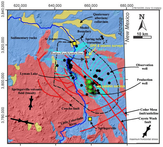
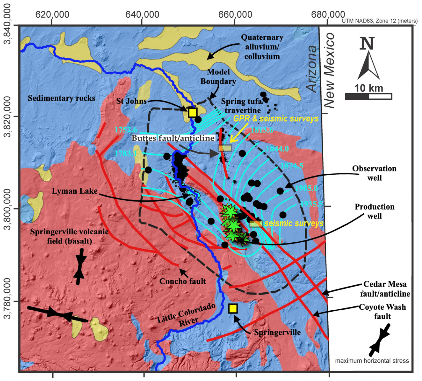
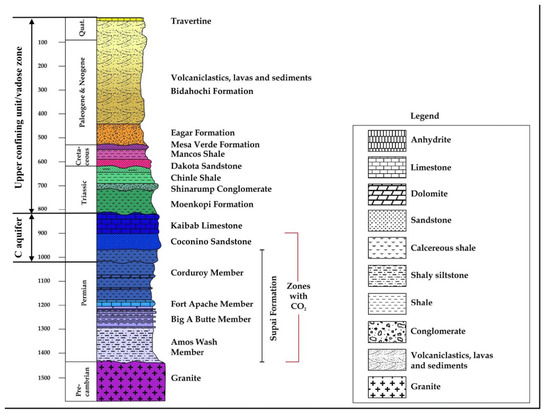
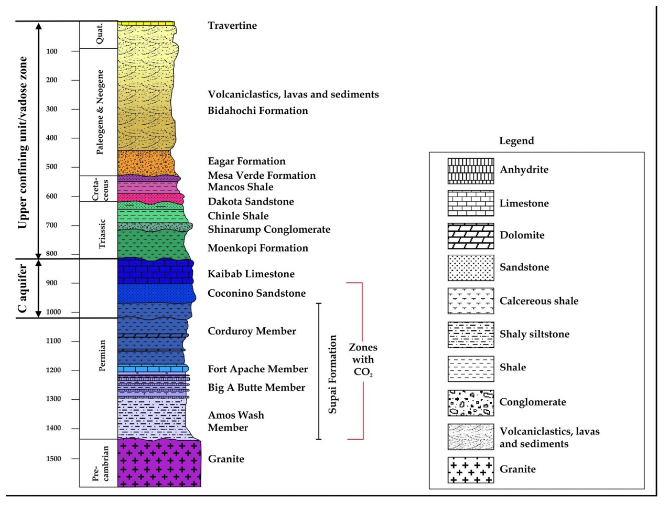
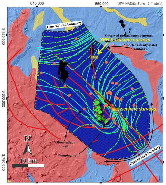
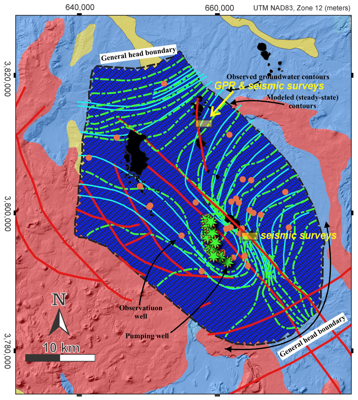
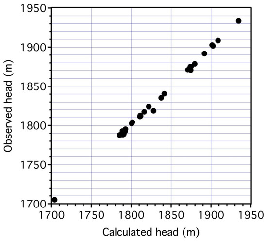
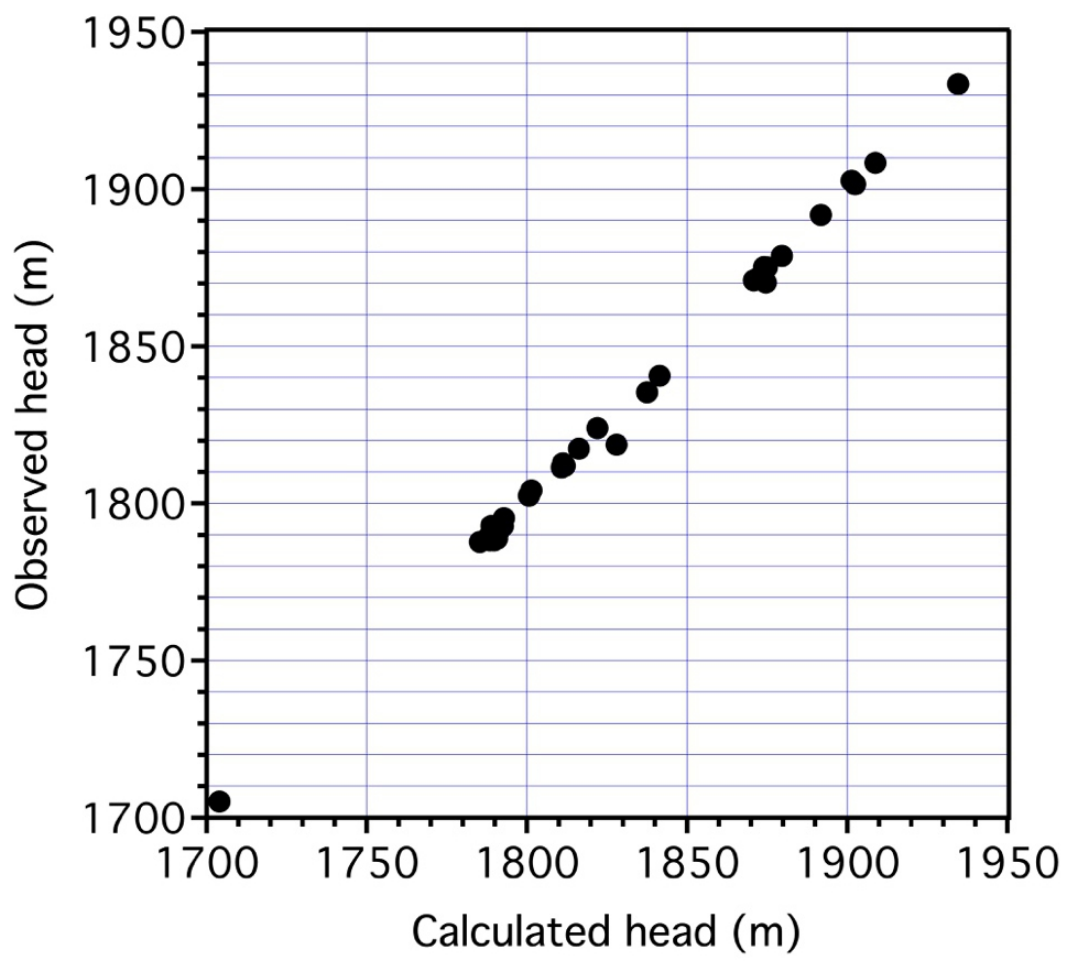
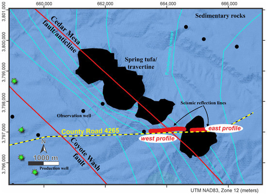
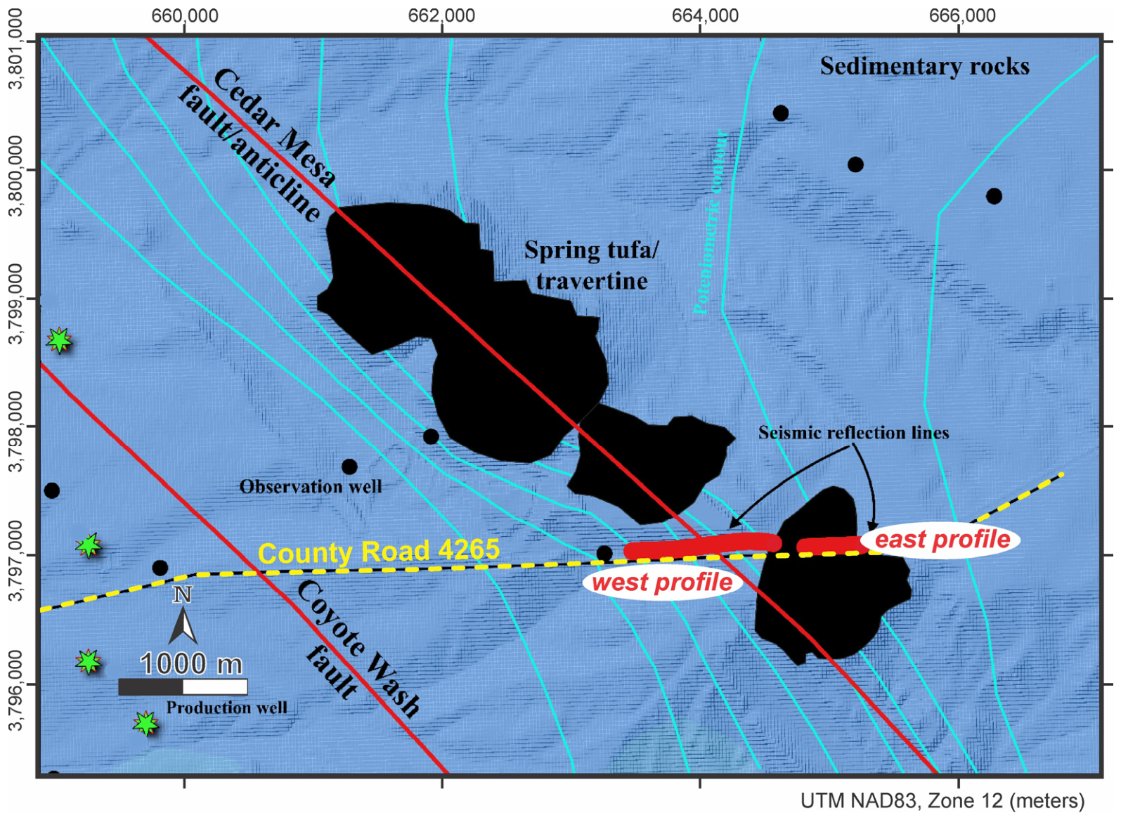
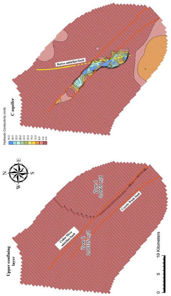
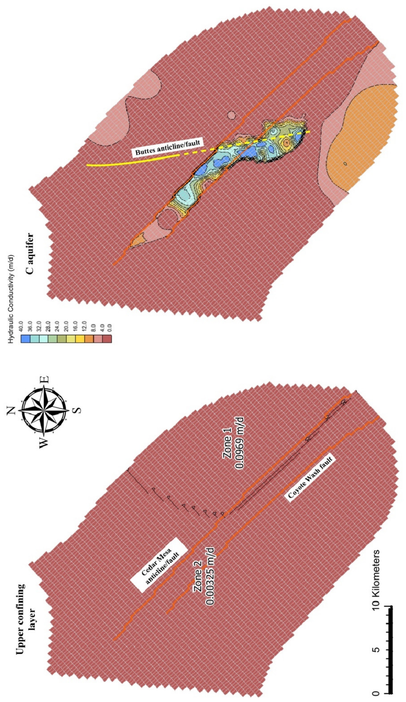
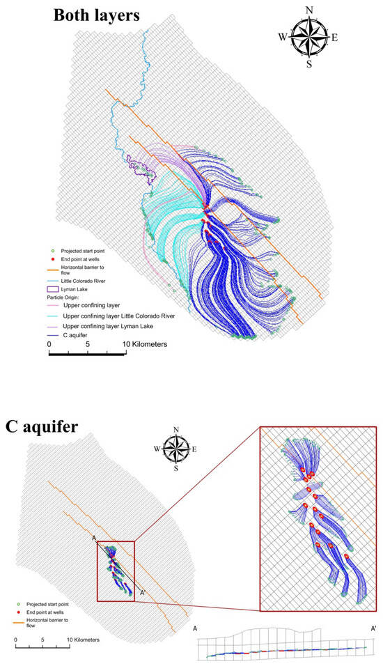
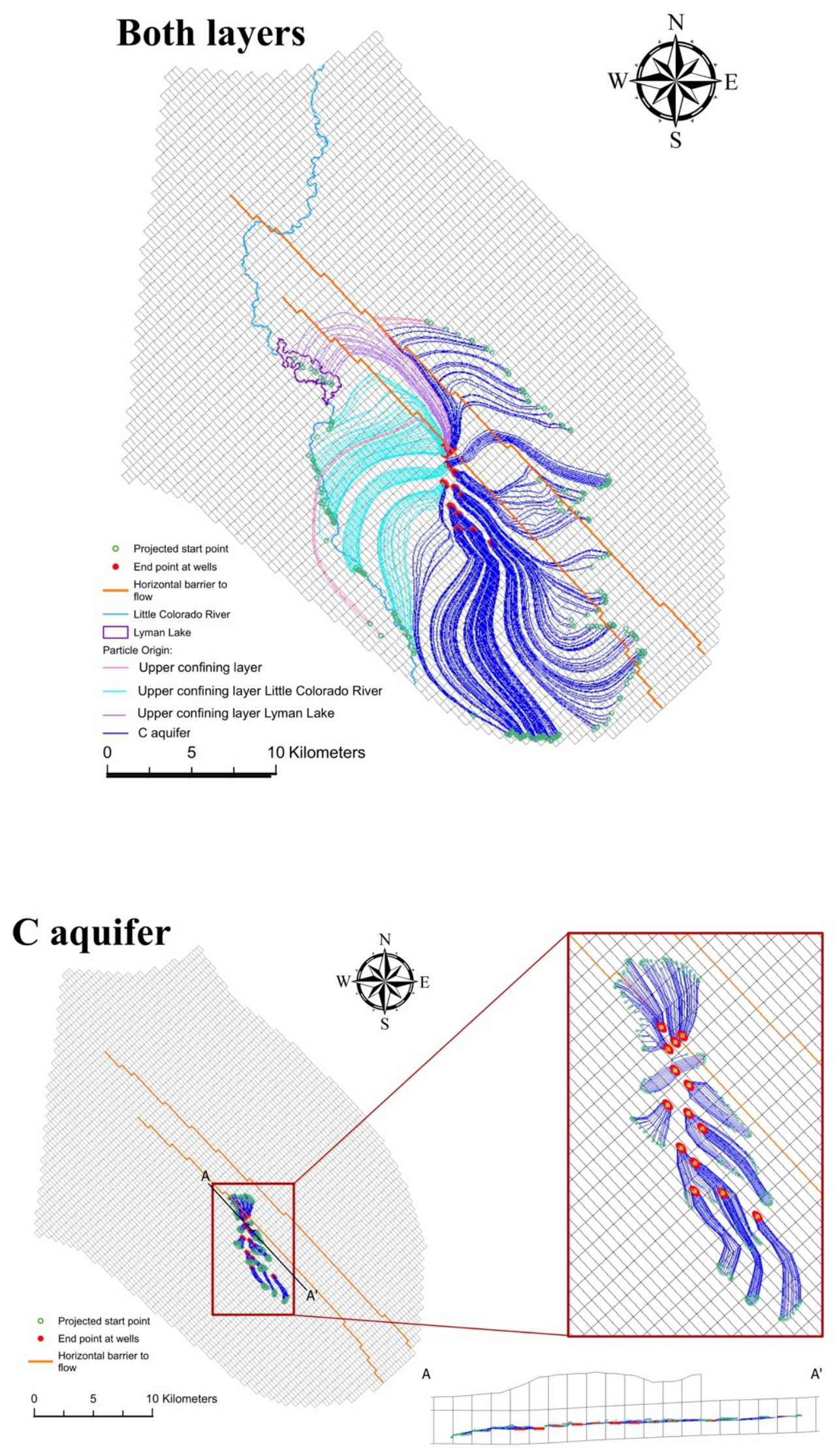
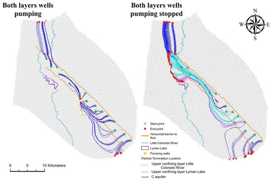
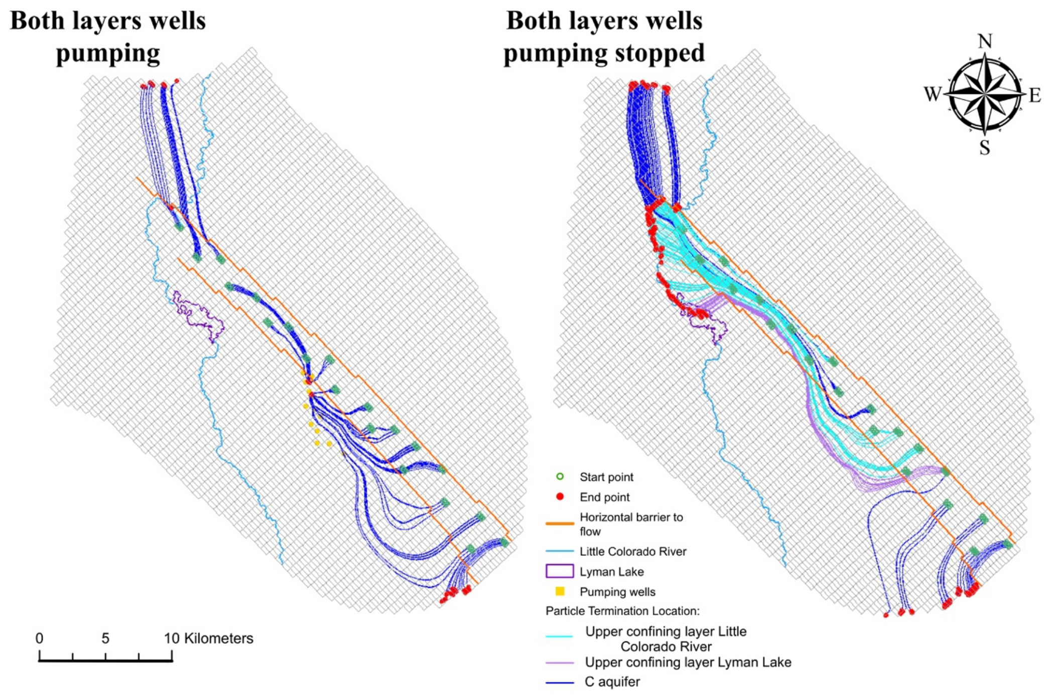
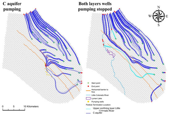
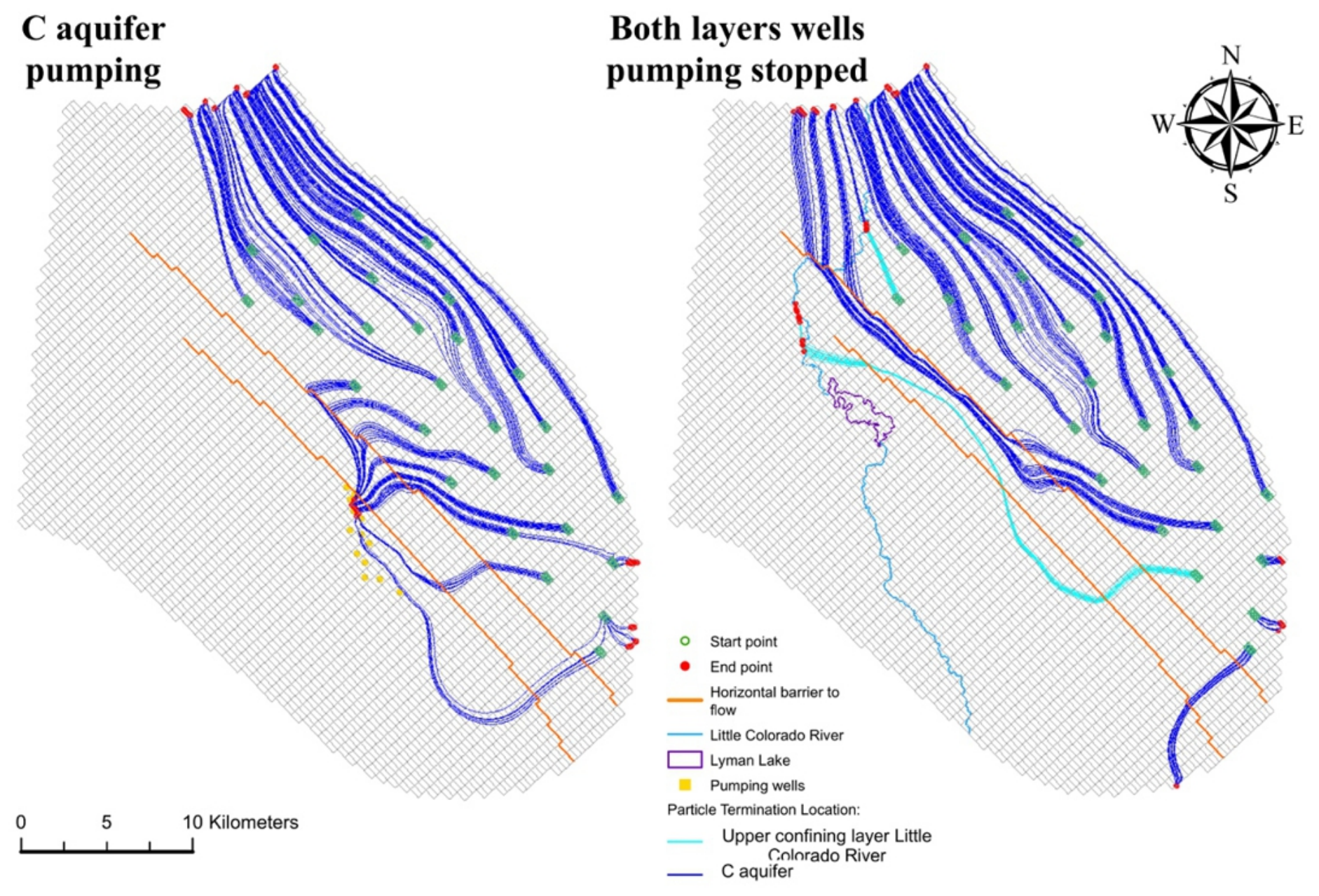
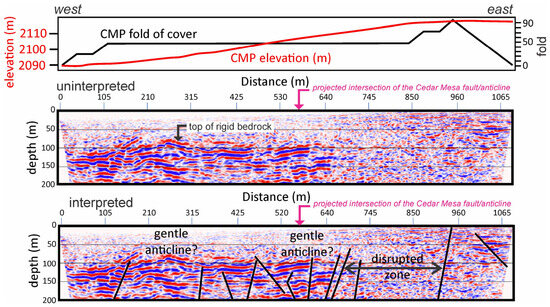
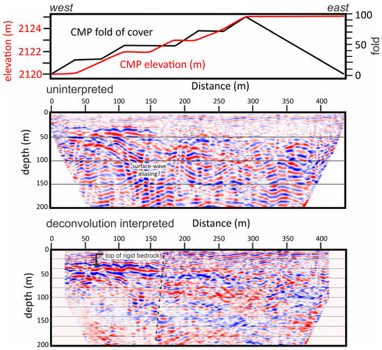
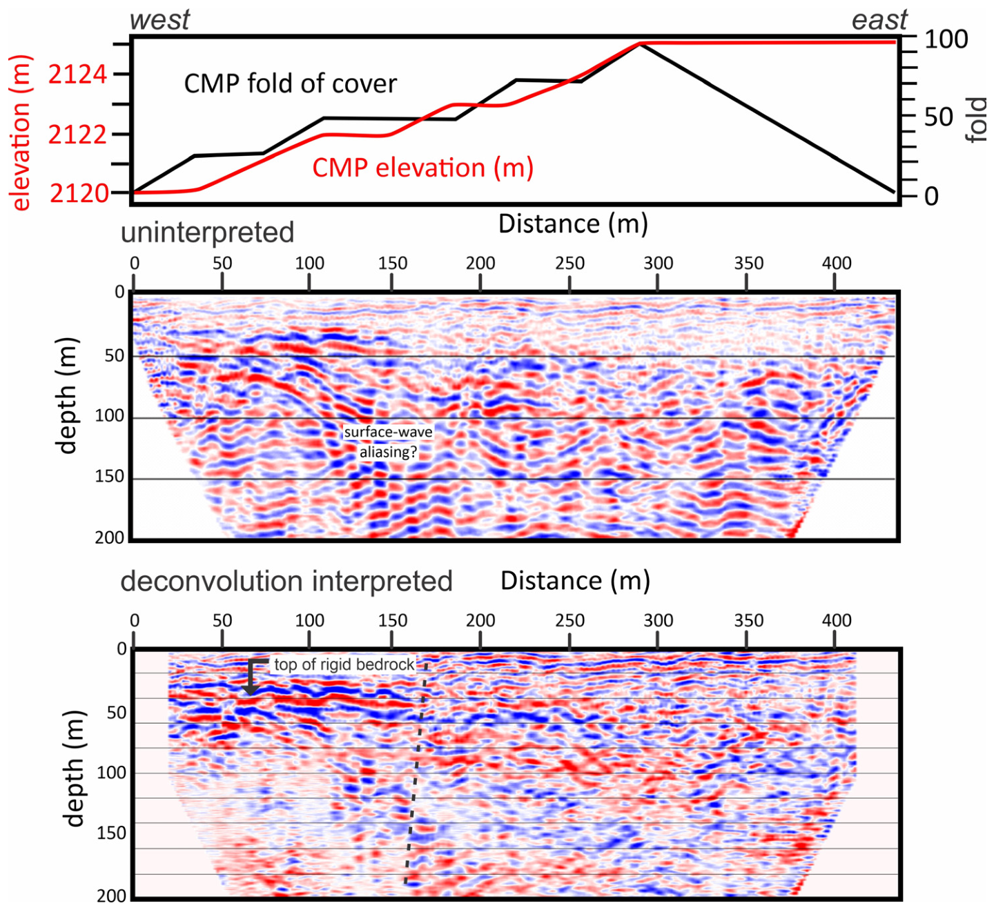
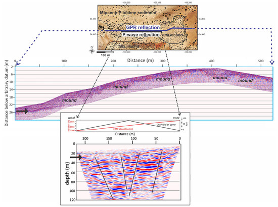
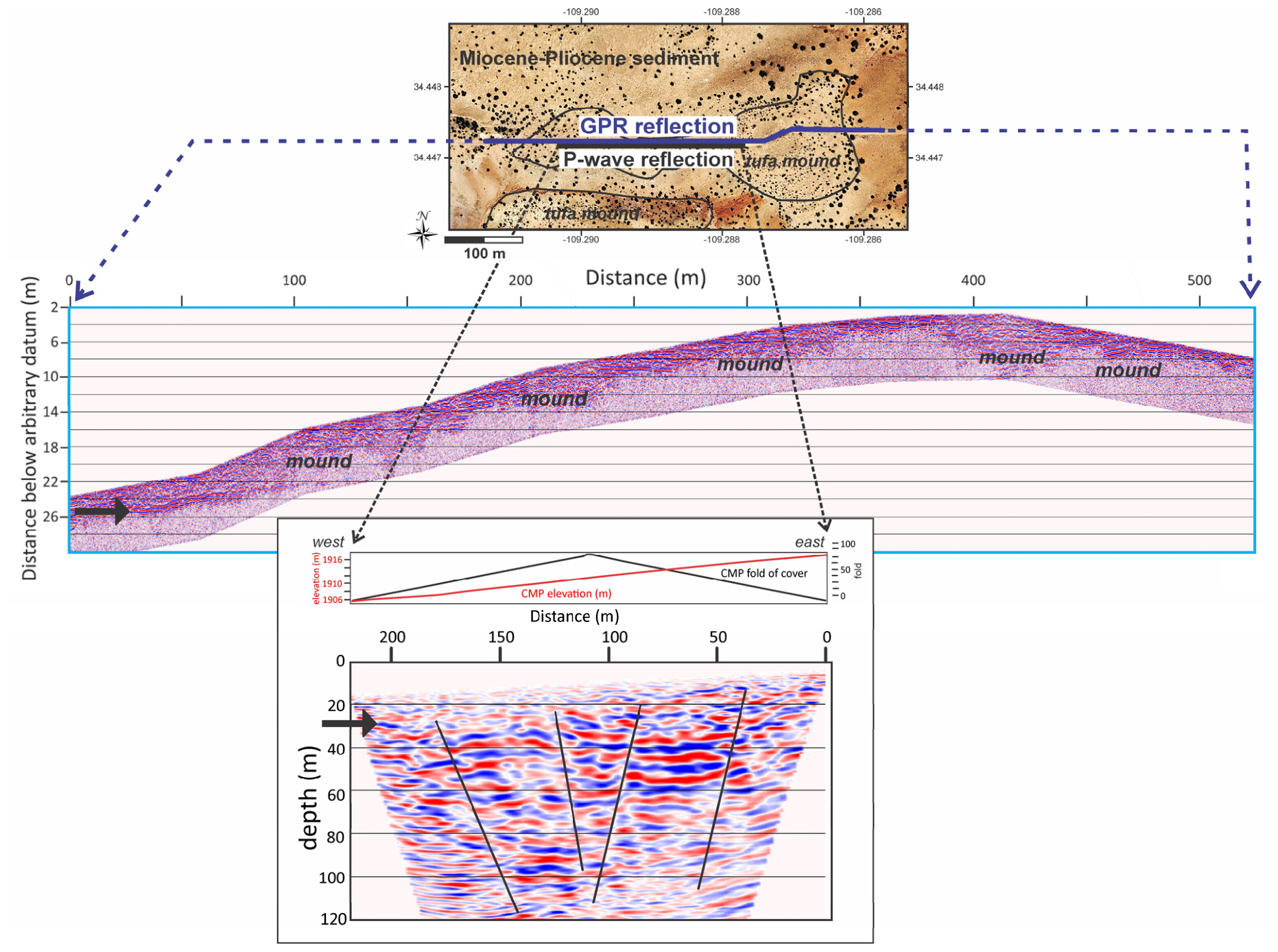

Disclaimer/Publisher’s Note: The statements, opinions and data contained in all publications are solely those of the individual author(s) and contributor(s) and not of MDPI and/or the editor(s). MDPI and/or the editor(s) disclaim responsibility for any injury to people or property resulting from any ideas, methods, instructions or products referred to in the content. |
© 2026 by the authors. Licensee MDPI, Basel, Switzerland. This article is an open access article distributed under the terms and conditions of the Creative Commons Attribution (CC BY) license.