Data-Driven Prediction Method for the Seismic Response of Cable-Stayed Bridges and Cross-Structure Calibration Motion Design

Abstract

Calibrating seismic-response surrogates for a new bridge usually requires numerous nonlinear time-history analyses (NLTHAs). This study designs a synthetic calibration motion (SCM) that supplies the calibration response through a single NLTHA. A benchmark database is established using 100 floating-system cable-stayed bridges with main spans of 210–980 m, viscous dampers and friction pendulum bearings, and 100 pairs of real bidirectional ground motions, resulting in 10,000 response histories whose input windows have horizontal peak ground accelerations (PGAs) not exceeding 0.29 g. Eleven surrogate methods are compared against the NLTHA, followed by zero- and few-motion cross-structure calibration. The proposed SCM combines a randomized-phase broadband spectrum, a non-stationary envelope and amplitude leveling. On 21 independent blind-test bridges, one universal SCM reaches approximately 81% of the matched full-supervision score obtained with 80 motions. Across all 100 bridges, one SCM comes close to ten randomly selected calibration motions and lies between the one- and three-motion results of a greedy selection that adds, one at a time, the most effective motion from the 80-motion candidate pool. Subsequent response predictions take sub-second time. By designing the calibration excitation, the method enables a new bridge’s surrogate to be calibrated with one target-bridge analysis.

1. Introduction

Cable-supported systems have continuously broken span records, with cable-stayed and suspension bridges exceeding one and two kilometers in main span, respectively [1]. As span and flexibility grow, geometric nonlinearity and the strong hysteresis of seismic isolation and damping devices become pronounced, and dynamic actions such as earthquakes and wind often govern the design. Seismic analysis must then use nonlinear time-history methods [2,3], yet one bridge under one motion typically takes minutes or even tens of minutes to compute.

Data-driven surrogate models return responses within seconds after training, but their training generally relies on dozens to a hundred nonlinear time-history samples of the same structure, and regenerating data for a new bridge almost cancels the efficiency gain. Whether a new bridge can be predicted at low computational cost, thus, decides whether such methods can be used in practice.

Data-driven structural response prediction has developed rapidly, roughly along three routes: graph neural networks that capture structural topology and member properties, sequence models that capture long-range dependencies in time-history responses, and physics-informed methods that embed mechanical priors into the model [4]. Yet the lack of benchmark datasets and the weak cross-structure generalization remain common obstacles. Deep surrogates based on graph neural networks already predict the full-process nonlinear response end to end [5] and have been extended to differentiable structural optimization, differentiable inversion, and engineering-formula discovery [6,7,8]. Their training, however, targets repeated analyses of one structure or structure family, so the training data must come from many nonlinear time-history samples of that structure itself.

On the sequence-model and lightweight-surrogate side, support vector regression and Gaussian processes serve structural reliability assessment and random vibration analysis of bridges [9,10], and surrogate–finite-element hybrids and autoregressive neural networks directly predict dynamic time histories such as wheel–rail forces [11,12]; for buildings, a convolutional–LSTM–attention network with transfer learning even reproduces nonlinear seismic responses across targets [13]. Surrogate models have also been applied to the seismic design of cable-stayed bridges: an ANN surrogate coupled with NSGA-II was used to optimize fluid viscous damper parameters [14], and a transfer-learning framework adapted a pretrained radial basis function network to a new bridge by freezing its pattern layer and recalibrating only the summation layer with about twenty additional nonlinear time-history analyses, recovering roughly 90% of the from-scratch accuracy, whereas direct transfer without adaptation shows a marked drop in accuracy [15]. On the physics-informed side, embedding physical constraints or finite-element features into the training loss improves damage identification under limited labels [16,17]. These works, however, mostly output scalar reliability indices or low-dimensional responses, or they rely on batches of finite-element samples and fine-tuning of the target structure.

As computational capability, material performance, and construction technology continue to improve, the demand for long-span cable-stayed bridges continues to grow. A technological transformation, led by new-generation materials such as carbon-fiber-reinforced polymer (CFRP) cables and ultra-high-performance concrete (UHPC), is underway, and ultra-long-span cable systems are being actively explored [18]. The theoretical span limit of steel-cable suspension bridges is about 6000 m, whereas CFRP cable systems raise it to about 10,000 m [19,20]; Meier proposed a CFRP bridge across the Strait of Gibraltar as early as 1987 [21]. Design and application methods for large-tonnage CFRP cables and the corresponding ultra-long-span systems have since been studied [22,23], and their static and dynamic performance verified [24,25]. As span and flexibility continue to increase, seismic response prediction becomes harder, making efficient methods increasingly urgent.

Existing seismic response prediction studies, however, focus on buildings such as frames and frame–shear-wall systems, and the results for flexible systems such as long-span cable-stayed bridges are still limited. Such structures are free longitudinally, have low fundamental frequencies, and are highly sensitive to structural parameters [25]; their seismic response is dominated by the strong hysteresis of devices such as viscous dampers and friction pendulum bearings, making prediction much harder than for buildings. All three routes fall short here: graph neural networks are hard to detach from the original structure, sequence models mostly output low-dimensional responses, and physics-informed methods are still largely framed around damage identification. Whether a new bridge outside the training set can obtain full-node responses at low cost has yet to be tested.

Compared with the studies above, three aspects of this work are new. First, existing surrogate models for cable-stayed bridges are trained and validated within one structure or one record set [26,27,28], so their cross-structure transferability has rarely been quantified on a common basis; the benchmark database established here provides such a basis, with 10,000 nonlinear time-history responses from 100 bridges and 100 real bidirectional motions. Second, the data cost of adapting a surrogate to a new bridge has so far been reported only for isolated cases [29,30,31], whereas here it is quantified systematically, from zero-motion transfer through to few-motion calibration. Third, and most importantly, the calibration excitation is treated as a design variable instead of being selected from a candidate set: the proposed synthetic calibration motion (SCM) inversely designs a synthetic calibration motion so that a new bridge can be calibrated with a single nonlinear time-history analysis, removing the ceiling imposed by the available records.

The objectives of this study are (i) to establish a common within-structure, new-motion benchmark for surrogate models of cable-stayed bridges; (ii) to quantify zero- and few-motion cross-structure calibration; and (iii) to develop a calibration excitation that adapts a surrogate to a new bridge using one nonlinear time-history analysis (NLTHA). The study combines a 100-bridge response database, a comparison of eleven surrogate models and the design and blind testing of a universal SCM.

Recent studies have further advanced data-driven seismic response prediction. Shao et al. [32] integrated graph attention, convolutional and recurrent networks for high-speed railway bridges; Guo et al. [33] developed a transfer-learning framework for bridge-track systems; Li et al. [26] predicted full-profile response histories using structural graph and attention features; Goswami et al. [34] applied neural operators to stochastic nonlinear structural response; Kim et al. [35] combined a simplified physics-based model with a neural operator; Chen et al. [36] introduced an attention-enhanced Fourier neural operator for stochastic seismic response and reliability analysis; Yadav et al. [37] used reservoir computing for a forced Duffing oscillator; Yan et al. [38] combined Gaussian-process surrogates with active learning for seismic fragility analysis; and Kim et al. [39] compared recorded and synthetic spectrum-compatible ground motions.

2. Database and Models

2.1. Nonlinear Finite-Element Model of the Cable-Stayed Bridge

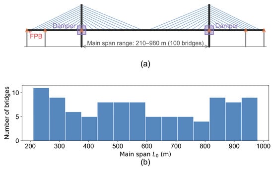
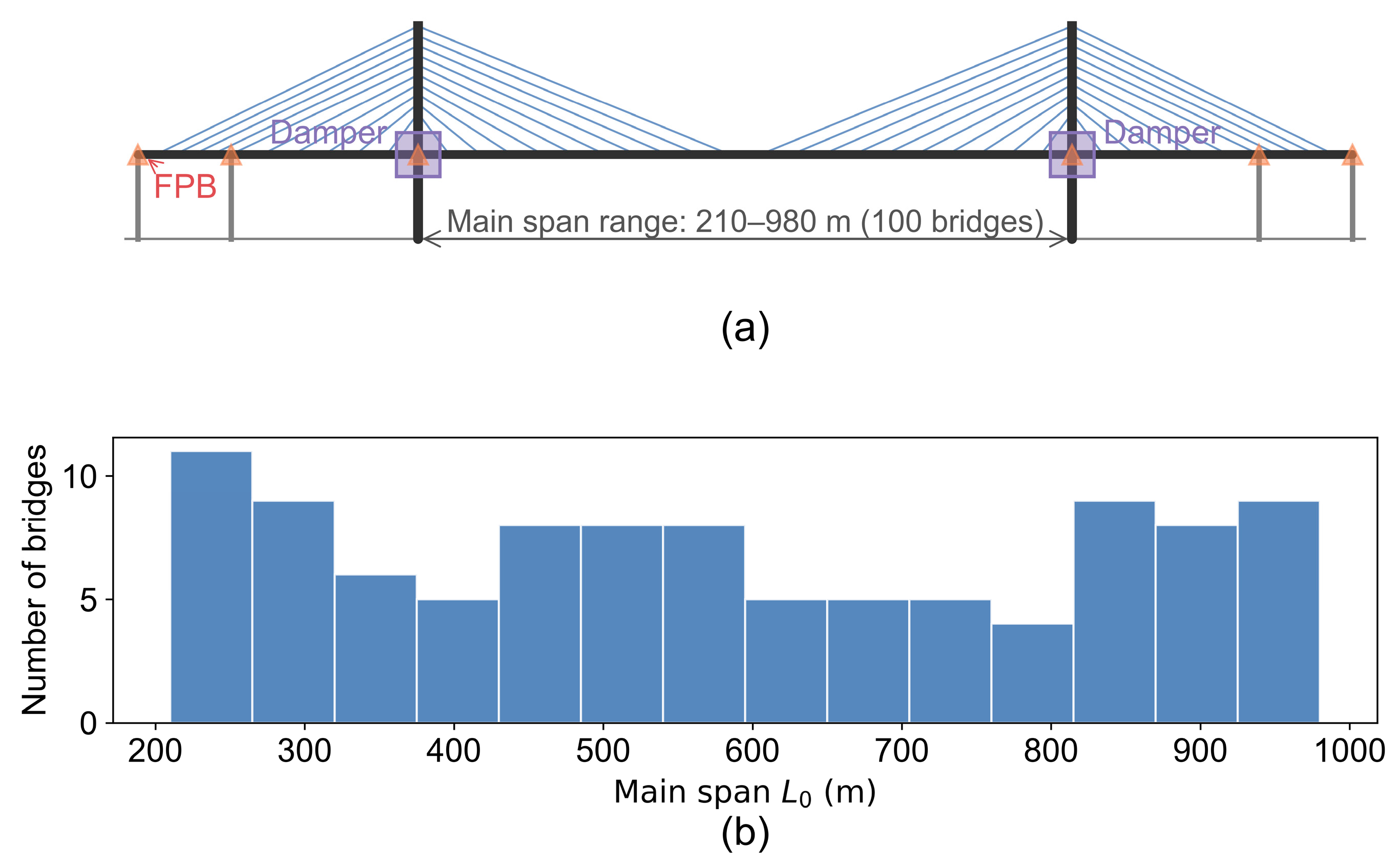
This study considers floating-system steel–concrete composite cable-stayed bridges. The girder and towers use Euler–Bernoulli beam elements, and the stay cables use truss elements, with the Ernst formula correcting the stiffness reduction from the sag effect [40]. The bridges are generated randomly from macroscopic design parameters, resulting in 100 bridges of different sizes (numbered 1–100) whose main spans uniformly cover 210–980 m, so the samples are diverse in span, stiffness, and dynamics. Table 1 lists the main design parameters and their ranges, where L₀ is the main span, H₀ the tower height above the deck, H₀/L₀ the height-to-span ratio, and L₁ the side-span length, so L₁/L₀ is the side-to-main-span ratio; the girder type and lane number are assigned randomly within their ranges.

Table 1. Main design parameters of the bridges and their ranges.

Parameter	Range
L0	210–980 m
H0/L0	0.179–0.250
L1/L0	0.345–0.485
Main girder type	twin I-girder steel composite/flat steel box girder
Structural system	floating system (seismic mitigation devices between tower and girder)
Number of lanes	3–8
Viscous damper (between girder end and tower)	velocity exponent α = 0.35; damping coefficient C = CREF·(L0/LREF)
Friction pendulum bearing (FPB) (tower–girder connection and auxiliary piers)	friction coefficient μ = 0.05; equivalent curvature radius R = RREF·(L0/LREF)

The floating system with a steel–concrete composite girder is adopted because its longitudinal flexibility and low fundamental frequencies make its seismic response sensitive to the input motion. The composite girder reduces the dead load over the span range considered. The viscous dampers and friction pendulum bearings introduce nonlinear force–velocity and force–displacement relationships, providing a representative setting for evaluating an economical surrogate-calibration procedure [41,42].

The structure contains two typical nonlinear components (Figure 1):

Figure 1. Bridge model and samples: (a) bridge model; (b) main-span distribution.

(1)

Viscous damper (between the girder end and the tower), with a continuous, preload-free constitutive relation:

$$F_d=C\dot{v}{\left({\dot{v}}^2+{\epsilon }_d^2\right)}^{{\displaystyle \frac{\alpha -1}{2}}}$$

(1)

where F_d is the damper force, v denotes the local relative displacement between the damper ends, and $\dot{v}$ is its time derivative, the relative velocity. C = C_REF·(L₀/L_REF), with C_REF = 10⁴ kN·(s/m)^α and L_REF = 240 m, is scaled linearly with the main span; α = 0.35 is the velocity exponent, and ε_d = 1 × 10⁻⁵ m/s is the numerical regularization parameter.

(2)

Friction pendulum bearing (FPB) (at the tower–girder connections and auxiliary piers), whose restoring force has a pendulum-stiffness part and a Coulomb-friction part:

$$F_f=\mathit{\mu W}\mathit{tanh}\left({\displaystyle \frac{\dot{v}}{{\epsilon }_f}}\right)+{\displaystyle \frac{W}{R}}v$$

(2)

where F_f is the bearing restoring force, v is the local relative displacement across the bearing and $\dot{v}$ is the relative velocity. The friction coefficient, μ, is given in Table 1, R = R_REF·(L₀/L_REF), RREF = 3 m, W = 0.1 times = 0.1 times the tributary deck dead load, and ε_f = 1 × 10⁻⁴ m/s. The model-generation rules scale C and R with the main span and determine W from the tributary dead load. Here, v denotes the device displacement; the response-prediction sections use v for the vertical nodal displacement.

The friction component, μW tanh($\dot{v}$/ε_f), provides a smooth transition through the velocity reversal. It is zero at a zero relative velocity and approaches ±μW for a |$\dot{v}$| much larger than ε_f. The smoothing parameter ε_f = 10⁻⁴ m/s sets the transition width and represents low-speed creep followed by saturated sliding.

The equation of motion is integrated with the implicit Newmark-β average-acceleration method (β = 0.25, γ = 0.5), using Newton–Raphson iteration to converge the nonlinear residual at each step. The integration step is 0.005 s, and the response is stored every fourth step at 0.02 s. The baseline Rayleigh calibration, D0, specifies 2% damping at the first two modes and is used consistently in the main benchmark. The first mode is the longitudinal floating mode. The frequency-dependent damping and the alternative calibration D1 are discussed in Section 4.4.3.

The planar model has longitudinal displacement, vertical displacement and in-plane rotation at each node. The girder and towers use elastic beam elements, and the cables use truss elements with Ernst equivalent moduli. The FPBs and viscous dampers supply nonlinear device forces. Modal and static comparisons with an independently assembled OpenSees model examine the structural mass, stiffness and boundary-condition implementation. Uniform horizontal and vertical support accelerations enter the inertial load, with rigid, fixed-base foundations and the constant FPB normal force, W, defined above.

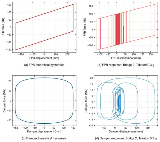
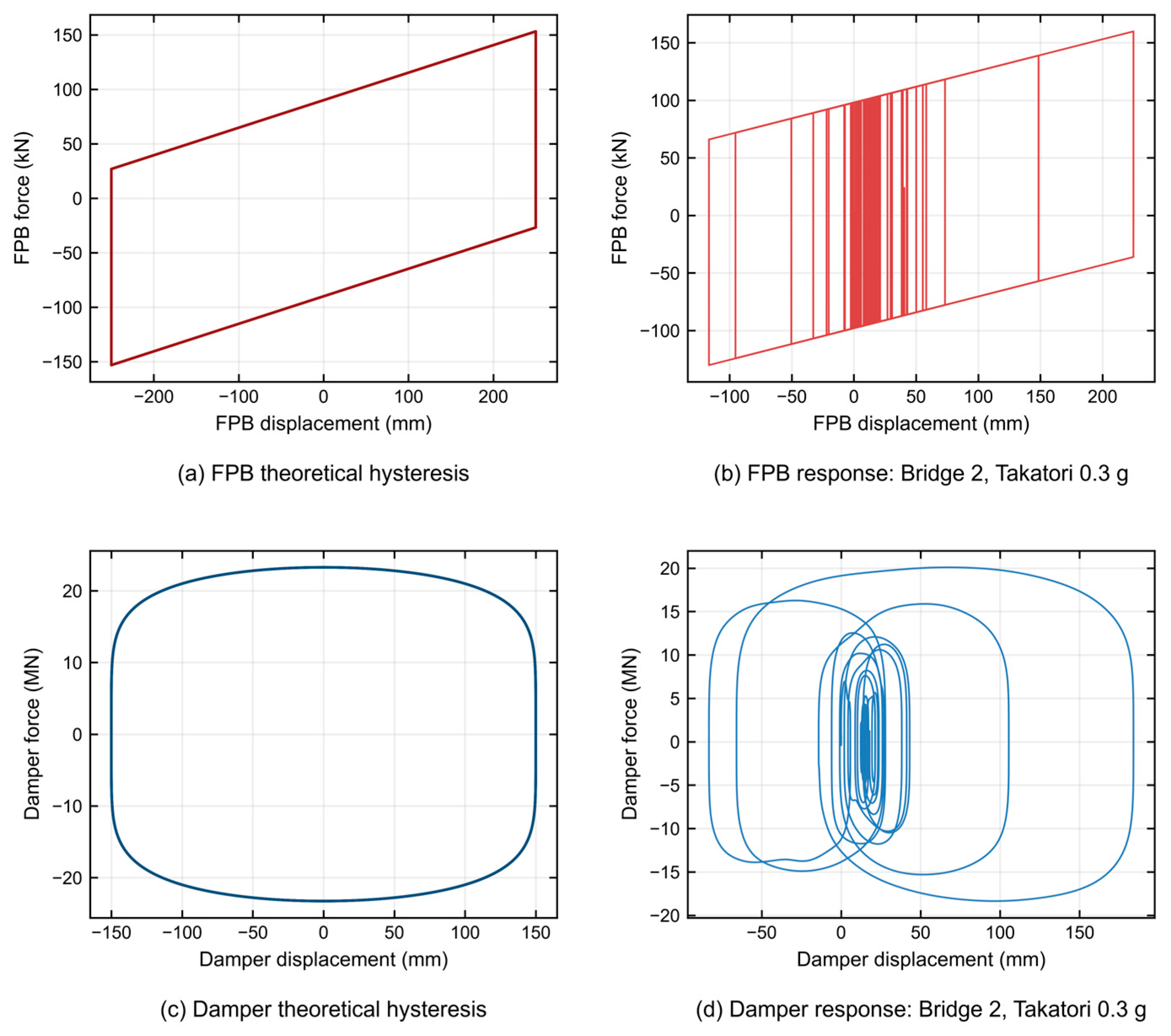
Figure 2 compares the schematic device force–displacement loops with the computed response of bridge 2 under the Takatori record at a horizontal peak ground acceleration (PGA) of 0.3 g. The FPB force combines the pendulum restoring component, Wv/R, with regularized friction, while the damper force follows its nonlinear velocity law. In this case, the selected FPB reaches a maximum absolute slip of approximately 225 mm, and the selected damper reaches a maximum absolute force of approximately 20.1 MN.

Figure 2. Device force–displacement loops: (a) schematic FPB loop; (b) computed FPB trajectory; (c) schematic viscous-damper loop; (d) computed damper trajectory.

Across the supplementary device-response cases, the selected FPB slip ranges from 4.6 to 770.8 mm and the selected damper stroke from 1.5 to 713.1 mm. The total damper dissipation ranges from 0.03 to 210.7 MJ, FPB friction dissipation from 0.02 to 3.9 MJ, and combined device dissipation from 0.06 to 214.6 MJ. The selected FPBs spend 38.8–94.7% of the analyzed record duration on the saturated-friction branch. The nonlinear-to-linear peak-displacement ratios range from 0.081 to 2.113 for the deck and from 0.200 to 3.291 for the tower.

2.2. Database of Nonlinear Seismic Responses

The input ground motions come from the NGA-West2 global strong-motion database of the Pacific Earthquake Engineering Research (PEER) Center [43]: 17 earthquakes (from the 1952 Kern County to the 2004 Niigata events), 101 stations, and 303 three-component records, covering the 1994 Northridge, 1989 Loma Prieta, 1995 Kobe, and 1992 Landers. The selection criteria are magnitude Mw 6.0–7.5, Joyner–Boore distance Rjb about 10–60 km, mostly far field, and mostly Site Class II with VS30 ≈ 260–760 m/s; all records undergo PEER standardization. Pairing the horizontal component with the largest PGA with the corresponding vertical component yields 100 ground-motion pairs as the input library for each bridge. For random ground-motion input, existing studies generate spectrum-compatible samples with non-stationary random models for random response and reliability assessment [44]; that route serves statistical quantities and reliability indices, whereas this study needs deterministic time histories of all nodes under real records.

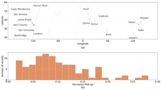
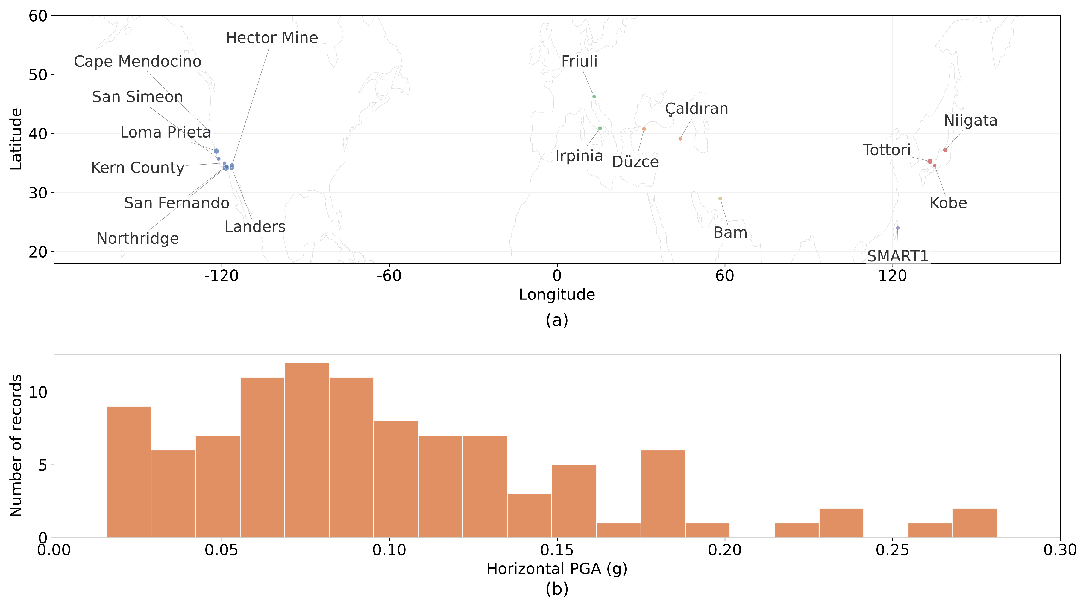
Table 2 reports horizontal PGAs of 0.0101–0.2866 g and vertical PGAs of 0.0106–0.1854 g in the analyzed input windows, with the records retaining their natural amplitudes. The input-acceleration root mean square (RMS) is 0.002–0.05 g, and the Arias intensity is 0.003–1.10 m/s. The first 20 s of each record defines the prediction window; shorter records are zero-padded. Integration uses a 0.005 s step, and stored responses contain 1000 samples at 0.02 s. The 5%-damped median horizontal response spectrum peaks at approximately 0.18 g, near T = 0.25 s. The SCM calibration uses a 60 s excitation, and Section 2.1 presents the supplementary device-response cases.

Table 2. Key parameters of the input ground motions (100 pairs).

Parameter	Range	Mean
Horizontal PGA	0.01~0.29 g	0.10 g
Vertical PGA	0.01~0.19 g	0.06 g
Input RMS	0.002~0.05 g	0.02 g
Arias intensity	0.003~1.10 m/s	0.21 m/s
Original record duration	10.4~300 s	85.6 s

Each bridge is subjected to the 100 bidirectional ground-motion pairs for nonlinear time-history analysis, yielding 100 × 100 = 10,000 nonlinear time-history samples; each contains the longitudinal displacement, u, and vertical displacement, v, of all nodes within 20 s, together with the input acceleration. The epicenters and PGA distribution are shown in Figure 3, where the marker size indicates the number of stations.

Figure 3. Input ground-motion information: (a) epicenter distribution; (b) horizontal PGA distribution.

The 100 motions of each bridge are divided by a fixed random partition into 80 training, 10 validation, and 10 test motions, and all experiments use the same partition for comparability. The test motions take no part in training or selection.

Three considerations set the size of the record set. (i) Coverage: the horizontal PGA spans 0.0101–0.2866 g and the vertical 0.0106–0.1854 g, two orders of magnitude, and the spectral content ranges from narrowband pulse-like to broadband, so the set brackets the excitation conditions of practical interest while remaining affordable for 100 bridges. (ii) Statistical stability: with the fixed 80/10/10 partition, each bridge retains ten test motions, which is sufficient for stable per-bridge statistics and, across 100 bridges, for stable aggregate comparisons. (iii) Scale closure: 100 bridges × 100 motions yields the 10,000 nonlinear time-history responses that underlie every benchmark and calibration experiment reported below.

3. Surrogate Models and Benchmark for Within-Structure Seismic Response

3.1. Prediction Task and Evaluation Metrics

Given a bridge’s bidirectional ground-acceleration history, a(t) = [a_x(t), a_y(t)], with 1000 samples at 0.02 s, the surrogate predicts longitudinal and vertical nodal displacement histories, u(t) and v(t). The overall scores are evaluated on the deck and tower response nodes, with n denoting the node count for the corresponding direction. Matched SCM and full-supervision comparisons use the same response nodes and test motions.

The 100 motions of each bridge are divided by a fixed random seed into 80 training/10 validation/10 test motions, yielding 8000 training, 1000 validation, and 1000 test motions across all bridges. Data-driven methods are fitted only on the training motions; the validation motions monitor development; all reported numbers come from the test motion, which takes no part in fitting or selection. The FEM has no training/validation split, and its output is the ground truth.

For each motion sample and each direction, the error is computed independently as the root mean square over time × nodes:

(1)

Primary metric, Zero-baseline normalized root-mean-square error (NRMSE): Zero-baseline NRMSE = 1 − RMSE($\hat{y}$, y)/RMS(y), which uses the RMS of the true response as the denominator; 1 denotes a perfect prediction and 0 a constantly-zero prediction. This metric is stricter and more discriminative and suits strictness checks and ablation analysis.

(2)

Secondary metric, Peak-normalized NRMSE: Peak-normalized NRMSE = 1 − RMSE($\hat{y}$, y)/max|y|, where RMSE is the root-mean-square prediction error and max|y| the absolute peak of that sample’s response; the closer to 1 the better. This metric measures the normalized overall error, not the pointwise peak error; the peak error Epeak = |max|$\hat{y}$| − max|y||/max|y| is reported separately.

The u and v directions are reported separately, with the overall value being their mean. Unless stated otherwise, tables report single-factor sweeps on the development bridges or within-structure benchmarks.

3.2. Candidate Methods

This section establishes a common benchmark for within-structure, new-motion prediction. The surrogate models are trained on 80 motions of one bridge and evaluated on held-out motions of that bridge. Eleven surrogate methods are compared with nonlinear time-history analysis (NLTHA), which supplies the ground-truth responses. Table 3 summarizes the candidate methods.

Table 3. Candidate methods for the within-structure, new-motion task.

Category	Method	Training Requirement
Ground truth	NLTHA (nonlinear time-history analysis)	none (the truth itself)
Physics-based	mode superposition method (MSM), H1 frequency-domain method	0/1-motion calibration
Data-driven	FIR, VARX(8/16/32), PCA-ARX, ESN	80 motions
Hybrid	V2 (32VARX + PCA), V3 (FIR + 32VARX + PCA), VR-ESN (32VARX + residual ESN)	80 motions

All methods use the same 80/10/10 training, validation and test partition. The model trained on 80 target-bridge motions provides the full-supervision reference for the calibration comparisons.

All methods share the following definitions:

Data-driven methods first represent the response in a low-dimensional spatial basis. A linear eigenvalue analysis Kφ = ω² Mφ is performed once for each bridge, where K and M are the stiffness and mass matrices and ω and φ are the circular frequency and mode shape. The lowest six eligible mode shapes with f ≥ 0.01 Hz are evaluated at the response nodes. After spatial-mean removal, columnwise RMS normalization and QR orthogonalization, a uniform translation vector 1/√n is prepended to form the orthonormal basis Φ ∈ R^n_X7:

$$\Phi =\left[{\displaystyle \frac{1}{\sqrt{n}}},\mathit{orth}\left({\phi }_1-{\bar{\phi }}_1\right),\dots ,{\phi }_6-{\bar{\phi }}_6\right]$$

(3)

In Equation (3), n is the number of response nodes, φ_i is the spatial vector of the i-th retained mode on those nodes, and orth(·) denotes columnwise orthogonalization. The generalized coordinates q(t) = Φ^Ty(t) yield seven channels per direction, and the response is reconstructed as $\tilde{y}$(t) = Φ$\hat{q}$(t).

All data-driven methods are fitted independently by direction and by bridge, using the generalized-coordinate sequences of the 80 training motions. Linear regression uses scaled ridge: coefficients C = (G + λI)⁻¹ X^T Y, with λ = α·tr(G)/P, G = X^T X, P the number of features, X and Y the design and target matrices, and I the identity matrix; α is a dimensionless regularization coefficient, and the design-matrix columns are RMS-normalized.

At test time, only the input acceleration is given; the model advances autoregressively for 1000 steps from zero initial conditions and then reconstructs the nodal displacements.

The 12 methods, including the baselines, are as follows:

(1)

Nonlinear time-history analysis (NLTHA): Ground-truth baseline, the implicit Newmark-β integration of the bridge’s nonlinear finite-element model in Section 2 (member constitutive laws, bearings, and structural damping as in Equations (1) and (2) and Rayleigh damping). Its output on the test motions is the ground truth, so it needs no training and both metrics equal 1 by definition. Its computation time is the wall-clock time recorded per motion during database generation (single-core, single-BLAS thread).

(2)

Mode superposition method (MSM): A linear physical approximation that takes the first 30 modes (f ≥ 0.01 Hz) of the same bridge, decouples each mode into a single-degree-of-freedom system, integrates each with the Newmark method, and superimposes the results; zero training. The MSM is an elastic model that ignores the FPB and dampers.

The MSM retains the lowest 30 eligible modes with f ≥ 0.01 Hz. The same truncation rule is applied to all 100 bridges.

$${\ddot{q}}_m+2{\zeta }_m{\omega }_m{\dot{q}}_m+{\omega }_m^2{q}_m=-g_{m}a\left(t\right),g_m={\displaystyle \frac{{\phi }_m^T\mathit{Mr}}{{\phi }_m^{T}M{\phi }_m}},y\left(t\right)=\sum _m{\phi }_m{q}_m\left(t\right)$$

(4)

In Equation (4), q_m, ζ_m, and ω_m are the modal coordinates, modal damping ratio, and circular frequency of the m-th mode; gm is the modal participation factor; φ_m is the m-th mode shape; M is the mass matrix; r is the direction-indicator vector; and y(t) is the nodal displacement response.

(3)

H1 frequency-domain transfer function (H1): The first training motion of the bridge estimates the per-node frequency-domain transfer function (Equation (5)); at prediction, $\hat{U}$(ω) = H(ω)·A(ω) is applied to the target motion and inverse-FFT back to the time history. Only one motion is calibrated, with no free-parameter fitting.

$$H\left(\omega \right)=U\left(\omega \right)·{\displaystyle \frac{\mathit{conj}\left(A\left(\omega \right)\right)}{{\left|A\left(\omega \right)\right|}^2+\epsilon {\left|A\right|}_{\stackrel{2}{\mathit{max}}}}},\epsilon ={10}^{-6}$$

(5)

In Equation (5), U(ω) and A(ω) are the spectra of the output displacement and input acceleration, conj(·) is the complex conjugate, and ε is a regularization term. At prediction, $\hat{U}$(ω) = H(ω)·A(ω), and the inverse FFT yields the time history; u and v are treated independently.

(4)

Finite impulse response filter (FIR): a two-channel causal FIR filter fitted on the generalized coordinates (Equation (6); 128 orders, 256 lag features), columnwise RMS-normalized and solved with scaled ridge (α = 1.0).

$$q_t=\sum _{l=0}^{127}{C}_l{a}_{t-l},C_l\in R^{2\times 7}$$

(6)

In Equation (6), q_t is the generalized coordinate, at denotes the input acceleration, and C_l the l-th-order coefficient matrix.

(5)

8th-order vector autoregression with exogenous inputs (8VARX): a linear dynamic model on the generalized coordinates (Equation (7)), where Al and Bl are the autoregressive and exogenous-input coefficient matrices, and p and r are the autoregressive order and the number of exogenous lags. Here p = 8 and r = 16, with scaled ridge α = 1 × 10⁻⁶ and a spectral-radius stability projection after fitting.

$$q_t={\displaystyle \sum _{l=1}^p}{A}_l{q}_{t-l}+{\displaystyle \sum _{l=0}^{r-1}}{B}_l{a}_{t-l}$$

(7)

(6)

16th-order VARX (16VARX): same as 8VARX but with p = 16, r = 32, and α = 1 × 10⁻⁸.

(7)

32nd-order VARX (32VARX): same as 8VARX but with p = 32, r = 64, and α = 1 × 10⁻⁸.

(8)

Principal component analysis–autoregressive (PCA-ARX): unlike the physical modal basis, its spatial basis comes entirely from the training data; a truncated SVD of the training responses takes the first seven principal components as the basis, and each channel fits a diagonal VARX (p = 32, r = 32, α = 1 × 10⁻⁸) before reconstruction.

(9)

Echo state network (ESN): A fixed random reservoir plus a linear readout, with only the readout trained; the reservoir updates as in Equation (8) (512 states, spectral radius ρ = 0.98, and leak rate λ = 0.2). Because its spatial basis is obtained by PCA of the response and only the linear readout is fitted, this implementation is referred to as PCA-ESN.

$$s_t=(1-\lambda )s_{t-1}+\lambda ·\tanh (\rho ·\sigma \odot \mathit{roll}(s_{t-1},1)+\gamma ·W_{\mathit{in}}·{\tilde{a}}_t)$$

(8)

Here, s_t is the reservoir state vector, λ the leak rate, ρ the reservoir spectral radius, W_in the input matrix, γ the input scaling coefficient, σ ∈ {±1} the sign vector, roll(·,1) the circular shift, and $\tilde{a}$_t the RMS-normalized acceleration. The readout maps [s_t, $\tilde{a}$_t] to the first 12 SVD principal-component coordinates of the training response; the first 32 steps are treated as washout and do not participate in the fitting, and the response is then reconstructed through this SVD basis into nodal displacements.

(10)

V2 (bounded blend): A linear mixture of 32VARX and PCA-ARX, and $\hat{y}$ = w₁·32VARX + w₂·PCA-ARX. The weights are fitted per direction and per bridge on the training motions by minimizing the sum of squared errors between the blend and the truth (ridge α = 1.0 and weights bounded between 0.05 and 2.0) to prevent collapse onto a single submodel.

(11)

V3 (bounded blend): a linear mixture of FIR, 32VARX, and PCA-ARX, $\hat{y}$ = w₁·FIR + w₂·32VARX + w₃·PCA-ARX, and fitted as V2.

(12)

VARX-residual echo state network (VR-ESN): 32VARX first yields a baseline prediction dominated by the physical structure, then an ESN learns the residual r = y − $\hat{y}$32VARX; the residual readout uses peak-weighted ridge regression (equal weight in u and peak weight β = 10 in v) to focus on peak periods of large responses.

$$\hat{y}={\hat{y}}_{32\mathit{VARX}}+\mathit{ESN}(r;a)$$

(9)

In Equation (9), $\hat{y}$_32VARX is the baseline prediction of 32VARX and ESN(r; a) the ESN correction for the residual, r. The residual ESN uses the same reservoir structure, but its readout targets the first 12 SVD principal components of the residual with peak-weighted ridge regression: the time-step weight, w_t = 1 + β·‖r_t‖_nodes, the spatial RMS of the residual at that step, focuses the fitting on peak periods. β is 0 for u and 10 for v.

The node-wise spatial RMS of the residual at time step t, used as the weight of the residual readout, is defined by Equation (10), where r_t,i is the residual at node i of the retained nodal set (n nodes), and the summation runs over the nodes; the sample weight of the peak-weighted ridge regression follows as w_t = 1 + beta·||r_t||_nodes, with beta = 0 for the longitudinal direction u and beta = 10 for the vertical direction, v.

$${\Vert r_t\Vert }_{\mathit{nodes}}=\sqrt{{\displaystyle \frac{1}{n}}{\displaystyle \sum _{i=1}^n}{r}_{t, i}^2}$$

(10)

3.3. Comparison Results and Benchmark

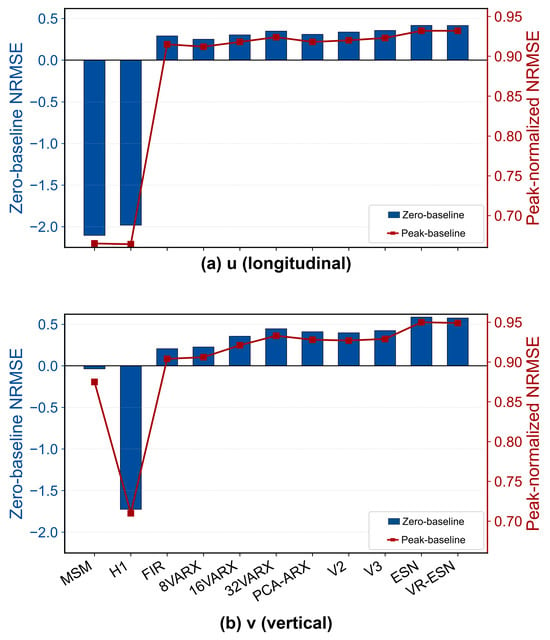
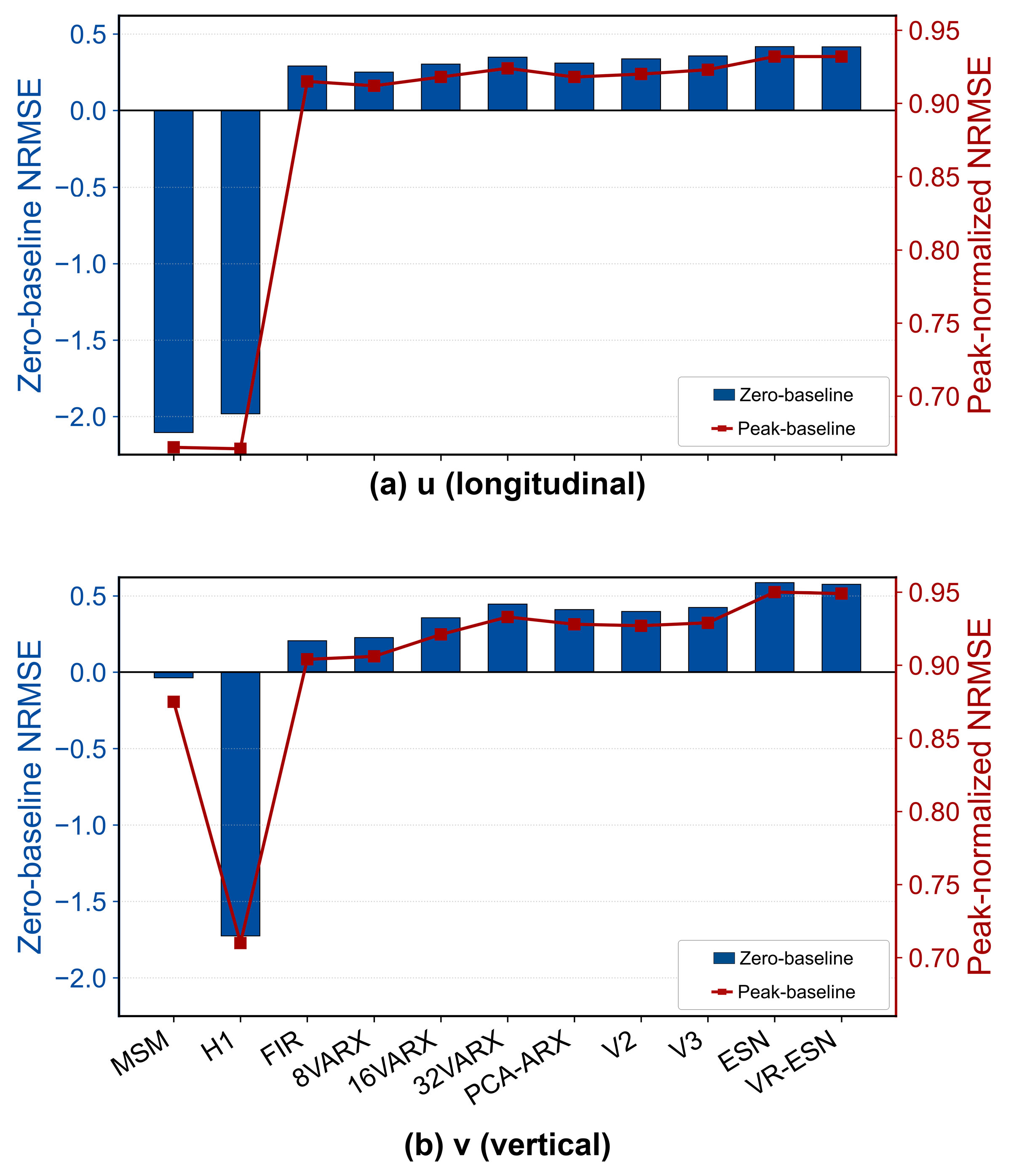
Table 4 and Figure 4 yield the overall accuracy of the candidate methods, with Zero-baseline NRMSE as the primary metric and Peak-normalized NRMSE the secondary. Table 5 presents the single-core computation time on a typical desktop personal computer for the full 20 s analysis, grouped into small (200–450 m), medium (450–750 m), and large (750–1000 m) spans.

Table 4. Comparison on the within-structure, new-motion task.

Method	Peak-Normalized NRMSE u	Peak-Normalized NRMSE v	Peak-Normalized NRMSE Overall	Zero-Baseline NRMSE u	Zero-Baseline NRMSE v	Zero-Baseline NRMSE Overall	Epeak u	Epeak v
NLTHA (truth)	1.000	1.000	1.000	1.000	1.000	1.000	0.000	0.000
ESN	+0.932	+0.950	+0.941	+0.417	+0.586	+0.502	0.151	0.180
VR-ESN	+0.932	+0.949	+0.940	+0.415	+0.575	+0.495	0.151	0.182
32VARX	+0.924	+0.933	+0.928	+0.348	+0.446	+0.397	0.309	0.357
V3	+0.923	+0.929	+0.926	+0.356	+0.423	+0.389	0.415	0.411
PCA-ARX	+0.918	+0.928	+0.923	+0.310	+0.410	+0.360	0.208	0.354
V2	+0.920	+0.927	+0.923	+0.337	+0.397	+0.367	0.486	0.478
16VARX	+0.918	+0.921	+0.920	+0.303	+0.356	+0.330	0.283	0.396
FIR	+0.915	+0.904	+0.910	+0.290	+0.206	+0.248	0.462	0.545
8VARX	+0.912	+0.906	+0.909	+0.251	+0.227	+0.239	0.346	0.564
MSM	+0.665	+0.875	+0.770	−2.105	−0.036	−1.071	0.560	0.599
H1	+0.664	+0.710	+0.687	−1.982	−1.726	−1.854	0.810	0.611

Note: Epeak is the median over the 10 test motions (smaller is better). All hyperparameters are set only on the training/validation sets; the test motions are used once, in the final evaluation.

Figure 4. Comparison of the 11 surrogate methods: (a) Zero-baseline NRMSE; (b) Peak-normalized NRMSE.

Table 5. Computation time.

Method	Training (Fitting) per Bridge (s)	Small Bridge (s)	Medium Bridge (s)	Large Bridge (s)
NLTHA (truth)	—	31.5	50.4	214.8
MSM	0	0.101	0.110	0.110
H1	≈0 (one-motion calibration)	0.002	0.003	0.003
FIR	2.7	0.006	0.007	0.006
8VARX	1.4	0.022	0.022	0.022
16VARX	2.7	0.042	0.038	0.039
32VARX	5.8	0.083	0.071	0.076
PCA-ARX	18.2	0.085	0.076	0.083
V2	38.3	0.180	0.152	0.162
V3	41.0	0.186	0.159	0.168
ESN	17.2	0.049	0.049	0.055
VR-ESN	17.9	0.136	0.128	0.122

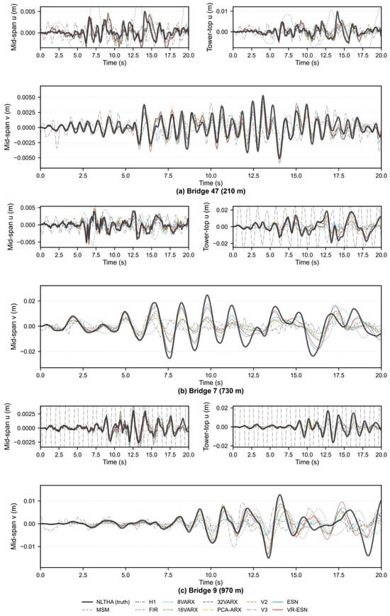
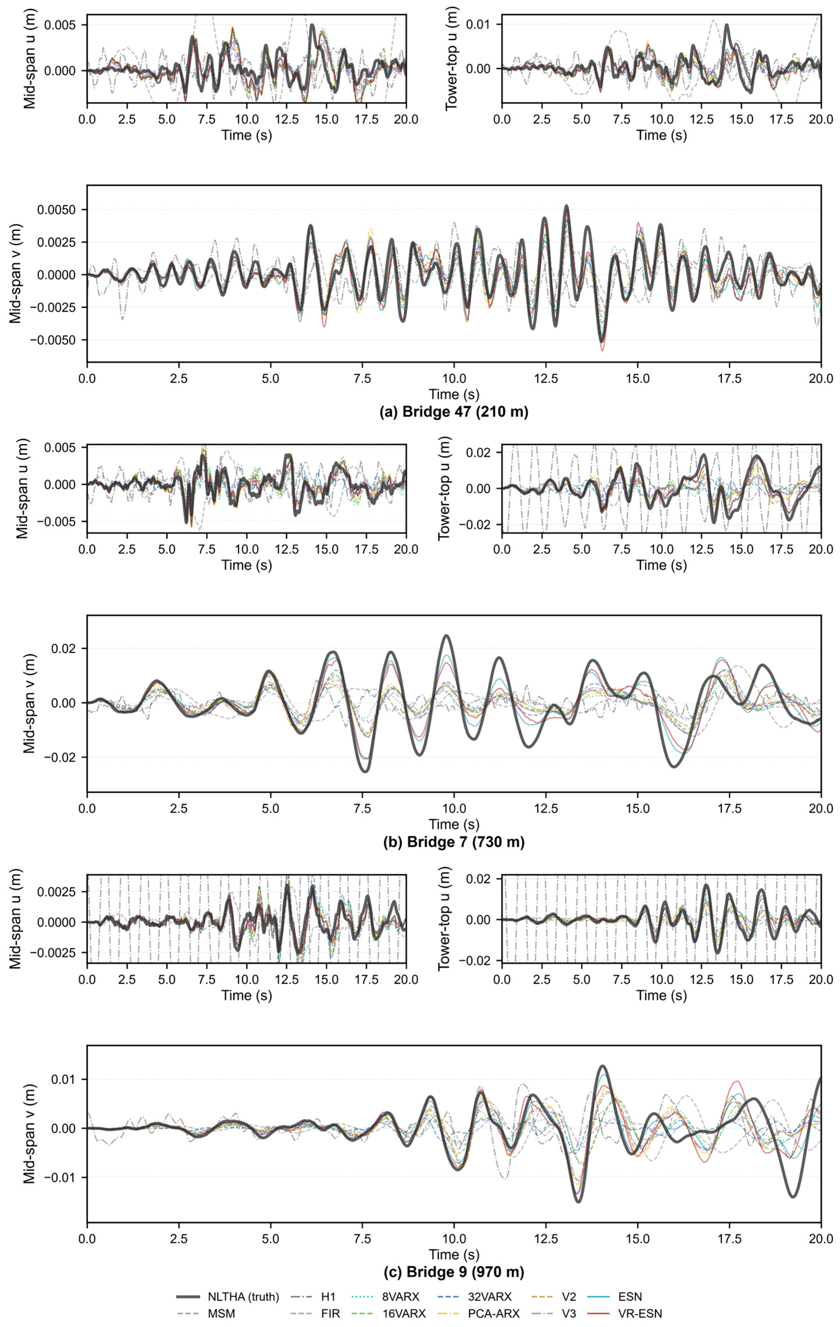
To examine the time-history predictions, Figure 5 compares the displacement responses of three bridges under their test motions: Bridge 47 (small, 210 m), Bridge 7 (medium, 730 m), and Bridge 9 (large, 970 m) in panels (a–c). For each bridge, the upper row shows the mid-span and tower-top longitudinal (u) responses, and the lower panel shows the mid-span vertical (v) response with a doubled plotting width and height for readability. The dark-gray curves are the ground truth, and the rest are the 11 surrogate predictions. Panels (a–c) correspond to Bridges 47, 7 and 9. The vertical limits follow the ground-truth extrema with 15% padding.

Figure 5. Typical time-history predictions.

From the above analysis, the main findings are as follows:

ESN and VR-ESN produce the highest overall scores among the eleven surrogate methods, with similar scores (Table 4). The H1 and mode-superposition baselines have negative overall Zero-baseline scores. Across the 100 bridges and ten test motions, the coefficient of determination of the peak displacement is R² ≈ 0.87.

The modal-basis dimension is the single largest gain. As it increases, the Zero-baseline NRMSE rises from +0.26 to +0.39, with the vertical gain especially clear, and saturates after principal-component dimension 7. The VARX order yields a monotonic but diminishing gain.

The surrogate methods have a large speed advantage. The best method predicts one motion in 0.05–0.14 s, nearly independent of span; the FEM computation takes from about 31.5 s to 215 s as the span grows, so the VR-ESN speedup is about 230–1800× and the ESN about 640–3900×. The FEM is, thus, only suited to generating the database, not to repeated prediction.

The key to accuracy lies in the data. The best method reaches a Peak-normalized NRMSE of +0.94 under 80 training motions, but this depends entirely on within-structure data, and the inter-bridge differences of the readout carry all of the performance. The question then turns to new bridges: how to obtain equal accuracy at minimum data cost for a bridge outside the training set.

4. Cross-Structure Generalization and New-Bridge Calibration

This chapter studies bridges outside the training set, asking what nonlinear response prediction can be obtained with few, or even zero, motions. It proceeds in four steps: the difficulty of direct transfer, the performance curve of few-motion calibration, the value of motion selection, and, finally, the SCM designed from the characteristics of good motions.

4.1. Difficulty of Direct Transfer Under the Strategies Examined

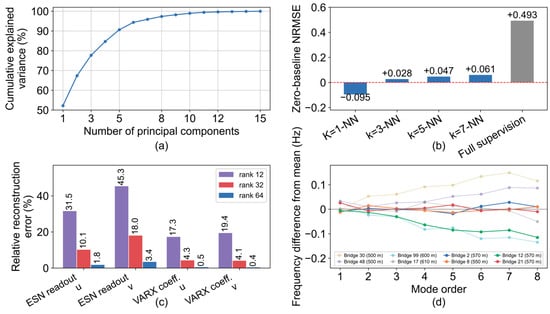
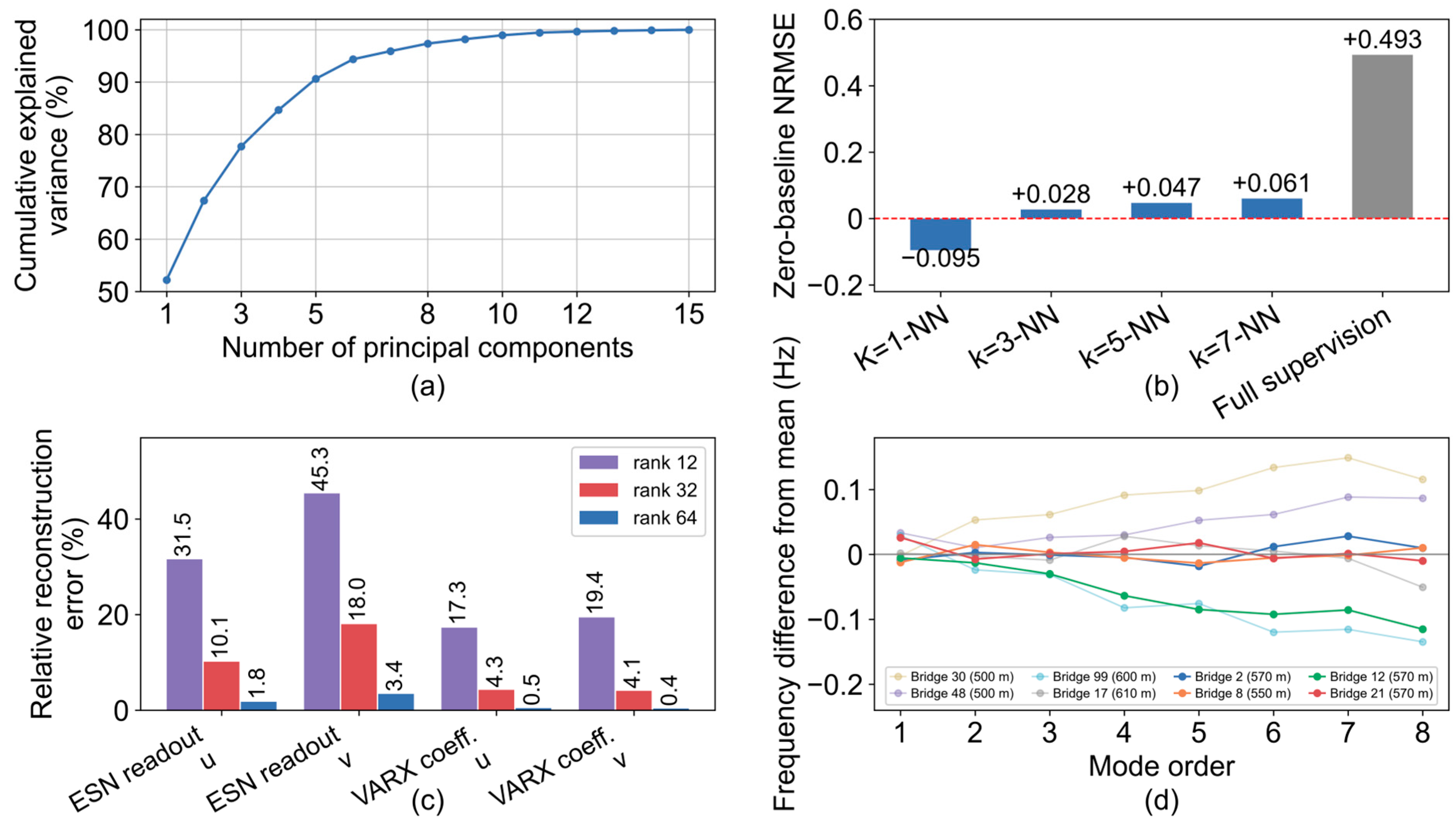
The ideal setting is zero-motion: to obtain a new bridge’s response model from its macroscopic design parameters alone. This section explains why this route is difficult from four angles (Figure 6): The four panels show the (a) PCA of the theta parameters; (b) k-nearest-neighbor transfer with the matched full-supervision reference; (c) low-rank reconstruction error; and (d) natural-frequency discrepancy relative to the across-bridge mean at each mode order.

Figure 6. Four aspects of the difficulty of direct transfer: (a) PCA of θ parameters; (b) k-NN transfer; (c) low-rank reconstruction error; (d) natural-frequency discrepancy.

The four steps that follow form a single argument. Section 4.1 first shows that zero-motion direct transfer is ineffective, ruling out the cheapest route; Section 4.2 then measures how accuracy grows with the number, K, of calibration motions, establishing whether a small number of motions can suffice; Section 4.3 shows that motions differ greatly in calibration quality, so that the problem is one of motion quality rather than quantity; and Section 4.4, consequently, designs the calibration excitation by inversion instead of selecting it. Each step supplies the necessity for the next.

(1)

A bridge is described by 15 macroscopic parameters, of which five are decisive. The full set contains 15 design quantities (main span, side span, tower height above and below deck, cables per tower side, cable spacing, girder dead load, girder area, girder flexural inertia, tower dead load, tower area, tower flexural inertia, lane number, cable tensile strength, and cable safety factor). Principal component analysis shows that the first five components explain 90.6% of the parameter variance and the first eight 97.4% (Figure 6a). These five summarize the bridge’s scale and stiffness, mainly span, tower height, girder load, tower stiffness, and cable safety factor. The parameter space is low-dimensional, but the mapping from macroscopic parameters to structural dynamics and the response model is not continuous: a few parameters fix the scale and dominant stiffness, yet not the detailed arrangement to which the response is highly sensitive. Parameters alone, therefore, cannot recover the response or its model.

(2)

Nearest-neighbor transfer fails. If similar parameters meant similar models, the closest trained bridge’s model could be moved directly to the new bridge. With k-nearest-neighbor transfer in the 15-dimensional parameter distance (Figure 6b), 1-NN results in an overall Zero-baseline NRMSE of only −0.095, worse than an all-zero prediction, and even k = 7 reaches only +0.061, about 15% of full supervision. The transferable commonality between bridges is, thus, very limited.

(3)

Model parameters are hard to share between bridges. Low-rank decomposition of the parameters of the 100 bridges (Figure 6c) shows that the VARX coefficients are fairly similar across bridges, with about 4% reconstruction error using the first 32 common directions, whereas the ESN readout differs much more, still 10% (u)/18% (v) at 32 directions and only below 2–3% beyond 64. The loss, thus, falls on the part that determines nonlinear prediction, as further confirmed when sharing readouts directly degrades accuracy to +0.009. This conclusion is limited to the low-rank decomposition and sharing scheme used here; better parameter-sharing routes may still exist.

(4)

The modal space of a structure depends on the detailed arrangement of stiffness and mass, which macroscopic parameters cannot fix. In Figure 6d, the first eight natural frequencies are plotted as differences from the across-bridge mean at each mode order for four bridges with the same main span of 550–570 m but different other parameters; the deviations reach about 0.12 Hz, with the first longitudinal floating frequency at 0.116–0.154 Hz and some 4–8th higher-order vertical bending modes up to 0.12 Hz below the mean.

Structural parameters alone are, therefore, insufficient to determine a new bridge’s response; the amplitude and spectral characteristics of the calibration excitation are equally key.

4.2. Performance of Few-Motion Calibration Versus K

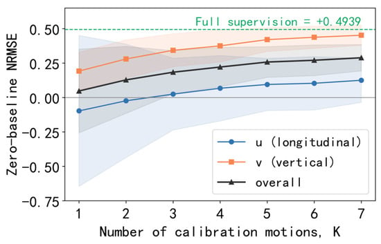
Since zero-motion direct transfer is difficult, the accuracy achievable by computing K motions for a new bridge is examined. In the experiment, K training motions are randomly drawn for a new bridge for nonlinear time-history computation, repeated 30 times and averaged, retraining only the readout of a plain ESN and evaluating on 10 test motions. Figure 7 shows the performance growth with K (shaded area: standard deviation across draws):

Figure 7. Performance of few-motion calibration versus, K (averaged random motions).

Figure 7 shows that the mean calibration score increases with the number of randomly selected motions, K. Each additional motion requires one target-bridge NLTHA. Section 4.3 examines how motion selection improves the score at a given K.

4.3. Good and Poor Motions: Representativeness of the Calibration Motion

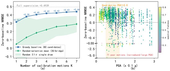
Given the freedom of motion selection, a key question is whether a single good motion can complete the new-bridge calibration. This is examined using an oracle-greedy procedure. The 80 training motions form the candidate pool. Each candidate alone trains an ESN readout, which is scored by the Zero-baseline NRMSE on the 10 validation motions to pick the best. Then, round by round, the selected set is fixed and the remaining candidates are jointly trained and re-scored to pick the single most effective motion. The K selected motions finally train the readout, evaluated independently on the 10 test motions.

Figure 8a shows that greedy selection improves calibration accuracy relative to random selection at the same number of motions. The effectiveness of the calibration records, therefore, matters in addition to their number, motivating the design of a dedicated calibration excitation.

Figure 8. Calibration-motion selection: (a) oracle-greedy versus random selection; (b) single-motion calibration score versus calibration-record PGA.

Figure 8b relates the single-motion calibration score to the PGA of the calibration record. The reported Spearman correlations are −0.21 with PGA and +0.02 with spectral flatness. The high-scoring calibration motions cluster around 0.07–0.09 g, approximately 0.7–0.9 on the plotted abscissa (units of 0.1 g). These observations motivate a calibration excitation that covers the low-frequency longitudinal motion and higher-frequency in-plane response, with sustained broadband input and moderate amplitude.

4.4. From Motion Selection to Motion Design: The Synthetic Calibration Motion (SCM)

The above analysis shows that new-bridge calibration can be achieved by selecting good motions, since one greedy-selected good motion matches more than ten randomly selected ones. This section turns motion selection into motion design: with surrogate prediction accuracy as the objective, a 60 s SCM is inversely designed so that a new bridge finishes surrogate calibration with one nonlinear time-history computation.

4.4.1. Design Rationale: Three Parameterizable Structures of a Good Motion

Starting from deterministic synthetic motions, five rounds of iteration reach a feasible formulation. Comparing Zero-baseline NRMSE: the logarithmic sweep (−0.42) and flat sweep (−0.97) are too regular and are overfit by the ESN, failing on random-phase real motions; the stationary band-pass white noise (−0.21) has the correct spectrum but no non-stationary envelope; adding the random phase and non-stationary envelope (+0.04) turns the performance positive for the first time; and amplitude leveling adds a large further gain (+0.25). The random phase and non-stationary envelope are, thus, the key.

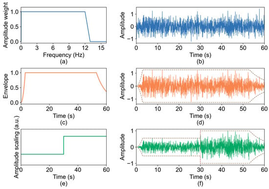
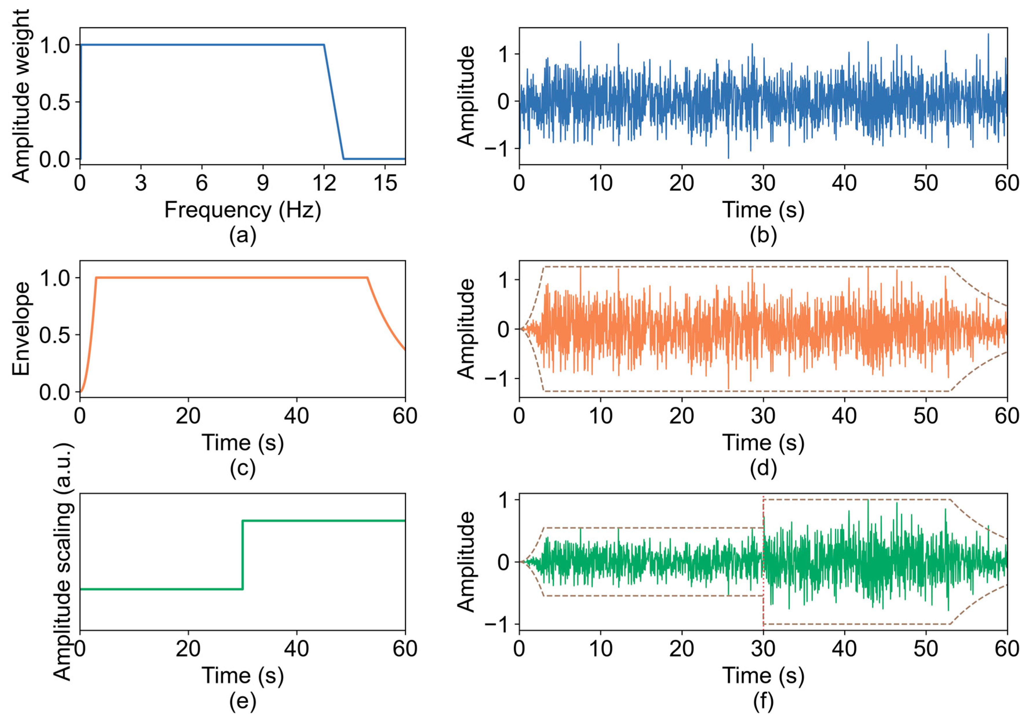
A good motion can, therefore, be decomposed into three parameterizable structures (Figure 9):

Figure 9. Three-structure decomposition of the SCM: (a) spectral weight; (b) broadband motion; (c) envelope; (d) enveloped motion; (e) amplitude scaling; (f) SCM-60 motion.

(1)

Spectral structure: the random phase keeps the motion’s statistical diversity consistent with real seismic records, and the broadband excites the low-frequency longitudinal floating mode and the high-frequency higher-order vertical bending modes at once.

(2)

Temporal envelope: An earthquake-like non-stationary envelope of a rise segment, a strong-motion plateau, and an exponential decay. The energy release of real earthquakes is non-stationary, and the envelope supplies this temporal structure.

(3)

Amplitude leveling: The amplitude is set segment by segment within one motion. The equivalent damping of the dampers and the bearing depends strongly on amplitude, so one leveled motion covers the linear, weakly nonlinear, and strongly nonlinear regions simultaneously.

4.4.2. SCM Parameter Analysis and Recommended Formulation

A strict single-factor sweep is then performed at a fixed seed (7) on three representative bridges. Each design changes exactly one factor: duration, amplitude leveling, PGA, bandwidth or envelope shape, with all others fixed at the standard design (60 s, 0.05–12 Hz, envelope 3/50/7 s, two-level leveling 0.6/1.1, and PGA 0.1 g); the seed is treated as a separate factor. Table 6 reports, for every design, the mean +/− sample SD over the three bridges. The mean score changes little with duration, remaining between +0.470 and +0.503, while the sample SD falls from 0.037 at 20 s to 0.012 at 100 s; 60 s was, therefore, chosen as a compromise between stability and cost. Two-level leveling is adequate: no leveling is clearly worse, while the 3-, 4- and 5-level variants produce similar results. The score is highest at a PGA of 1.0 × 0.1 g and falls by about 0.04 at 1.2–1.4 × 0.1 g. The lower frequency limit is a hard constraint, since raising it to 0.2 Hz collapses the accuracy, whereas 12 Hz already performs well at the upper end. The envelope shape matters little. The seed, by contrast, is the largest single source of variation, 0.312 to 0.524, and is, therefore, examined separately.

Table 6. All designs of the parameter sweep.

No.	Duration (s)	Amplitude Leveling	PGA (×0.1 g)	Bandwidth (Hz)	Envelope (s)	Seed	Overall (Mean ± SD)
1	20	2 levels 0.6/1.1	1.0	0.05–12	3/10/7	7	0.475 ± 0.037
2	40	2 levels 0.6/1.1	1.0	0.05–12	3/30/7	7	0.492 ± 0.109
3	60	2 levels 0.6/1.1	1.0	0.05–12	3/50/7	7	0.475 ± 0.025
4	80	2 levels 0.6/1.1	1.0	0.05–12	3/70/7	7	0.470 ± 0.016
5	100	2 levels 0.6/1.1	1.0	0.05–12	3/90/7	7	0.503 ± 0.012
6	60	no leveling	1.0	0.05–12	3/50/7	7	0.432 ± 0.041
7	60	4 levels 0.5/0.7/0.9/1.1	1.0	0.05–12	3/50/7	7	0.423 ± 0.061
8	60	3 levels 0.5/0.8/1.1	1.0	0.05–12	3/50/7	7	0.418 ± 0.057
9	60	5 levels 0.4/0.6/0.8/1.0/1.2	1.0	0.05–12	3/50/7	7	0.427 ± 0.047
10	60	2 levels 0.6/1.1	0.8	0.05–12	3/50/7	7	0.443 ± 0.015
11	60	2 levels 0.6/1.1	1.2	0.05–12	3/50/7	7	0.435 ± 0.028
12	60	2 levels 0.6/1.1	1.4	0.05–12	3/50/7	7	0.432 ± 0.038
13	60	2 levels 0.6/1.1	1.0	0.1–12	3/50/7	7	0.415 ± 0.031
14	60	2 levels 0.6/1.1	1.0	0.2–12	3/50/7	7	0.202 ± 0.084
15	60	2 levels 0.6/1.1	1.0	0.05–8	3/50/7	7	0.379 ± 0.070
16	60	2 levels 0.6/1.1	1.0	0.05–15	3/50/7	7	0.429 ± 0.041
17	60	2 levels 0.6/1.1	1.0	0.05–12	2/52/6	7	0.435 ± 0.026
18	60	2 levels 0.6/1.1	1.0	0.05–12	4/48/8	7	0.434 ± 0.027
19	60	2 levels 0.6/1.1	1.0	0.05–12	5/47/8	7	0.430 ± 0.032
20	60	2 levels 0.6/1.1	1.0	0.05–12	3/50/7	23	0.440 ± 0.018
21	60	2 levels 0.6/1.1	1.0	0.05–12	3/50/7	77	0.312 ± 0.154
22	60	2 levels 0.6/1.1	1.0	0.05–12	3/50/7	101	0.488 ± 0.053
23	60	2 levels 0.6/1.1	1.0	0.05–12	3/50/7	202	0.435 ± 0.037
24	60	2 levels 0.6/1.1	1.0	0.05–12	3/50/7	303	0.485 ± 0.015
25	60	2 levels 0.6/1.1	1.0	0.05–12	3/50/7	404	0.524 ± 0.052
26	60	2 levels 0.6/1.1	1.0	0.05–12	3/50/7	505	0.500 ± 0.061

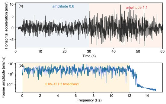
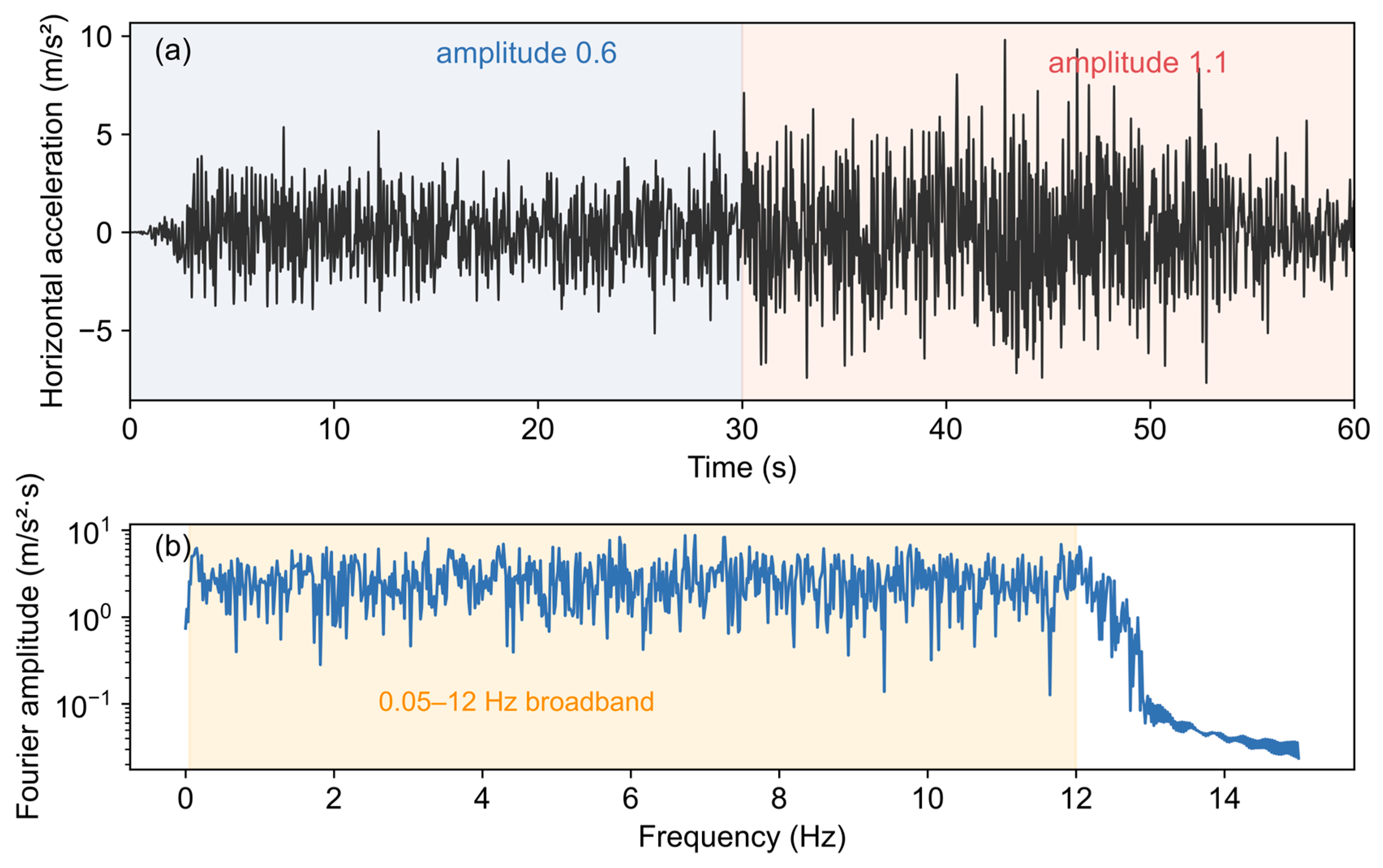
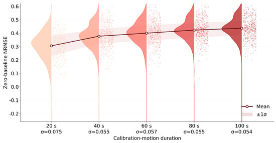
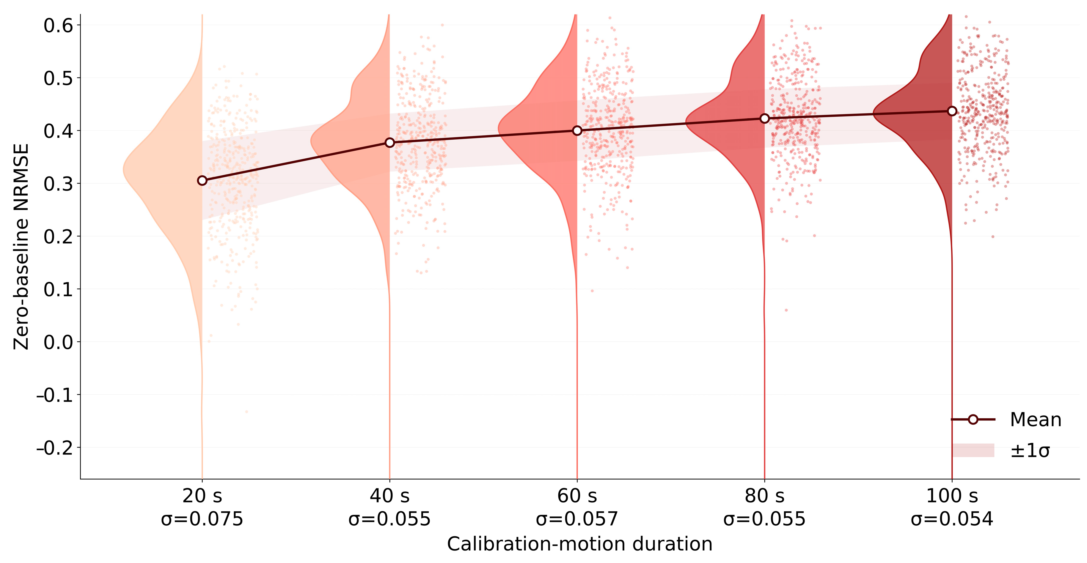
The final formulation is, therefore, SCM-60 (Figure 10): a random-phase broadband of 0.05–12 Hz, a non-stationary envelope with a 3 s rise, 50 s strong motion and 7 s decay, a two-level amplitude scaling of 0.6 and 1.1, a PGA of 0.1 g, a total duration of 60 s and a time step of 0.02 s. The seed effect is traced to phase differences that change the arrival time and effective duration of the long-period components: at 20 s, the longitudinal drift mode is under-excited (the pooled within-bridge σ is 0.075), whereas at 60 s, the excitation becomes adequate and σ falls to 0.057.

Figure 10. SCM-60: (a) time history; (b) amplitude spectrum.

The vertical component is an independent random-phase realization with the same spectral band, envelope and amplitude grading, scaled to 0.65 times the horizontal peak, and is applied simultaneously with the horizontal component.

The parameter sweep leads to the SCM-60 formulation described above.

The bandwidth is chosen from the parameter sweep in Table 6. Raising the upper limit from 12 to 15 Hz lowers the three-bridge average from +0.475 to +0.429, and compressing it to 8 Hz lowers it to +0.379, so 12 Hz already performs well at the upper end. Raising the lower limit from 0.05 to 0.1 Hz yields +0.415, and raising it to 0.2 Hz collapses the average to +0.202; lowering the limit from 0.1 to 0.05 Hz is, therefore, still worth 0.06. The recommended bandwidth is, therefore, 0.05–12 Hz, which maintains a safe margin at the low-frequency end.

Figure 11 shows the 420 bridge–seed scores at each duration: 21 blind-test bridges × 20 seeds, with each score averaged over ten test motions. The violins show the pooled distribution; the dark line shows its mean, and the shaded band shows ±1 pooled within-bridge standard deviation across seeds. From 20 to 60 s, the mean increases from 0.305 to 0.400, and the pooled within-bridge standard deviation decreases from 0.075 to 0.057. At 100 s, these values are 0.437 and 0.054. The SCM-60 balances calibration duration, prediction score and seed sensitivity.

Figure 11. Seed-to-seed variability of the SCM Zero-baseline NRMSE versus calibration-motion duration.

4.4.3. Development-Bridge Validation and Independent Blind Testing

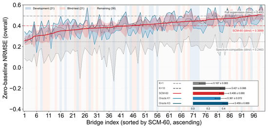
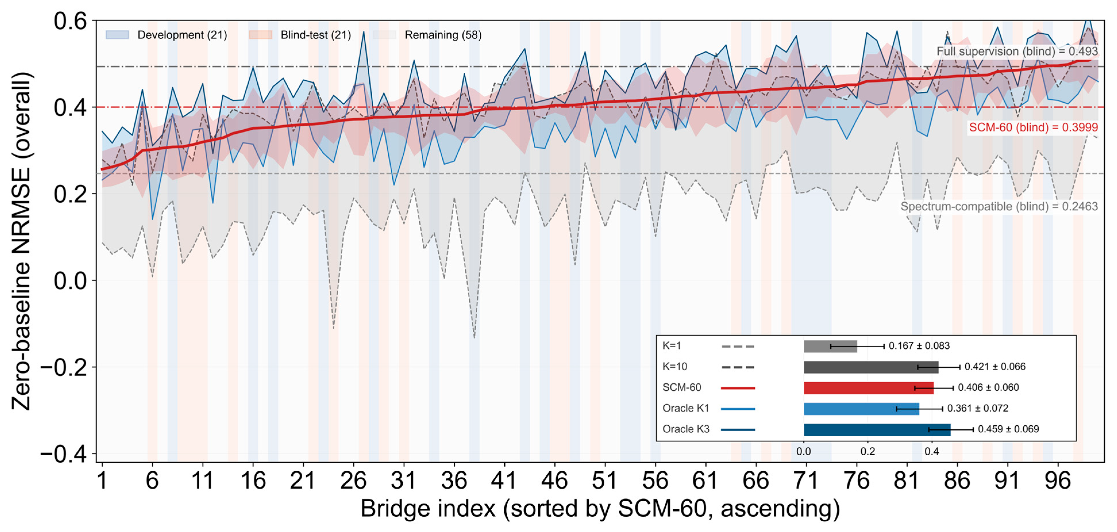
The SCM formulation was developed using 21 development bridges and frozen before evaluation on a separate set of 21 blind-test bridges. On the development bridges, SCM-60 results in an overall Zero-baseline score of 0.424 and a Peak-normalized score of 0.932. On the blind-test bridges, 20 seeds produces 420 bridge–seed scores, each averaged over the same ten test motions. The pooled Zero-baseline score is 0.400 ± 0.084, and every bridge has a positive seed-averaged score. The matched full-supervision model, using 80 training records and the same blind bridges, response nodes and test motions, yields 0.4934 ± 0.082, with a Peak-normalized score of 0.940. The SCM mean is approximately 81% of this matched Zero-baseline reference. Figure 12 extends the per-bridge comparison to all 100 bridges, using the 20-seed SCM-60 average for each bridge.

Figure 12. Per-bridge Zero-baseline NRMSE for all 100 bridges.

SCM-60 is the 20-seed average of the 60 s computations; K = 1 and K = 10 are random-selection baselines computed for all 100 bridges; Oracle K1 and Oracle K3 are the greedy-selected one- and three-motion calibrations, computed for all 100 bridges from the same 80-motion candidate pool. The horizontal dash-dot lines mark the blind-bridge means of the full-supervision model and of SCM-60, respectively.

Across the 100 bridges in Figure 12, the mean Zero-baseline scores are 0.406 for one SCM, 0.167 for one randomly selected motion and 0.421 for ten randomly selected motions. One SCM, therefore, approaches the ten-motion random-calibration result using one target-bridge analysis. Oracle K1 and Oracle K3 give 0.361 and 0.459, respectively, on the same 100-bridge summary. For the 21 blind bridges, the SD of the bridge mean scores is 0.064, the pooled within-bridge SD across seeds is 0.057, and the SD of all 420 bridge–seed scores is 0.084. These quantities describe different sources of variation. A spectrum-compatible selection baseline results in a blind-bridge mean of 0.246, compared with 0.400 for SCM-60.

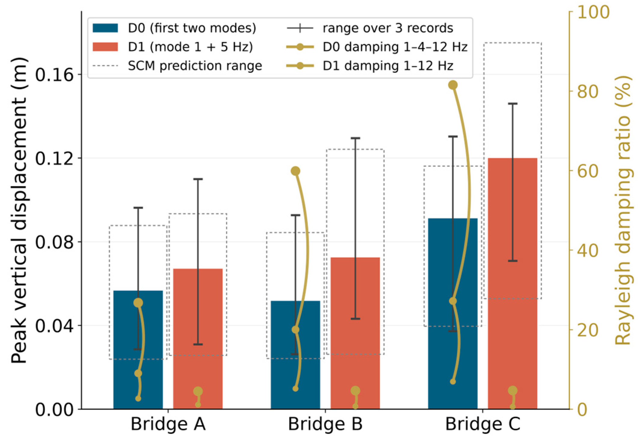
Figure 13 compares the baseline Rayleigh calibration D0, anchored at the first two modes, with D1, anchored at the first mode and 5 Hz. D0 results in damping ratios of approximately 27–82% between 4 and 12 Hz, attenuating the response to the upper part of the SCM input band. Under D1, the mean peak vertical displacement increases by approximately 18%, 40% and 32% for bridges A, B and C. The SCM-calibrated prediction ranges also shift upward with the same trend and still bracket the measured peaks, so the ranking of the bridges and the longitudinal/vertical contrast are unchanged. In the figure, bars are the mean over the three real records and whiskers the record-to-record range, dashed boxes are the ranges predicted by the SCM-calibrated surrogate, and the yellow dots and curves on the right axis give the Rayleigh damping ratio at 1, 4 and 12 Hz for D0 and at 1 and 12 Hz for D1; A, B and C denote the small- (240 m), medium- (500 m) and large-span (820 m) bridges.

Figure 13. Sensitivity of the peak vertical deck displacement to the Rayleigh damping calibration.

4.4.4. Applying SCM to a New Bridge

A new bridge is calibrated by one NLTHA under SCM-60. The leading p = 12 right singular vectors of this response define the spatial basis, and the readout is fitted to the same response with λ = 300. Both constants are fixed before application to the new bridge. Target accelerations are normalized by the calibration RMS, passed through the reservoir and mapped back to nodal displacements. Duration scaling of Table 5 yields estimated calibration-analysis times of 95, 151 and 644 s for the small, medium and large span classes. Basis extraction and readout fitting use the stored calibration response. Table 5 presents the prediction times, and Appendix A specifies the algorithm.

5. Limitations and Outlook

The accuracy and computational benefits are established for the 100-record benchmark with horizontal PGA up to 0.29 g. The SCM obtains the calibration data by designing one excitation for a new bridge. This approach complements transfer-learning methods such as that of Han et al. [15], which adapt a pretrained surrogate using target-bridge responses.

The surrogate predicts longitudinal and vertical nodal displacement histories. Member forces, cable forces, stress, strain, damage indices, torsion and out-of-plane response are not evaluated as surrogate outputs. The comparison includes neither LSTM nor an equivalent-linear-device baseline.

Future work will combine SCM with transfer learning and physical constraints, extend it to other bridge forms and excitation types, and integrate calibration-motion design with code-based motion selection.

6. Conclusions

The study develops a universal SCM for calibrating the seismic-response surrogate of a new cable-stayed bridge. The following conclusions on prediction accuracy and computational benefits concern the 100-bridge benchmark and analyzed ground-motion windows with horizontal PGA up to 0.29 g:

(1)

Among the eleven surrogate methods, the nonlinear-readout models perform best: ESN and VR-ESN reach the highest overall scores, and both return a response prediction in sub-second time. The linear family behaves very differently. The physical linear baselines, modal superposition and the H1 transfer function, fail on these strongly nonlinear responses and yield negative scores, because they cannot represent the hysteretic devices. The linear VARX family and the FIR filter recover part of the response, but their accuracy saturates well below that of the nonlinear readout, and raising the model order brings only diminishing returns. Blending linear submodels improves on the individual components by a small margin only, and the gain comes from the residual learned by the nonlinear readout rather than from the linear part.

(2)

The four analyses, covering zero-motion transfer, few-motion calibration, motion selection and motion design, show that in this database the seismic response of a long-span cable-stayed bridge is governed by the detailed arrangement of stiffness and mass rather than by its macroscopic parameters alone. The fifteen design parameters fix the scale and the dominant stiffness, yet they do not fix the modal space, and the model parameters that control the nonlinear response cannot be transferred between bridges. The response of a new bridge is, therefore, obtained through calibration motions rather than through its parameters, and the quality of those motions, not their number, sets how much the calibration can achieve.

(3)

The calibration excitation can be designed rather than selected. A 60 s SCM combines a randomized-phase broadband of 0.05–12 Hz; a non-stationary envelope of 3 s rise, 50 s strong motion and 7 s decay; a two-level amplitude grading of 0.6 and 1.1; and a horizontal PGA of about 0.1 g. One NLTHA under this motion supplies both the spatial basis and the readout targets, and later predictions take sub-second time. This is one effective parameter combination rather than a unique optimum: the parameter sweep shows that several neighboring settings reach similar accuracy, and part of the parameters can be fine-tuned without changing the main conclusions. For a medium bridge, a 200-analysis IDA costs about 2.8 h and a 1000-sample fragility analysis about 14 h, against about 1.3 min and 2 min with SCM, i.e., factors of about 130 and 430 within the range examined here.

(4)

With one universal SCM, a new bridge is calibrated by a single target-bridge NLTHA and reaches about 81% of the matched full-supervision score obtained with 80 motions. Across all 100 bridges, its accuracy comes close to that of ten randomly selected calibration motions and lies between the one- and three-motion results of a greedy selection over the 80-motion candidate pool.

References

- Löhning, T.; Ravn, U.G.; Pedersen, F.; Westh, L.; Christoffersen, M. The 1915 Çanakkale Bridge—Design and Construction of Substructure. In Proceedings of the IABSE Symposium, Istanbul, Turkey, 26–28 April 2023; pp. 575–582. [Google Scholar]
- Karoumi, R. Some modeling aspects in the nonlinear finite element analysis of cable supported bridges. Comput. Struct. 1999, 71, 397–412. [Google Scholar] [CrossRef] [Scilit]
- Chen, X.; Kareem, A. Revisiting multimode coupled bridge flutter: Some new insights. J. Eng. Mech. 2006, 132, 1115–1123. [Google Scholar] [CrossRef] [Scilit]
- Song, L.; Fan, J.; Zeng, S.; Wang, C. Frontier AI in computational civil engineering: A review of graph, sequence, physics-informed deep learning, and beyond (2020–2025). Smart Constr. 2026, 1, 1–49. [Google Scholar] [CrossRef] [Scilit]
- Song, L.; Wang, C.; Fan, J. Efficient full-range nonlinear analyses of structural systems based on heterogeneous graph learning. Engineering 2026, 59, 320–336. [Google Scholar] [CrossRef] [Scilit]
- Zhang, C.; Tao, M.; Wang, C.; Fan, J.-S. Differentiable automatic structural optimization using graph deep learning. Adv. Eng. Inform. 2024, 60, 102363. [Google Scholar] [CrossRef] [Scilit]
- Wang, C.; Zhang, C.; Yang, C.; Fan, J.-S. Towards efficient structural inverse analysis based on AI-driven differentiable optimization method. Mech. Syst. Signal Process. 2025, 230, 112618. [Google Scholar] [CrossRef] [Scilit]
- Chen, P.; Wang, C.; Fan, J. Multivariate engineering formulas discovery with knowledge-based neural network. Comput. Aided Civ. Infrastruct. Eng. 2025, 16, e13448. [Google Scholar]
- Liu, Y.; Lu, N.; Yin, X.; Noori, M. An adaptive support vector regression method for structural system reliability assessment and its application to a cable-stayed bridge. Proc. Inst. Mech. Eng. Part O J. Risk Reliab. 2016, 230, 204–219. [Google Scholar] [CrossRef] [Scilit]
- Zhang, X.; Han, Y.; Wang, L.; Liu, H.; Cai, C. An adaptive surrogate model approach for random vibration analysis of the train–bridge system. Eng. Struct. 2023, 278, 115490. [Google Scholar] [CrossRef] [Scilit]
- Wang, L.; Zhang, X.; Han, Y.; Liu, H.; Hu, P.; Cai, C. A fast hybrid algorithm for the random vibration analysis of train-bridge systems under crosswinds. Eng. Struct. 2024, 299, 117107. [Google Scholar] [CrossRef] [Scilit]
- Zhang, X.; Wang, L.; Han, Y.; Xu, G.; Cai, C.; Liu, H. An efficient method for predicting wheel-rail forces in coupled nonlinear train-track-bridge system using artificial neural networks. Adv. Struct. Eng. 2023, 26, 1228–1241. [Google Scholar] [CrossRef] [Scilit]
- Shen, Y.; Ma, G.; Hwang, H.J.; Kim, D.J.; Zhang, Z. Prediction of seismic response of building structures using a CNN-LSTM-ATT network with transfer learning. Adv. Struct. Eng. 2025, 28, 2710–2725. [Google Scholar] [CrossRef] [Scilit]
- Liu, Q.; Liu, Z.; Zhao, J.; Lei, Y.; Zhu, S.; Wu, X. Seismic Optimization of Fluid Viscous Dampers in Cable-Stayed Bridges: A Case Study Using Surrogate Models and NSGA-II. Buildings 2025, 15, 1446. [Google Scholar] [CrossRef] [Scilit]
- Han, Z.; She, D.; Liu, J. A Transfer Learning-Based Hybrid Surrogate Modeling Framework for Efficient Multi-Objective Seismic Design of Long-Span Cable-Stayed Bridges. Buildings 2026, 16, 904. [Google Scholar] [CrossRef] [Scilit]
- Yin, X.; Huang, Z.; Liu, Y. Bridge damage identification under the moving vehicle loads based on the method of physics-guided deep neural networks. Mech. Syst. Signal Process. 2023, 190, 110123. [Google Scholar] [CrossRef] [Scilit]
- Huang, Z.; Yin, X.; Liu, Y. Physics-guided deep neural network for structural damage identification. Ocean Eng. 2022, 260, 112073. [Google Scholar] [CrossRef] [Scilit]
- Jin, Z.; Pei, S.; Wei, X.; Liu, H.; Qiang, S. Partially earth-anchored cable bridge: Ultralong-span system suitable for carbon-fiber-reinforced plastic cables. J. Bridge Eng. 2016, 21, 06016003. [Google Scholar] [CrossRef] [Scilit]
- Kawada, T.; Ohashi, H.; Scott, R. History of the Modern Suspension Bridge: Solving the Dilemma between Economy and Stiffness; ASCE: Reston, VA, USA, 2010. [Google Scholar]
- Maekawa, K.; Morizono, Y.; Nakamura, K.; Eguchi, T.; Fujino, Y. Structural characteristics and economical efficiency of an ultra long-span suspension bridge using new material (FRP) cable. J. Struct. Eng. JSCE 2000, 46, 1343–1352. [Google Scholar]
- Meier, U. Proposal for a carbon fibre reinforced composite bridge across the Strait of Gibraltar at its narrowest site. Proc. Inst. Mech. Eng. Part B 1987, 201, 73–78. [Google Scholar] [CrossRef] [Scilit]
- Dong, L.; Feng, P.; Lu, C.; Zhang, P.; Ding, G. Rapid design for large-scale parallel CFRP cable with multi-source experimental data. Eng. Struct. 2024, 305, 117771. [Google Scholar] [CrossRef] [Scilit]
- Dong, L.; Feng, P. CFRP–cable-stayed bridge hybrid with partial suspension and a span exceeding 3000 m: Concept, optimization, and construction. J. Bridge Eng. 2025, 30, 04025050. [Google Scholar] [CrossRef] [Scilit]
- Yang, Y.; Wang, X.; Wu, Z. Evaluation of the static and dynamic behaviors of long-span suspension bridges with FRP cables. J. Bridge Eng. 2016, 21, 06016008. [Google Scholar] [CrossRef] [Scilit]
- Xiong, W.; Cai, C.S.; Zhang, Y.; Xiao, R. Study of super long span cable-stayed bridges with CFRP components. Eng. Struct. 2011, 33, 330–343. [Google Scholar] [CrossRef] [Scilit]
- Li, C.; Zhang, C.; Li, S.; Chen, Y.; Zhai, C. Transfer learning-enhanced surrogate model for the prediction of structural full-profile seismic time-history response. J. Build. Eng. 2025, 116, 114714. [Google Scholar] [CrossRef] [Scilit]
- Ponce-Lopez, E.; Yanez-Godoy, H. A machine learning-based surrogate model for analyzing the nonlinear seismic response of steel moment frames with rotational friction dampers. Mach. Learn. Appl. 2026, 26, 101030. [Google Scholar] [CrossRef] [Scilit]
- Liang, Y.; Liu, Y.; Zhang, K.; Kong, Y.; Guan, P. Seismic fragility analysis of single-pylon double-plane highway cable-stayed bridge. Struct. Concr. 2026, 27, 8358–8373. [Google Scholar] [CrossRef] [Scilit]
- Nav, F.M.; Snaiki, R. Time-domain buffeting response prediction of a long-span bridge: A hybrid machine learning framework. Structures 2025, 73, 108286. [Google Scholar] [CrossRef] [Scilit]
- Li, Y.; Sun, Z.; Mangalathu, S.; Li, Y.; He, W.; Xue, X. Machine learning-based full-life-cycle seismic response assessment for in-service bridge piers: Comprehensive analysis of interpretability and seismic fragility. Structures 2025, 80, 110050. [Google Scholar] [CrossRef] [Scilit]
- Luo, L.; Li, Y.; Dai, H.; Sun, H.; Jia, M.; Yuan, H.; Cheng, X. Seismic performance prediction and interpretation of RC bridges under vehicle-bridge interaction: From VBI system simulation to ensemble learning surrogate models. Eng. Struct. 2025, 341, 120816. [Google Scholar] [CrossRef] [Scilit]
- Shao, Z.; Peng, X.; Zhang, P.; Liu, Z.; Chen, Y.; Yang, R.; Xiang, P. An intelligent GNN seismic response prediction and computation framework adhering to meshless principles: A case study for high-speed railway bridges. Eng. Anal. Bound. Elem. 2025, 179, 106359. [Google Scholar] [CrossRef] [Scilit]
- Guo, W.; He, Y.; Hu, Y.; Xu, Z. Transfer learning-enhanced neural networks for seismic response prediction of high-speed railway simply supported bridges. Soil Dyn. Earthq. Eng. 2025, 191, 109228. [Google Scholar] [CrossRef] [Scilit]
- Goswami, S.; Giovanis, D.G.; Li, B.; Spence, S.M.J.; Shields, M.D. Neural operators for stochastic modeling of nonlinear structural system response to natural hazards. Eng. Struct. 2025, 345, 121284. [Google Scholar] [CrossRef] [Scilit]
- Kim, J.; Yi, S.-r.; Wang, Z. A composition of simplified physics-based model with neural operator for trajectory-level seismic response predictions of structural systems. Struct. Saf. 2026, 119, 102668. [Google Scholar] [CrossRef] [Scilit]
- Chen, R.; Zhou, T.; Pan, H.; Kim, C.-W. Attention-enhanced Fourier neural operator for stochastic seismic response analysis and reliability assessment. Struct. Saf. 2026, 122, 102722. [Google Scholar] [CrossRef] [Scilit]
- Yadav, M.; Chauhan, S.; Shrimali, M.D.; Stender, M. Predicting multi-parametric dynamics of an externally forced oscillator using reservoir computing and minimal data. Nonlinear Dyn. 2025, 113, 5977–5990. [Google Scholar] [CrossRef] [Scilit]
- Yan, Y.; Xie, Y.; Xia, Y.; Sun, L. Systematic investigation on surrogate and active learning-based multivariate seismic fragility analysis under multiple sources of uncertainties. Reliab. Eng. Syst. Saf. 2026, 265, 111588. [Google Scholar] [CrossRef] [Scilit]
- Kim, J.; Su, M.; Wang, Z.; Broccardo, M. Recorded versus synthetic spectral-compatible ground motions: A comparative analysis of structural seismic responses. Earthq. Eng. Struct. Dyn. 2026, 55, 827–843. [Google Scholar] [CrossRef] [Scilit]
- Chen, C.; Ma, Y.; Yan, D.; Li, Z. Coupled nonlinear and time-dependent analysis for long span cable-stayed bridges. Struct. Infrastruct. Eng. 2020, 16, 1416–1429. [Google Scholar] [CrossRef] [Scilit]
- Sun, Y.; Zhan, Y.; Huang, Y.; Wang, Y.; Shao, J.; Chen, X.; Ling, X.; Li, Y. Research on seismic performance optimization of cable-stayed bridge dampers based on machine learning. Adv. Bridge Eng. 2026, 7, 4. [Google Scholar] [CrossRef] [Scilit]
- Xiao, Z.; Huang, S.; Li, S.; Li, M.; Hu, Y. Low-damage seismic design approach for a long-span cable-stayed bridge in a high seismic hazard zone: A case study of the New Panama Canal Bridge. Buildings 2026, 16, 428. [Google Scholar] [CrossRef] [Scilit]
- Ancheta, T.D.; Darragh, R.B.; Stewart, J.P.; Seyhan, E.; Silva, W.J.; Chiou, B.S.J.; Wooddell, K.E.; Graves, R.W.; Kottke, A.R.; Boore, D.M.; et al. NGA-West2 Database. Earthq. Spectra 2014, 30, 989–1005. [Google Scholar] [CrossRef] [Scilit]
- Zhang, Z.; Zeng, Z.; Wei, G.; Zhang, Y. Stochastic response and dynamic reliability analysis of long-span cable-stayed bridges under non-stationary ground motions via DPIM. Structures 2026, 84, 111050. [Google Scholar] [CrossRef] [Scilit]
Disclaimer/Publisher’s Note: The statements, opinions and data contained in all publications are solely those of the individual author(s) and contributor(s) and not of MDPI and/or the editor(s). MDPI and/or the editor(s) disclaim responsibility for any injury to people or property resulting from any ideas, methods, instructions or products referred to in the content. |
© 2026 by the authors. Licensee MDPI, Basel, Switzerland. This article is an open access article distributed under the terms and conditions of the Creative Commons Attribution (CC BY) license.