Real-Time Analysis of Concrete Placement Progress Using Semantic Segmentation

Abstract

Concrete arch dams represent a predominant dam type in water conservancy and hydropower projects in China. The control of concrete placement progress during construction directly impacts project quality and construction efficiency. Traditional manual monitoring methods, characterized by delayed response and strong subjectivity, struggle to meet the demands of modern intelligent construction management. This study introduces machine vision technology to monitor the concrete placement process and establishes an intelligent analysis system for construction scenes based on deep learning. By comparing the performance of U-Net and DeepLabV3+ semantic segmentation models in complex construction environments, the U-Net model, achieving an IoU of 89%, was selected to identify vibrated and non-vibrated concrete areas, thereby optimizing the concrete image segmentation algorithm. A comprehensive real-time analysis method for placement progress was developed, enabling automatic ternary classification and progress calculation for key construction stages, including concrete unloading, spreading, and vibration. In a continuous placement case study of Monolith No. 3 at a project site, the model’s segmentation results showed only an 8.2% error compared with manual annotations, confirming the method’s real-time capability and reliability. The research outcomes provide robust data support for intelligent construction management and hold significant practical value for enhancing the quality and efficiency of hydraulic engineering construction.

1. Introduction

Concrete arch dams are a critical dam type in China’s hydraulic engineering, whose construction quality directly impacts the structural safety and long-term stability of the project. As a core link of arch dam construction, the monitoring and management of placement progress at the construction face are essential for ensuring project quality. Traditional methods relying on manual inspections are inherently lagging and subjective, often failing to provide accurate real-time data support [1]. Given that arch dam construction involves continuous concrete placement, onsite constraints, and strict temperature control requirements, the process typically divides the dam body into multiple monoliths or placement blocks [2]. Quality control of concrete placement in each monolith is fundamental to the quality control of the entire dam construction [3]. The construction environment at the placement face involves numerous elements; effective coordination among materials, machinery, and personnel, coupled with timely feedback and adjustment, is central to ensuring placement quality [4]. Advances in deep learning and machine vision technologies have laid the groundwork for intelligent monitoring systems for placement operations [1,2].

As a core aspect of hydraulic engineering construction, the quality control of concrete dam construction has undergone a paradigm shift from manual supervision to intelligent perception. Early research primarily relied on empirical knowledge and process optimization. For instance, Jiang Weiqun’s team proposed a placement block design method based on thermal control parameters and aggregate gradation, enabling full-process manual supervision through standardized construction records, though without integrated automated monitoring modules. With the advancement of IoT technology, construction quality monitoring entered an automated phase. Wu Binping et al. [5] developed a full-process material tracking system that integrated mixing plant production data, transport vehicle trajectories, and cable crane operation logs, achieving closed-loop quality traceability from raw material preparation to concrete placement. In the field of positioning technology, Gong [6] employed Ultra-Wideband (UWB) positioning to reconstruct vibrator trajectories and evaluated compaction uniformity via spatiotemporal data analysis. Meanwhile, Tian’s [7] team integrated GPS/GLONASS dual-mode positioning with RTK phase enhancement technology, achieving centimeter-level accuracy and establishing dynamic correlation rules between vibration duration and area compaction density. Current research focuses on building intelligent quality evaluation systems. Wang Rui et al. [8] developed a rolling compaction quality prediction model based on a Multilayer Perceptron (MLP), enabling online compaction assessment through deep feature mapping of material properties and compaction parameters. Zhong innovatively proposed a cross-stage prediction framework linking vibration processes to concrete strength, using a random forest algorithm to model nonlinear relationships between parameters such as water–cement ratio and vibration depth versus compressive strength at design age. The model demonstrates significantly better correlation with measured data than conventional empirical formulas.

The environment at the placement face is highly dynamic and complex, characterized by factors such as haze, dust, variable illumination (from daylight to nighttime low light or artificial glare), and frequent occlusions from machinery and personnel. These challenges often lead to significant image quality degradation, including blur, low contrast, and noise. Under such non-ideal and fluctuating conditions, traditional visual recognition techniques—and even many standard deep learning models trained on clean benchmark datasets—struggle to perform reliably. They frequently fail to maintain both high segmentation accuracy and real-time inference speeds when confronted with persistent poor illumination or atmospheric interference [9]. This limitation directly hinders the robust, automated, and continuous assessment of critical construction states (e.g., distinguishing vibrated from non-vibrated concrete) and real-time progress tracking. Consequently, there exists a clear gap in vision-based monitoring systems that can deliver consistent, real-time performance under the realistic adversities of a construction site. Enhancing image preprocessing to counter quality degradation and advancing segmentation models for better accuracy-efficiency trade-offs are therefore pivotal to enabling practical and intelligent monitoring solutions.

Deep learning, particularly Convolutional Neural Networks (CNNs), has demonstrated significant advantages in image processing [10]. Compared to traditional methods reliant on handcrafted feature extraction, deep learning can autonomously learn complex features from large-scale data, offering higher recognition accuracy [11,12]. A deep learning-based model for identifying placement progress, when properly trained, can automatically distinguish between vibrated and non-vibrated concrete areas, providing accurate assessment of placement advancement. This study employed both U-Net and DeepLabV3+ semantic segmentation models, implemented with PyTorch (version 1.12.1), for training and testing on images from placement faces. Comparative analysis indicated that the U-Net model offers notable advantages in training speed and processing efficiency, whereas the DeepLabV3+ model exhibits stronger robustness in complex scenarios involving obstructions or cluttered backgrounds [4].

Semantic segmentation is a specific subfield of image segmentation focused on assigning each pixel in an image to a predefined semantic category, thereby achieving pixel-level segmentation and semantic labeling. With the rapid development of deep learning, semantic segmentation models have evolved from traditional methods to end-to-end architectures based on deep learning. Prior to CNNs, semantic segmentation primarily relied on traditional image processing techniques, such as graph theory-based Normalized Cut algorithms, or utilized handcrafted features (e.g., color, texture) alongside classifiers like Random Forests trained on textons. In 2014, the emergence of the Fully Convolutional Network (FCN) decomposed the semantic segmentation task into encoder and decoder components, marking the beginning of a period of rapid advancement [13]. Subsequent innovations include U-Net, which introduced a symmetric encoder–decoder structure significantly improving performance on small datasets; SegNet, which incorporated unpooling operations to reduce parameter count; RefineNet, which enhanced segmentation of small objects by fusing feature maps from different levels; DeepLab, which proposed atrous (dilated) convolutions to mitigate resolution loss from pooling operations [14,15,16]; and Mask R-CNN, which added an independent segmentation branch to existing object detection frameworks (bounding box regression and classification), enabling parallel detection and segmentation [17]. Driven by algorithmic and hardware progress, models based on these core innovations continue to evolve, serving unique roles across various domains and scenarios.

Addressing the objectives of this study, considering the limited field of view of onsite monitoring cameras (typically focused on specific monolith areas) resulting in relatively high image resolution, and the large scale of the core recognition target (concrete placement areas), which minimizes the need for small object detection, this research selected two advanced architectures: DeepLab v3+ for semantic segmentation and Mask R-CNN for instance segmentation [18]. These models were specifically applied to accurately identify and segment the core element in placement face scenes—concrete, particularly distinguishing its vibrated and non-vibrated states. The study systematically compared and evaluated the two models on key performance metrics—segmentation accuracy, robustness, and inference speed—within complex placement face environments (featuring partial occlusion by equipment, interference from personnel activity, varying lighting conditions, etc.), aiming to establish a reliable perceptual foundation for subsequent real-time progress analysis.

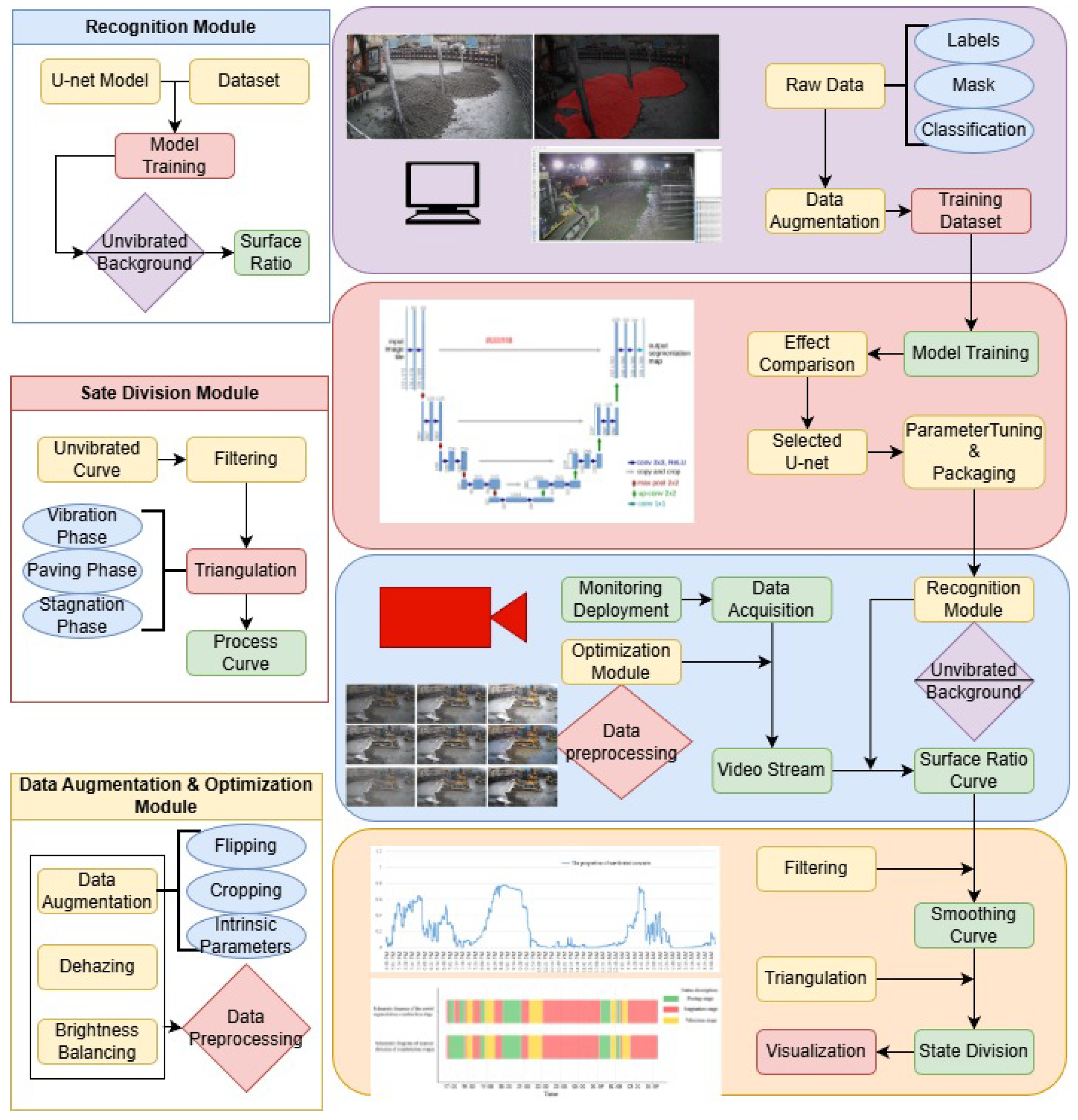
Building upon the high-precision semantic segmentation results of the concrete state (especially the vibration-completed areas) on the placement face, this study innovatively proposes a “real-time analysis method for full-cycle placement progress.” The core of this method lies in transcending the limitations of traditional static images or manual records, achieving continuous capture and quantitative analysis of the dynamic evolution of the placement process. Its key innovations are reflected in three aspects (seen in Figure 1):

(1)

Multi-stage State Perception and Fusion The method goes beyond assessing the concrete state at a single static moment. It systematically integrates the continuous semantic segmentation results from key construction phases (including unloading, spreading, and vibration). The segmentation results for each phase are assigned specific semantic labels and timestamps.

(2)

Temporal Modeling and Progress Quantification: The method innovatively incorporates time series analysis techniques to model the continuously acquired multi-stage segmentation results. By analyzing the spatial evolution patterns (e.g., area growth, boundary progression) of different state regions (particularly the “vibrated” areas) over time, it dynamically calculates and quantifies the real-time completion progress of each construction phase (e.g., vibration completion rate, unit placement completion rate) and tracks their change curves over time.

(3)

Dynamic Process Monitoring and Decision Support: Unlike traditional methods reliant on static snapshot evaluations, this approach enables real-time, dynamic capture of spatial distribution changes in the concrete state throughout the entire placement process, precisely analyzing the progress evolution from initial unloading to completed vibration for each step. The deep learning-based semantic segmentation model automatically identifies the concrete state at different time points. Combined with a temporal analysis engine, it accurately assesses the overall placement progress of the current monolith, the efficiency of sub-processes, and potential lagging segments. This provides site managers with objectively quantified progress data updated at minute- or even second-level intervals, significantly enhancing the timeliness and scientific basis of decision-making and offering powerful data support for ensuring construction quality and optimizing resource allocation.

Figure 1. Technical Route.

Figure 1. Technical Route.

2. Data Acquisition and Model Training

2.1. Data Collection and Annotation

The dataset used in this study comprises approximately 320 h of video footage captured during the concrete placement processes across 18 monoliths at the Baihetan Dam project. The equipment used is shown in Table 1. This footage encompasses various construction phases and elements present in placement face scenarios. The specifications of the video capture equipment are listed in the table below. To ensure high segmentation accuracy for secondary construction elements such as personnel and machinery, this study also incorporated precisely segmented images from public datasets, including PASCAL VOC, MS COCO [19], and ImageNet.

Table 1. Data Acquisition Equipment.

Equipment Name	Model	Quantity
Camera	DH-IPC-HFW4443DM-AS-PV-I2-0360B	6
Bullet Camera Bracket	DH-PFB120WS	6
Outdoor Waterproof Power Supply	12V/2A DH-PFM300	6
Network Video Recorder	DH-NVR2208-HDS3	1
Wireless CPE	DH-PFM881C	12
Hard Disk Drive	ST4000VM000	2

The original video was recorded at 25 frames per second (fps). To ensure data continuity and variability while managing volume, one frame was extracted every 1500 frames (equivalent to one frame per minute) for annotation. To ensure dataset diversity and enhance model robustness, the final dataset included a balanced ratio of high-quality, clear images and low-illumination images. Consequently, approximately 320 high-quality, clear images and 210 low-illumination images were finally annotated, all with a resolution of 2688 × 1520 pixels. After data augmentation, more than 1200 images were obtained, which we divided into a training set and a validation set with a ratio of 9:1.

To ensure the scientific validity and sufficiency of the constructed dataset, this study adopted a targeted data strategy. First, the annotated images were not randomly selected but obtained through stratified sampling. This ensures balanced coverage of different monoliths and construction phases (unloading, spreading, and vibration), thereby forming a core dataset with high representativeness and low bias. Second, to effectively improve model generalization capability and compensate for the limitation in absolute sample size, systematic data augmentation (including random flipping, rotation, brightness/contrast adjustment, etc.) was applied to all annotated data. This process expanded the effective size of the training set from approximately 530 original images to over 1600, significantly enriching data diversity and simulating complex onsite lighting and perspective variations. Finally, the model trained on this dataset demonstrated excellent performance in independent long-duration video testing (see Section 3), validating the effectiveness of this data strategy.

The collected images were annotated using the LabelMe image annotation tool, as illustrated in the accompanying Figure 2. Given the complexity of the construction scene and significant variations in lighting conditions at different times, a unified annotation standard was essential to ensure the consistency of the final segmented images. The specific standards were as follows:

(1)

When primary construction elements were occluded by other elements, priority was given to the annotation quality of the primary elements.

(2)

For minor occlusions caused by noise, such as reinforcing bars or other construction materials present in the image, annotators were instructed to prioritize the annotation quality of the main elements and largely ignore the occlusions. This involved labeling minor noise areas as either “vibrated concrete” or “non-vibrated concrete.”

(3)

In cases where shadows caused ambiguity in determining the specific pixel category, annotators used adjacent edges to infer and decide whether the area should be included within the annotation boundaries.

Figure 2. LabelMe Annotation Interface.

Figure 2. LabelMe Annotation Interface.

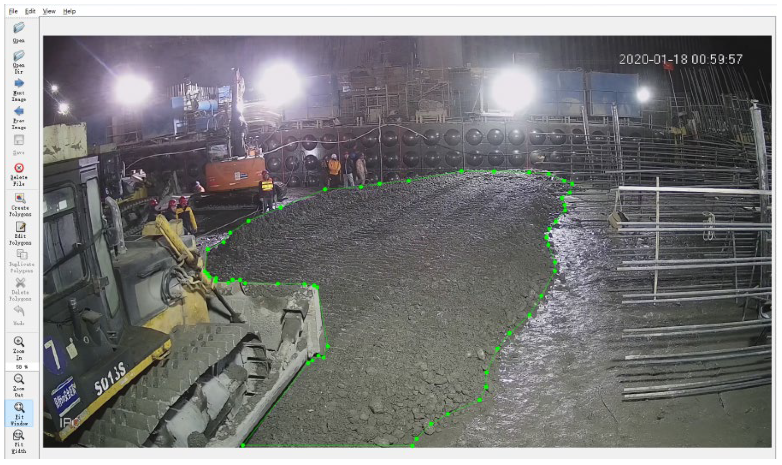
After annotating the extracted representative images, the annotation file and the generated mask for each image are shown in Figure 3.

Figure 3. Annotation Generation for Segmentation Mask Schematic.

To ensure the consistency and reliability of the annotation labels, all image annotation tasks were jointly performed by two researchers involved in this study, who first established a unified written annotation protocol. Upon completion, another researcher conducted random sampling inspections (approximately 20% of the total samples) and facilitated discussions to resolve any ambiguous boundaries or category judgments, with revisions made until a consensus was reached. This process minimized subjective variations to the greatest extent. Although this study did not conduct large-scale multi-annotator consistency statistics, the outstanding performance of the final model on an independent validation set indirectly confirms the validity and consistency of the annotation labels.

2.2. Monolith Recognition Model Training

This study employs two distinct semantic segmentation models to train the constructed dataset. The segmentation performance of each model under different quality conditions is compared to select the more suitable neural network for subsequent placement progress recognition in monolith scenarios.

2.2.1. DeepLab V3+ Semantic Segmentation Model

DeepLabv3+ is a classical semantic segmentation model whose core objective is to classify each pixel in an image, achieving pixel-level semantic understanding. Its core architecture is based on improved atrous convolution and an Atrous Spatial Pyramid Pooling (ASPP) module. The network backbone typically utilizes ResNet, where replacing traditional downsampling operations with atrous convolution in the final layers effectively preserves feature map resolution and expands the receptive field [15]. The ASPP module employs parallel atrous convolutions with different dilation rates and global average pooling, combined with 1 × 1 convolution and batch normalization (BN), to capture multi-scale contextual information [16]. Finally, feature concatenation and 1 × 1 convolution for dimensionality reduction are applied to generate high-level semantic features.

In this study, the DeepLabV3+ model employs ResNet-50, pre-trained on the ImageNet dataset, as its backbone feature extraction network. Appropriate training parameters were set to balance training effectiveness and speed, including the learning rate, decay factor, learning rate scheduling strategy, number of training epochs, and whether to freeze layers. Given the use of an NVIDIA GeForce RTX 3080 Ti GPU (NVIDIA Corporation; Santa Clara, CA, USA) and images resized to 1300 × 750 pixels, and considering established practices in semantic segmentation training, the learning rate was set to 7 × 10⁻⁴, weight decay to 1× 10⁻⁴ (to prevent overfitting), the Adam optimizer was used for learning rate scheduling, the total number of training epochs was 100, the batch size was 16, and no frozen training was applied (fine-tuning the model to reduce GPU memory pressure during training).

The annotated images and their corresponding masks were organized into the training directory to initiate the training process. The curves for training Loss and IoU during training are shown in Figure 4.

Figure 4. DeepLabV3+ Training Process: Total Loss (Left) and IoU (Right).

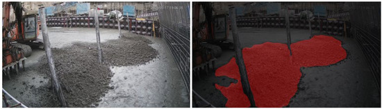
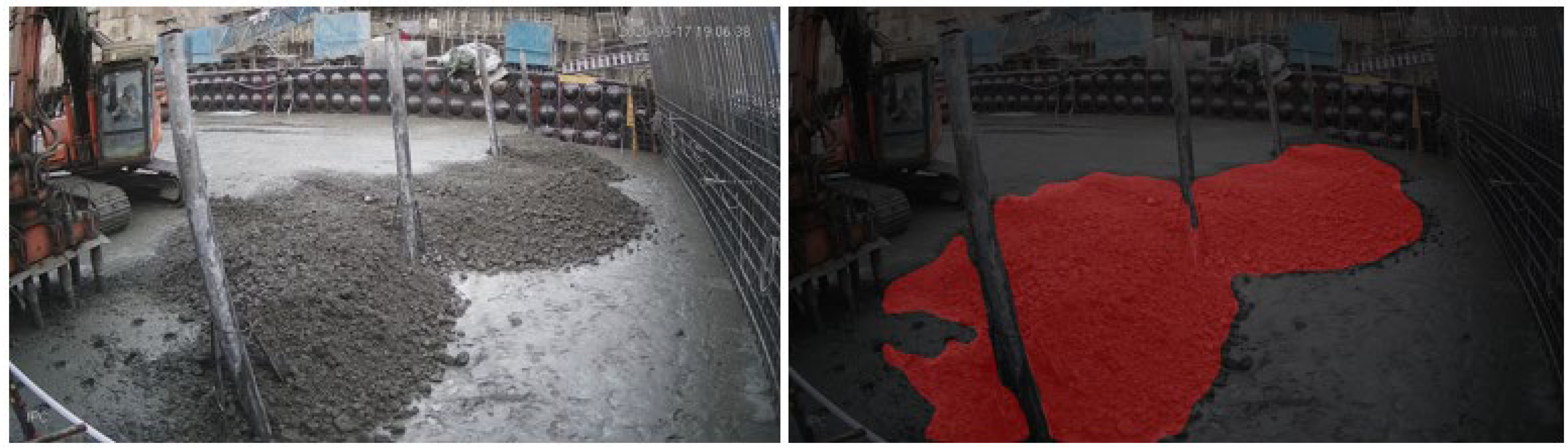
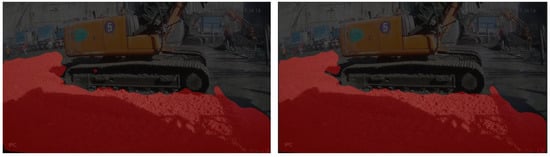
It can be observed that the model ceased significant reduction in Loss and improvement in IoU around epoch 100, indicating that optimal training accuracy was achieved at this point with a low overfitting rate. The model from this epoch was selected as the optimal DeepLab V3+ model. Its recognition performance for vibrated concrete is demonstrated in Figure 5.

Figure 5. DeepLabV3+ Recognition Result.

2.2.2. U-Net Semantic Segmentation Model

The U-Net semantic segmentation model also demonstrates excellent performance in numerous scenarios. U-Net employs a unique symmetric U-shaped architecture, consisting of an encoder (contracting path) on the left and a decoder (expanding path) on the right. The encoder extracts image features and reduces spatial dimensions through multiple layers of convolution and pooling, capturing global contextual information. The decoder gradually restores image resolution via transposed convolution (up-sampling) [20], and at each level, it incorporates feature maps from the corresponding encoder layer through skip connections [21]. This fusion of shallow detail and deep semantics enables precise target localization. The final pixel-level segmentation result is generated through a convolutional output layer.

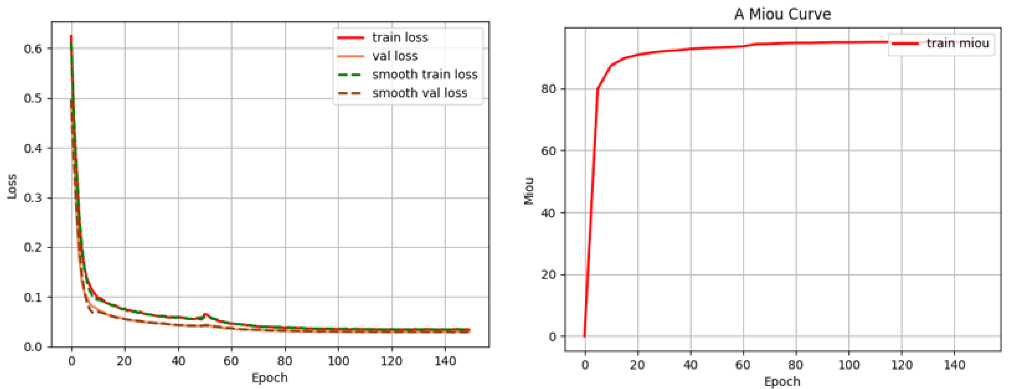
Adapted to the U-Net architecture, the learning rate was set to 5 × 10⁻⁴, weight decay to 1 × 10⁻⁴, the Adam optimizer was used, the total number of training epochs was 50, the batch size was 16, and no frozen training was applied.

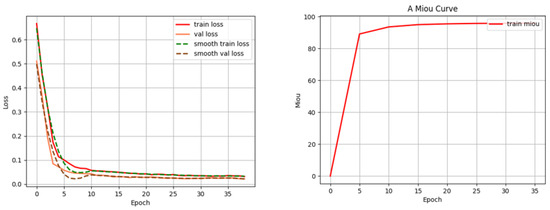
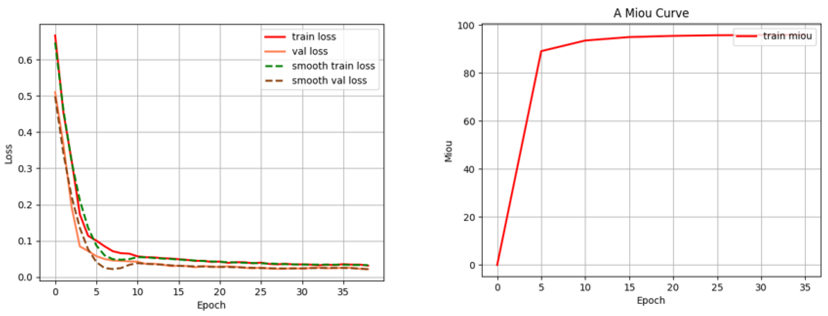
The annotated images and their corresponding masks were organized into the training directory to initiate the training process. The curves for training Loss and IoU during training are shown in Figure 6.

Figure 6. U-Net Training Process: Total Loss (Left) and IoU (Right).

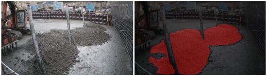
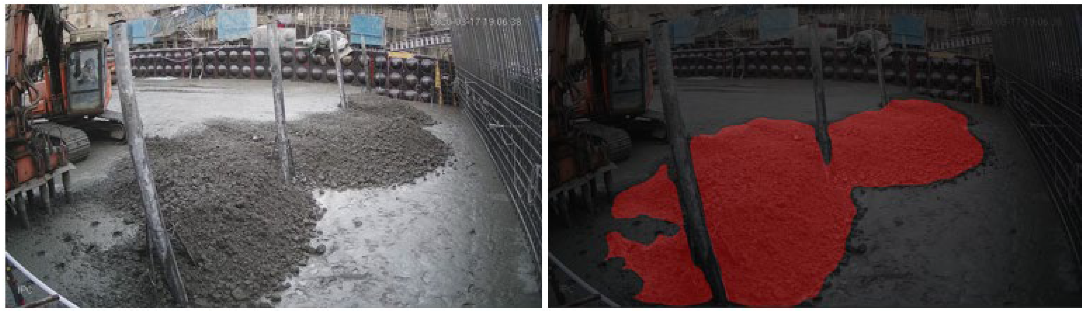
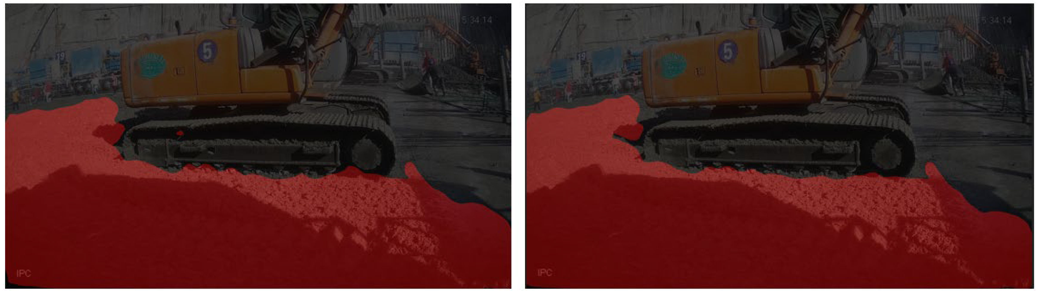
It can be observed that the U-Net model converged very rapidly, ceasing significant reduction in Loss and improvement in IoU around epoch 30, indicating that optimal training accuracy was achieved at this point with a low overfitting rate. The model from this epoch was selected as the optimal U-Net model. Its recognition performance for vibrated concrete is demonstrated in Figure 7.

Figure 7. U-Net Recognition Result.

2.3. Image Enhancement Module

2.3.1. Introduction to Dehazing Algorithms

Dehazing is often performed concurrently with luminance normalization. Generally, dehazing algorithms incorporate an image enhancement component for brightness balancing. Image enhancement techniques for hazy images can be broadly categorized into two types: prior-based methods and learning-based methods, each described below.

(1)

Prior-based Methods

Traditional prior-based methods rely on predefined assumptions about haze occurrence and distribution patterns, utilizing inherent image characteristics and physical laws to perform dehazing and enhancement through fixed algorithms. Common algorithms include Retinex, Dark Channel Prior (DCP), and image filtering. However, the effectiveness of prior-based methods depends heavily on the validity of the prior, and they often exhibit poor robustness in complex scenes.

The Retinex algorithm is expressed by Equation (1), where R represents the reflectance component (object properties), and L denotes the illumination component. Together, they form the image S. Traditional Retinex algorithms enhance images by separately processing the RGB channels, but this often leads to color distortion and halo artifacts. Consequently, improved Retinex algorithms incorporating color correction and parameter optimization have largely superseded the traditional approach [22].

$$S\left(x,y\right)=R(x,y)\times L(x,y)$$

(1)

The Dark Channel Prior is an image enhancement algorithm that approximates atmospheric conditions from image information to achieve dehazing. Its mathematical expression is given by Equation (2), where J is the clear image, Ω(x) is a local patch around pixel *x*, and J^dark is the derived dark channel. Combined with the atmospheric scattering model (Equation (3)), where I(x) is the observed hazy image, t(x) is the transmission map, and A is the atmospheric light, the clear image J(x) can be recovered by estimating t(x) and A from the hazy image [23].

$$J^{dark}\left(x\right)=\underset{c\in \left\{RGB\right\}}{min}(\underset{y\in \Omega \left(x\right)}{min}{J}^c\left(y\right))\approx 0$$

(2)

$$I\left(x\right)=J\left(x\right)t\left(x\right)+A(1-t\left(x\right))$$

(3)

Image filtering methods remove noise in the probabilistic domain by applying various filters, such as Gaussian filters, bilateral filters [24], and guided filters [25]. These methods are increasingly being integrated with deep learning techniques, yielding improved results.

(2)

Learning-based Methods

Learning-based methods train neural networks to learn a mapping from hazy to haze-free images. They often employ CNN or other deep learning models [26] in an end-to-end manner to generate clear images directly [27,28,29]. These approaches do not rely on physical models but require large amounts of paired data for training. Limited data leads to inferior dehazing performance and poor generalization, and these methods often lack interpretability [30].

2.3.2. Image Dehazing and Enhancement

Both aforementioned categories have inherent limitations. Integrating them is key to improving dehazing algorithm performance. This study employs a two-stage method based on RefineDNet [31] for haze enhancement and luminance normalization. In the first stage, the dark channel prior method is used to preliminarily restore image visibility, while potentially preserving artifacts it may introduce. In the second stage, a refining neural network optimizes both the initially processed image and the estimated transmission map. Image quality assessment metrics are used to quantify the enhancement weight for different regions, ultimately producing an enhanced output that more closely resembles a natural image.

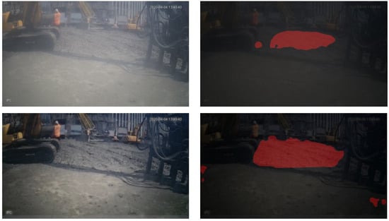
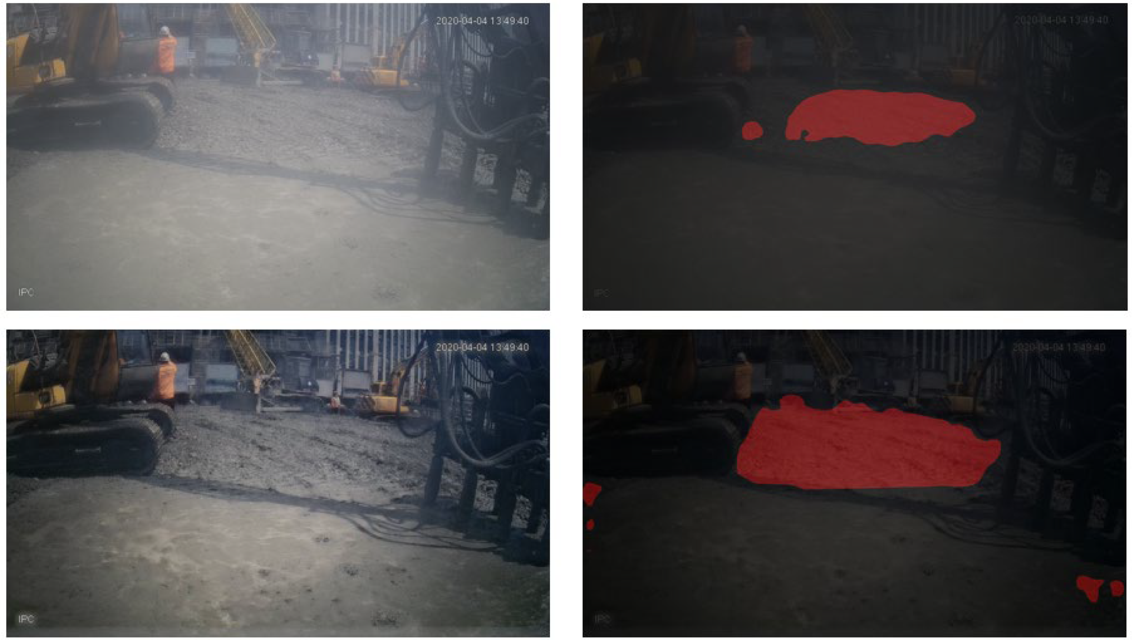
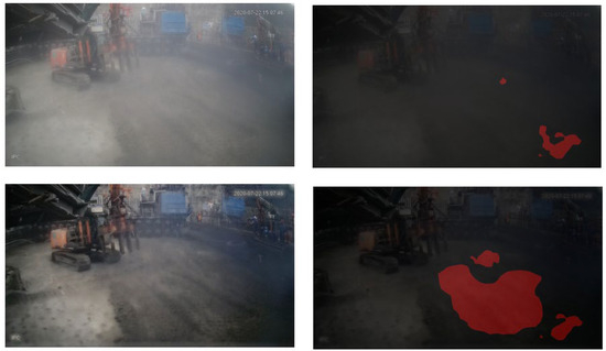
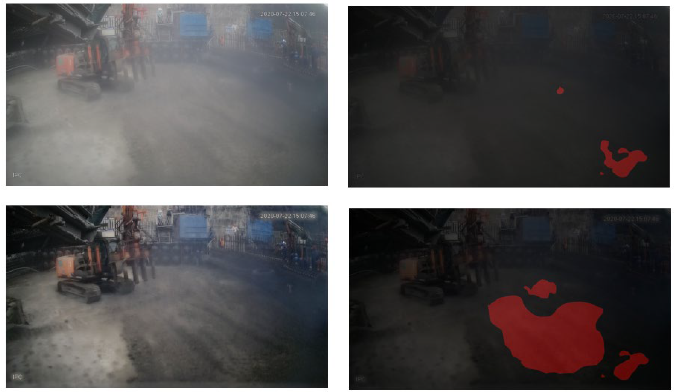
Based on the severity of haze or lens contamination, the haze dataset can be further divided into dense haze and light haze categories. Although both share similar characteristics, the dataset for dense haze is relatively small. Therefore, this study does not stratify the haze dataset, although the concrete segmentation model’s performance varies significantly under these two levels of interference. The segmentation effects on images affected by varying degrees of haze, before and after dehazing processing, are shown in Figure 8 and Figure 9.

Figure 8. Image Segmentation Comparison Before (Top) and After (Bottom) Enhancement for Light Haze.

Figure 9. Image Segmentation Comparison Before (Top) and After (Bottom) Enhancement for Dense Haze.

After enhancement for light haze, the concrete segmentation accuracy improved significantly, with boundaries becoming clearly identifiable and segmentation precise. However, in dense haze scenarios, where excessive information is lost, image details cannot be fully recovered post-enhancement. Consequently, the performance of the concrete segmentation model remains suboptimal, albeit improved overall. A comparison of model performance before and after dehazing is presented in Table 2. The results show an IoU increase of 20.1% and a precision increase of 17.5%, indicating that the dehazing process significantly enhances the accuracy of the concrete segmentation model.

Table 2. Model Performance Comparison Before and After Processing.

Metric	IoU	Precision
With Haze Effects	64.3%	68.2%
After Dehazing and Luminance Normalization	81.4%	82.7%

2.4. All-Cycle Monolith Placement Progress Analysis Method

2.4.1. Filtering Scheme

This study developed a method for analyzing concrete placement progress throughout the entire construction cycle. First, an improved U-Net semantic segmentation model is used to perform high-precision segmentation of construction images, achieving pixel-level distinction between vibrated and non-vibrated concrete. Based on the real-time segmentation results, the proportional area (pixel ratio) of each concrete type and its changes are calculated to identify the construction status, track construction events, and accurately determine the placement progress.

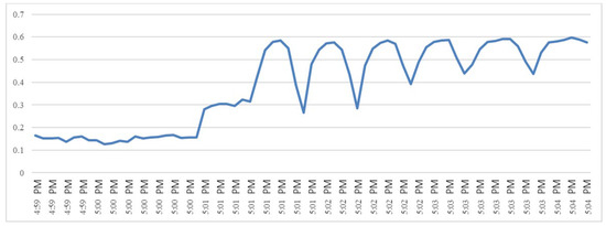
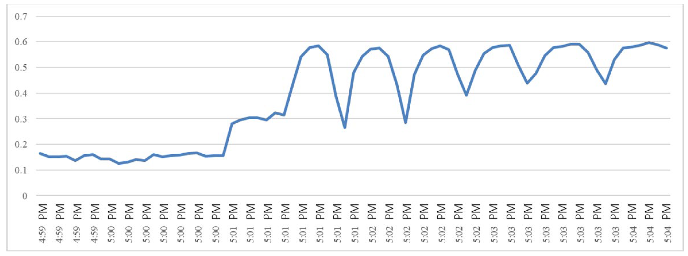
Due to obstructions and limitations in model segmentation accuracy, the concrete trend graph is affected by noise, particularly low-frequency noise, manifesting as local value oscillations, as shown in Figure 10. The repeated movement of construction machinery through the field of view, occluding non-vibrated concrete, causes local troughs in its area proportion. To mitigate this effect while preserving the underlying trend of the curve, a filtering method is applied to process the concrete change time series.

Figure 10. Variation in Non-Vibrated Concrete Proportion under Noise Influence.

Commonly used filtering methods for time series can be broadly categorized into three types. Classical linear filters use simple functions for linear data combinations (e.g., weighted sums) and achieve filtering directly through frequency domain design (e.g., low-pass, high-pass). Classic algorithms like moving average and exponential smoothing are simple in form and easy to implement. Nonlinear filters involve a nonlinear relationship between input and output, utilizing operations like ranking or conditional checks. They are less sensitive to outliers and impulse noise. Classic algorithms like median filtering and Kalman filtering can handle non-Gaussian noise and are suitable for nonlinear systems. Adaptive filters update their coefficients in real-time based on the input signal, automatically adapting to unknown or time-varying noise characteristics without prior knowledge. Classic algorithms include Least Mean Squares (LMS) and Recursive Least Squares (RLS) filters, which are suited for non-stationary signals like time-varying channels or burst noise. Furthermore, current research focuses on using deep learning models such as LSTMs and CNNs to dynamically learn the mapping between noise and signal, handling complex nonlinear noise and performing well on high-dimensional time series [32,33,34].

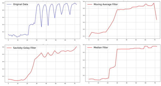
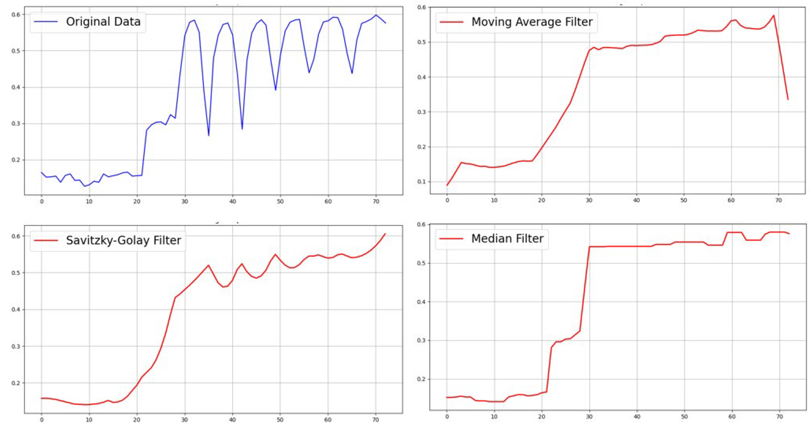
As the time series in this study contains numerous significant outliers and only the data trend needs to be preserved, three methods were applied and compared: moving average filter, Savitzky–Golay filter [35], and median filter. The filtering effects are shown in Figure 11. The moving average filter noticeably reduces noise; however, since the outliers are small values, the filtered data are biased low compared to normal values, damaging valid information. The Savitzky–Golay filter is powerful for preserving signal features, effectively retaining the change trend while smoothing the curve, but it performs poorly in correcting outliers. The median filter effectively removes the impulse noise in this time series while preserving the original trend, achieving the best balance between noise suppression and feature preservation.

Figure 11. Original Sequence (Top Left), Moving Average (Top Right), Savitzky–Golay Filter (Bottom Left), and Median Filter (Bottom Right).

2.4.2. Construction Status Analysis Method

Based on field construction experience and the changing trend of the non-vibrated concrete area, the construction status is classified into three mutually exclusive types: spreading status, vibration status, and stagnation status. These three statuses constitute the basic scenarios of monolith construction and typically occur sequentially during the placement process. Therefore, accurately analyzing the construction status is a prerequisite for determining placement progress and subsequently evaluating construction quality.

To ensure accurate trend judgment, the data is discretely differentiated and ternary encoded: derivative values greater than 0.002 are assigned a value of 1, values less than −0.002 are assigned −1, and others are 0. This threshold can be adjusted within the range [0.001, 0.003] depending on the situation. The result is shown in Figure 12.

Figure 12. Non-Vibrated Concrete Proportion and Construction Status Variation.

The spreading status is represented in the concrete proportion graph by a continuous increase in the non-vibrated concrete proportion and a decrease in the vibrated concrete proportion, corresponding to a derivative value of 1. The vibration status is represented by a continuous decrease in the non-vibrated concrete proportion and an increase in the vibrated concrete proportion, corresponding to a derivative value of −1. All other cases are classified as stagnation status.

Since spreading and vibration are not performed continuously over time but rather intermittently—manifesting as intermittent spreading or vibration during construction—the derivative graph contains numerous noise-like fluctuations. However, these short stagnation periods can still be considered part of the spreading or vibration phase. Therefore, adjacent statuses are merged using a filtering-like approach: for each time point, 10 preceding and succeeding points are sampled. If the proportion of points identified as spreading or vibration exceeds 40%, the current point is assigned to the corresponding status; otherwise, it is deemed a stagnation point. The processed construction status determination is shown in Figure 13.

Figure 13. Processed Non-Vibrated Concrete Proportion and Construction Status Variation.

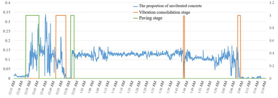
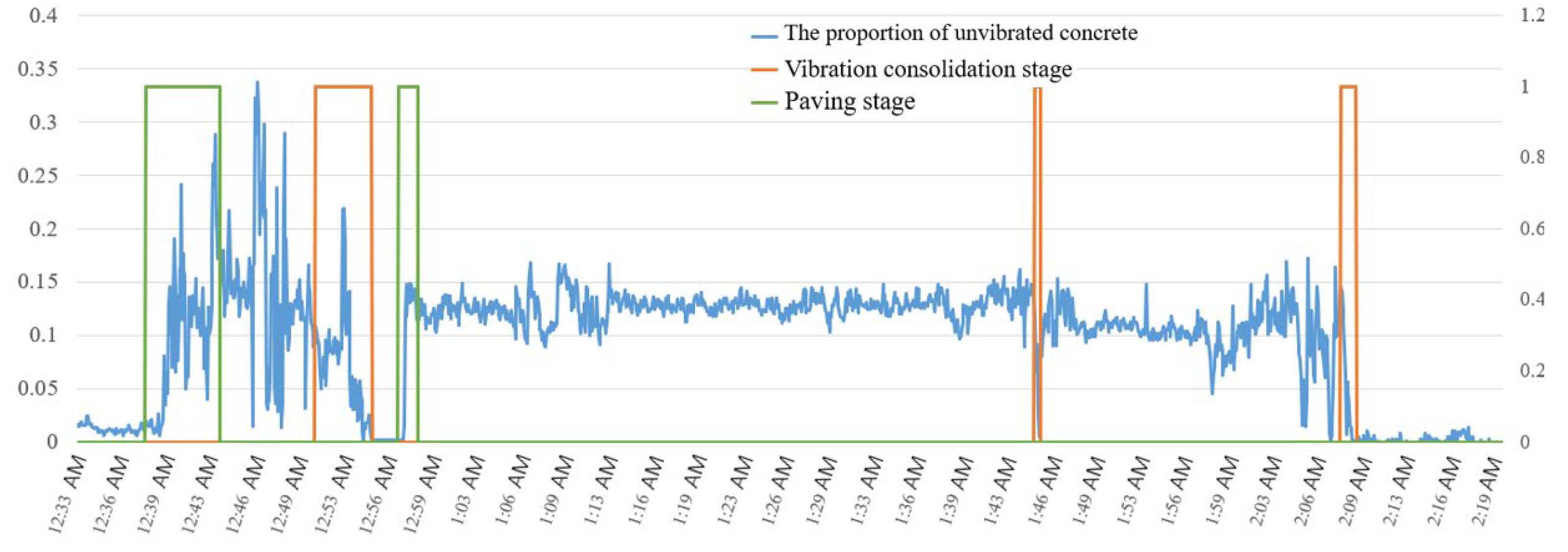
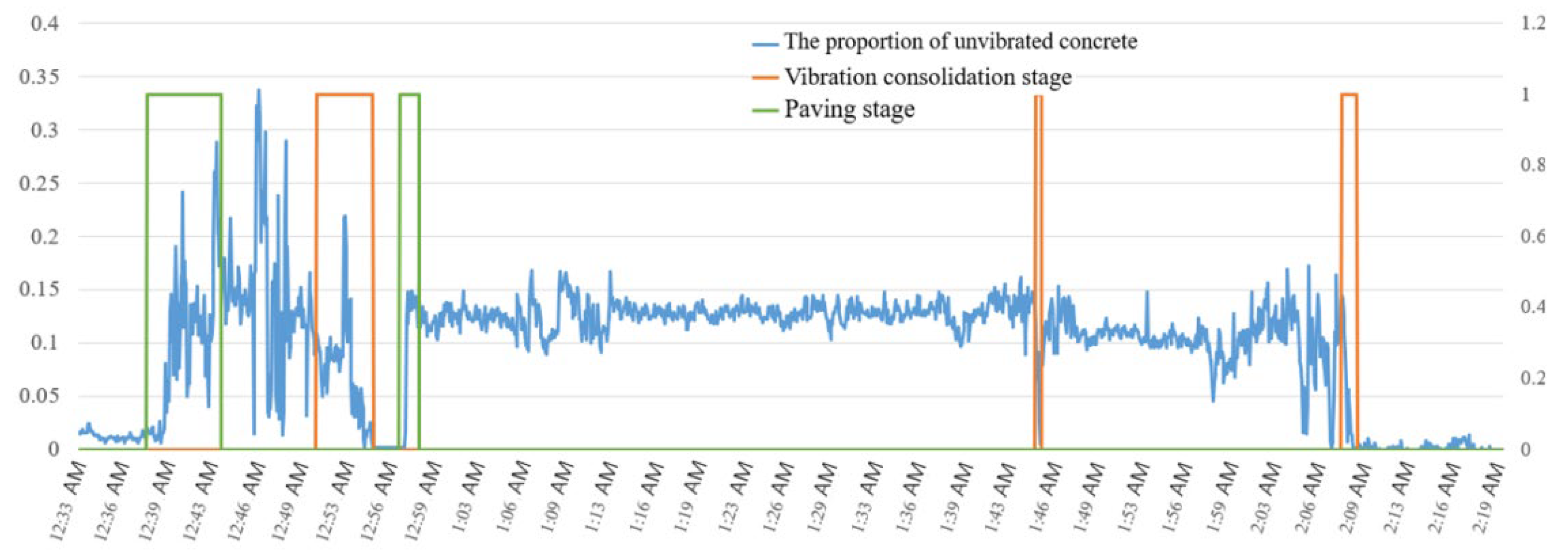
According to the onsite construction video, the scenario underwent two spreading phases and two vibration phases. The durations of the two spreading phases were from 12:39 to 12:42 and from 12:57 to 12:59, respectively. The durations of the two vibration phases were from 12:46 to 12:54 and from 14:04 to 14:08, respectively. These timings are largely consistent with the status graph segmentation results, indicating the accuracy of the proposed method for identifying spreading and vibration phases.

3. Case Study

3.1. Model Performance

3.1.1. Model Training and Inference Efficiency Comparison

The training and inference efficiency of the two models were compared using two approaches. First, a comparison of their basic performance was conducted, as shown in Table 3, focusing on the number of parameters, average inference time per image, training time per epoch, and IoU performance on the training set. The average inference time per image refers to the total time required to input a single image, load the model, perform segmentation, and release memory. The training set IoU represents the model’s recognition accuracy on the entire dataset. In this task, U-Net demonstrated its lightweight advantage. With a smaller number of parameters, it maintained comparable recognition accuracy while achieving an average inference time approximately 27% faster than DeepLabV3+. This indicates that U-Net can achieve good efficiency with lower hardware requirements. Regarding training time, U-Net was about 36% faster per epoch than DeepLabV3+ and required fewer epochs to reach the optimal model. DeepLabV3+ maintained its precise and professional style suitable for complex scenes; however, for this study, its inference efficiency was inferior to the U-Net architecture.

Table 3. Basic Model Performance.

Metric	U-Net	DeepLabV3+
Number of Parameters	28 M	47 M
Avg. Inference Time/Image	3.8 s	5.2 s
Training Time per Epoch	30.8 s	48.8 s
Training Set IoU	87.6%	88.7%

Furthermore, both models were used to sequentially process over 1600 images from the dataset in a single run. Additionally, a 2 h construction site video was processed, extracting one image every 250 frames (10 s) for segmentation. The performance is summarized in Table 4. The total processing time for the dataset includes reading the input directory, loading the model, sequential segmentation, and releasing memory. The average frame rate refers to the average number of video frames processed per second (including frame extraction). The U-Net model outperformed the DeepLabV3+ model across all three metrics, highlighting its advantage.

Table 4. Model Framerate Performance.

Metric	U-Net	DeepLabV3+
Total Dataset Process Time	48.21 s	60.12 s
Total Video Process Time	59.74 s	75.32 s
Average Frame Rate	28	22

3.1.2. Segmentation Accuracy Comparison on High-Quality Images

The performance of both models on high-quality images is shown in Figure 14. Both models maintained high accuracy on high-quality images. The aggregated metrics from processing each image in the dataset are presented in Table 5. Evidently, on high-quality image data, the performance of the two models was very similar. Particularly for the core metrics IoU and Precision, the U-Net network achieved accuracy on par with DeepLabV3+. This indicates that using U-Net has minimal impact on segmentation accuracy for these images, maintaining high segmentation performance.

Figure 14. High-Quality Image Recognition (Left: DeepLabV3+, Right: U-Net).

Table 5. Model Performance on High-Quality Dataset.

Metric	U-Net	DeepLabV3+
IoU	91.9%	92.1%
F1-Score	88.6%	89.7%
Precision	92.2%	92.0%

3.1.3. Segmentation Accuracy Comparison on Low-Quality Images

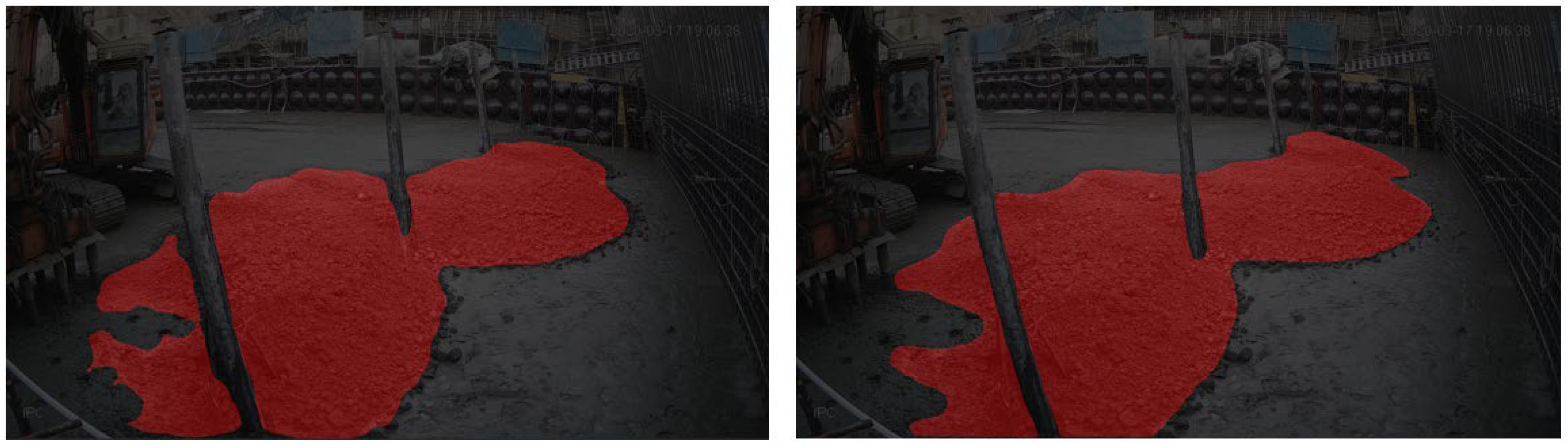
The performance of both models on low-quality images is shown in Figure 15. In low-light images affected by glare, the segmentation effectiveness of both models was significantly impacted, with a substantial decrease in the ability to segment the correct class, though the impact on background class segmentation was less pronounced. In low-quality images affected by occlusion, both models experienced a minor decline in performance, mainly manifesting as less distinct boundary segmentation and reduced ability to identify background classes. In low-light images affected by haze or poor lighting, the recognition ability for both the correct class and background classes decreased significantly, varying with the degree of haze influence.

Figure 15. Occluded Image Recognition (Left: DeepLabV3+, Right: U-Net).

The quantitative performance is shown in Table 6. Overall, U-Net performed slightly better across these challenging conditions.

Table 6. Performance on Low-Quality Images.

Metric	U-Net	DeepLabV3+
IoU (Glare Affected)	71.2%	74.3%
IoU (Occlusion Affected)	82.1%	81.3%
IoU (Haze Affected)	63.1%	69.6%
Precision (Glare Affected)	70.3%	74.1%
Precision (Occlusion Affected)	80.3%	81.0%
Precision (Haze Affected)	63.2%	68.7%

3.1.4. Overall Comparative Analysis

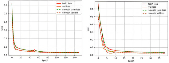
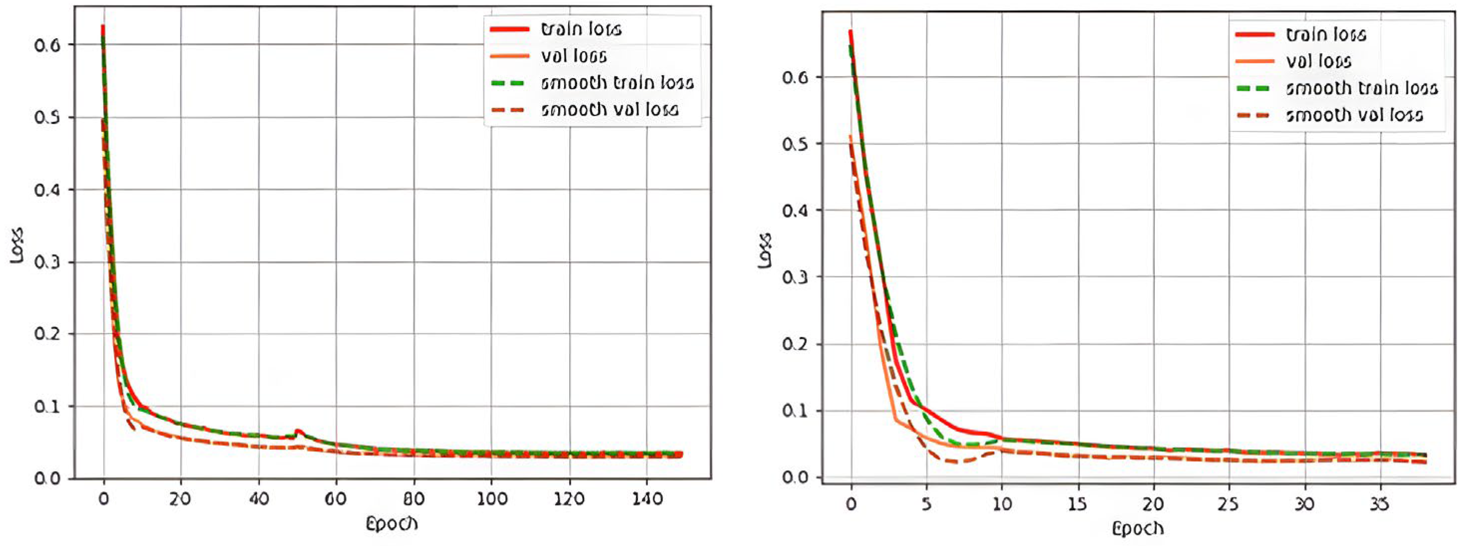
Two different semantic segmentation models were trained on the constructed dataset, and their segmentation performance was compared across different image qualities. The DeepLabV3+ model [3], based on improved atrous convolution and an atrous spatial pyramid pooling module, demonstrates high performance in numerous scenarios. The U-Net model [4], with its improved symmetric encoder–decoder structure, holds significant advantages in small-sample image segmentation tasks. The training loss curves for both models on the full dataset are shown in Figure 16.

Figure 16. Training Loss for DeepLab V3+ (Left) and U-Net (Right).

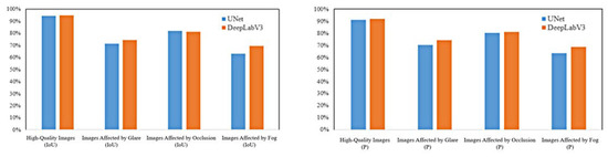
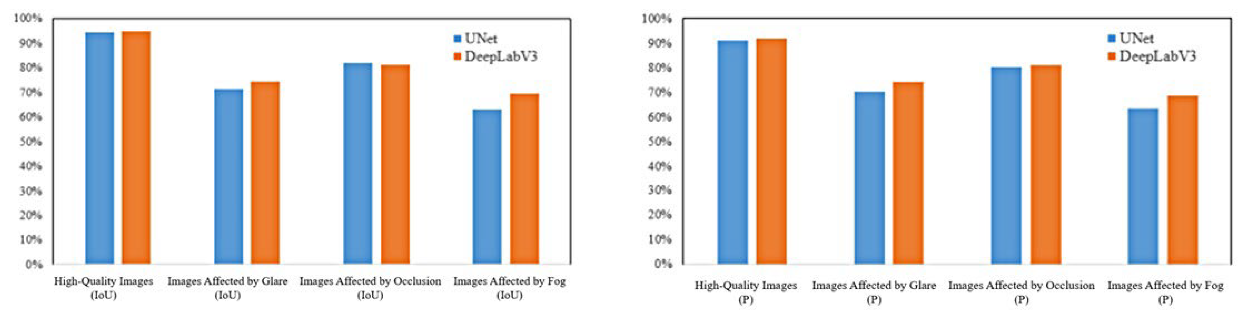
Compared to high recall (lower false negative rate), this study is more concerned with the model’s ability to completely segment every pixel belonging to concrete. Therefore, the Intersection over Union (IoU) is selected as the primary evaluation metric. The low-quality image dataset was subdivided into glare-affected, haze-affected, and occlusion-affected datasets. A comparison of the two models’ performance across these datasets is shown in Figure 17.

Figure 17. Performance Comparison of the Two Models on Different Datasets.

Both models performed well on high-quality images. For low-quality images: under glare-affected low-light conditions, both models experienced a significant drop in the ability to segment the correct class; under occlusion-affected conditions, boundary segmentation became less distinct, and background recognition ability decreased; under haze-affected low-light conditions, the segmentation accuracy of both models was adversely affected. Furthermore, in continuous video stream segmentation, the DeepLabV3+ model achieved a frame rate of 22 fps, whereas the U-Net model reached 28 fps. Consequently, considering all performance aspects—both speed and accuracy—the U-Net model was selected as the concrete segmentation model for this study.

The comparative experiments in this study aim to evaluate the adaptability and efficiency of two mainstream architectures under the same training strategy (with fixed hyperparameters) within this specific scenario. Although exhaustive hyperparameter tuning was not conducted for each model—which might have left some of DeepLabV3+’s accuracy potential unrealized—the experiments clearly elucidate the performance-efficiency trade-off between the two. As shown in Table 3, U-Net achieves segmentation accuracy comparable to DeepLabV3+ (with an IoU difference of less than 1%) while requiring fewer parameters and offering faster inference speed. Given the practical deployment requirements for real-time processing (>20 frames per second) and possible constraints of edge computing devices, U-Net provides a more favorable balance between accuracy and efficiency. Consequently, it was selected as the core model for subsequent progress analysis.

3.2. Placement Progress Segmentation Results

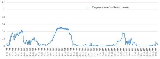
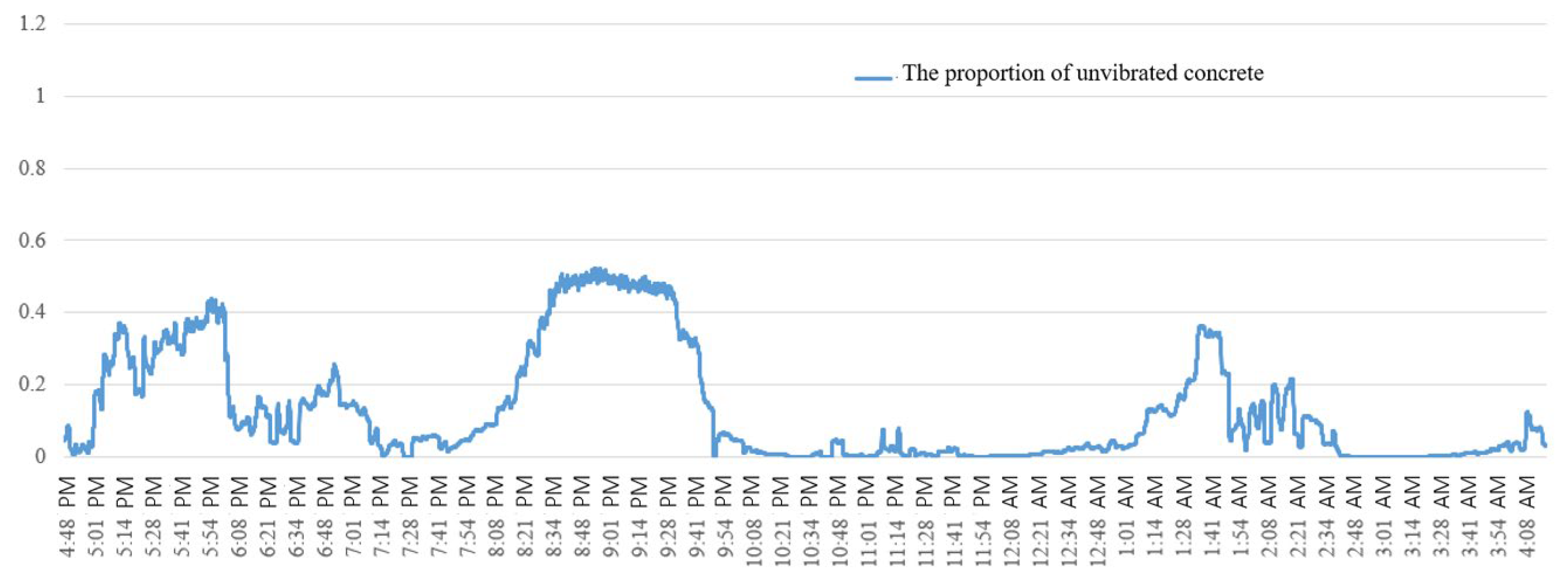
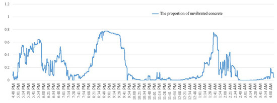
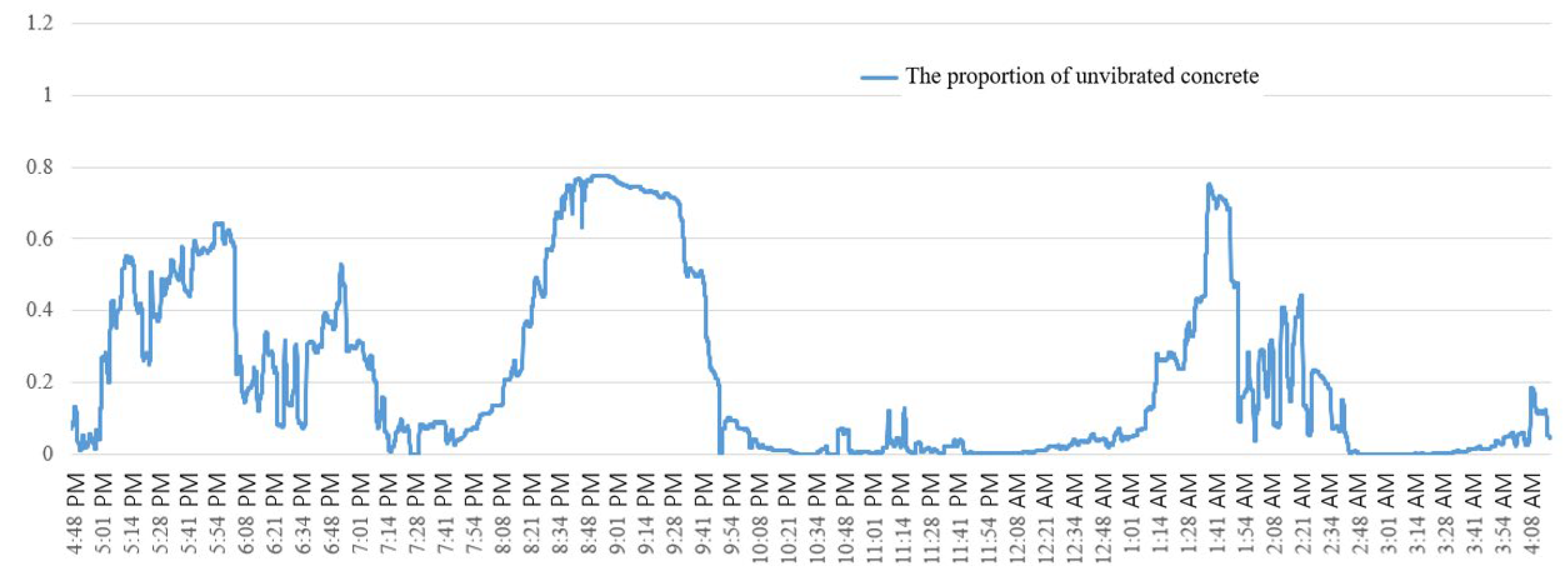
A 12 h continuous video of the placement process in Monolith No. 3 at the Baihetan project was selected for real-time analysis using the concrete segmentation-based method. One frame was extracted every 15 s for segmenting the non-vibrated concrete. For this case study, a one-dimensional median filter was applied to denoise the time series of the uncompacted concrete ratio. After multiple trials, the window size of the filter was set to 15 data points. This value was determined based on an analysis of the typical duration of onsite machinery occlusion and the data sampling interval, aiming to effectively suppress impulse noise caused by transient obstructions while preserving the sustained ratio variation trends resulting from actual spreading or vibration processes. After this filtering, the noise in the sequence was significantly reduced, providing a more stable input for subsequent derivative calculations and state judgment. The variation curve of the non-vibrated concrete proportion after filtering is shown in Figure 18.

Figure 18. Variation in Non-Vibrated Concrete Proportion.

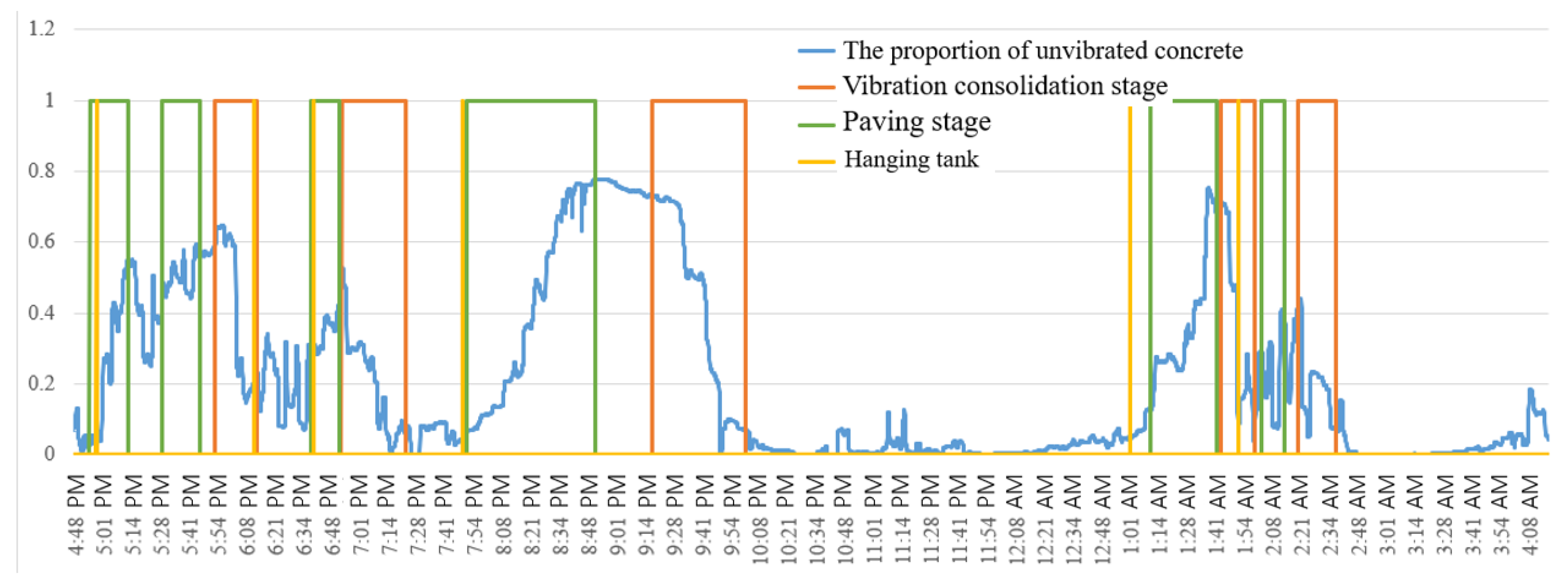
Based on the video footage, during the first three hours with good visibility, the concrete segmentation model achieved high accuracy, effectively capturing the trend of the non-vibrated concrete proportion, despite occasional local troughs caused by machinery occlusion. However, after nightfall, under low-light conditions—especially with the activation of high-intensity onsite lighting—the segmentation accuracy declined. While the general trend of non-vibrated concrete change was retained, the estimated proportion deviated significantly from the actual value. Furthermore, error increased markedly, and numerous outliers remained even after filtering. By integrating a hopper recognition method, the status was segmented as shown in Figure 19.

Figure 19. Construction Status Segmentation.

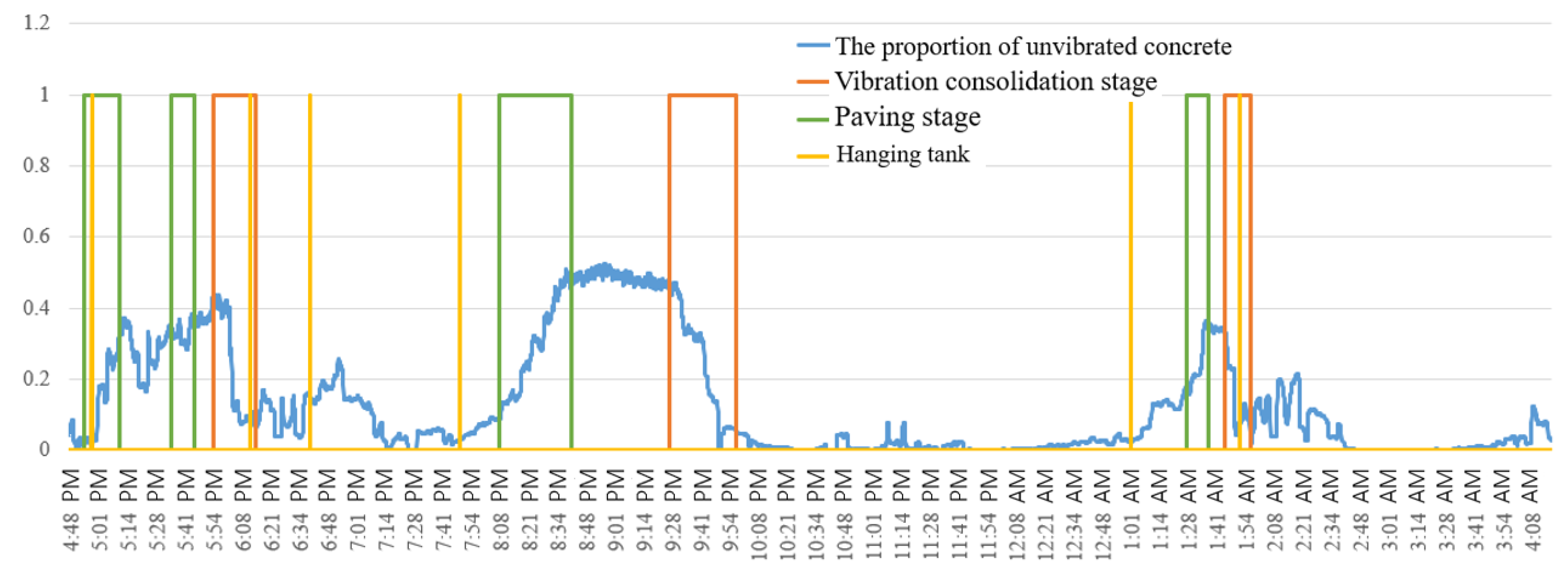
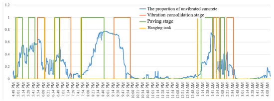
Throughout the placement process, the hopper appeared four times. Corroborated by the video, Monolith No. 3 underwent four spreading phases during the recording period. A comparison of the non-vibrated concrete proportion changes is shown in Figure 20. After applying three different image enhancement techniques, the recognition accuracy of concrete improved across all periods. Particularly after nightfall, the proportion of non-vibrated concrete was significantly higher, and its peaks were generally consistent compared to results without the image optimization module.

Figure 20. Non-Vibrated Concrete Proportion After Adding Image Optimization.

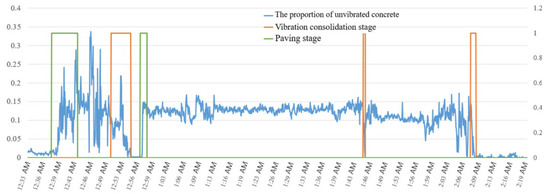
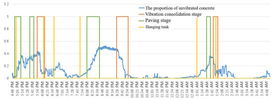
The status was segmented based on the variation in non-vibrated concrete proportion, and further refined with hopper recognition, as illustrated in Figure 21. According to the construction phase segmentation results, the recorded process included six spreading phases and five vibration phases. The first two spreading phases were originally part of one continuous phase but were segmented separately due to persistent interference from construction equipment, which hampered accurate proportion estimation.

Figure 21. Construction Status Segmentation After Adding Image Optimization.

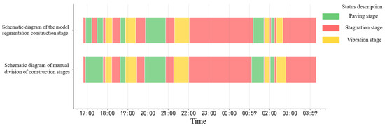
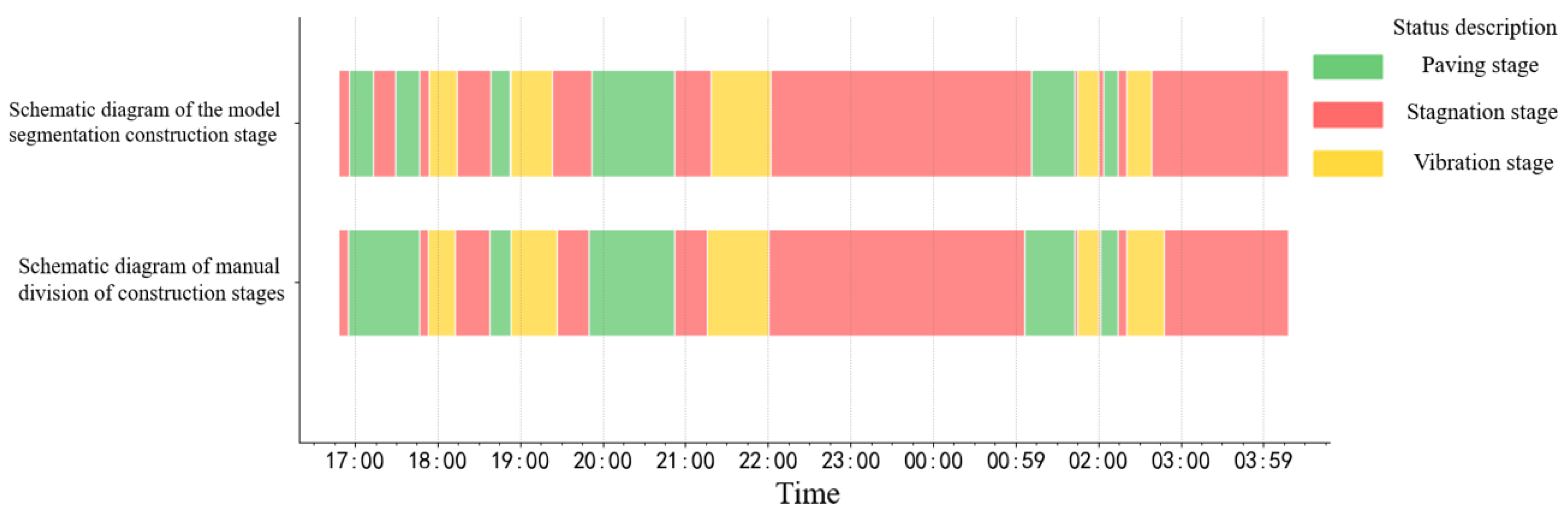
The construction phases were manually identified from the video and compared with the model segmentation results, as shown in the Gantt chart in Figure 22. The “8.2% segmentation error” mentioned in this paper refers to the temporal interval error in construction phase partitioning. The specific calculation method is as follows: for each construction phase (e.g., paving or vibration) identified in the video sequence, the absolute time difference between its model-determined start/end points and the manually annotated start/end points is calculated. The absolute time differences for all phases are summed, then divided by the total duration of the video. The result is finally expressed as a percentage. This error metric directly reflects the model’s accuracy in temporally tracking construction progress.

$$\mathrm{Error}={\displaystyle \frac{{\sum }_{i=1}^N\mid t_{\mathrm{model},\mathrm{start}}^i-t_{\mathrm{human},\mathrm{start}}^i\mid +\mid t_{\mathrm{model},\mathrm{end}}^i-t_{\mathrm{human},\mathrm{end}}^i\mid }{T_{\mathrm{total}}}}\times 100\mathrm{\%}$$

(4)

Figure 22. Gantt Chart Comparing Model-Segmented and Manually Segmented Construction Phases.

The model-based segmentation was largely accurate in identifying construction phases, aligning well with manual observations. Although minor discrepancies existed in the precise timing of phases, the overall error was only 8.2%. This strongly indicates that the proposed method can effectively replace manual monitoring for real-time identification of construction phases, thereby enabling real-time analysis of placement progress.

This chapter utilized a high-precision concrete segmentation model to generate a trend chart of the proportion of non-vibrated concrete. Three filtering algorithms were compared, and the median filter was ultimately selected to process the trend data. Based on this, a construction phase segmentation method was proposed, classifying the process into spreading, vibration, and stagnation phases. The spreading phase is characterized by a continuous increase in the proportion of non-vibrated concrete and a corresponding decrease in vibrated concrete, while the vibration phase exhibits the opposite trend. All other scenarios are classified as stagnation. Furthermore, the precise event of concrete unloading was incorporated by employing hopper detection to assist in segmenting the construction phases. The method was validated using a continuous placement process in Monolith No. 3 at the Baihetan project, where the model achieved a segmentation error of only 8.2% compared to manual segmentation. This result effectively demonstrates that the proposed method can serve as an intelligent, real-time replacement for manual monitoring in identifying construction events.

4. Conclusions

This study developed a deep learning-based method for identifying vibrated and non-vibrated concrete, establishing a semantic segmentation model for recognizing placement progress on construction faces. A high-precision dataset of various construction elements was created, consisting of 220 high-quality images, 93 occluded images, 43 haze-affected images, and 78 glare-affected images. The performance of the U-Net and DeepLabV3+ models was evaluated across different scenarios. While the DeepLabV3+ model offered higher accuracy, its inference speed was only 78% of that of the U-Net model. Consequently, the U-Net model, with an IoU of 89%, was selected as the concrete recognition model for subsequent analysis.

Based on this high-precision concrete segmentation model, a time series of the proportion of non-vibrated concrete was generated. The construction process was segmented into spreading, vibration, and stagnation phases by analyzing the characteristics of this curve. In a case study of continuous placement in Monolith No. 3 at the Baihetan project, the model achieved a mere 8.2% error compared to manual segmentation, confirming its real-time capability and reliability.

This research established a comprehensive real-time analysis framework for monitoring placement progress. However, several limitations and future research directions are identified:

(1)

Acquisition of Larger and More Detailed Datasets: Addressing the specificities of concrete construction scenarios requires integrating multi-source data to build a comprehensive, all-weather, multi-perspective, and finely detailed dataset. Emphasis should be placed on annotating images captured under extreme lighting and dynamic occlusion. Combining semi-automatic annotation tools with physics-based simulation engines to generate synthetic data can enhance sample diversity and annotation accuracy. Furthermore, establishing cross-construction site data sharing mechanisms—while ensuring privacy—would enable joint optimization using multi-site data, mitigating overfitting to single scenarios.

(2)

Model Lightweighting and Real-Time Optimization: Both the concrete segmentation model and auxiliary models (e.g., for image enhancement and hopper detection) are computationally intensive. Future work should explore adaptive model compression techniques and hardware acceleration solutions, such as employing knowledge distillation to transfer learning from complex models like YOLOv8 or U-Net to lightweight architectures. Developing a unified multi-task learning framework that integrates image segmentation, progress analysis, and anomaly detection into a single model could reduce redundant feature extraction, ultimately enabling low-power, real-time processing of long-sequence construction data.

(3)

Research Based on Construction Phases: This study extracted construction phases and segmented events solely from video, essentially using the camera as a sensor. Future work should focus on fusing data from other sensors to further assess construction quality and enable real-time supervision of placement progress.

(4)

Improving Transferability and Generalizability: The current dataset is limited to video from six monoliths at the Baihetan project. Construction scenes vary across different dams and project phases, and the imaging equipment used also affects picture quality. Therefore, enhancing model transferability and generalizability—making it applicable beyond specific projects or dam types—is crucial for broader adoption in diverse construction scenarios.

References

- Halder, S.; Afsari, K.; Serdakowski, J.; DeVito, S.; Ensafi, M.; Thabet, W. Real-Time and Remote Construction Progress Monitoring with a Quadruped Robot Using Augmented Reality. Buildings 2022, 12, 2027. [Google Scholar] [CrossRef] [Scilit]
- Ibrahimkhil, M.H.; Shen, X.; Barati, K.; Wang, C.C. Dynamic Progress Monitoring of Masonry Construction through Mobile SLAM Mapping and As-Built Modeling. Buildings 2023, 13, 930. [Google Scholar] [CrossRef] [Scilit]
- Song, W.; Guan, T.; Ren, B.; Yu, J.; Wang, J.; Wu, B. Real-Time Construction Simulation Coupling a Concrete Temperature Field Interval Prediction Model with Optimized Hybrid-Kernel RVM for Arch Dams. Energies 2020, 13, 4487. [Google Scholar] [CrossRef] [Scilit]
- Zhang, R.; Deng, R.; Zhang, Z.; Mao, Y. Vision-Based Real-Time Progress Tracking and Productivity Analysis of the Concrete Pouring Process. Dev. Built Environ. 2025, 21, 100609. [Google Scholar] [CrossRef] [Scilit]
- Wu, B.P.; Cui, B.; Ren, C.G.; Zhong, D.H. Research and Application of a Real-Time Monitoring System for Pouring and Rolling Construction Quality at Longkaikou RCC Dam. Water Resour. Hydropower Eng. 2013, 44, 62–65. [Google Scholar] [CrossRef]
- Gong, J.; Yu, Y.; Krishnamoorthy, R.; Roda, A. Real-Time Tracking of Concrete Vibration Effort for Intelligent Concrete Consolidation. Autom. Constr. 2015, 54, 12–24. [Google Scholar] [CrossRef] [Scilit]
- Tian, Z.; Bian, C. Visual Monitoring Method on Fresh Concrete Vibration. KSCE J. Civ. Eng. 2014, 18, 398–408. [Google Scholar] [CrossRef] [Scilit]
- Wang, R.; Zhong, D.H.; Wu, B.P.; Yue, P. Compaction Quality Assessment of Rockfill Dam Considering the Uncertainty of Material Sources under Real-Time Monitoring. J. Hydroelectr. Eng. 2015, 34, 146–152. [Google Scholar] [CrossRef]
- Guo, F.; Yang, J.; Liu, Z.; Tang, J. Haze Removal for Single Image: A Comprehensive Review. Neurocomputing 2023, 537, 85–109. [Google Scholar] [CrossRef] [Scilit]
- Hinton, G.E.; Osindero, S.; Teh, Y.-W. A Fast Learning Algorithm for Deep Belief Nets. Neural Comput. 2006, 18, 1527–1554. [Google Scholar] [CrossRef] [Scilit]
- Hong, K.; Wang, H.; Yuan, B.; Wang, T. Multiple Defects Inspection of Dam Spillway Surface Using Deep Learning and 3D Reconstruction Techniques. Buildings 2023, 13, 285. [Google Scholar] [CrossRef] [Scilit]
- Cuypers, S.; Bassier, M.; Vergauwen, M. Deep Learning on Construction Sites: A Case Study of Sparse Data Learning Techniques for Rebar Segmentation. Sensors 2021, 21, 5428. [Google Scholar] [CrossRef] [Scilit] [PubMed]
- Long, J.; Shelhamer, E.; Darrell, T. Fully Convolutional Networks for Semantic Segmentation. In Proceedings of the IEEE Conference on Computer Vision and Pattern Recognition, Boston, MA, USA, 7–12 June 2015; pp. 3431–3440. [Google Scholar]
- Chen, L.-C.; Papandreou, G.; Kokkinos, I.; Murphy, K.; Yuille, A.L. DeepLab: Semantic Image Segmentation with Deep Convolutional Nets, Atrous Convolution, and Fully Connected CRFs. IEEE Trans. Pattern Anal. Mach. Intell. 2018, 40, 834–848. [Google Scholar] [CrossRef] [Scilit] [PubMed]
- Chen, L.-C.; Zhu, Y.; Papandreou, G.; Schroff, F.; Adam, H. Encoder-Decoder with Atrous Separable Convolution for Semantic Image Segmentation. In Proceedings of the Computer Vision—ECCV 2018, Munich, Germany, 8–14 September 2018; Ferrari, V., Hebert, M., Sminchisescu, C., Weiss, Y., Eds.; Springer International Publishing: Cham, Switzerland, 2018; pp. 833–851. [Google Scholar]
- Chen, L.-C.; Papandreou, G.; Schroff, F.; Adam, H. Rethinking Atrous Convolution for Semantic Image Segmentation. arXiv 2017, arXiv:1706.05587. [Google Scholar] [CrossRef] [Scilit]
- Yann, L.; Bottou, L.; Bengio, Y. Gradient-Based Learning Applied to Document Recognition. Gradient-Based Learn. Appiled Doc. Recognit. 2002, 86, 2278–2324. [Google Scholar]
- Zhang, J.; Zhang, J. An Improved Nondestructive Semantic Segmentation Method for Concrete Dam Surface Crack Images with High Resolution. Math. Probl. Eng. 2020, 2020, 5054740. [Google Scholar] [CrossRef] [Scilit]
- Badrinarayanan, V.; Kendall, A.; Cipolla, R. SegNet: A Deep Convolutional Encoder-Decoder Architecture for Image Segmentation. IEEE Trans. Pattern Anal. Mach. Intell. 2017, 39, 2481–2495. [Google Scholar] [CrossRef] [Scilit]
- Jobson, D.J.; Rahman, Z.; Woodell, G.A. A Multiscale Retinex for Bridging the Gap between Color Images and the Human Observation of Scenes. IEEE Trans. Image Process. 1997, 6, 965–976. [Google Scholar] [CrossRef] [Scilit]
- Ronneberger, O.; Fischer, P.; Brox, T. U-Net: Convolutional Networks for Biomedical Image Segmentation. arXiv 2015, arXiv:1505.04597. [Google Scholar] [CrossRef] [Scilit]
- Land, E.H. The Retinex Theory of Color Vision. Sci. Am. 1977, 237, 108–129. [Google Scholar] [CrossRef] [Scilit]
- He, K.; Sun, J.; Tang, X. Single Image Haze Removal Using Dark Channel Prior. In Proceedings of the 2009 IEEE Conference on Computer Vision and Pattern Recognition, Miami, FL, USA, 20–25 June 2009; pp. 1956–1963. [Google Scholar]
- Aurich, V.; Weule, J. Non-Linear Gaussian Filters Performing Edge Preserving Diffusion. In Proceedings of the Mustererkennung 1995, Bielefeld, Germany, 13–15 September 1995; Sagerer, G., Posch, S., Kummert, F., Eds.; Springer: Berlin/Heidelberg, Germany, 1995; pp. 538–545. [Google Scholar]
- He, K.; Sun, J.; Tang, X. Guided Image Filtering. IEEE Trans. Pattern Anal. Mach. Intell. 2013, 35, 1397–1409. [Google Scholar] [CrossRef] [Scilit]
- Hu, H.; Zhang, C.; Luo, Y.; Wang, Y.; Han, J.; Ding, E. WordSup: Exploiting Word Annotations for Character Based Text Detection. In Proceedings of the 2017 IEEE International Conference on Computer Vision (ICCV), Venice, Italy, 22–29 October 2017; pp. 4950–4959. [Google Scholar]
- Suárez, P.L.; Sappa, A.D.; Vintimilla, B.X.; Hammoud, R.I. Deep Learning Based Single Image Dehazing. In Proceedings of the 2018 IEEE/CVF Conference on Computer Vision and Pattern Recognition Workshops (CVPRW), Salt Lake City, UT, USA, 18–22 June 2018; pp. 1250–12507. [Google Scholar]
- Choudhary, R.R.; Jisnu, K.K.; Meena, G. Image DeHazing Using Deep Learning Techniques. Procedia Comput. Sci. 2020, 167, 1110–1119. [Google Scholar] [CrossRef] [Scilit]
- Gui, J.; Cong, X.; Cao, Y.; Ren, W.; Zhang, J.; Zhang, J.; Tao, D. A Comprehensive Survey on Image Dehazing Based on Deep Learning. In Proceedings of the Thirtieth International Joint Conference on Artificial Intelligence, Montreal, QC, Canada, 19–26 August 2021; pp. 4426–4433. [Google Scholar]
- Ren, W.; Liu, S.; Zhang, H.; Pan, J.; Cao, X.; Yang, M.-H. Single Image Dehazing via Multi-Scale Convolutional Neural Networks. In Proceedings of the Computer Vision—ECCV 2016, Amsterdam, The Netherlands, 11–14 October 2016; Leibe, B., Matas, J., Sebe, N., Welling, M., Eds.; Springer International Publishing: Cham, Switzerland, 2016; pp. 154–169. [Google Scholar]
- Zhao, S.; Zhang, L.; Shen, Y.; Zhou, Y. RefineDNet: A Weakly Supervised Refinement Framework for Single Image Dehazing. IEEE Trans. Image Process. 2021, 30, 3391–3404. [Google Scholar] [CrossRef] [Scilit]
- Khatun, M.A.; Yousuf, M.A.; Ahmed, S.; Uddin, M.Z.; Alyami, S.A.; Al-Ashhab, S.; Akhdar, H.F.; Khan, A.; Azad, A.; Moni, M.A. Deep CNN-LSTM With Self-Attention Model for Human Activity Recognition Using Wearable Sensor. IEEE J. Transl. Eng. Health Med. 2022, 10, 1–16. [Google Scholar] [CrossRef] [Scilit]
- Shi, J.; Wang, S.; Qu, P.; Shao, J. Time Series Prediction Model Using LSTM-Transformer Neural Network for Mine Water Inflow. Sci. Rep. 2024, 14, 18284. [Google Scholar] [CrossRef] [Scilit]
- Tang, Y.; Zhang, Y.; Li, J. A Time Series Driven Model for Early Sepsis Prediction Based on Transformer Module. BMC Med. Res. Methodol. 2024, 24, 23. [Google Scholar] [CrossRef] [Scilit]
- Savitzky, A.; Golay, M.J.E. Smoothing and Differentiation of Data by Simplified Least Squares Procedures. Anal. Chem. 1964, 36, 1627–1639. [Google Scholar] [CrossRef] [Scilit]
Disclaimer/Publisher’s Note: The statements, opinions and data contained in all publications are solely those of the individual author(s) and contributor(s) and not of MDPI and/or the editor(s). MDPI and/or the editor(s) disclaim responsibility for any injury to people or property resulting from any ideas, methods, instructions or products referred to in the content. |
© 2026 by the authors. Licensee MDPI, Basel, Switzerland. This article is an open access article distributed under the terms and conditions of the Creative Commons Attribution (CC BY) license.