Shrinkage Prediction of Self-Compacting Concrete Using a Stacking Ensemble Model with Mixture-Level Validation

Abstract

Inaccurate prediction of shrinkage in self-compacting concrete (SCC) may result in underestimated cracking risk, increased permeability, serviceability deterioration, and reduced long-term durability of concrete structures. Although conventional empirical shrinkage models are widely used in engineering practice, their accuracy is often limited when applied to SCC mixtures with high paste volume, mineral admixtures, manufactured sand, and high-range water-reducing admixtures. Recent machine-learning-based models provide an alternative approach, but single learning algorithms may show limited robustness for small and heterogeneous datasets. In addition, random sample-level data splitting may introduce information leakage when shrinkage measurements obtained at different curing ages from the same mixture are assigned to both training and testing sets. To address these issues, this study develops a stacking-based ensemble learning framework for SCC shrinkage prediction using mixture proportions and curing age as input variables. A multi-source database containing 61 mixture designs and 448 data samples was established from published experimental studies. To obtain a more realistic assessment of model generalization, a mixture-level validation strategy was adopted, in which all age-dependent samples from the same mixture were assigned exclusively to either the training set or the testing set. Under this strategy, 358 data samples were used for model training and 90 data samples were used for independent testing. Four base learners, including multilayer perceptron (MLP), support vector regression (SVR), decision tree (DT), and gradient boosting decision tree (GBDT), were constructed and integrated through different ensemble configurations. The Stacking-SVR model achieved the best overall performance on the independent testing set, with a mean absolute error (MAE) of 13.6 με and a mean absolute percentage error (MAPE) of 7.5%. Compared with GBDT, Stacking-GBDT, and DT models, the proposed Stacking-SVR model reduced the MAPE by approximately 10.7%, 11.8%, and 35.3%, respectively. Stability and applicability analyses further indicate that the proposed framework can provide reliable shrinkage predictions within the investigated mixture and curing-age ranges. However, because the model was developed from a compiled database and does not explicitly include environmental variables such as relative humidity and temperature, its use should be limited to parameter ranges represented in the database. Overall, the results demonstrate that stacking ensemble learning combined with mixture-level validation offers a leakage-controlled and engineering-oriented approach for SCC shrinkage prediction.

1. Introduction

Concrete is the most widely used construction material in civil engineering, and its long-term performance depends not only on strength but also on dimensional stability and durability. Among the time-dependent deformations of concrete, shrinkage is particularly important because it may induce tensile stress, promote crack formation, increase permeability, and accelerate durability deterioration. Reliable prediction of shrinkage is therefore necessary for mixture design, crack control, and serviceability assessment of concrete structures.

Self-compacting concrete (SCC) has been widely adopted in modern construction because of its high flowability and ability to fill formwork under its own weight without mechanical vibration [1,2]. Compared with conventional vibrated concrete, SCC can improve construction efficiency, reduce placement defects, enhance surface quality, and lower noise during casting. These advantages make SCC suitable for precast elements, bridge structures, high-rise buildings, and members with dense reinforcement or complex geometries. However, the mixture design of SCC usually requires a relatively high paste volume, fine particle content, mineral admixtures, and high-range water-reducing admixtures to achieve adequate filling ability, passing ability, and segregation resistance. These features improve workability but may also increase the sensitivity of SCC to shrinkage.

Shrinkage of SCC is controlled by the combined effects of binder composition, water-to-binder ratio, aggregate volume, powder content, curing age, and environmental exposure. Compared with conventional concrete, SCC often exhibits greater shrinkage because of its higher binder content, lower coarse aggregate proportion, and more complex powder system [3,4,5]. Recent studies have further shown that mineral admixtures, limestone powder, manufactured sand, curing regime, and mixture proportioning strategies can significantly influence the development of shrinkage in SCC and related cement-based materials [6,7,8,9,10,11]. These findings indicate that SCC shrinkage is not governed by a single material parameter, but by nonlinear interactions among mixture composition, hydration development, internal moisture transport, and external curing conditions. As a result, accurate prediction of SCC shrinkage remains a challenging task.

Traditional shrinkage prediction models, including the ACI, CEB-FIP, B3, and GL2000 models, have been widely used in engineering practice [12,13,14,15]. These models describe shrinkage development through empirical equations involving age, humidity, member size, and selected mixture parameters. However, most of them were calibrated primarily using conventional concrete datasets. Their applicability may therefore be limited when they are used for SCC mixtures containing mineral admixtures, stone powder, manufactured sand, and chemical admixtures. This limitation has encouraged recent shrinkage-prediction studies to adopt data-driven approaches instead of relying only on fixed empirical equations [16,17,18,19,20,21,22,23,24,25].

Machine learning methods have increasingly been used to predict concrete properties such as compressive strength, durability indicators, creep, autogenous shrinkage, drying shrinkage, and deformation behavior [16,17,18,19,20,21,22,23,24,25,26,27,28,29,30,31,32,33,34,35]. Artificial neural networks, support vector regression, decision-tree-based models, random forests, gradient boosting algorithms, and other regression methods can capture nonlinear relationships between mixture parameters and material performance without requiring a predefined empirical equation. For SCC shrinkage prediction, this flexibility is useful because the input variables are coupled and their effects may change with curing age. Nevertheless, existing machine-learning-based shrinkage studies still face two important limitations. First, many studies rely on a single learning algorithm, which may lead to unstable performance when the dataset is small, heterogeneous, or compiled from multiple sources. Second, model evaluation is often conducted using random sample-level data splitting. This practice may be problematic for shrinkage datasets because several samples are usually measured at different ages from the same mixture design. If these age-dependent samples are randomly assigned to both the training and testing sets, the testing data may no longer represent truly unseen mixture designs. Such information leakage can lead to overly optimistic evaluation results and may overstate the model’s generalization capability.

Ensemble learning offers a possible way to improve prediction robustness by combining learners with different modeling characteristics. Stacking is one such strategy, in which the predictions of several base learners are used as inputs to a meta-learner. Stacking and related ensemble methods have already been applied in concrete-property prediction studies [20,23,33,34,36]. Therefore, the novelty of the present study does not lie in proposing a new stacking algorithm. Instead, the main contribution is the development and evaluation of a leakage-controlled SCC shrinkage prediction framework that combines mixture-level validation, systematic comparison of single and ensemble learners, and engineering-oriented applicability analysis. In this framework, all age-dependent samples from the same mixture are assigned exclusively to either the training set or the testing set, so that the testing set better reflects prediction for new mixture proportions.

In this study, a multi-source SCC shrinkage database was constructed by compiling experimental data reported in published studies [37,38,39,40,41,42]. The database contains 61 mixture designs and 448 data samples measured at different curing ages. Cement, water, sand, coarse aggregate, fly ash, stone powder, superplasticizer, and curing age were used as input variables, while total shrinkage strain was used as the output variable. Four base learners, namely multilayer perceptron (MLP), support vector regression (SVR), decision tree (DT), and gradient boosting decision tree (GBDT), were first developed. Homogeneous ensemble models, heterogeneous ensemble models, and stacking configurations were then constructed and compared under the same mixture-level validation strategy. The final model was further evaluated in terms of prediction accuracy, stability, applicability range, and comparison with conventional shrinkage prediction models. Through this procedure, the study aims to provide a more reliable and practically interpretable machine-learning framework for SCC shrinkage prediction, particularly for situations where the prediction target is a previously unseen mixture design.

2. Materials and Methods

2.1. Data Collection and Database Construction

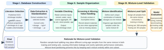
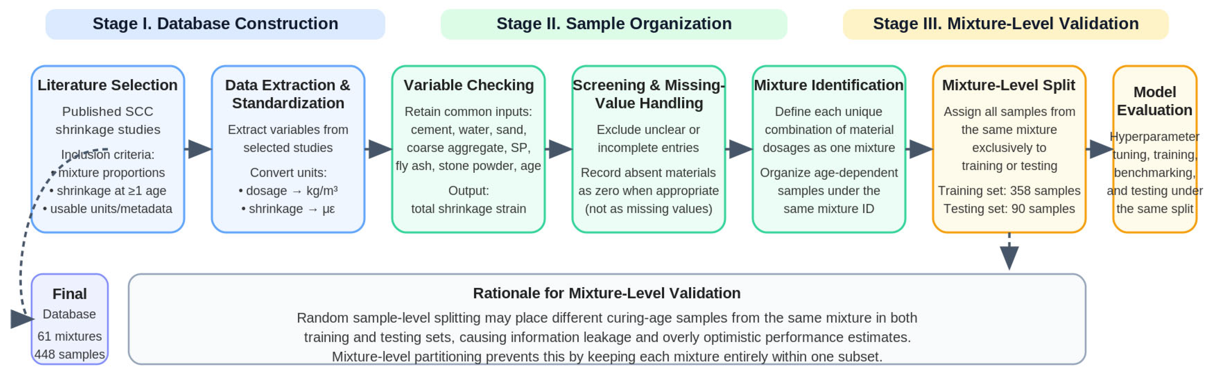
The SCC shrinkage database used in this study was constructed from published experimental studies rather than from a newly conducted casting program. Therefore, the methodological workflow focused on literature-based data collection, data screening, unit conversion, variable unification, sample organization, and mixture-level partitioning. This procedure was adopted to ensure that the compiled database could be used consistently for machine-learning model development and independent performance evaluation. The overall workflow of database construction and mixture-level validation is illustrated in Figure 1.

Figure 1. Workflow of database construction and mixture-level validation.

Experimental shrinkage data of self-compacting concrete were collected from six published sources [37,38,39,40,41,42]. The initial screening required that each selected study reported both mixture proportions and shrinkage measurements at one or more curing ages. A mixture design was defined as a unique combination of material dosages, including cement, water, sand, coarse aggregate, mineral admixtures, stone powder when applicable, and superplasticizer. For each mixture design, shrinkage values measured at different curing ages were treated as age-dependent data samples belonging to the same mixture. After screening and preprocessing, the final database contained 61 distinct mixture designs and 448 data samples.

The collected database includes both natural-sand SCC and manufactured-sand SCC. Mixtures containing stone powder were classified as manufactured-sand SCC, whereas mixtures without stone powder were classified as natural-sand SCC. The variables retained in the final database were selected according to two criteria: first, they had to be directly related to mixture design or curing age; second, they had to be consistently available across the selected data sources. Based on these criteria, cement content, water content, sand content, coarse aggregate content, superplasticizer dosage, fly ash content, stone powder content, and curing age were used as input variables, while total shrinkage strain was used as the output variable.

To improve consistency among different data sources, all material dosages were converted to kg/m³, and shrinkage strain was converted to με. Data samples with missing key mixture variables, unclear shrinkage values, or inconsistent units that could not be reliably converted were excluded. When a material component was not used in a specific mixture, such as stone powder in natural-sand SCC, its dosage was recorded as zero rather than treated as a missing value. This treatment preserved the distinction between the actual absence of a material component and incomplete data reporting. The availability of these variables in each data source is summarized in Table 1.

Table 1. Input variables in the SCC shrinkage dataset.

	Number of Mixtures	Cement	Water	Sand	Coarse Aggregate	Superplasticizer	Fly Ash	Stone Powder
Wang [37]	13	√	√	√	√	√		√
Cai [38]	9	√	√	√	√	√		√
Zhu [39]	12	√	√	√	√	√		√
Liu [40]	6	√	√	√	√	√	√
Luo [41]	12	√	√	√	√	√	√
Bai [42]	9	√	√	√	√	√	√

Note: Mixtures containing stone powder correspond to manufactured-sand SCC (MS-SCC), while mixtures without stone powder correspond to natural-sand SCC.

Because the database was compiled from published studies, not all experimental conditions were reported uniformly across the selected sources. In particular, environmental variables such as relative humidity, temperature, specimen size, and detailed curing condition were not consistently available. These variables were therefore not included as model inputs in the present study. This choice improves data consistency and practical usability because the retained input variables are commonly available from mixture proportioning data. However, it also limits the model’s applicability to the mixture and curing-age ranges represented in the compiled database. The influence of unavailable environmental variables is further discussed in Section 5.

Shrinkage datasets have an age-dependent structure that must be considered during data partitioning. Multiple shrinkage measurements are commonly obtained from the same mixture design at different curing ages. These samples are not fully independent because they share the same mixture composition and differ primarily in curing age. If random sample-level splitting is used, samples from the same mixture may appear in both the training and testing sets. In that case, the model may be evaluated on mixture proportions that have already been partially represented during training, leading to information leakage and overly optimistic estimates of generalization performance.

To avoid this problem, a mixture-level partitioning strategy was adopted in this study. All age-dependent data samples belonging to the same mixture design were assigned exclusively to either the training set or the testing set. Under this strategy, 358 data samples were used for model training, and the remaining 90 data samples were used for independent testing, corresponding to approximately 80% and 20% of the mixture designs, respectively. Unless otherwise stated, all model training, hyperparameter tuning, benchmarking, and performance evaluation in this study were conducted under this mixture-level data partitioning scheme. This strategy ensures that the testing set represents previously unseen mixture designs and provides a stricter assessment of model generalization capability for practical SCC shrinkage prediction.

2.2. Input/Output Variables and Data Preprocessing

The shrinkage prediction task in this study was formulated as a supervised regression problem. The objective was to establish a mapping between SCC mixture characteristics, curing age, and the corresponding total shrinkage strain. Based on the availability and consistency of the compiled database, eight input variables were selected: cement content, water content, sand content, coarse aggregate content, superplasticizer dosage, fly ash content, stone powder content, and curing age. The output variable was the total shrinkage strain measured at the corresponding curing age.

The selected input variables represent the main mixture-level factors that affect the shrinkage development of SCC. Cement, fly ash, and stone powder characterize the binder and powder system, which influences hydration products, pore structure, paste volume, and internal moisture transport. Water content is related to the water-to-binder ratio and the amount of evaporable water available during drying. Sand and coarse aggregate contents describe the aggregate skeleton, which restrains paste shrinkage and affects the overall volumetric stability of concrete. Superplasticizer dosage reflects the workability adjustment required for SCC, while curing age describes the time-dependent development of shrinkage. Therefore, the selected variables provide a practical and physically meaningful description of the main factors controlling SCC shrinkage.

These variables were also selected from the perspective of data availability and engineering usability. They are directly available from mixture proportioning data and are commonly reported in experimental studies and practical mixture design. Compared with derived variables or mechanical properties that are not consistently available across different sources, the use of mixture proportions and curing age allows the database to be unified without introducing excessive missing values. This is particularly important for a literature-compiled dataset with a limited number of mixture designs.

Some factors known to influence shrinkage, such as relative humidity, temperature, specimen size, curing condition, and detailed exposure environment, were not used as input variables because they were not consistently reported in the selected literature sources. Including these variables would have substantially reduced the usable dataset size and introduced additional uncertainty from missing-data treatment. Therefore, the present study focused on mixture proportions and curing age, which are more consistently available and easier to obtain in engineering practice. This choice improves the practical applicability of the proposed model, but it also means that the model should be used only within conditions reasonably represented by the compiled database. The influence of unavailable environmental variables is further discussed in Section 5.

$$x_{norm}={\displaystyle \frac{x-\overline{\mu }}{\sqrt{{\sigma }^2}}}$$

(1)

Before model training, all input variables were standardized using Z-score normalization to reduce the influence of differences in units and numerical scales among mixture components. To avoid information leakage, the mixture-level training/testing split was performed before normalization. The mean and standard deviation of each input variable were calculated using only the training set. These training-set statistics were then used to normalize both the training samples and the independent testing samples. No information from the testing set was used in the calculation of preprocessing parameters. In Equation (1), x_norm is the normalized value of a given input variable, x is the original value, and the mean and standard deviation are calculated from the training set. The output variable, total shrinkage strain, was retained in its original unit of microstrain (με) for model training and performance evaluation, so that MAE and RMSE remain directly interpretable from an engineering perspective.

2.3. Modeling Framework, Validation Protocol, and Performance Evaluation

The overall modeling framework was designed to ensure a clear separation among data partitioning, preprocessing, hyperparameter tuning, model training, ensemble construction, and independent testing. As illustrated in Figure 1, the mixture-level training/testing split was first performed at the mixture-design level. Data preprocessing parameters were then determined using only the training set, as described in Section 2.2. All model selection and hyperparameter tuning procedures were conducted within the training set, while the independent testing set was reserved exclusively for final model evaluation.

Four regression algorithms were selected as base learners: multilayer perceptron (MLP), support vector regression (SVR), decision tree (DT), and gradient boosting decision tree (GBDT). These models were chosen because they represent different learning mechanisms and can therefore provide complementary predictive behavior. MLP was used to capture smooth nonlinear relationships between mixture variables and shrinkage strain. SVR was included because it is suitable for nonlinear regression with limited sample sizes and can provide stable generalization through margin-based learning. DT was adopted to represent localized nonlinear rules and threshold-type interactions among mixture parameters. GBDT was included as a strong tree-based ensemble learner that can reduce prediction bias through sequential boosting. The diversity among these learners provides the basis for constructing heterogeneous ensemble models.

For each base learner, hyperparameters were selected using validation procedures conducted only within the training set. The independent testing set was not used during hyperparameter tuning, model selection, or ensemble configuration. For MLP, candidate hidden-layer structures, activation functions, and regularization coefficients were evaluated. For SVR, the kernel function, penalty parameter C, and insensitive loss parameter ε were tuned. For DT and GBDT, tree-related parameters such as tree depth, number of estimators, and splitting-related settings were examined. The final hyperparameter settings were selected according to validation performance and model stability within the training set. This procedure prevented the independent testing data from influencing model configuration.

After the construction of individual learners, ensemble models were developed to improve prediction robustness. Two types of ensemble strategies were considered. First, homogeneous ensemble models, including Bagging and AdaBoost, were used to examine whether repeated training of the same learner type could improve predictive performance. Second, heterogeneous ensemble models were constructed by combining different base learners. In particular, stacking was used as the main heterogeneous ensemble strategy. In the stacking framework, the predictions generated by base learners were used as input features for a meta-learner, which then produced the final shrinkage prediction.

To avoid information leakage during stacking, the meta-learner was trained using out-of-fold predictions generated within the training set. Specifically, the training set was divided into internal folds. For each fold, the base learners were trained using the remaining folds and were then used to predict the held-out fold. The resulting out-of-fold predictions were combined to form the meta-level training data. After the meta-learner was trained, the base learners were refitted using the full training set and then applied to the independent testing set to generate meta-level testing inputs. In this way, the meta-learner was trained without using base-learner predictions obtained from samples that had been used to fit the same base learners, and the independent testing set remained unseen until final evaluation.

The predictive performance of all candidate models was evaluated using the independent testing set defined by the mixture-level partitioning strategy. In addition to the machine-learning models, conventional shrinkage prediction models were implemented as benchmark methods when the required input parameters were available. All benchmark and data-driven models were evaluated using the same testing samples to ensure a fair and consistent comparison. Model performance was quantified using four statistical indicators: mean absolute error (MAE), root mean square error (RMSE), mean absolute percentage error (MAPE), and the coefficient of determination (R²). MAE and RMSE describe the absolute magnitude of prediction errors in microstrain, MAPE provides a dimensionless measure of relative prediction error, and R² evaluates the agreement between measured and predicted shrinkage values. Because the dataset contains multiple age-dependent samples from the same mixture design, all final evaluation metrics were calculated only on the independent testing set composed of unseen mixture designs. This protocol provides a stricter assessment of generalization capability than random sample-level splitting and ensures that data splitting, preprocessing, hyperparameter tuning, model training, ensemble construction, benchmarking, and independent evaluation remain methodologically separated throughout the study.

3. Learner Construction

3.1. Neural Network-Based Shrinkage Prediction Learner

The multilayer perceptron (MLP) model was used as one of the base learners because neural networks are capable of approximating nonlinear relationships between mixture parameters and shrinkage response. In the present study, cement content, water content, sand content, coarse aggregate content, fly ash content, stone powder content, superplasticizer dosage, and curing age were used as the eight input variables. The target output was the total shrinkage strain at the corresponding curing age. Accordingly, the MLP model consisted of eight input neurons and one output neuron.

Because the compiled SCC shrinkage database is relatively limited in size and contains heterogeneous mixture compositions, the network architecture and regularization setting must be carefully controlled to reduce overfitting. Therefore, the MLP hyperparameters were selected using validation procedures conducted only within the training set. The independent testing set was not used during network architecture selection or hyperparameter tuning. Four candidate hidden-layer structures, namely (15, 15), (15, 15, 15), (25, 15), and (25, 15, 10), were evaluated. The effects of different activation functions, including Logistic, Tanh, ReLU, and ELU, were also examined. In addition, the regularization coefficient α was selected according to validation performance.

The validation results showed that the hidden-layer structure of (25, 15, 10) provided comparatively better prediction stability than the other candidate architectures. Among the activation functions considered, ReLU produced the lowest validation error. The regularization coefficient was selected by minimizing the validation mean absolute error, and the optimal value was determined as α = 10⁻⁶. Therefore, the final MLP learner adopted a three-hidden-layer architecture of (25, 15, 10), the ReLU activation function, and a regularization coefficient of α = 10⁻⁶.

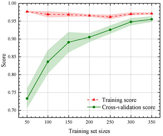
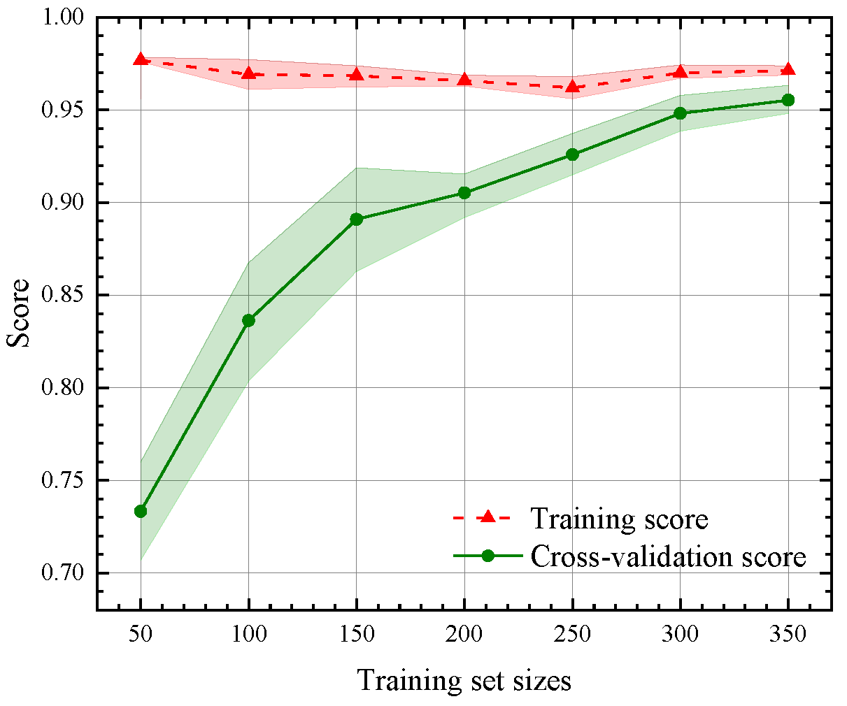
To further examine the influence of training sample size on the generalization behavior of the MLP model, a learning-curve analysis was performed using the training dataset. The learning curve and the independent testing prediction result of the MLP model are shown in Figure 2 and Figure 3, respectively. As shown in Figure 2, when the number of training samples increased from 50 to approximately 200, the training score decreased while the cross-validation score increased. This trend indicates that the gap between training and validation performance became smaller as more samples were included, suggesting reduced overfitting and improved generalization. When the number of training samples increased further from approximately 250 to 350, the cross-validation score tended to stabilize. This result suggests that, under the current mixture-level partitioning scheme, the available 358 training data samples provide a relatively stable basis for training the MLP learner.

Figure 2. Learning curve of the MLP model. The shaded area represents the variation range of the cross-validation score.

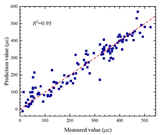
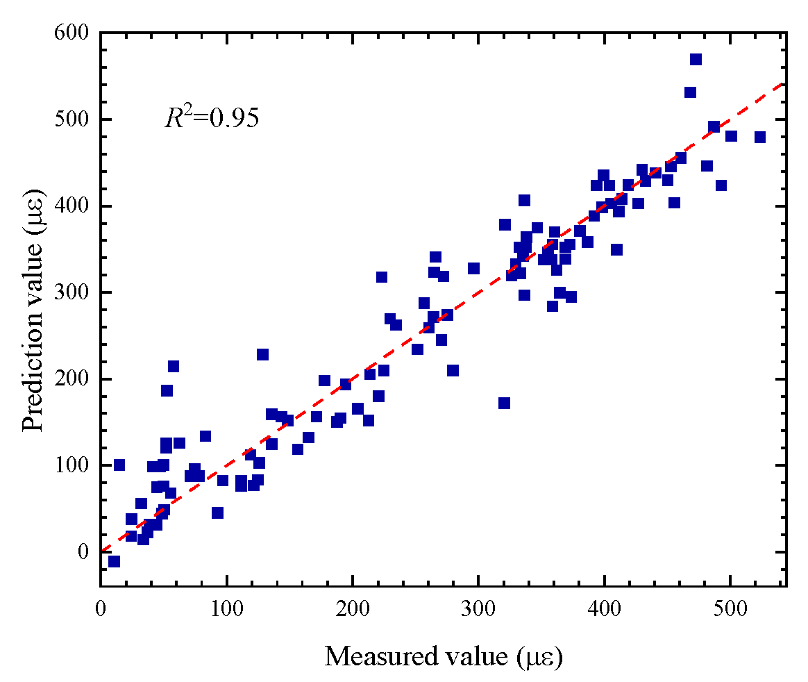
Figure 3. Predicted vs. measured shrinkage values of the MLP model. The red dashed line represents the y = x reference line.

After the architecture and hyperparameters were determined, the MLP model was trained using five-fold cross-validation within the training set and then evaluated on the independent testing set. As shown in Figure 3, the MLP model achieved a mean absolute error of 26.4 με and a mean absolute percentage error of 17.8% on the independent testing set.

The predicted shrinkage values were generally distributed around the y = x reference line, with R² = 0.95, indicating that the MLP model captured the overall nonlinear relationship between mixture variables, curing age, and shrinkage strain. Most relative errors were within approximately ±25%, and most absolute errors were within approximately ±50 με.

However, the standalone MLP learner still exhibited noticeable variability for some mixtures. This behavior is consistent with neural-network models trained on relatively small and heterogeneous datasets: although they can approximate complex nonlinear mappings, their prediction stability may depend strongly on data distribution and model configuration. Therefore, in this study, the MLP model was retained as a base learner rather than used as the final prediction model.

3.2. Support Vector Regression-Based Shrinkage Prediction Learner

Support vector regression (SVR) was selected as one of the base learners because it is suitable for nonlinear regression problems with relatively limited sample sizes. By introducing an insensitive loss function and maximizing the regression margin, SVR can balance fitting accuracy and generalization ability. This characteristic makes it useful for shrinkage prediction based on a compiled SCC database, where the number of mixture designs is limited and the relationships among mixture parameters, curing age, and shrinkage strain are nonlinear.

In this study, the standalone SVR learner used the same eight input variables as the MLP model: cement content, water content, sand content, coarse aggregate content, fly ash content, stone powder content, superplasticizer dosage, and curing age. The output variable was the total shrinkage strain at the corresponding curing age. It should be noted that the SVR model discussed in this subsection refers to the standalone SVR base learner. This is different from the final Stacking-SVR model discussed later, where SVR is used as the meta-learner to integrate the predictions of multiple base learners.

The performance of SVR is mainly affected by the kernel function, the penalty parameter C, and the insensitive loss parameter ε. The kernel function determines how nonlinear relationships are represented in the transformed feature space. The penalty parameter C controls the trade-off between the flatness of the regression function and the penalty imposed on prediction errors. The parameter ε defines the width of the insensitive zone, within which prediction errors are not penalized. Therefore, these hyperparameters were selected through validation procedures conducted only within the training set. The independent testing set was not used for kernel selection or hyperparameter tuning.

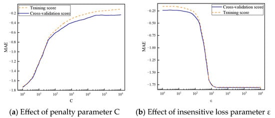
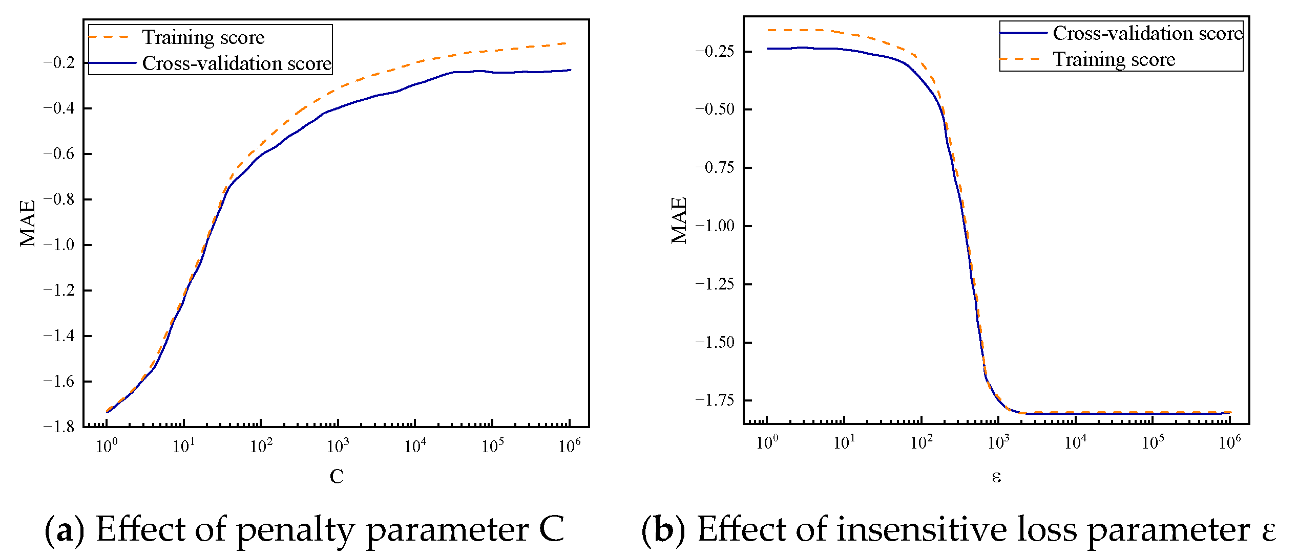
Four kernel functions were examined: linear, polynomial, radial basis function (RBF), and sigmoid kernels. Among these candidates, the RBF kernel gave the best validation performance. This result is reasonable because SCC shrinkage is controlled by nonlinear interactions among mixture composition, curing age, and material response, while the RBF kernel can describe smooth nonlinear variations without assuming a fixed empirical equation. After the RBF kernel was selected, the effects of C and ε were further examined using validation curves, as shown in Figure 4.

Figure 4. Validation curves for SVR hyperparameter selection.

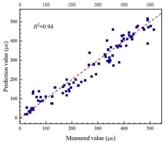
As shown in Figure 4a, increasing C improved the validation score at the initial stage, indicating that a larger penalty parameter allowed the SVR model to fit the training data more closely. However, when C exceeded 10⁴, the improvement became marginal and the validation curve gradually reached a plateau. Therefore, C = 10⁴ was selected for the final standalone SVR learner. The influence of ε is shown in Figure 4b. Larger ε values reduced the sensitivity of the model to training samples, but an excessively large insensitive zone caused a rapid decrease in prediction accuracy. Based on the validation results, the final value was set to ε = 0.2. After the kernel function and hyperparameters were determined, the optimized standalone SVR learner was trained using the training set and then evaluated on the independent testing set. The comparison between predicted and measured shrinkage values is shown in Figure 5.

Figure 5. Predicted versus measured shrinkage values of the standalone SVR learner. The red dashed line represents the y = x reference line.

As shown in Figure 5, the predicted shrinkage values are generally distributed around the y = x reference line, with R² = 0.94. This indicates that the standalone SVR learner captured the overall trend between mixture parameters, curing age, and shrinkage strain. However, the testing errors were still relatively large, with a mean absolute error of 35.3 με and a mean absolute percentage error of 26.6%. Several samples exhibited relatively large deviations, especially in the low-shrinkage range. This behavior can be partly explained by the definition of MAPE: when the measured shrinkage value is small, even a moderate absolute error can lead to a large percentage error. Therefore, the standalone SVR model was retained as a base learner rather than selected as the final prediction model.

3.3. Decision Tree-Based Shrinkage Prediction Learner

Decision tree regression (DT) was selected as one of the base learners because it can represent nonlinear and threshold-type relationships between input variables and shrinkage response. Unlike MLP and SVR, which construct relatively smooth nonlinear mappings, a decision tree recursively partitions the feature space into local regions and assigns a predicted shrinkage value to each terminal leaf node. This structure allows DT to capture localized interactions among mixture parameters, curing age, and shrinkage strain, which may be useful for heterogeneous SCC datasets compiled from multiple experimental sources.

In this study, the standalone DT learner used the same eight input variables as the MLP and SVR models: cement content, water content, sand content, coarse aggregate content, fly ash content, stone powder content, superplasticizer dosage, and curing age. The target output was the total shrinkage strain at the corresponding curing age. The DT model was implemented using the Decision Tree Regressor function in Scikit-Learn. During training, node splitting was performed by minimizing the impurity of the target values within each node, measured by the reduction in mean squared error.

Based on the training set containing 358 data samples, the constructed decision tree reached a maximum depth of 14 and consisted of 328 leaf nodes. This structure indicates that the standalone DT learner had high flexibility and was able to represent detailed local patterns in the training data. At the same time, such a deep tree may be sensitive to local fluctuations and may exhibit high variance when applied to unseen mixture designs. Therefore, the revised manuscript does not claim that overfitting of the standalone DT learner was fully controlled. Instead, the DT model is explicitly treated as a flexible but potentially high-variance base learner. Its purpose is to provide localized nonlinear prediction information for the subsequent ensemble models rather than to serve as the final shrinkage prediction model. This interpretation is further supported in the following ensemble-model comparison, where Bagging, Boosting, and Stacking strategies are evaluated to reduce the instability associated with individual learners.

After model construction, the standalone DT learner was evaluated on the independent testing set. The comparison between predicted and measured shrinkage values is shown in Figure 6.

Figure 6. Predicted versus measured shrinkage values of the standalone DT learner. The red dashed line represents the y = x reference line.

Nevertheless, several testing samples still showed relatively large deviations, especially in the lower shrinkage range. This behavior may be related to the sensitivity of decision trees to local data distribution. Because each terminal leaf prediction is determined by the training samples falling within a specific partitioned region, sparse samples or locally irregular shrinkage development can lead to unstable predictions for unseen mixtures. The larger relative deviations were mainly associated with low-magnitude shrinkage predictions, where even moderate absolute errors can produce relatively high percentage errors. Because curing condition and environmental variables were not uniformly available in the compiled database, these deviations cannot be attributed to a single mixture parameter with sufficient confidence. Overall, DT was used primarily as a base learner rather than as the final prediction model.

As shown in Figure 6, the DT model achieved a testing MAE of 19.27 με and a testing MAPE of 11.6%. Most prediction errors were within approximately ±50 με, and the corresponding relative errors were mainly within approximately ±20%. These results indicate that the standalone DT learner captured part of the nonlinear relationship between mixture composition, curing age, and shrinkage strain. Compared with the standalone MLP and SVR learners, DT produced lower testing errors on this dataset, suggesting that localized splitting rules were effective for describing some mixture-dependent shrinkage patterns.

4. Development of the SCC Shrinkage Prediction Model

4.1. Homogeneous Ensemble Models

The use of ensemble models was partly motivated by the limitations of individual learners discussed in Section 3. In particular, the standalone DT learner can capture localized nonlinear patterns, but its deep tree structure may also lead to high variance when applied to unseen mixture designs. Homogeneous ensemble learning provides a way to improve prediction robustness by combining multiple sub-learners trained using the same learning algorithm. In this study, Bagging and AdaBoost were first examined for MLP, DT, and SVR learners to evaluate whether repeated training of the same learner type could improve testing performance under the mixture-level validation scheme.

For the homogeneous ensemble models, the ensemble size was treated as an important hyperparameter. The ensemble size for the MLP-based ensemble was determined through repeated validation trials within the training set, whereas the ensemble sizes for the DT- and SVR-based ensembles were selected using grid-search procedures within the training set. The independent testing set was used only for final evaluation. The testing errors of the homogeneous ensemble models are summarized in Table 2.

Table 2. Testing errors of homogeneous ensemble models.

Learner	AdaBoost			Bagging
	Number	MAE	MAPE	Number	MAE	MAPE
MLP	10	28.1	16.8%	10	27.8	17.4%
DT	20	22.2	15.9%	20	18.9	15.6%
SVR	100	35.9	36.3%	200	33.6	38.2%

As shown in Table 2, the homogeneous ensemble strategies did not consistently improve the testing performance of all learner types. For the MLP-based models, AdaBoost and Bagging produced similar testing errors, with MAPE values of 16.8% and 17.4%, respectively. For the DT-based models, Bagging reduced the MAE from 22.2 με for AdaBoost-DT to 18.9 με for Bagging-DT, while the MAPE values remained close. For the SVR-based models, both AdaBoost-SVR and Bagging-SVR showed relatively large MAPE values, indicating that simply repeating the same SVR learner did not provide effective improvement for this dataset. Because no statistical significance test was conducted specifically for the pairwise comparison between AdaBoost and Bagging in Table 2, the differences are interpreted only in terms of their numerical testing errors. Overall, the results suggest that homogeneous ensembles based on a single learner type provide limited and inconsistent improvement.

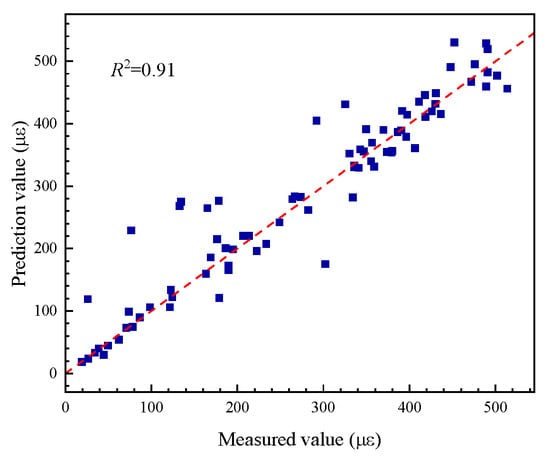
In addition to Bagging and AdaBoost, a gradient boosting decision tree (GBDT) model was constructed as a stronger tree-based ensemble learner. Unlike Bagging, which mainly reduces variance by averaging multiple learners trained on resampled data, GBDT builds trees sequentially so that each new tree focuses on reducing the residual errors of the previous ensemble. In this study, the maximum depth of each regression tree was set to 3, and the number of trees was set to 300. The predicted and measured shrinkage values of the GBDT model are compared in Figure 7.

Figure 7. Predicted versus measured shrinkage values of the GBDT model. The red dashed line represents the y = x reference line.

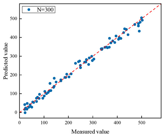
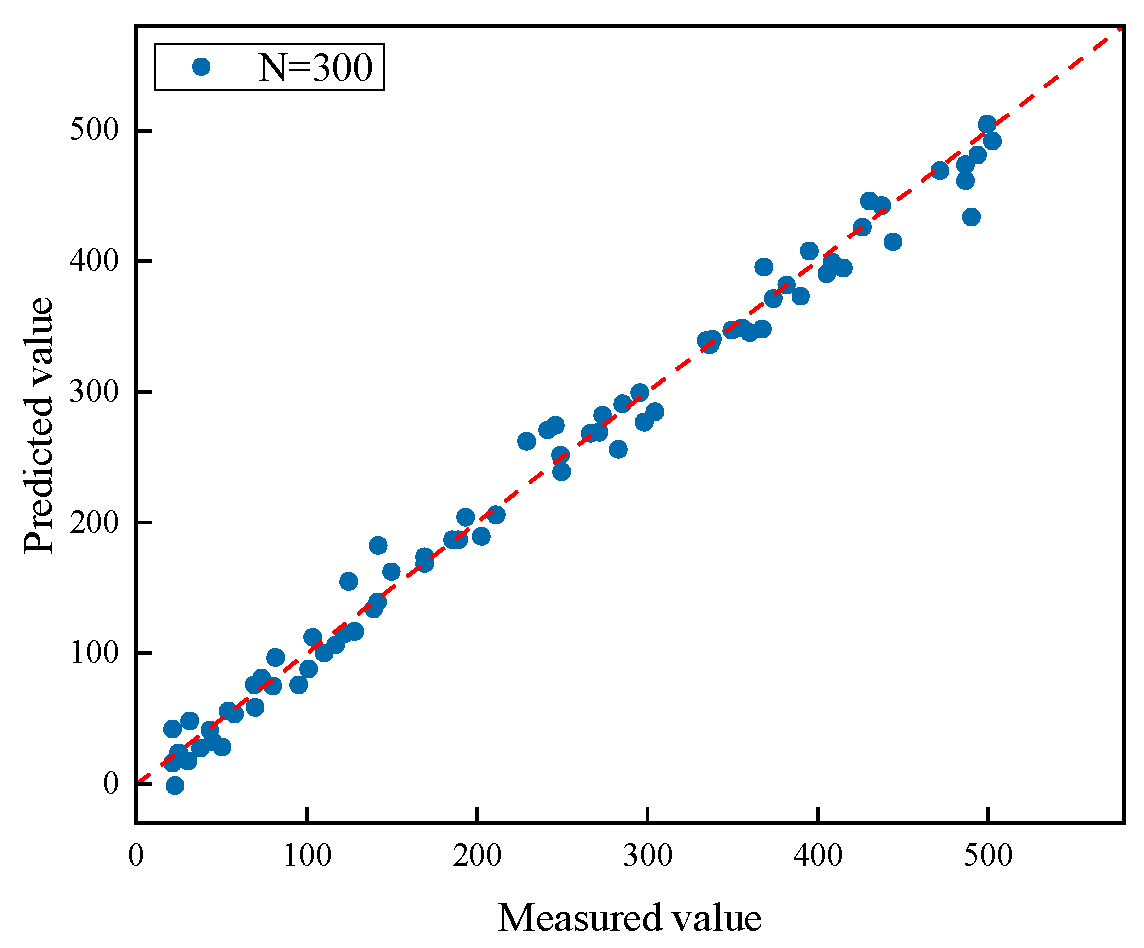
As shown in Figure 7, the GBDT model achieved a testing MAE of 10.76 με and a testing MAPE of 10.7%. Compared with the standalone DT learner discussed in Section 3.3, GBDT markedly reduced MAE and slightly reduced MAPE, indicating that boosting improved the generalization behavior of tree-based prediction under the mixture-level testing scheme. However, although GBDT provided better performance than the standalone tree model, its accuracy was further examined against heterogeneous ensemble and stacking models in the following section.

4.2. Heterogeneous Ensemble Shrinkage Prediction Models

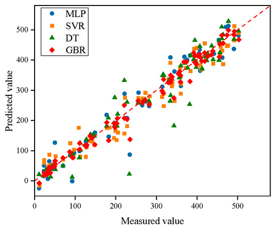
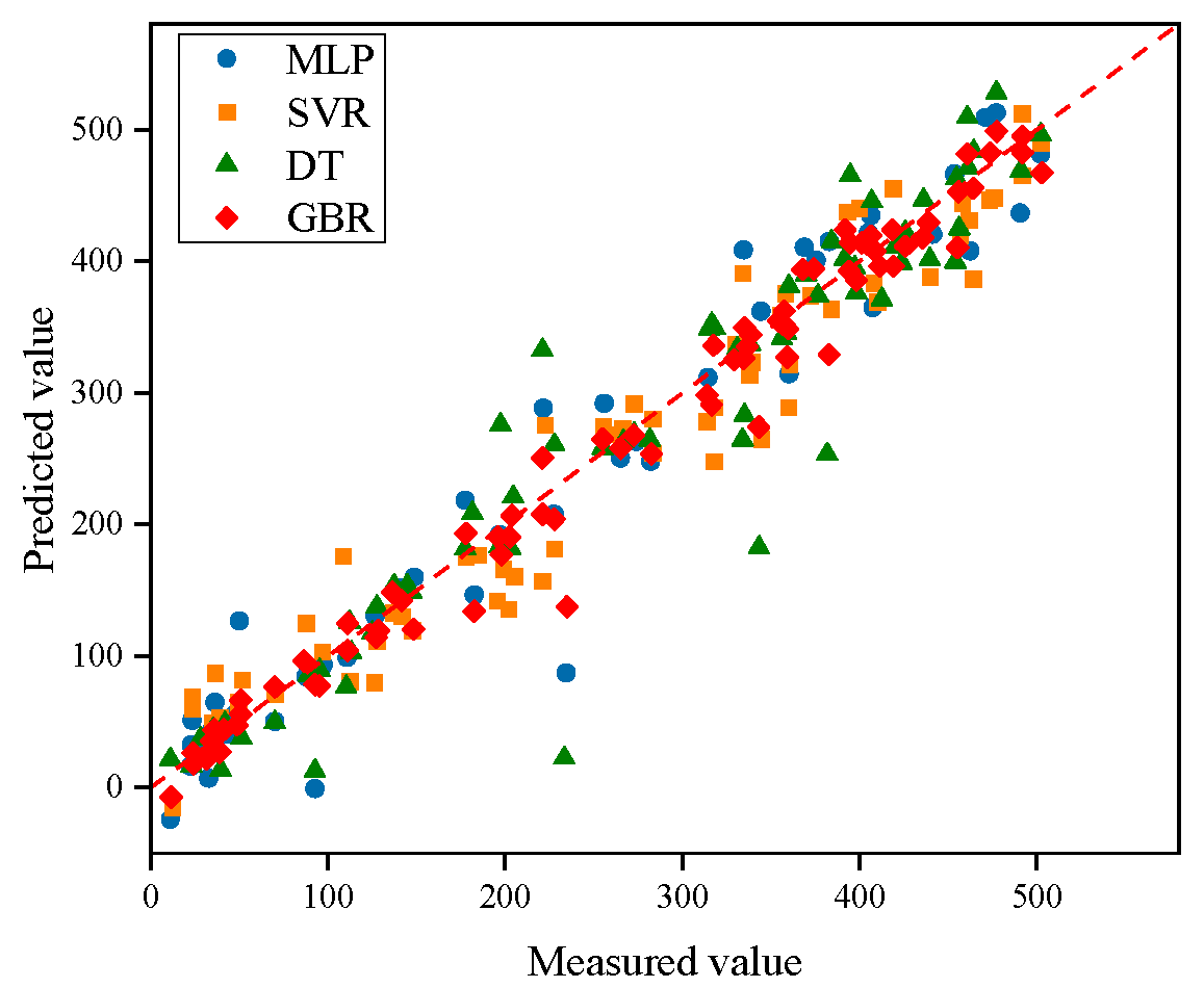
Although homogeneous ensemble models can improve prediction robustness by combining multiple learners of the same type, their improvement may be limited when the sub-learners have similar error patterns. To further increase model diversity, heterogeneous ensemble models were developed by combining different learning algorithms. In this study, the predictions generated by MLP, SVR, DT, and GBDT were integrated using averaging, weighted averaging, and stacking strategies. The purpose of this section is to compare different heterogeneous ensemble structures and identify promising candidate models for the final evaluation in Section 4.3.

First, a simple averaging ensemble was constructed by taking the arithmetic mean of the predictions produced by the four base learners. This method does not introduce additional trainable parameters and therefore provides a straightforward baseline for heterogeneous model combination. The averaging ensemble achieved a testing MAE of 16.3 με and a MAPE of 13.0%. Compared with some standalone learners, the averaging strategy reduced prediction error to a certain extent. However, because it assigns equal importance to all base learners, it cannot account for differences in the accuracy, stability, and error patterns of individual learners.

Second, a weighted ensemble was constructed by assigning different weights to the predictions of the base learners. In this formulation, the outputs of the base learners are used as input features, and the measured shrinkage values are used as regression targets to estimate the combination weights. This approach is expressed in Equation (2).

$$out=a_1\times MLP+a_2\times SVR+a_3\times DT+b$$

(2)

Equation (2) defines the weighted combination formulation. The outputs of the base learners serve as input features for the combination model, and the regression coefficients represent the estimated weights of the corresponding learners. From this perspective, the weighted ensemble can be regarded as a simplified stacking formulation, in which a linear meta-model is used to combine the predictions of different base learners. The prediction results of the weighted heterogeneous ensemble based on the four base learners are shown in Figure 8.

Figure 8. Predicted versus measured shrinkage values of the weighted heterogeneous ensemble based on four base learners. The red dashed line represents the y = x reference line.

As shown in Figure 8, the weighted heterogeneous ensemble achieved a testing MAE of 17.8 με and a MAPE of 14.0%. This result indicates that a simple linear weighting of base-learner outputs did not fully exploit the complementary information among different models. One possible reason is that the relationship between base-learner predictions and the measured shrinkage response may still be nonlinear. Therefore, a more flexible stacking strategy was further examined.

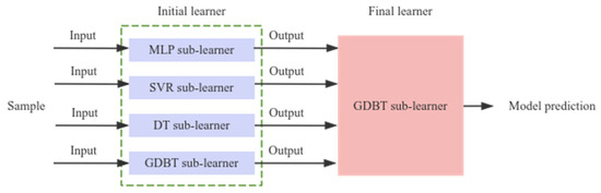
In the stacking framework, each input sample is first processed by the base learners, and their predictions are then used as meta-level input features for a final learner. This structure allows the final learner to identify systematic differences among base learners and combine their predictions more adaptively. The schematic diagram of the stacking framework is shown in Figure 9.

Figure 9. Schematic diagram of the stacking ensemble framework.

Several stacking configurations were examined by using different algorithms as the final learner. Compared with the simple averaging and linear weighted ensemble strategies, the stacking framework provided a more flexible way to combine base-learner predictions. Among the examined configurations, the SVR-based meta-learner showed promising performance in the preliminary comparison. This may be because the meta-level feature space formed by base-learner predictions is relatively low-dimensional, and SVR is suitable for learning stable nonlinear relationships under limited sample conditions.

However, the results in this section are used only to screen promising heterogeneous ensemble configurations. To reduce the influence of dataset-dependent variability and to select the final model more reliably, the candidate models were further compared under a consistent cross-validation and independent testing protocol in Section 4.3. Therefore, the Stacking-SVR configuration was retained as a promising candidate for the final model comparison, while the final selection of the SCC shrinkage prediction model was based on the comparative results reported in the following section.

4.3. Determination of the Final Ensemble Shrinkage Prediction Model

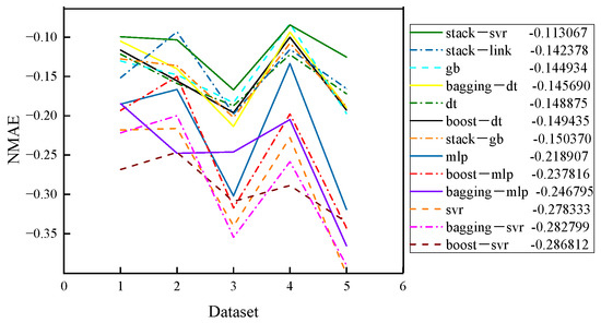
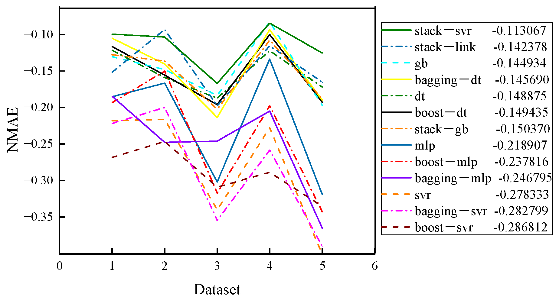
To determine the final SCC shrinkage prediction model, the candidate models developed in the previous sections were compared using a consistent validation and testing procedure. Candidate models were first screened using repeated cross-validation within the training set. This step was used to reduce the influence of data partition variability during model comparison and to identify models with relatively stable prediction performance. The independent testing set was not used during this candidate-screening stage. The cross-validation comparison of candidate models is shown in Figure 10.

Figure 10. Cross-validation error comparison of candidate shrinkage prediction models.

As shown in Figure 10, the candidate models exhibited different levels of prediction error under the repeated validation procedure. Models with lower validation errors were retained for final independent testing. This screening step was not used as the sole basis for final model selection; instead, the top candidate models were subsequently retrained using the training set and evaluated on the independent testing set defined by the mixture-level partitioning strategy. The independent testing results of the retained candidate models are summarized in Table 3.

Table 3. Testing errors of candidate models under mixture-level validation.

	Stack-SVR	Stack-Linear	GBDT	Bagging-DT	DT	AdaBoost-DT	Stack-GBDT
MAE	13.6	18.0	14.2	15.7	19.6	16.9	16.3
MAPE	7.5	10.1	8.4	8.9	11.6	10.2	8.5

As shown in Table 3, the Stack-SVR model achieved the lowest MAPE among the retained candidate models, with a testing MAE of 13.6 με and a testing MAPE of 7.5%. Compared with the standalone DT model, the Stack-SVR model reduced MAPE from 11.6% to 7.5%, corresponding to a relative reduction of approximately 35.3%. Compared with GBDT and Stack-GBDT, the MAPE was reduced from 8.4% and 8.5% to 7.5%, corresponding to relative reductions of approximately 10.7% and 11.8%, respectively. These results indicate that the stacking framework with SVR as the meta-learner provided the best overall testing performance under the mixture-level validation strategy.

Although Stack-SVR showed the best accuracy among the evaluated models, the improvement should be interpreted together with model complexity. Simpler models such as GBDT and Bagging-DT also achieved competitive testing errors and may be useful for rapid preliminary screening. However, for the purpose of achieving the highest prediction accuracy within the present mixture-level validation framework, Stack-SVR was selected as the final SCC shrinkage prediction model. Subsequent analyses therefore focus on the stability, applicability, and engineering interpretation of the Stack-SVR model.

5. Discussion

5.1. Evaluation of the Final Stacking-SVR Shrinkage Prediction Model

5.1.1. Stability Analysis

After the Stack-SVR model was selected as the final prediction model in Section 4.3, its engineering reliability was further examined from three aspects: stability, accuracy, and applicability range. For practical SCC production, mixture proportions may deviate from target values because of batching errors, material moisture variation, and construction-site adjustment. Therefore, a shrinkage prediction model should not be overly sensitive to small changes in input variables. To evaluate the stability of the final Stack-SVR model, perturbations were introduced into the input variables of the testing samples, and the corresponding changes in model output were examined. The perturbation radii used in the analysis are listed in Table 4.

Table 4. Perturbation radii of input variables used for stability analysis (unit: kg/m³).

	Cement	Water	Fly Ash	Sand	Coarse Aggregate	Stone Powder	Superplasticizer
Sample mean	424	176	39	719	1059	34	3.0
Perturbation radius	13	5	1	21	31	20	0.1

The stability of the model was quantified using the error amplification factor defined in Equation (3), which describes the ratio between the relative change in model output and the relative perturbation in model input. The perturbation procedure was repeated ten times for the independent testing set, and the mean and variance of the error amplification factor were calculated for each repeated test. The results are summarized in Table 5.

$$C_p=\left|{\displaystyle \frac{\Delta y}{y}}/{\displaystyle \frac{\Delta x}{x}}\right|=\left|{\displaystyle \frac{f(x)-f(x^{*})}{f(x)}}\right|/\left|{\displaystyle \frac{\Delta x}{x}}\right|$$

(3)

Equation (3) defines the error amplification factor (also referred to as a condition number in this context), where C_p is the amplification factor, f(x) is the prediction without perturbation, f(x*) is the prediction after perturbation, Δx is the applied perturbation, and x is the original input vector.

Table 5. Error amplification factor Cp under repeated input perturbations.

	Test Set-1	Test Set-2	Test Set-3	Test Set-4	Test Set-5	Test Set-6	Test Set-7	Test Set-8	Test Set-9	Test Set-10
Average	1.77	1.73	1.16	1.29	2.79	1.97	2.60	1.09	4.61	4.8
Variance	2.36	2.42	1.88	1.83	3.86	2.84	3.58	1.68	3.89	2.83

Table 5. Error amplification factor Cp under repeated input perturbations.

	Test Set-1	Test Set-2	Test Set-3	Test Set-4	Test Set-5	Test Set-6	Test Set-7	Test Set-8	Test Set-9	Test Set-10
Average	1.77	1.73	1.16	1.29	2.79	1.97	2.60	1.09	4.61	4.8
Variance	2.36	2.42	1.88	1.83	3.86	2.84	3.58	1.68	3.89	2.83

5.1.2. Accuracy Comparison with Conventional Shrinkage Models

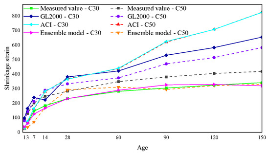
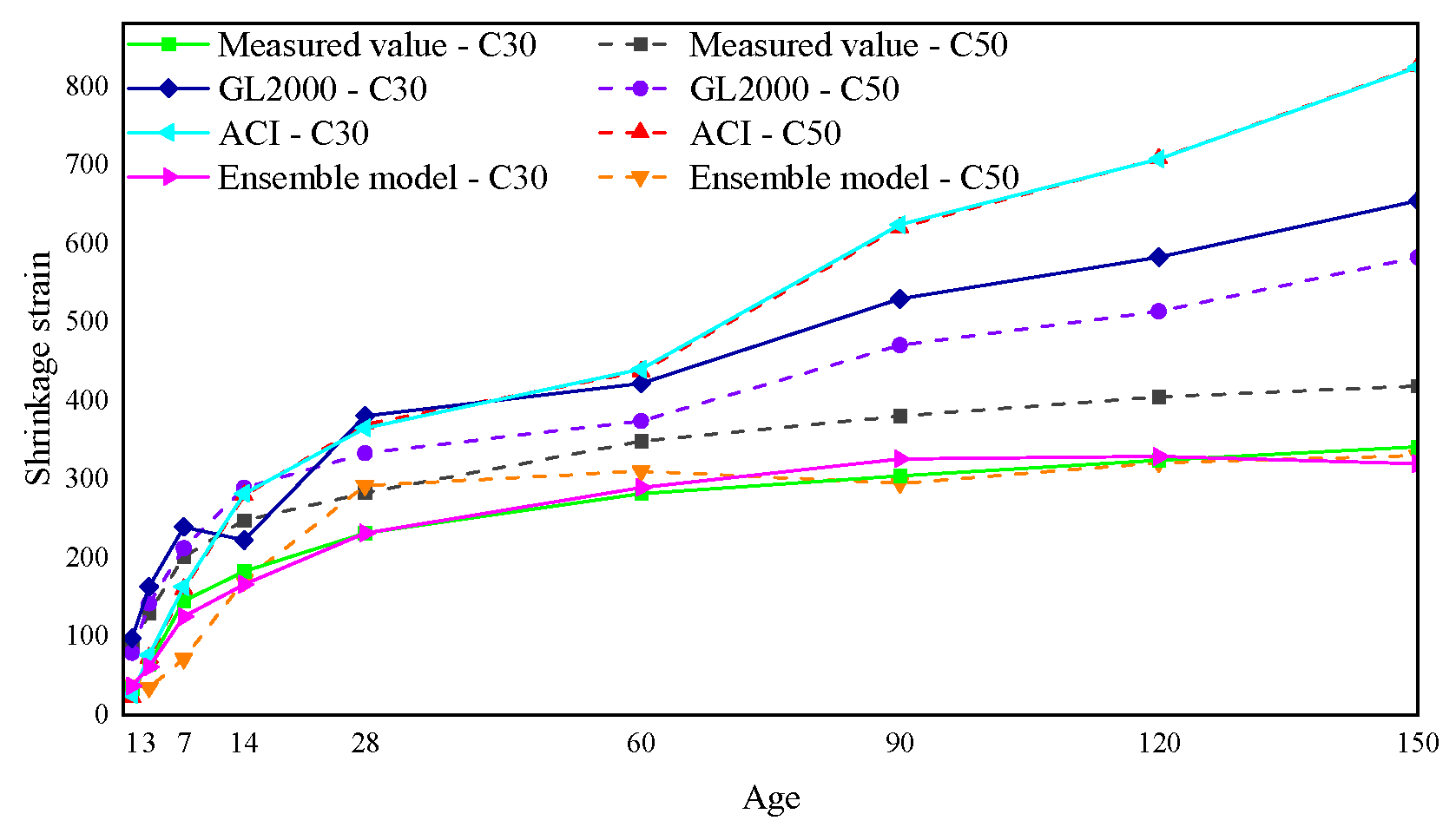
As shown in Table 5, the average amplification factors ranged from 1.09 to 4.80, and the corresponding variances were below 4.0 in all repeated tests. These results indicate that the Stack-SVR model did not exhibit excessive output amplification under the selected input perturbation levels. To further examine the predictive accuracy of the final model, the Stack-SVR model was applied to shrinkage data reported in Ref. [43]. The GL2000 and ACI shrinkage models were also used for comparison when the required input parameters were available. The comparison between measured shrinkage values and the predictions obtained from Stack-SVR, GL2000, and ACI is shown in Figure 11.

Figure 11. Comparison between measured shrinkage values and predictions obtained from Stack-SVR, GL2000, and ACI models.

As shown in Figure 11, for the C30 mixture containing 10% stone powder, the Stack-SVR prediction follows the measured shrinkage development trend over the examined age range. The GL2000 and ACI models provide predictions close to the measured values at early ages, but their deviations become more evident after approximately 28 days. This difference suggests that conventional empirical models may have difficulty capturing the later-age shrinkage development of SCC mixtures containing stone powder.

For the C50 mixture, the Stack-SVR model slightly underestimates shrinkage within the first 28 days, while the GL2000 and ACI models are closer to the measured values in the early-age range. Between 28 and 60 days, the three models provide relatively similar predictions. After 60 days, the Stack-SVR prediction remains closer to the measured development trend, whereas the GL2000 and ACI models continue to show an increasing tendency that gradually deviates from the measured shrinkage curve.

These comparison results indicate that the Stack-SVR model can reasonably capture the shrinkage development characteristics of SCC and manufactured-sand SCC in the examined cases. Nevertheless, this comparison should be interpreted as an application-oriented accuracy check rather than a comprehensive external validation, because it is based on selected mixtures from Ref. [43]. A broader external validation using more independent SCC shrinkage datasets would further strengthen the generality of the proposed model.

5.1.3. Applicability Range Analysis

For engineering application, it is necessary to define the applicable range of the prediction model. Because the Stack-SVR model was trained using a compiled database, its reliable use should be limited to the parameter ranges represented by that database. Based on the collected data, the main variable ranges include a water-to-binder ratio of 0.32–0.53, a stone powder content of 0–50 kg/m³, an aggregate content of 900–1200 kg/m³, a sand content of 600–800 kg/m³, and a fly ash content of 0–75 kg/m³. Predictions outside these ranges should be treated with caution because they involve extrapolation beyond the training data distribution.

To further examine the influence of water-to-binder ratio on model behavior, shrinkage predictions were generated for mixtures containing 15% stone powder with water-to-binder ratios ranging from 0.25 to 0.60. The results are shown in Figure 12. When the water-to-binder ratio is 0.25 or 0.30, the predicted shrinkage development deviates from the expected physical trend. When the water-to-binder ratio increases to 0.55 or 0.60, the predicted curves become very close to each other, suggesting reduced model sensitivity in this extrapolated region. Based on this analysis, the practical applicable range of the water-to-binder ratio is recommended as approximately 0.35–0.55.

Figure 12. Predicted shrinkage development of mixtures with 15% stone powder under different water–to–binder ratios.

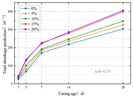
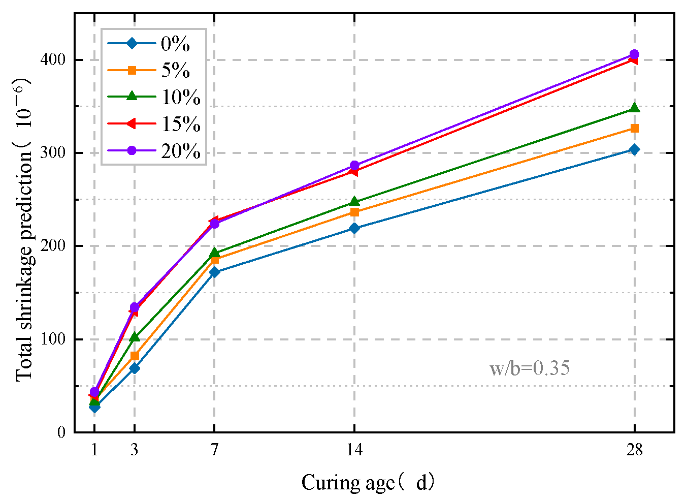
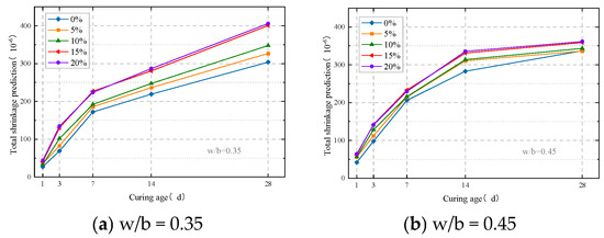
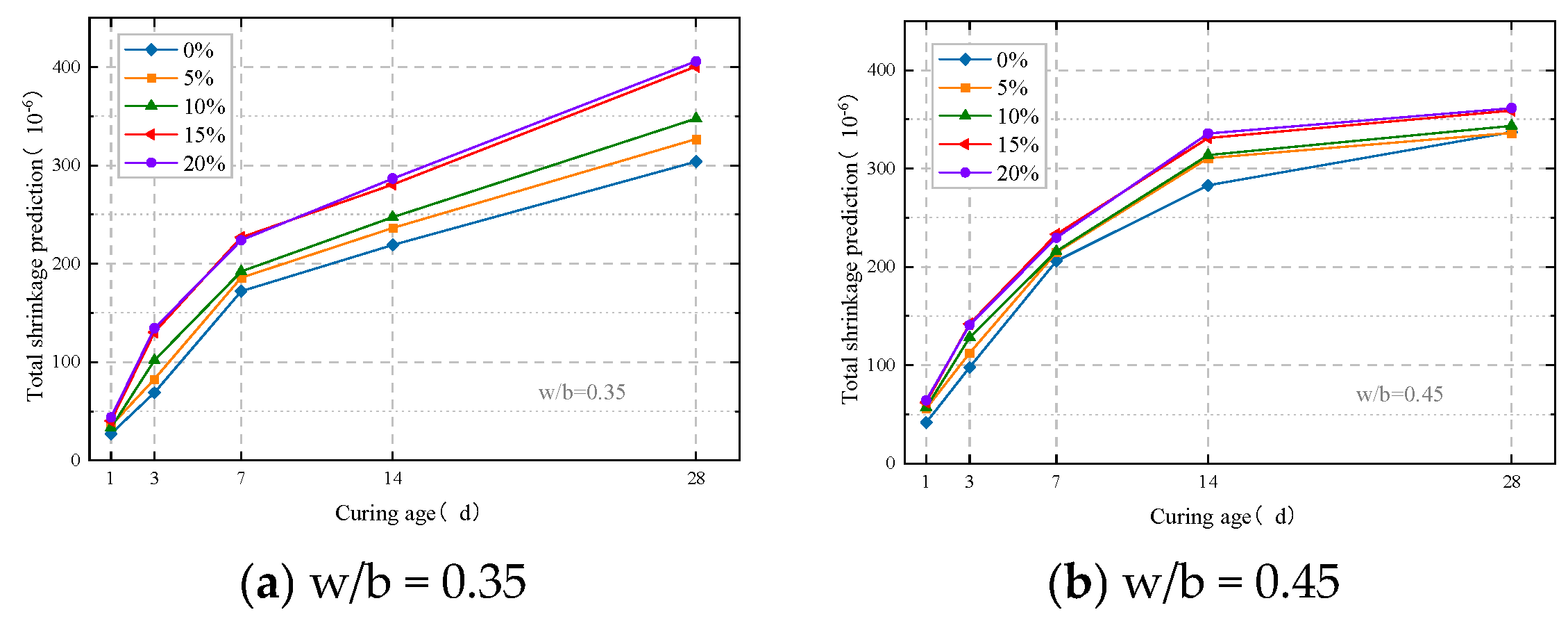
The influence of stone powder content was also examined under representative water-to-binder ratios, as shown in Figure 13. The predicted shrinkage curves vary with stone powder content, indicating that the model captures the influence of powder-system changes on shrinkage development. However, the interpretation of stone powder effects should remain limited to the dosage range covered by the compiled database. Overall, the stability, accuracy, and applicability analyses show that the final Stack-SVR model has practical potential for SCC shrinkage prediction under mixture-level validation. At the same time, the model should not be regarded as a universal replacement for experimental testing or code-based design checks. Its predictions are most reliable within the database-supported range, and future work should incorporate larger external datasets and environmental variables such as relative humidity, temperature, specimen size, and curing condition to improve generalization.

Figure 13. Predicted shrinkage development for applicability analysis under different stone powder contents at w/b = 0.35 and 0.45.

5.2. Validation and Engineering Application of the SCC Shrinkage Model

To further examine the engineering applicability of the final Stack-SVR shrinkage prediction model, the model was applied to a set of representative manufactured-sand SCC mixtures. The mixture proportions used for this application analysis are listed in Table 6. These mixtures were selected based on Ref. [43] and include three water-to-binder ratios (w/b = 0.45, 0.50, and 0.60) and three stone powder contents (0%, 10%, and 15%). For each mixture, shrinkage development within 150 days was predicted. The purpose of this analysis was to evaluate whether the final Stack-SVR model could produce reasonable shrinkage development trends under controlled variations in key mixture parameters.

Table 6. Mixture proportions used for engineering application analysis (unit: kg/m³).

Mixture ID	Cement	Water	Sand	Coarse Aggregate	Superplasticizer	Stone Powder	Fly Ash
M1-0.60-0%	280	165	768	1064	4.08	0.0	60
M1-0.60-10%	280	165	768	1064	4.08	76.8	60
M1-0.60-15%	280	165	768	1064	4.08	115.2	60
M2-0.50-0%	330	163	738	1064	8.00	0.0	70
M2-0.50-10%	330	163	738	1064	8.00	73.8	70
M2-0.50-15%	330	163	738	1064	8.00	110.7	70
M3-0.45-0%	370	165	682	1064	10.81	0.0	100
M3-0.45-10%	370	165	682	1064	10.81	68.2	100
M3-0.45-15%	370	165	682	1064	10.81	102.3	100

5.2.1. Shrinkage Prediction Under Different Water-to-Binder Ratios

The selected mixtures allow the effects of water-to-binder ratio and stone powder content to be examined separately. Figure 14 shows the predicted shrinkage development under different water-to-binder ratios for stone powder contents of 0%, 10%, and 15%. In all cases, predicted shrinkage increases with curing age and gradually approaches a plateau. This trend is consistent with the typical time-dependent development of concrete shrinkage, in which shrinkage grows rapidly at early ages and then slows as moisture loss and hydration-related deformation gradually stabilize.

Figure 14. Engineering application analysis of predicted shrinkage development under different water-to-binder ratios at stone powder contents of 0%, 10%, and 15%.

The influence of water-to-binder ratio is most evident during the early and intermediate age ranges. Within the first 60 days, the mixtures with w/b = 0.45 show a higher shrinkage growth rate than those with w/b = 0.50 and w/b = 0.60. After approximately 60 days, the shrinkage curve for w/b = 0.45 enters a slower growth stage. For w/b = 0.50 and w/b = 0.60, shrinkage increases more gradually within the first 90 days and then also transitions into a slow-growth stage. After 90 days, the predicted shrinkage values under the three water-to-binder ratios become relatively close. This predicted behavior indicates that the final Stack-SVR model captures the coupled influence of water content, binder content, and curing age on shrinkage development.

5.2.2. Shrinkage Prediction Under Different Stone Powder Contents

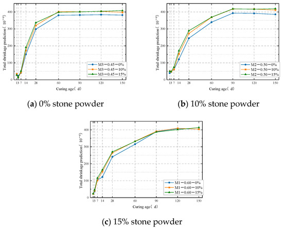
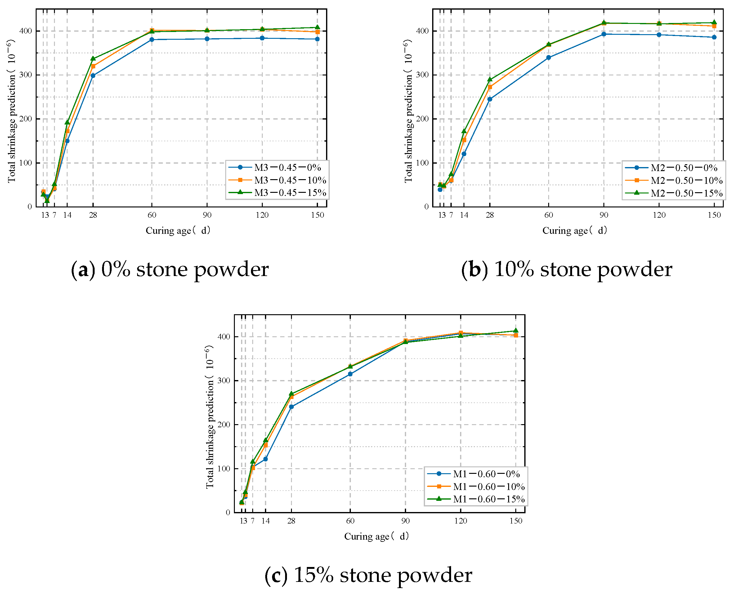
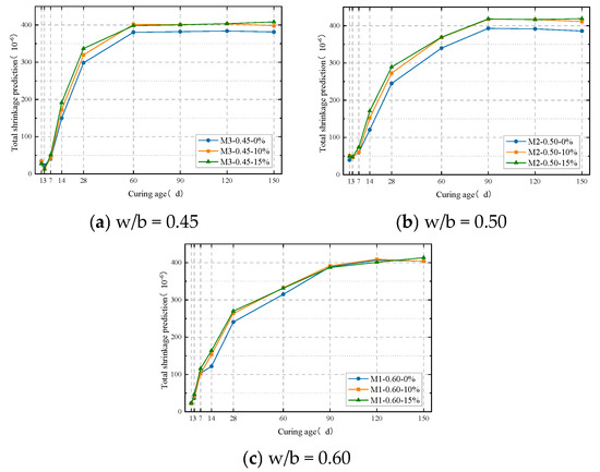
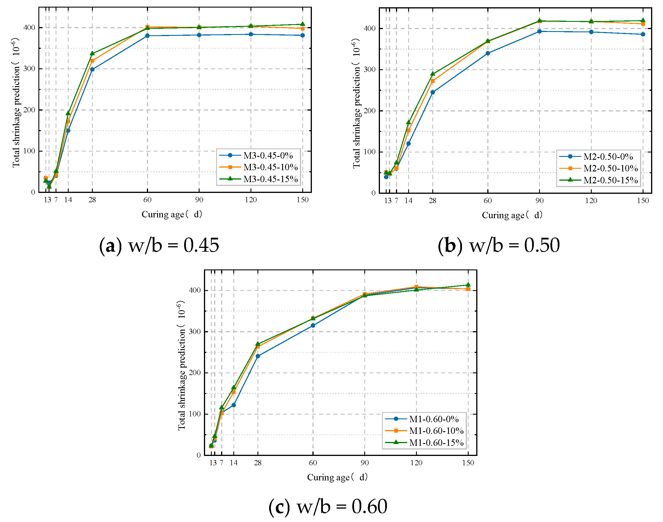
Figure 15 presents the predicted shrinkage development under different stone powder contents for water-to-binder ratios of 0.45, 0.50, and 0.60. As shown in Figure 15, the influence of stone powder content follows a generally consistent age-dependent pattern. In all cases, the predicted shrinkage increases rapidly within the first 28 days, then the growth rate decreases, and the curves gradually approach a plateau after approximately 60–90 days. This indicates that the model captures the dominant time-dependent shrinkage trend while also reflecting changes caused by stone powder content.

Figure 15. Engineering application analysis of predicted shrinkage development under different stone powder contents at w/b = 0.45, 0.50, and 0.60.

For the mixtures with w/b = 0.60, the predicted shrinkage curves under different stone powder contents are relatively close. This indicates that the sensitivity of predicted shrinkage to stone powder content becomes weaker at a higher water-to-binder ratio. Overall, the application analysis shows that the Stack-SVR model can generate physically reasonable shrinkage development trends under controlled variations in water-to-binder ratio and stone powder content. However, the results should be interpreted within the scope of the compiled database. The proposed Stack-SVR model should therefore be regarded as an engineering-support tool for shrinkage estimation rather than a substitute for laboratory testing or code-based durability design.

For the mixtures with w/b = 0.45, the predicted shrinkage generally increases with increasing stone powder content. At 28 days, the predicted shrinkage of the mixture containing 10% stone powder is approximately 23 με higher than that of the mixture without stone powder, while the difference between 10% and 15% stone powder is relatively small. For the mixtures with w/b = 0.50, the predicted shrinkage values of the 10% and 15% stone powder mixtures are clearly higher than those of the 0% stone powder mixture. At 28 days, the predicted shrinkage of the 10% stone powder mixture is approximately 30 με higher than that of the 0% stone powder mixture, whereas the difference between 10% and 15% stone powder remains limited.

5.3. Comparison with Previous Studies and Engineering Implications

To further clarify the contribution and application scope of the present study, a comparison with recent machine-learning-based studies on concrete shrinkage prediction and concrete-property prediction is summarized in Table 7. The comparison focuses on the prediction target, modeling strategy, validation feature, main advantages, limitations, and relevance to engineering application.

Table 7. Comparison between the present study and recent machine-learning-based concrete shrinkage/property prediction studies.

Study	Prediction Target and Material	Main Modeling Approach	Validation/Data Organization Feature	Main Advantage and Limitation	Difference and Contribution of the Present Study
Behnood and Golafshani [17]; Young and Hall [18]	Drying shrinkage/concrete shrinkage behavior	Data-driven and machine-learning models	Prediction models developed from collected concrete shrinkage datasets	Advantage: demonstrated the feasibility of ML for nonlinear shrinkage prediction. Limitation: mainly focused on general concrete shrinkage; mixture-level leakage control was not the central issue.	The present study focuses specifically on SCC shrinkage and adopts mixture-level validation to evaluate prediction for unseen mixture designs.
Wang and Xu [19]; Liu and Li [21]	Concrete deformation/shrinkage prediction	Machine-learning and gradient-boosting-type models	Model evaluation based on available concrete deformation or shrinkage datasets	Advantage: tree-based and boosting models can capture nonlinear relationships effectively. Limitation: strong single learners may still be sensitive to data distribution and validation strategy.	The present study systematically compares single learners, homogeneous ensembles, heterogeneous ensembles, and stacking models under the same mixture-level testing scheme.
Naderpour and Rafiean [20]; Li and Song [33]; Barkhordari et al. [34]	Concrete properties such as strength and related performance indicators	Ensemble learning models	Ensemble strategies used to improve prediction accuracy	Advantage: showed that ensemble learning can improve robustness compared with individual learners. Limitation: many studies focused on strength or general concrete properties rather than SCC shrinkage.	The present study applies ensemble learning specifically to SCC shrinkage and evaluates whether the added complexity is justified by testing performance.
Barkhor Dari and Ghavami Nejad [16]; Qureshi et al. [23]	Autogenous shrinkage of concrete and mixtures containing special materials	Convolutional/individual and ensemble ML approaches	ML models used for shrinkage-related prediction tasks	Advantage: expanded ML application to autogenous shrinkage and special material systems. Limitation: autogenous shrinkage differs from total shrinkage of SCC; engineering applicability depends on material domain.	The present study predicts total shrinkage of SCC using mixture proportions and curing age, which are directly available in practical mixture design.
Kong and Kurumisawa [22]	Drying shrinkage of alkali-activated materials	Artificial neural network	Data-driven prediction for non-Portland cementitious materials	Advantage: demonstrated ML applicability to alternative binder systems. Limitation: material system differs from SCC; model transferability to SCC is limited.	The present study targets SCC and manufactured-sand SCC mixtures and defines an applicability range based on the compiled SCC database.
Hilloulin and Tran [24,25]	Autogenous shrinkage of concrete incorporating SAPs, SCMs, or low-carbon binders	Machine learning and interpretable ML	Emphasized prediction and interpretability for specific shrinkage mechanisms	Advantage: improved interpretability of shrinkage-related ML models. Limitation: focused on autogenous shrinkage and special cementitious systems; not primarily designed for SCC mixture-level validation.	The present study emphasizes leakage-controlled validation, ensemble comparison, and engineering-oriented applicability for SCC shrinkage prediction.
AI/ML review and best-practice studies [29,30,35]	General concrete performance prediction	Reviews and methodological guidance for ML in concrete science	Discussed broader applications, challenges, and best practices	Advantage: highlighted the importance of data quality, model transparency, and validation reliability. Limitation: do not provide a specific SCC shrinkage prediction model.	The present study implements these principles by separating data splitting, preprocessing, tuning, training, stacking, and independent testing.
Present study	Total shrinkage of SCC and manufactured-sand SCC	Stack-SVR ensemble model based on MLP, SVR, DT, and GBDT base learners	Mixture-level validation: all age-dependent samples from the same mixture are assigned exclusively to the training or testing set	Advantage: avoids age-dependent data leakage and includes stability and applicability analyses. Limitation: database size is limited, and environmental variables such as relative humidity, temperature, specimen size, and curing regime are not consistently available.	Provides a leakage-controlled and engineering-oriented SCC shrinkage prediction framework; final Stack-SVR achieves MAE = 13.6 με and MAPE = 7.5% on independent mixture-level testing.

As shown in Table 7, previous machine-learning studies have demonstrated the potential of data-driven models for predicting concrete shrinkage and other concrete properties. However, many of these studies focused on general concrete, autogenous shrinkage, drying shrinkage, alkali-activated materials, or strength-related properties. In comparison, the present study focuses on SCC shrinkage prediction and addresses the age-dependent data structure of shrinkage datasets through mixture-level validation.

The main difference in the present study lies in the validation framework rather than in proposing a new stacking algorithm. Since shrinkage samples measured at different ages from the same mixture are strongly related, random sample-level splitting may cause information leakage and overestimate model generalization. The mixture-level partitioning strategy used in this study provides a stricter evaluation because the testing set contains unseen mixture designs. This feature is especially important for engineering application, where the model is expected to predict shrinkage for new SCC mixture proportions rather than for additional ages of mixtures already represented in the training set.

From an engineering perspective, the proposed Stack-SVR model can be used as a decision-support tool during SCC mixture design. It allows preliminary comparison of shrinkage tendencies among candidate mixtures and can help identify mixtures with potentially higher shrinkage risk. However, the model should be applied only within the mixture and curing-age ranges represented by the compiled database. For mixtures with substantially different binder systems, environmental exposure, specimen dimensions, or curing regimes, additional experimental verification remains necessary.

6. Conclusions

This study developed a Stack-SVR ensemble framework for predicting SCC shrinkage using mixture proportions and curing age as input variables. A compiled database containing 61 mixture designs and 448 data samples was used, and model performance was evaluated through a mixture-level validation strategy. The main conclusions are as follows.

(1)

The mixture-level validation strategy provides a stricter and more engineering-relevant assessment than random sample-level splitting. By assigning all age-dependent samples from the same mixture exclusively to either the training set or the testing set, this strategy reduces information leakage and better represents prediction for unseen mixture designs.

(2)

The candidate models showed different predictive behaviors under the same validation scheme. Homogeneous ensembles provided limited and inconsistent improvement, whereas the final Stack-SVR model achieved the best overall testing performance, with an MAE of 13.6 με and a MAPE of 7.5%. Compared with GBDT, Stack-GBDT, and DT, the Stack-SVR model reduced the MAPE by approximately 10.7%, 11.8%, and 35.3%, respectively.

(3)

The stability, accuracy, and applicability analyses indicate that the proposed model can provide reasonable shrinkage estimates within the investigated mixture and curing-age ranges. The model also produced physically meaningful trends under different water-to-binder ratios and stone powder contents, supporting its use as a decision-support tool for preliminary SCC mixture design and shrinkage-risk screening.

(4)

The model should be applied with caution outside the database-supported range. Because the database was compiled from published studies, environmental and testing-condition variables such as relative humidity, temperature, specimen size, curing regime, and exposure condition were not consistently available. Future work should expand the database, include environmental and specimen-level variables, and conduct broader external validation using independent SCC shrinkage datasets.

References

- Okamura, H.; Ouchi, M. Self-Compacting Concrete. J. Adv. Concr. Technol. 2003, 1, 5–15. [Google Scholar] [CrossRef] [Scilit]
- De Schutter, G.; Bartos, P.J.M.; Domone, P.; Gibbs, J. Self-Compacting Concrete; Whittles Publishing: Dunbeath, UK, 2008. [Google Scholar]
- Leemann, A.; Hoffmann, C. Influence of Concrete Composition on Drying Shrinkage. Cem. Concr. Compos. 2008, 30, 806–813. [Google Scholar]
- Sakata, K.; Ayano, T. Prediction Model for Drying Shrinkage of Concrete. Cem. Concr. Res. 2000, 30, 1915–1923. [Google Scholar]
- Holt, E. Early Age Autogenous Shrinkage of Concrete. Cem. Concr. Res. 2001, 31, 547–553. [Google Scholar]
- Zhang, M.; Xu, J.; Li, M.; Yuan, X. Influence of Stone Powder Content on Shrinkage and Strength of Concrete. Buildings 2023, 13, 1833. [Google Scholar]
- Suriya, D.; Chandar, S.P.; Ravichandran, P.T. Impact of M-Sand on Rheological, Mechanical, and Microstructural Properties of Self-Compacting Concrete. Buildings 2023, 13, 1126. [Google Scholar] [CrossRef] [Scilit]
- Wang, L.; Lu, X.; Liu, L.S.; Xiao, J.; Zhang, G.; Guo, F.X.; Li, L. Influence of MgO on the Hydration and Shrinkage Behavior of Low Heat Portland Cement-Based Materials via Pore Structural and Fractal Analysis. Fractal Fract. 2022, 6, 40. [Google Scholar] [CrossRef] [Scilit]
- Wang, L.; Guo, F.X.; Yang, H.M.; Wang, Y.; Tang, S.W. Comparison of Fly Ash, PVA Fiber, MgO and Shrinkage-Reducing Admixture on Frost Resistance of Face Slab Concrete via Pore Structural and Fractal Analysis. Fractals 2021, 29, 2140002. [Google Scholar] [CrossRef] [Scilit]
- Zhang, S.Y.; Zheng, S.Q.; Wang, E.; Dai, H.J. Grey Model Study on Strength and Pore Structure of Self-Compacting Concrete with Different Aggregates Based on NMR. J. Build. Eng. 2023, 64, 105560. [Google Scholar] [CrossRef] [Scilit]
- Li, Y.L.; Ma, H.; Wen, L.F.; Yuan, J.P.; Zhang, Y.; Li, Y.; Zhou, H.; Chen, J.H. Influence of Pore Size Distribution on Concrete Cracking with Different Air-Entraining Agent Content and Curing Age Using Acoustic Emission and Low-Field NMR. J. Build. Eng. 2022, 58, 105059. [Google Scholar] [CrossRef] [Scilit]
- Bazant, Z.P.; Baweja, S. Creep and Shrinkage Prediction Model B3. Mater. Struct. 1995, 28, 357–365. [Google Scholar]
- Thomas Telford. CEB-FIP Model Code 1990; Thomas Telford: London, UK, 1993. [Google Scholar]
- Gardner, N.J.; Lockman, M.J. Design Provisions for Drying Shrinkage and Creep of Concrete. ACI Mater. J. 2001, 98, 159–167. [Google Scholar]
- ACI Committee 209. Prediction of Creep Shrinkage and Temperature Effects in Concrete Structures; American Concrete Institute: Farmington Hills, MI, USA, 1992. [Google Scholar]
- Barkhor Dari, M.S.; Ghavami Nejad, S. Predicting Autogenous Shrinkage of Concrete Using Convolution Algorithms. Period. Polytech. Civ. Eng. 2024, 68, 1098–1121. [Google Scholar]
- Behnood, A.; Golafshani, E.M. Predicting Drying Shrinkage of Concrete Using Machine Learning. Constr. Build. Mater. 2018, 181, 566–578. [Google Scholar]
- Young, B.A.; Hall, A. Data Driven Modeling of Concrete Shrinkage Behavior. Mater. Struct. 2019, 52, 90. [Google Scholar]
- Wang, L.; Xu, J. Machine Learning Based Prediction of Concrete Deformation. Eng. Struct. 2020, 219, 110843. [Google Scholar]
- Naderpour, H.; Rafiean, A.H. Predicting Concrete Properties Using Ensemble Learning. Measurement 2021, 170, 108690. [Google Scholar]
- Liu, Z.; Li, H. Prediction of Concrete Shrinkage Using Gradient Boosting Model. J. Mater. Civ. Eng. 2022, 34, 04022012. [Google Scholar]
- Kong, Y.K.; Kurumisawa, K. Prediction of the Drying Shrinkage of Alkali-Activated Materials Using Artificial Neural Networks. Case Stud. Constr. Mater. 2022, 17, e01166. [Google Scholar] [CrossRef] [Scilit]
- Qureshi, H.J.; Saleem, M.U.; Javed, M.F.; Al Fuhaid, A.F.; Ahmad, J.; Amin, M.N.; Khan, K.; Aslam, F.; Arifuzzaman, M. Prediction of Autogenous Shrinkage of Concrete Incorporating Super Absorbent Polymer and Waste Materials through Individual and Ensemble Machine Learning Approaches. Materials 2022, 15, 7412. [Google Scholar] [CrossRef] [Scilit]
- Hilloulin, B.; Tran, V.Q. Using Machine Learning Techniques for Predicting Autogenous Shrinkage of Concrete Incorporating Superabsorbent Polymers and Supplementary Cementitious Materials. J. Build. Eng. 2022, 49, 104086. [Google Scholar] [CrossRef] [Scilit]
- Hilloulin, B.; Tran, V.Q. Interpretable Machine Learning Model for Autogenous Shrinkage Prediction of Low-Carbon Cementitious Materials. Constr. Build. Mater. 2023, 396, 132343. [Google Scholar] [CrossRef] [Scilit]
- Chou, J.S.; Pham, A.D. Artificial Intelligence Prediction of Concrete Strength. Constr. Build. Mater. 2013, 49, 554–563. [Google Scholar] [CrossRef] [Scilit]
- Golafshani, E.M.; Behnood, A. Machine Learning Methods for Predicting Concrete Properties. Constr. Build. Mater. 2018, 181, 566–578. [Google Scholar]
- Nazari, A.; Riahi, S. Artificial Neural Networks for Concrete Properties. Mater. Des. 2011, 32, 4306–4316. [Google Scholar]
- Behnood, A.; Golafshani, E.M. Artificial Intelligence to Model the Performance of Concrete Mixtures and Elements: A Review. Arch. Comput. Methods Eng. 2022, 29, 1805–1827. [Google Scholar] [CrossRef] [Scilit]
- Khan, K.; Ahmad, W.; Amin, M.N.; Ahmad, A. A Systematic Review of the Research Development on the Application of Machine Learning for Concrete. Materials 2022, 15, 4512. [Google Scholar] [CrossRef] [Scilit]
- Elhishi, S.; Elashry, A.M.; El-Metwally, S. Unboxing Machine Learning Models for Concrete Strength Prediction Using XAI. Sci. Rep. 2023, 13, 19892. [Google Scholar] [CrossRef] [Scilit] [PubMed]
- Nguyen, H.; Vu, T.; Vo, T.P.; Thai, H.T. Efficient Machine Learning Models for Prediction of Concrete Strengths. Constr. Build. Mater. 2021, 266, 120950. [Google Scholar] [CrossRef] [Scilit]
- Li, Q.F.; Song, Z.M. High-Performance Concrete Strength Prediction Based on Ensemble Learning. Constr. Build. Mater. 2022, 324, 126694. [Google Scholar] [CrossRef] [Scilit]
- Barkhordari, M.S.; Armaghani, D.J.; Mohammed, A.S.; Ulrikh, D.V. Data-Driven Compressive Strength Prediction of Fly Ash Concrete Using Ensemble Learner Algorithms. Buildings 2022, 12, 132. [Google Scholar] [CrossRef] [Scilit]
- Li, Z.; Yoon, J.; Zhang, R.; Rajabipour, F.; Srubar, W.V., III; Dabo, I. Machine Learning in Concrete Science: Applications, Challenges, and Best Practices. npj Comput. Mater. 2022, 8, 127. [Google Scholar] [CrossRef] [Scilit]
- Dietterich, T.G. Ensemble Methods in Machine Learning. In Multiple Classifier Systems; Springer: Berlin/Heidelberg, Germany, 2000; pp. 1–15. [Google Scholar]
- Wang, J.L. Manufactured Sand Characteristics on Concrete Performance. Ph.D. Thesis, Wuhan University of Technology, Wuhan, China, 2008. [Google Scholar]
- Cai, J.W. Stone Powder Influence on Manufactured Sand Concrete. Ph.D. Thesis, Wuhan University of Technology, Wuhan, China, 2006. [Google Scholar]
- Zhu, Q. Mechanical Properties of Manufactured Sand Concrete. Master’s Thesis, North China University of Water Resources, Zhengzhou, China, 2011. [Google Scholar]
- Liu, H. Early Shrinkage and Cracking of Concrete. Ph.D. Thesis, Harbin Institute of Technology, Harbin, China, 2013. [Google Scholar]
- Luo, Y. Mix Proportion Optimization for Self Compacting Concrete. Master’s Thesis, Central South University, Changsha, China, 2008. [Google Scholar]
- Hui, W.; Bai, Z.Y.; Zhang, J.X. Plastic Shrinkage of Self Compacting Concrete. IOP Conf. Ser. Earth Environ. Sci. 2021, 783, 012012. [Google Scholar]
- Tang, J. Study on Shrinkage Performance and Durability of Artificial Sand Concrete. Master’s Thesis, Chongqing University, Chongqing, China, 2012. [Google Scholar]
Disclaimer/Publisher’s Note: The statements, opinions and data contained in all publications are solely those of the individual author(s) and contributor(s) and not of MDPI and/or the editor(s). MDPI and/or the editor(s) disclaim responsibility for any injury to people or property resulting from any ideas, methods, instructions or products referred to in the content. |
© 2026 by the authors. Licensee MDPI, Basel, Switzerland. This article is an open access article distributed under the terms and conditions of the Creative Commons Attribution (CC BY) license.