Reliability-Based Robust Design Optimization Using Data-Driven Polynomial Chaos Expansion

Abstract

As the complexity of modern engineering systems continues to increase, traditional reliability analysis methods still face challenges regarding computational efficiency and reliability in scenarios where the distribution information of random variables is incomplete and samples are sparse. Therefore, this study develops a data-driven polynomial chaos expansion (DD-PCE) model for scenarios with limited samples and applies it to reliability-based robust design optimization (RBRDO). The model directly constructs orthogonal polynomial basis functions from input data by matching statistical moments, thereby avoiding the need for original data or complete statistical information as required by traditional PCE methods. To address the statistical moment estimation bias caused by sparse samples, kernel density estimation (KDE) is employed to augment the data derived from limited samples. Furthermore, to enhance computational efficiency, after determining the DD-PCE coefficients, the first four moments of the DD-PCE are obtained analytically, and reliability is computed based on the maximum entropy principle (MEP), thereby eliminating the additional step of solving reliability as required by traditional PCE methods. The proposed approach is validated through a mechanical structure and five mathematical functions, with RBRDO studies conducted on three typical structures and one practical engineering case. The results demonstrate that, while ensuring computational accuracy, this method saves approximately 90% of the time compared to the Monte Carlo simulation (MCS) method, significantly improving computational efficiency.

1. Introduction

Reliability analysis is a critical aspect of structural engineering research, primarily aimed at quantifying the failure probability of structures influenced by uncertain factors such as design parameters, operating conditions, material properties, and external loads. The complexity of engineering structures and the inherent characteristics of input variables make direct calculation of failure probability a challenging problem [1]. Over the past few decades, researchers have proposed various methods for reliability analysis to address this issue. Common numerical simulation techniques, such as MCS and its improved versions, are widely employed for calculating failure probability or reliability [2]. However, when the model is complex, this can lead to a significant computational burden. Another approach to structural reliability analysis is to represent the probability density function (PDF) of the limit state function (LSF) and then perform numerical integration to obtain the failure probability [3]. Additionally, the moment method for calculating failure probability has also been developed [4]. Nevertheless, all of the aforementioned methods rely on an accurate analytical expression for the LSF, and approximation errors in complex implicit functions encountered in practical engineering may result in deviations in reliability assessments. To overcome the limitations of the original model, surrogate model methods have been developed [5,6], with the core idea being to construct an approximate model that is computationally efficient and sufficiently accurate to replace the original performance function.

Surrogate models can significantly reduce the computational cost of reliability analysis while ensuring computational accuracy, which has led to their widespread application [7]. In recent years, numerous surrogate model methods have been proposed by researchers [8], among which the PCE method [9,10,11] has garnered increasing attention due to its robust mathematical foundation and its capability to represent functions of random variables [12]. It is regarded as one of the most widely utilized surrogate models in uncertainty propagation [13]. By constructing a stochastic surrogate model, PCE can efficiently derive low-order statistical moments of the system output and conduct reliability assessments. Notably, the generalized PCE (gPCE) method, based on the Askey scheme [14], has been extensively applied due to its superior accuracy and convergence compared to traditional Hermite polynomials [15,16]. However, when the random variables do not conform to one of the five probability distributions in the Askey scheme (see Table 1), it is necessary to transform the random variables into one of these five distributions, which significantly diminishes the convergence rate [17], resulting in reduced computational efficiency for Askey polynomial chaos. Furthermore, the distribution information of engineering data is often limited, complicating the comprehensive characterization of its PDF characteristics. To address the aforementioned issues, the DD-PCE method was introduced [18]. This method can handle various random distributions and discrete raw data while eliminating the dependence on the PDF, demonstrating superior convergence and accuracy. Building on this foundation, Wang et al. [19] incorporated the Galerkin projection method into the framework to compute the PCE coefficients and proposed a method for calculating Gaussian nodes and weights, thereby enhancing the method’s flexibility. To tackle the issue of correlation among random variables, Lin et al. [20] constructed orthogonal polynomial bases for correlated random variables based on the moment-matching equations of correlated statistical moments. However, the DD-PCE method still faces two key challenges in practical engineering applications. First, when the sample size is sparse, the DD-PCE method may produce biased statistical moment estimates due to its reliance on the sample size, which affects the model’s accuracy and stability to some extent. Second, traditional PCE reliability analysis still necessitates additional model evaluations through sampling or numerical integration to calculate the failure probability after constructing the polynomial model, significantly increasing computational time.

To address the issue of statistical moment estimation bias caused by sparse samples, Kernel Density Estimation provides an effective solution. Unlike traditional parametric methods, KDE is a non-parametric density estimation technique that reconstructs the probability distribution of random variables from limited samples without the need for prior assumptions about the distribution form [21]. In engineering reliability analysis, KDE has been widely applied to address small sample problems. For instance, Wang et al. [22] utilized KDE to construct extreme value distributions from a small number of time-varying response samples, significantly enhancing the accuracy of time-varying reliability assessments. Additionally, Wang et al. [23] combined KDE with PCE to tackle robust topology optimization problems under geometric uncertainty. Moreover, Kang et al. [24] proposed a boundary data-based KDE method that improves density function estimation by generating boundary data within the specified data interval. This study demonstrated that the proposed method achieves better convergence accuracy than traditional KDE when the sample size is less than 10. These studies illustrate that KDE offers significant advantages in managing sparse sample data, providing a viable technical pathway for addressing the sample dependence problem in DD-PCE.

RBRDO is a widely adopted uncertainty-aware design methodology that centers on quantifying multi-source uncertainties and optimizing design schemes to ensure that system performance consistently meets design requirements despite uncertainty disturbances [25,26,27]. Existing studies focus on the weighing and minimization of central moments (C-moments), yet they perform inadequately under conditions of sample scarcity and unknown distributional forms [28]. In data-scarce environments, traditional moments (such as standard deviation) exhibit high sensitivity, which can lead to significant deviations in moment calculations. Consequently, there is a pressing need for a method that can adapt to scenarios with limited samples while maintaining robustness in moment estimation. Linear moments (L-moments), defined as linear combinations of order statistics [29], demonstrate greater robustness compared to C-moments, as their estimates are linear combinations of order statistics across all orders. In contrast, C-moments amplify the powers of deviations from the mean as the order increases [30]. Zhang et al. [31] proposed an L-moment-based nonlinear structural reliability assessment method that effectively addresses efficiency and accuracy issues in reliability evaluations under non-stationary seismic actions. Furthermore, L-moments exhibit reduced estimation bias in small sample sizes [32,33,34]. Li et al. [35] utilized the first three L-moments to develop an effective normal transformation method applicable to the reliability analysis of complex structures. Jain et al. [36] introduced a convex model approach based on L-moments and the Chebyshev inequality, applicable to uncertainty quantification in data-scarce scenarios. In conventional robust design optimization formulations, standard deviation is employed to describe data distributions. However, the standard deviation is a biased estimator and is highly sensitive to outliers in limited datasets. Jayaraman et al. [37,38] explored robust optimization methods founded on various statistical measures and proposed a Robust Design Optimization (RDO) framework that utilizes L-moments. This framework demonstrates applicability in scenarios characterized by limited sample sizes and extreme values, particularly when compared to traditional moment-based methods. Nevertheless, existing studies have not yet proposed a RBRDO model based on DD-PCE to address the reliability robust design problem under conditions of sparse samples and incomplete distribution information.

Table 1. Types of standard random variables and their corresponding orthogonal polynomials in the Askey scheme [39].

Distribution Types	PDFs	Polynomials	Weights	Intervals
Normal	${\displaystyle \frac{1}{\sqrt{2\pi }}}{e}^{-x^2/2}$	Hermite Hn(x)	$e^{-x^2/2}$	[−∞, +∞]
Uniform	1/2	Legendre Pn(x)	1	[−1, 1]
Beta	${\displaystyle \frac{{(1-x)}^{\alpha }{(1+x)}^{\beta }}{2^{\alpha +\beta +1}B(\alpha +1,\beta +1)}}$	Jacobi $P_n^{(\alpha ,\beta )}(x)$	(1 − x)α(1 + x)β	[−1, 1]
Exponential	e−x	Laguerre Ln(x)	e−x	[0, +∞]
Gamma	${\displaystyle \frac{1}{\Gamma (\alpha +1)}}{x}^{\alpha }{e}^{-x}$	General Laguerre	xαe−x	[0, +∞]

Table 1. Types of standard random variables and their corresponding orthogonal polynomials in the Askey scheme [39].

Distribution Types	PDFs	Polynomials	Weights	Intervals
Normal	${\displaystyle \frac{1}{\sqrt{2\pi }}}{e}^{-x^2/2}$	Hermite Hn(x)	$e^{-x^2/2}$	[−∞, +∞]
Uniform	1/2	Legendre Pn(x)	1	[−1, 1]
Beta	${\displaystyle \frac{{(1-x)}^{\alpha }{(1+x)}^{\beta }}{2^{\alpha +\beta +1}B(\alpha +1,\beta +1)}}$	Jacobi $P_n^{(\alpha ,\beta )}(x)$	(1 − x)α(1 + x)β	[−1, 1]
Exponential	e−x	Laguerre Ln(x)	e−x	[0, +∞]
Gamma	${\displaystyle \frac{1}{\Gamma (\alpha +1)}}{x}^{\alpha }{e}^{-x}$	General Laguerre	xαe−x	[0, +∞]

In response to the aforementioned challenges, this study proposes a DD-PCE model specifically designed for sparse sample scenarios, which is integrated with the L-moment-based RBRDO framework. The main contributions of this paper are summarized as follows: (1) A data-augmented DD-PCE model is proposed, utilizing KDE to expand limited sample data. This approach effectively mitigates the statistical moment estimation bias caused by sparse samples, thereby enhancing the stability and accuracy of the surrogate model; (2) An efficient reliability calculation method is introduced, wherein the first four moments of the DD-PCE are obtained analytically after determining the model coefficients. Reliability is calculated based on the MEP, thus eliminating the additional model evaluation steps required by traditional PCE methods, significantly improving computational efficiency; (3) The DD-PCE framework is integrated with L-moments to establish a RBRDO model based on L-moments.

The remainder of this paper is organized as follows: Section 2 provides a comprehensive description of the process for constructing the DD-PCE basis functions and the method for determining the PCE coefficients, while also presenting the theoretical foundation of KDE. Section 3 elucidates the fundamental principles of RBRDO based on second-order L-moments. Section 4 validates the effectiveness and accuracy of the proposed method through the reliability analysis of a two-stage worm gear reducer and five distinct nonlinear function examples. Section 5 performs reliability robust design optimization studies for three engineering applications, demonstrating the engineering applicability of the framework through a case study of the first-stage steel spring system in a high-speed subway vehicle. Finally, Section 6 summarizes the main conclusions of this study.

2. The Principle of DD-PCE and Linear Regression Method

2.1. The Principle of DD-PCE

DD-PCE follows steps similar to the gPCE method. In gPCE, the one-dimensional orthogonal polynomial basis functions are directly derived from the Askey scheme presented in Table 1, and the PCE model is a function of standard random variables. In contrast, for DD-PCE, the one-dimensional orthogonal polynomial basis functions are constructed by matching the statistical moments of the random inputs with data, and they are functions of the original random variables [22]. It is important to note that the term ‘data-driven’ in DD-PCE refers to the methodological paradigm of model construction rather than the necessity for large-scale datasets. Its ‘data-driven’ characteristic lies in extracting statistical moments from raw data instead of relying on parametric distribution assumptions. Following the procedure described in [19], the specific steps are as follows:

Step 1: Represent the output y as a PCE model of order H.

$$y={\displaystyle \sum _{i=0}^Q{b}_i{\Phi }_i(x)}={\displaystyle \sum _{i=0}^Q{b}_i{\displaystyle \prod _{j=1}^d{P}_j^{(a_j^i)}(x_j)}}$$

(1)

where Φ_i is the d-dimensional orthogonal polynomial generated by the tensor product of the one-dimensional orthogonal polynomial $P_j^{(a_j^i)}(x_j)$, $Q+1 (1 + Q= (d+H)!/(d!H!))$ represents the number of PCE coefficients b_i, $a_j^i$ represents the order of $P_j^{(a_j^i)}(x_j)$, and satisfies $0\le {\displaystyle \sum _{j=1}^d{a}_j^i}\le H$.

$P_j^{(a_j^i)}(x_j)$ corresponds to the j-th random input variable x_j in Equation (1). The definition is as follows, where for convenience, k_j is used to replace $a_j^i$.

$$P_j^{\left(k_j\right)}\left(x_j\right)={\displaystyle \sum _{s=0}^{k_j}{p}_{s,j}^{k_j}\ast {\left(x_j\right)}^s}, j=1,2,\cdots ,d$$

(2)

where $p_{s,j}^{k_j}$ is the unknown polynomial coefficient to be solved.

Step 2: Solve $p_{s,j}^{k_j}$ to generate the one-dimensional orthogonal polynomial basis corresponding to the random input x_j

Since the j values on the construction dimension of $p_{s,j}^{k_j}$ are the same, the subscript j representing the dimension index is omitted.

$${\displaystyle {\int }_{x\in \Omega }{P}^k\left(x\right)}{P}^l\left(x\right)d\Gamma \left(x\right)={\delta }_{kl}, \forall k, l=0,1,\cdots ,H$$

(3)

where Γ(x) represents the cumulative distribution function (CDF) of the random variable x, Ω is the original stochastic span and δ_kl is the Kronecker delta

It is assumed that all the coefficients $p_s^{(k)}(k\le H)$ in Equation (2) are not equal to 0, and thus $P^{(0)}=p_0^{(0)}$.For simplicity, the coefficient of the highest-degree term in each P^(k) is set as $p_k^{(k)}$. According to Equation (3)

$${\displaystyle {\int }_{x\in \Omega }{p}_0^0\left[{\displaystyle \sum _{s=0}^k{p}_s^{\left(k\right)}{x}^s}\right]}d\Gamma \left(x\right)=0$$

(4)

In the same way as above,

$$\begin{array}{l}{\displaystyle {\int }_{x\in \Omega }\left[{\displaystyle \sum _{s=0}^1{p}_s^{\left(1\right)}{x}^s}\right]\left[{\displaystyle \sum _{s=0}^k{p}_s^{\left(k\right)}{x}^s}\right]}d\Gamma \left(x\right)=0\\ ⋮ ⋮\\ {\displaystyle {\int }_{x\in \Omega }\left[{\displaystyle \sum _{s=0}^{k-1}{p}_s^{\left(k-1\right)}{x}^s}\right]\left[{\displaystyle \sum _{s=0}^k{p}_s^{\left(k\right)}{x}^s}\right]}d\Gamma \left(x\right)=0\end{array}$$

(5)

There are totally k equations in Equations (4) and (5). A new set of equations can be derived from Equations (4) and (5).

$$\begin{array}{l}{\displaystyle {\int }_{x\in \Omega }{\displaystyle \sum _{s=0}^k{p}_s^{\left(k\right)}{x}^s}}d\Gamma \left(x\right)=0\\ {\displaystyle {\int }_{x\in \Omega }{\displaystyle \sum _{s=0}^k{p}_s^{\left(k\right)}{x}^{s+1}}}d\Gamma \left(x\right)=0\\ ⋮ ⋮\\ {\displaystyle {\int }_{x\in \Omega }{\displaystyle \sum _{s=0}^k{p}_s^{\left(k\right)}{x}^{s+k-1}}}d\Gamma \left(x\right)=0\end{array}$$

(6)

As can be seen from the above, ${\displaystyle {\int }_{x\in \xi }{x}^{k}d}\Gamma (x)$ is the k-th origin moment of the random input variable x, which can be written as ${\displaystyle {\int }_{x\in \Omega }{x}^{k}d}\Gamma (x)={\mu }_k$. Therefore, Equation (6) can be re-written as.

$$\left[\begin{array}{l}{\mu }_0 {\mu }_1 \cdots {\mu }_k\\ {\mu }_1 {\mu }_2 \cdots {\mu }_{k+1}\\ ⋮ ⋮ ⋮ ⋮\\ {\mu }_{k-1} {\mu }_k \cdots {\mu }_{2k-1}\\ 0 0 \cdots 1\end{array}\right]\left[\begin{array}{l} p_0^{\left(k\right)}\\ p_1^{\left(k\right)}\\ ⋮\\ p_{k-1}^{\left(k\right)}\\ p_k^{\left(k\right)}\end{array}\right]=\left[\begin{array}{l} 0 \\ 0\\ ⋮\\ 0\\ 1\end{array}\right]$$

(7)

where ${\mu }_i\left(i=1,2,\cdots ,2k-1\right)$ is the i-th statistical moment of x, which can be easily calculated from the given input data of x. Of course, when the data is insufficient, the calculation of moments may introduce errors. Clearly, to obtain the basic functions of the k-th order one-dimensional orthogonal polynomial, it is necessary to know the statistical moments from the 0 to (2k−1)th. The polynomial coefficients can be obtained by solving Equation (7) using Cramer’s Rule. It is noteworthy that the matrix on the left-hand side of Equation (7) may become ill-conditioned when dealing with high-order polynomials. However, this study employs low-order DD-PCE models for subsequent computations, which results in smaller matrix dimensions and maintains condition numbers within an acceptable range.

Step 3: The PCE coefficients b_i are calculated using the least squares regression technique

Step 4: For the first four moments, analytical expressions can be conveniently derived based on the PCE coefficients using the equation from Eldred [40], as shown in Equation (8). Reliability is then calculated based on the MEP.

$$\left\{\begin{array}{l}{\mu }_y=\mathrm{E}\left[{\displaystyle \sum _{i=0}^P{b}_i{\Phi }_i(x)}\right]=b_0\\ {\sigma }_y^2=\mathrm{E}\left[y^2\right]-{\mathrm{E}}^2\left[y\right]={\displaystyle \sum _{i=0}^P{b}_i\mathrm{E}\left[{\Phi }_i^2(x)\right]-{\mathrm{E}}^2\left[y\right]}\\ {\beta }_{1y}=\mathrm{E}\left[{\left({\displaystyle \frac{y-\mathrm{E}\left[y\right]}{\sigma \left[y\right]}}\right)}^3\right]={\displaystyle \frac{\mathrm{E}\left[y^3\right]-3\mathrm{E}\left[y\right]{\sigma }^2\left[y\right]-{\mathrm{E}}^3\left[y\right]}{{\sigma }^3\left[y\right]}}\\ {\beta }_{2y}={\displaystyle \frac{\mathrm{E}\left[{(Y-\mathrm{E}\left[y\right])}^4\right]}{{\sigma }^4\left[y\right]}}={\displaystyle \frac{\mathrm{E}\left[y^4\right]-4\mathrm{E}\left[y\right]\mathrm{E}\left[y^3\right]+6{\mathrm{E}}^2\left[y\right]{\sigma }^2\left[y\right]+3{\mathrm{E}}^4\left[y\right]}{{\sigma }^4\left[y\right]}}\end{array}\right.$$

(8)

The structural reliability based on MEP is calculated using the following Equation [41]

$$R={\displaystyle {\int }_{g\left(X\right)>0}{f}_X\left(\mathit{X}\right)dX}$$

(9)

where $f_X(\mathit{X})$ is the joint PDF of the basic random vector $\mathit{X}={\left[X_1 X_2 \cdots X_n\right]}^T$, which represents random variables such as elastic modulus, material strength, load, and geometric dimensions of mechanical components. g(X) is the state function, which can represent two states of mechanical components.

Let the structural performance function be $y=g_X(\mathit{X})$, where $\mathit{X}={\left[X_1 X_2 \cdots X_n\right]}^T$ and the statistical parameters of X_i are ${\mu }_{X_i}$ (mean), ${\sigma }_{X_i}^2$ (standard deviation), ${\beta }_{1X_i}$ (skewness), and ${\beta }_{2X_i}$ (kurtosis), with the first four central moments being ${\mu }_y$, ${\sigma }_y^2$, ${\beta }_{1y}$, and ${\beta }_{2y}$.

Consider standardizing the state function y = g(X) and using the first m order raw moments of the random variable Y as constraints, so that the information entropy is maximized.

$$\left.\begin{array}{l}\max H=-c{\displaystyle {\int }_{-\infty }^{+\infty }{f}_Y\left(y\right)\ln f_Y\left(y\right)dy}\\ \mathrm{st}. \mathrm{E}\left(Y^i\right)={\displaystyle {\int }_{-\infty }^{+\infty }{y}^i{f}_Y\left(y\right)dy}, \left(i=0,1,\cdots ,m\right)\end{array}\right\}$$

(10)

where $c>0$ is a constant. By using the Lagrange multiplier method to solve Equation (10), the maximum entropy probability density function can be obtained as:

$$f_Y\left(y\right)=\exp \left(-{\displaystyle \sum _{i=0}^m{b}_i{y}^i}\right)$$

(11)

where $b_0,b_1,\cdots ,b_m$ is an undetermined coefficient.

There is the following relationship between the central moment of y = g(X) and the raw moment of Y:

$$\mathrm{E}\left(Y^i\right)={\displaystyle \frac{\mathrm{E}\left[{\left(y-{\mu }_{\mathrm{g}}\right)}^i\right]}{{\sigma }_{\mathrm{g}}^i}}, i=0, 1, \cdots , m$$

(12)

By substituting Equations (11) and (12) into the constraint condition of Equation (10), the integral system of equations can be obtained.

$${\displaystyle {\int }_{-\infty }^{+\infty }{y}^i\exp \left(-{\displaystyle \sum _{i=0}^m{b}_i{y}^i}\right)}dy=\mathrm{E}\left(Y^i\right),i=0, 1, \cdots , m$$

(13)

The coefficient $b_0,b_1,\cdots ,b_m$ can be solved from the above equation. Thus, the probability density function expression for the standardized random variable y = g(X) in terms of Y is obtained.

The structural reliability is:

$$R_{\mathrm{EM}}=\mathrm{Pr}\left(y\ge 0\right)=\mathrm{Pr}\left(-{\displaystyle \frac{{\mu }_Z}{{\sigma }_Z}}\right)={\displaystyle {\int }_{-\frac{{\mu }_Z}{{\sigma }_Z}}^{+\infty }\exp \left(-{\displaystyle \sum _{i=0}^m{b}_i{y}^i}\right)}dy$$

(14)

2.2. Linear Regression Method

The determination of PCE coefficients is crucial for reliability analysis using the PCE method. Two primary methods are employed for their calculation: least squares approximation (LSA) [42] and the projection method [43]. The LSA method, a classical regression analysis technique, is typically utilized for medium-to-low dimensional problems [44] and is the approach adopted in this study. The determination of PCE coefficients through linear regression methods, also known as the stochastic response surface method [45], was originally proposed by Isukapalli at New Jersey State University.

Substituting the samples ${\mathit{\xi }}^S={[{\xi }_1^S,\cdots ,{\xi }_j^S,\cdots ,{\xi }_N^S]}^T$ into the right-hand side (RHS) and the corresponding function response values $\mathit{Y}={[g(x_1^S),\cdots ,g(x_N^S)]}^T$ into the left-hand side (LHS) of the PCE model in Equation (1), we obtain [46]:

$$\left[\begin{array}{l}{\Phi }_0\left({\xi }_1^S\right) {\Phi }_1\left({\xi }_1^S\right) \cdots {\Phi }_p\left({\xi }_1^S\right) \\ {\Phi }_0\left({\xi }_2^S\right) {\Phi }_1\left({\xi }_2^S\right) \cdots {\Phi }_p\left({\xi }_2^S\right) \\ ⋮ ⋮ ⋮ ⋮\\ {\Phi }_0\left({\xi }_N^S\right) {\Phi }_1\left({\xi }_N^S\right) \cdots {\Phi }_p\left({\xi }_N^S\right)\end{array}\right] \left[\begin{array}{l} b_0\\ b_1\\ ⋮\\ b_p\end{array}\right]=\left[\begin{array}{l} g\left(x_1^S\right) \\ g\left(x_2^S\right)\\ ⋮\\ g\left(x_N^S\right)\end{array}\right]$$

(15)

Simplify the above equation and write it as:

$$\mathit{\psi } \mathit{b}=\mathit{Y}$$

(16)

where

$$\mathit{\psi }=\left[\begin{array}{l}{\Phi }_0\left({\xi }_1^S\right) {\Phi }_1\left({\xi }_1^S\right) \cdots {\Phi }_p\left({\xi }_1^S\right) \\ {\Phi }_0\left({\xi }_2^S\right) {\Phi }_1\left({\xi }_2^S\right) \cdots {\Phi }_p\left({\xi }_2^S\right) \\ ⋮ ⋮ ⋮ ⋮\\ {\Phi }_0\left({\xi }_N^S\right) {\Phi }_1\left({\xi }_N^S\right) \cdots {\Phi }_p\left({\xi }_N^S\right)\end{array}\right] \mathit{b}=\left[\begin{array}{l} b_0\\ b_1\\ ⋮\\ b_p\end{array}\right] \mathit{Y}=\left[\begin{array}{l} g\left(x_1^S\right) \\ g\left(x_2^S\right)\\ ⋮\\ g\left(x_N^S\right)\end{array}\right]$$

According to the least squares regression method, the coefficients of the polynomial chaos can be obtained.

$$\mathit{b}={\left({\mathit{\psi }}^T\mathit{\psi }\right)}^{-1}{\mathit{\psi }}^T\mathit{Y}$$

(17)

2.3. Principles of Kernel Density Estimation

As described in Section 2.1, the ‘data-driven’ characteristic of DD-PCE is rooted in the construction of orthogonal polynomial basis functions directly from the statistical moments of the input data, without requiring a priori assumptions about the form of the probability distribution. However, accurate moment estimation fundamentally relies on having sufficient sample size. When only a limited number of samples are available, direct estimation of statistical moments may result in significant bias. To address this issue, this study employs KDE, primarily due to the following advantages: (1) Non-parametric flexibility: Unlike parametric methods such as Gaussian Mixture Models, KDE does not necessitate prior assumptions about the underlying distribution, which is particularly important in engineering practice when the true distribution is unknown. (2) Smooth density estimation: KDE generates continuous and smooth PDF estimates, facilitating the generation of synthetic samples that adhere to statistical patterns. (3) Adaptive bandwidth: The optimal bandwidth can be automatically determined using empirical rules, such as Silverman’s method, thereby ensuring the robustness of the approach under limited sample sizes.

The specific process of data augmentation based on KDE is as follows:

For a given sparse sample set $\left\{x_1,x_2,\cdots ,x_n\right\}$, the PDF is estimated using a Gaussian kernel function [47].

$${\widehat{f}}_h\left(x\right)={\displaystyle \frac{1}{nh}}{\displaystyle \sum _{i=1}^{n}K}\left({\displaystyle \frac{x-x_i}{h}}\right)$$

(18)

where $K\left(\cdot \right)$ is the kernel function, defined as $K\left(u\right)={\displaystyle \frac{1}{\sqrt{2\pi }}}{e}^{-{\displaystyle \frac{u^2}{2}}}$, and h is the bandwidth parameter.

The bandwidth determines the smoothness of the KDE estimation curve. A bandwidth that is too large makes the curve overly smooth, masking the true characteristics of the data, while a bandwidth that is too small can result in an overly rough curve, making it difficult to capture the true patterns in the data. In this study, the optimal bandwidth is determined using Silverman’s empirical rule. The optimal bandwidth is:

$$h=1.06\widehat{\sigma }{n}^{{\displaystyle \frac{-1}{5}}}$$

(19)

where $\widehat{\sigma }$ is the standard deviation of the sample, n is the number of data points.

The estimated CDF is obtained through numerical integration:

$${\widehat{F}}_h\left(x\right)={\displaystyle {\int }_{-\infty }^x{\widehat{f}}_h\left(t\right)dt}$$

(20)

Subsequently, the augmented samples are generated through inverse transformation sampling: first, random numbers u is generated from the uniform distribution U(0,1), and then the samples are obtained by solving for $x_{new}={\widehat{F}}_h^{-1}\left(u\right)$. This process is repeated to generate the desired size of the augmented dataset.

3. RBRDO Based on L-Moments

In this study, the RBRDO model uses the second-order L-moment as the measure of dispersion in the objective function. L-moments are linear combinations of order statistics that, compared to traditional C-moments, demonstrate greater robustness in small sample cases [48]. The second-order L-moment is less sensitive to outliers and sample sparsity, thereby providing a more stable estimate of dispersion. While higher-order L-moments (such as third-order and fourth-order) can capture shape characteristics like skewness and kurtosis, the primary focus in robust design optimization is on minimizing the mean and dispersion. Higher-order moments may introduce unnecessary complexity and necessitate larger sample sizes for accurate estimation. Consequently, this study utilizes only the first- and second-order L-moments, striking a balance between capturing key statistical features and maintaining the simplicity of the model.

The classical formulation for the RBRDO involves minimizing a weighted sum of the mean and standard deviation of the quantity of interest, as shown in Equation (21) [49].

$$\begin{array}{l}\underset{\left\{X\right\}}{\min }:w_1{l}_1+w_2{l}_2\\ \mathrm{st}:R_{\mathrm{DD}\text{-}\mathrm{PCE}}\ge R_0\\ q_i\left(\overline{\mathit{X}}\right)\ge 0, \left(i=1,\cdots ,l\right)\\ h_j\left(\overline{\mathit{X}}\right)=0, \left(j=1,\cdots ,m\right)\end{array}$$

(21)

where l₁ represents the first L-moment of the objective function, l₂ denotes the second L-moment of the objective function, R_DD-PCE is the robust reliability, and R₀ is the specified reliability, $q_i(\overline{\mathit{X}})$ and $h_j(\overline{\mathit{X}})$ represent the inequality constraint and equality constraint, respectively. w₁ and w₂ are the weight coefficients of the objective function, which can be determined using the weighting combination method.

To execute the aforementioned robust design process, it is necessary to first compute the mean and second L-moment of the objective function. The second L-moment of the objective function can be calculated through the following steps: Let X be a random variable, and let $X_{1:N}\le X_{2 :N}\le \cdots \le X_{N :N}$ be the order statistics of a random sample of size n drawn from the distribution of x. l₁ and l₂, can be given by [38].

$$l_1={\displaystyle \frac{1}{N}}{\displaystyle \sum _{i=1}^N{X}_{i :N}}$$

(22)

$$l_2={\displaystyle \frac{2}{N}}{\displaystyle \sum _{i=2}^N\frac{\left(i-1\right)}{\left(n-1\right)}{X}_{i:N}}-l_1$$

(23)

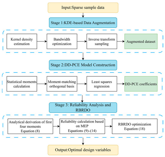
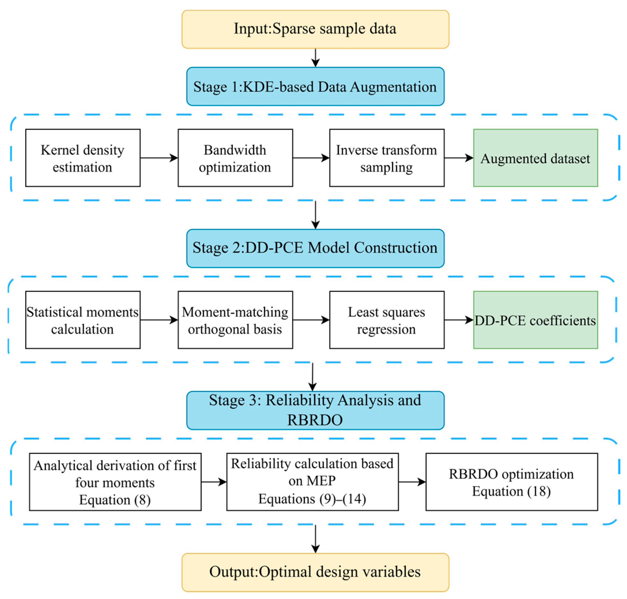
Figure 1 shows the processing flow of the distribution-unknown random variable RBRDO. For random variables with known distributions, their orthogonal polynomial basis functions are directly selected according to the Askey scheme based on the distribution type, without the need for KDE data augmentation.

Figure 1. RBRDO process for handling random variables with unknown distributions.

4. Numerical and Mechanical Structure Examples

In this section, the DD-PCE method is used to calculate the first four moments and reliability, and the results are compared with those obtained by MCS to verify the effectiveness of the DD-PCE method. First, the reliability of a two-stage worm gear reducer is analyzed as an example of a mechanical structure. Then, five numerical functions with different nonlinear characteristics are selected as test cases to further examine the applicability of the method in various complex situations.

4.1. Examples of Mechanical Structures

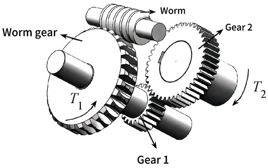
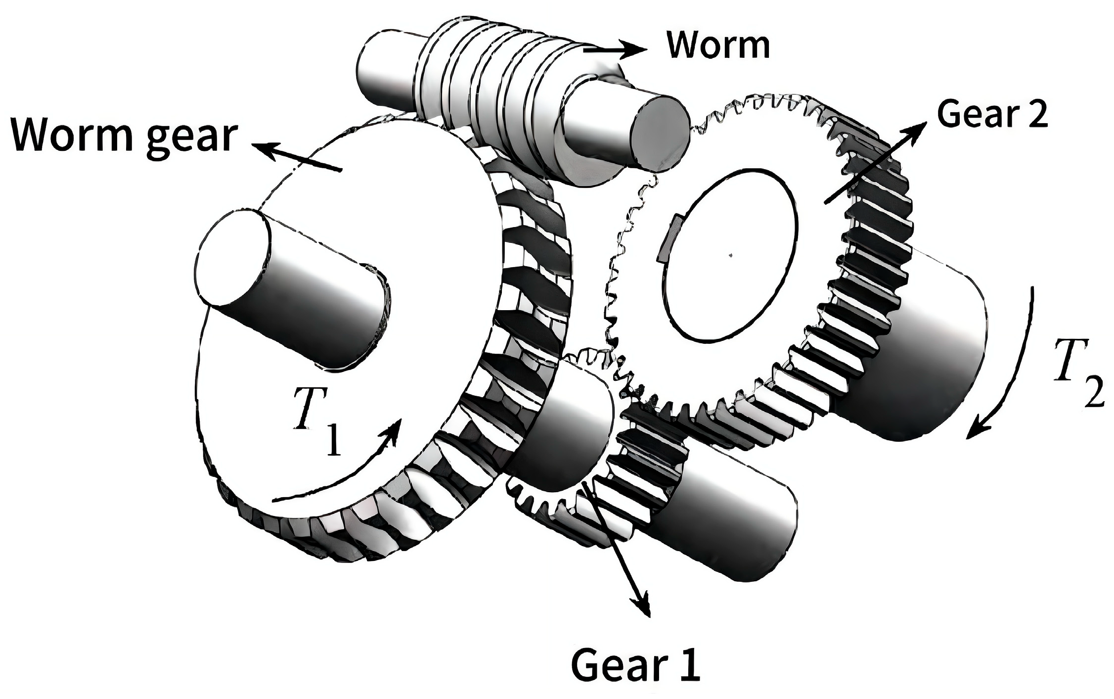
The two-stage worm gear reducer is an important mechanical transmission system characterized by high transmission efficiency, large reduction ratio, and compact structure. The two-stage worm gear reducer assembly is shown on Figure 2.

Figure 2. Assembly diagram of two-stage worm gear reducer.

The total reduction ratio of this reducer is i_t = 104. The first-stage worm gear transmission has a gear ratio of i₁ = 52, a module of m₁ = 8, a worm rotational speed of n₁ = 1440 r/min, a number of starts Z₁ = 1 for the worm, and a worm wheel tooth count Z₂ = 52. The second-stage gear transmission has a gear ratio of i₂ = 2, a module of m₂ = 12, Z₃ = 18 teeth for gear 1, Z₄ = 36 teeth for gear 2, and a tooth profile contact length of b = 42.

The worm gear and gears are critical components of this reducer, with their reliability being the primary factor influencing the overall reliability of the reducer. In worm gear transmissions, the worm typically does not fail due to the high strength of the commonly selected worm material. Furthermore, the failure modes of worm gear and gear transmissions are generally similar, including tooth surface wear, pitting, tooth contact fatigue failure, and tooth root bending fatigue fracture. Among these, tooth contact fatigue failure and tooth root bending fatigue fracture are the predominant failure modes. For simplicity, this study focuses on the tooth contact fatigue failure and tooth root bending fatigue failure of the worm wheel and the two transmission gears (gear 1 and gear 2), while neglecting failures in other components such as shafts, keys, and couplings.

The LSF for tooth contact fatigue failure of the worm gear is:

$$G_1=\left[{\sigma }_{\mathrm{H}1}\right]-Z_{\mathrm{E}1}\sqrt{{\displaystyle \frac{9K_1{T}_1}{d_1{d_2}^2}}}$$

(24)

where $[{\sigma }_{\mathrm{H}1}]$ represents the contact fatigue limit of the worm gear tooth surface, T₁ denotes the torque transmitted by the worm gear, K₁ is the load factor, Z_E1 stands for the elastic coefficient, while d₁ and d₂ are the pitch diameters of the worm and worm gear, respectively.

The LSF for bending fatigue fracture at the tooth root of the worm gear is:

$$G_2=\left[{\sigma }_{\mathrm{F}1}\right]-{\displaystyle \frac{1.53K_1{T}_1}{d_1{d}_2{m}_1}}{Y}_{\mathrm{Fa}}{Y}_{\gamma }$$

(25)

where $[{\sigma }_{\mathrm{F}1}]$ is the bending fatigue limit at the tooth root of the worm gear, Y_γ is the helix angle factor, Y_Fa is the tooth form factor.

The LSF for contact fatigue failure on the tooth surface of the gear is:

$$G_3=\left[{\sigma }_{\mathrm{H}2}\right]-Z_{\mathrm{E}2}{Z}_{\mathrm{H}}{Z}_{\epsilon }\sqrt{{\displaystyle \frac{2K_2{T}_2}{b{d}^2}}{\displaystyle \frac{u+1}{u}}}$$

(26)

where $[{\sigma }_{\mathrm{H}2}]$ represents the contact fatigue limit on the gear tooth surface, Z_H denotes the zone factor (meshing zone coefficient), Z_E2 is the material elastic coefficient, Z_ε is the contact ratio factor, T₂ indicates the torque transmitted by the gear, K₂ stands for the load factor, u is the gear ratio (teeth number ratio), b refers to the contact length between tooth profiles, and d is the reference circle diameter of the gear.

The LSF for bending fatigue fracture at the tooth root of the gear is:

$$G_4=\left[{\sigma }_{\mathrm{F}2}\right]-{\displaystyle \frac{2K_2{T}_2}{bd{m}_2}}{Y}_{\mathrm{F}}{Y}_{\mathrm{S}}{Y}_{\epsilon }$$

(27)

where $[{\sigma }_{\mathrm{F}2}]$ represents the bending fatigue limit at the tooth root of the gear, Y_ε is the contact ratio factor, Y_S denotes the stress correction factor, and Y_F is the tooth form factor.

The torques of the worm gear and the two gears involved in Equations (24)–(27) are derived from small sample sizes. Specifically, the torque values for the worm gear and gear 1 are as follows: (1,298,100, 1,298,000, 1,300,000, 1,297,000, 1,299,000, 1,296,000, 1,298,600, 1,298,190, 1,298,440, 1,298,690) N, while the torque values for gear 2 are (2,336,580, 2,336,570, 2,336,560, 2,336,550, 2,336,540, 2,336,530, 2,336,520, 2,336,510, 2,336,500, 2,336,480) N. To address the bias in statistical moment estimation resulting from the limited sample sizes, KDE is utilized to enhance the sparse data. This approach generates an augmented dataset comprising 10,000 data points through KDE.

All random variables are assumed to follow normal distributions. To avoid confusion between the parameters of the two gears, superscripts (i = 1, 2) are used to denote gear 1 and gear 2, respectively. The mean values and coefficients of variation (COV) for the worm gear are presented in Table 2, and those for the two gears are listed in Table 3.

Table 2. The mean values and COV of the random variables for the worm gear.

Variable	Mean	COV	Variable	Mean	COV
$[{\sigma }_{\mathrm{H}1}]$	550	0.05	ZE1	160	0.03
K1	1.15	0.033	$[{\sigma }_{\mathrm{F}1}]$	245	0.05
d1	8	0.015	YFa	2.5	0.033
d2	416	0.015	Yγ	0.92	0.033

Table 3. The mean values and COV of the random variables for the gears.

	Gear 1			Gear 2
Variable	Mean	COV	Variable	Mean	COV
$[{\sigma }_{\mathrm{H}2}^1]$	736	0.05	$[{\sigma }_{\mathrm{H}2}^2]$	550	0.03
$K_2^1$	1.15	0.033	$K_2^1$	1.15	0.033
b1	42	0.015	b2	42	0.015
d1	216	0.015	d2	432	0.015
${\mathrm{Z}}_{\mathrm{E}2}^1$	189.8	0.025	${\mathrm{Z}}_{\mathrm{E}2}^2$	189.5	0.025
${\mathrm{Z}}_{\mathrm{H}}^1$	2.5	0.033	${\mathrm{Z}}_{\mathrm{H}}^2$	2.5	0.033
${\mathrm{Z}}_{\epsilon }^1$	0.88	0.033	${\mathrm{Z}}_{\epsilon }^2$	0.88	0.033
$[{\sigma }_{\mathrm{F}}^1]$	220	0.05	$[{\sigma }_{\mathrm{F}}^2]$	136	0.05
$Y_{\mathrm{F}}^1$	2.42	0.033	$Y_{\mathrm{F}}^2$	2.28	0.033
$Y_{\mathrm{S}}^1$	1.68	0.04	$Y_{\mathrm{S}}^2$	1.77	0.04
$Y_{\epsilon }^1$	0.69	0.033	$Y_{\epsilon }^2$	0.69	0.033

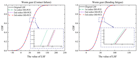
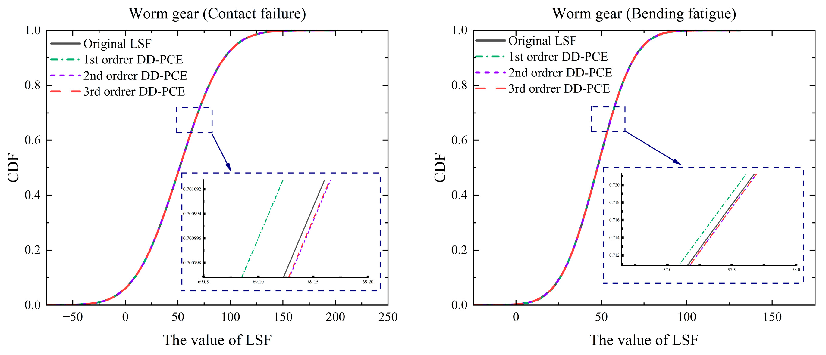
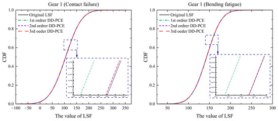
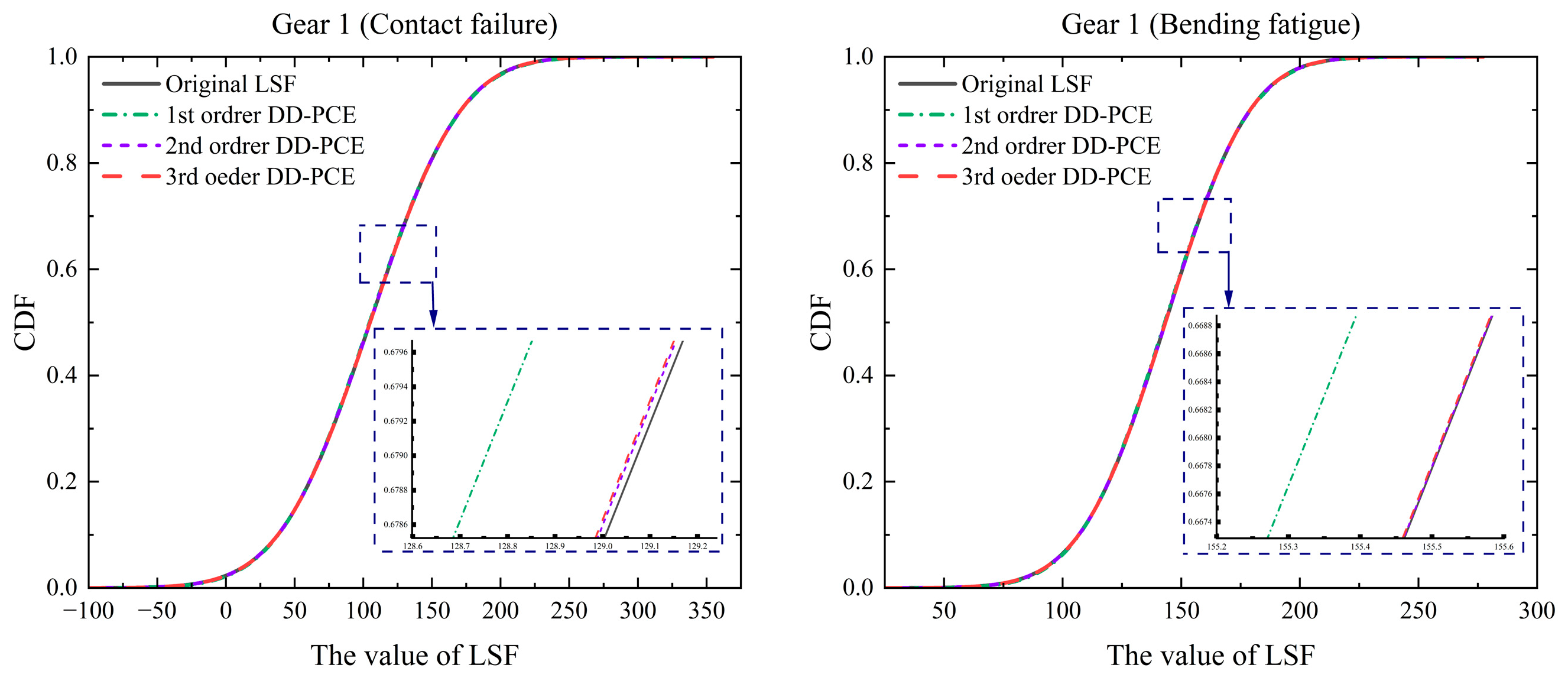
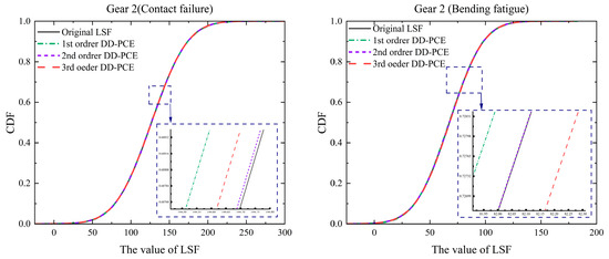
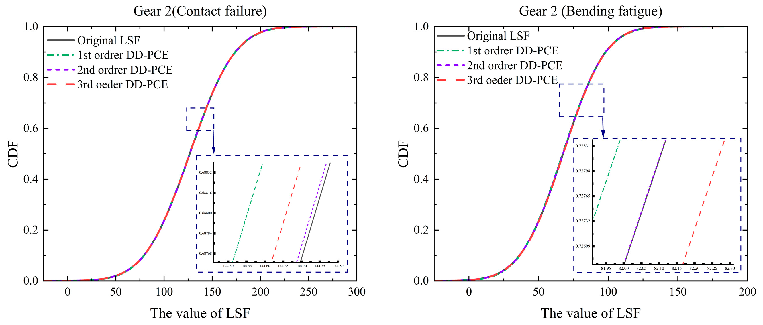
Based on the information provided in Table 2 and Table 3, the corresponding orthogonal polynomial bases were constructed. Subsequently, the coefficients of the DD-PCE were calculated using least squares regression. After substituting these coefficients into the DD-PCE model, the model for this LSF was established. In this study, to select an appropriate DD-PCE model, the CDFs of the 1st to 3rd DD-PCE models were compared with that of the original LSF. Figure 3, Figure 4 and Figure 5 present the comparative results for the worm gear, gear 1, and gear 2, respectively.

Figure 3. Comparison of CDF for Worm gear under two failure modes.

Figure 4. Comparison of CDF for Gear 1 under two failure modes.

Figure 5. Comparison of CDF for Gear 2 under two failure modes.

The results indicate that the CDFs of the first to third order DD-PCE models closely align with the original LSF. Notably, the computational accuracy of the second and third order models significantly surpasses that of the first order model. This discrepancy arises primarily because the first order model overlooks the impact of higher order terms. Theoretically, higher order DD-PCE models should yield improved computational accuracy. However, when precision requirements are met, these higher order models result in increased computational costs. Consequently, the third order DD-PCE model does not exhibit substantial advantages in this scenario, as its outcomes are nearly indistinguishable from those of the second order model. Therefore, the second order DD-PCE model was chosen for subsequent calculations.

To verify the accuracy of the model and assess the effectiveness of the KDE data augmentation method, a second-order DD-PCE model was constructed. The first four moments of the output response were analytically calculated using Equation (8) and compared with the results from 10⁶ MCS. Table 4 and Table 5 present the relative errors of the first four statistical moments compared to the MCS results when using KDE-enhanced data (10,000 points) and original sparse samples (10 points). In this context, e_μ, e_σ, e_β1 and e_β2 correspond to the relative errors of the first four moments. The comparison results indicate that after KDE enhancement, the maximum relative error of the first four moments across all failure modes is only 3.45%. In contrast, using the original sparse samples directly results in an error of up to 214.70%. This significant difference demonstrates that the KDE data augmentation method effectively alleviates the statistical moment estimation bias caused by sparse samples, thereby improving the accuracy of reliability analysis. Furthermore, the reliability was calculated using the maximum entropy method and compared with the 10⁶ MCS, as shown in Table 6. Here, R_DD-PCE and R_MCS represent the reliability calculated using the proposed method and the MCS method, respectively, while e_R denotes the relative error of the reliability. From Table 6, it is evident that the relative error in reliability between the DD-PCE calculated using the maximum entropy method and the maximum reliability calculated by MCS is 0.37%. Notably, the computation time for the proposed method is less than 5% of that required for MCS, which fully demonstrates that the proposed method achieves both high accuracy and significant computational efficiency.

Table 4. Relative errors of the first four moments after KDE augmentation.

Parts	Failure Mode	MCS	eμ (%)	eσ (%)	eβ1 (%)	eβ2 (%)
Worm gear	Contact failure	-	0.87	1.51	3.12	3.45
	Bending fatigue	-	0.25	1.05	1.93	2.22
Gear 1	Contact failure	-	0.29	1.01	2.66	0.84
	Bending fatigue	-	0.12	1.75	1.51	1.54
Gear 2	Contact failure	-	0.21	1.12	3.11	0.77
	Bending fatigue	-	0.14	1.73	3.14	3.39

Table 5. Relative errors of the first four moments for the original samples.

Parts	Failure Mode	MCS	eμ (%)	eσ (%)	eβ1 (%)	eβ2 (%)
Worm gear	Contact failure	-	7.593	11.75	38.91	18.758
	Bending fatigue	-	2.773	8.99	55.01	26.309
Gear 1	Contact failure	-	6.909	10.80	147.91	11.079
	Bending fatigue	-	8.820	9.135	188.69	18.139
Gear 2	Contact failure	-	5.221	10.46	214.70	8.875
	Bending fatigue	-	9.542	13.183	107.46	6.361

Table 6. Comparison of reliability calculation results across different failure modes.

Parts	Failure Mode	RDD-PCE	Time/s	RMCS	Time/s	eR
Worm gear	Contact failure	0.9421	0.465	0.9386	18.35	0.37%
	Bending fatigue	0.9969	0.47	0.9969	19.25	0%
Gear 1	Contact failure	0.9781	0.445	0.9769	18.49	0.12%
	Bending fatigue	1.0	0.577	1.0	18.86	0%
Gear 2	Contact failure	0.9997	0.413	0.9996	18.41	0.01%
	Bending fatigue	0.9975	0.507	0.9966	18.59	0.09%

4.2. Numerical Examples

To systematically evaluate the performance of the proposed method in terms of accuracy and computational efficiency, this section tests five mathematical functions characterized by varying levels of nonlinearity and dimensions. The specific forms of these functions are presented in Table 7. In the table, N, U, and Rayl denote random variables that follow a normal distribution, uniform distribution, and Rayleigh distribution, respectively, while BM represents random variables that follow a bimodal distribution, defined by its PDF in Equation (28). It is important to note that in practical engineering applications, the specific forms of these distributions are often unknown, and only limited sample data are available. As discussed in Section 4.1, the high-order PCE model does not exhibit significant advantages for such problems; therefore, the PCE order for all functions is set to 2.

$$f_{\mathrm{PDF}}={\displaystyle \frac{0.647}{0.1\sqrt{2\pi }}}\exp \left(-{\displaystyle \frac{x^2}{2\times {0.1}^2}}\right)+{\displaystyle \frac{0.353}{0.2\sqrt{2\pi }}}\exp \left(-{\displaystyle \frac{{\left(x-1\right)}^2}{2\times {0.2}^2}}\right) x\in \left[-\infty ,+\infty \right]$$

(28)

Table 7. Test functions and random input information.

Function 1: $y=x_1+x_2-x_3$ 500 and 104 sample points $x_1\sim BM,x_2\sim BM,x_3\sim N\left(-0.8,0.2\right)$ Function 2: $y=\sin \left(x_1\right)-{\cos }^2\left(x_2\right)+x_3\sin \left(x_1\right)+0.9$ 500 and 104 sample points $x_1\sim BM,x_2\sim BM,x_3\sim U\left(0.4,2\right)$ Function 3: $y=e^{-x_1}\cos \left(x_2\right)+x_3{e}^{-\left(x_4{x}_5\right)}-e^{-x_6}$ 500 and 104 sample point $x_1\sim BM,x_2\sim Rayl\left(0.3\right),x_3\sim BM,x_4\sim Rayl\left(0.3\right),x_5\sim BM,x_6\sim Rayl\left(1\right)$ Function 4: $y=x_1^2{x}_2^2-x_3^2{x}_4^2+x_5^2{x}_6^2-x_7^2{x}_8^2+x_9^2{x}_{10}^2$ 500 and 104 sample points $x_1\sim N\left(1.5,0.2\right),x_2\sim N\left(1,0.2\right),x_3\sim BM,x_4\sim BM,x_5\sim N\left(1,0.2\right)$ $x_6\sim N\left(1,0.2\right),x_7\sim N\left(0,0.2\right),x_8\sim N\left(0,0.2\right),x_9\sim N\left(1,0.2\right),x_{10}\sim N\left(1,0.2\right)$ Function 5: $y=e^{x_1\sin \left(x_2\right)}+\log \left(1+x_3^2{x}_4^2\right)-\cos \left(x_5{e}^{x_6}\right)$ 500 and 104 sample point $x_1\sim BM,x_2\sim N\left(0,0.5\right),x_3\sim BM,x_4\sim U\left(0.5,1.5\right),x_5\sim Rayl\left(0.3\right),x_6\sim U\left(0,1\right)$

To examine the impact of the number of input variable samples on statistical moment estimation, tests were conducted using both a small sample size (500) and a large sample size (10⁴) as inputs. From Table 8, Table 9, Table 10, Table 11, Table 12, it is evident that when the number of input variable sampling points is large (10⁴), the results of the DD-PCE calculations closely align with those obtained from MCS. Conversely, when the number of sampling points is 500, the error significantly increases. This finding indicates that as the number of input variable samples increases, the estimation accuracy of DD-PCE is markedly enhanced. The underlying principle is that with a greater number of sampling points, the statistical moments of the random input variables are calculated with improved accuracy. It is important to note that the computational cost of the DD-PCE method, specifically the number of function evaluations, is equal to the required sample size (500 or 10⁴ evaluations).

Table 8. Relative error results of Function 1.

Methods	MCS (107)	DD-PCE (500)	DD-PCE (104)
eμ (%)	-	1.8951	0.0348
eσ (%)	-	1.8225	0.0520
eβ1 (%)	-	6.4570	1.0456
eβ2 (%)	-	10.8254	0.4377
Pf (1 × 10−4)	[2.12, 2.30]	0	2.16

Table 9. Relative error results of Function 2.

Methods	MCS (107)	DD-PCE (500)	DD-PCE (104)
eμ (%)	-	3.5082	0.4687
eβ1 (%)	-	0.7094	0.2806
eβ2 (%)	-	0.4141	1.2179
eβ2 (%)	-	1.5878	2.2330
Pf	[0.2828, 0.2834]	0.284	0.2831

Table 10. Relative error results of Function 3.

Methods	MCS (107)	DD-PCE (500)	DD-PCE (104)
eμ (%)	-	3.5697	0.3873
eβ1 (%)	-	1.3981	0.3816
eβ2 (%)	-	27.3714	1.8397
eβ2 (%)	-	11.340	1.6012
Pf	[0.1134, 0.1138]	0.12	0.1179

Table 11. Relative error results of Function 4.

Methods	MCS (107)	DD-PCE (500)	DD-PCE (104)
eμ (%)	-	1.0002	0.0723
eβ1 (%)	-	1.9386	0.9712
eβ2 (%)	-	7.0708	1.7387
eβ2 (%)	-	19.0758	6.4824
Pf (1 × 10−4)	[8.04, 8.39]	0	8.25

Table 12. Relative error results of Function 5.

Methods	MCS (107)	DD-PCE (500)	DD-PCE (104)
eμ (%)	-	2.6508	0.1299
eβ1 (%)	-	2.0392	0.9401
eβ2 (%)	-	34.2277	14.1454
eβ2 (%)	-	26.7463	9.6618
Pf (1 × 10−2)	[6.174, 6.204]	8.516	7.161

From Table 8, Table 9, Table 10, Table 11 and Table 12, it can be observed that the DD-PCE method exhibits significant performance differences when addressing functions with varying degrees of nonlinearity. For linear functions (Function 1) and moderately nonlinear functions (Functions 2 and 4), when the sample size reaches 10⁴, the failure probability estimated by DD-PCE falls within the 95% confidence interval of MCS. However, for strongly nonlinear functions (Functions 3 and 5), even with 10⁴ samples, the failure probability estimated by DD-PCE still exceeds the 95% confidence interval of MCS. This result indicates that when the LSF demonstrates strong nonlinear characteristics, the second-order PCE model fundamentally struggles to accurately approximate the statistical properties of complex nonlinear responses. Furthermore, a comparison between the results of 500 samples and 10⁴ samples reveals that with an insufficient number of samples, the errors in skewness and kurtosis for all functions significantly increase, leading to failure probability estimates of 0 for Function 1 and Function 4, which completely deviate from the true values. This further illustrates that the DD-PCE method is highly sensitive to the number of input samples, and substantial deviations may occur under extremely sparse sample conditions.

5. Engineering Case Studies

This section presents three examples of structural analysis and one engineering case study to demonstrate the applicability and robustness of the proposed RBRDO methodology. The first example involves the analysis of a cantilever hollow tube, the second focuses on a simply supported beam structure, and the third examines a cantilever beam. Additionally, the fourth case study analyzes the primary steel spring of a fast metro vehicle. For all four structural cases, surrogate models are constructed using the second-order DD-PCE model.

5.1. Example 1: Cantilever Hollow Tube

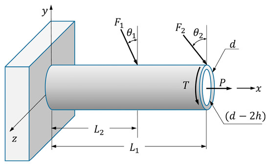
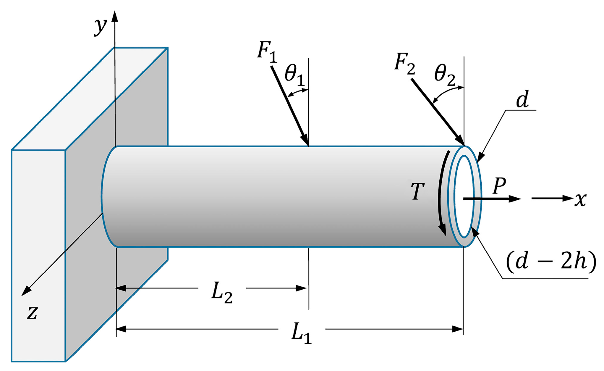
As shown in Figure 6, the cantilever tube is subjected to two inclined transverse forces, F₁ and F₂, which act at the midpoint and the end of the cantilever tube, respectively. The loading angles of these forces in the vertical direction are denoted as θ₁ and θ₂, with the corresponding load positions labeled as L₁ and L₂ [50]. Additionally, a torque T is applied at the end of the cantilever tube, while an axial load P is also applied along its length. The parameters d and h represent the outer diameter and wall thickness of the cantilever tube, respectively. In this context, the distribution types of F₁, F₂, P, and T remain unknown, with only limited samples available, as shown in Table 13. KDE was employed to generate 10,000 data points for each small sample, while the remaining random variables are assumed to be mutually uncorrelated, as indicated in Table 14.

Figure 6. Cantilevered hollow tube.

Table 13. Sample data for an unknown distribution of cantilever hollow tubes.

Variable	Samples
F1 (N)	12,100, 11,990, 11,999, 12,010, 11,100, 12,000, 12,046, 13,076, 12,554, 12,073
F2 (N)	12,200, 12,990, 11,849, 11,910, 12,009, 12,035, 12,170, 12,076, 13,044, 11,973
P (N)	14,900, 15,000, 15,305, 15,200, 14,700, 14,060, 15,050, 15,140, 14,980, 15,080
T (N)	80,150, 80,400, 80,350, 80,010, 80,000, 80,093, 80,041, 80,145, 79,800, 79,950

Table 14. Probabilistic properties of random variables for the cantilever hollow tube.

Variable	Distribution	Mean (* Lower Bound)	Standard Deviation (** Upper Bound)	Unit
h	Normal	6	0.06	mm
d	Normal	50	0.5	mm
L1	Uniform	120 *	125 **	mm
L2	Uniform	60 *	65 **	mm
S	Normal	400	40	MPa
θ1	Normal	π/18	π/180	rad
θ2	Normal	π/36	π/360	rad

The LSF can be defined in terms of the yield strength S and maximum von Mises stress ${\sigma }_{\max }$ in the circumferential surface of the clamped end of the cantilever tube, given as,

$$g=S-{\sigma }_{\max }$$

(29)

The cantilever tube will fail if ${\sigma }_{\max }$ exceeds the yield strength S. In this case, von Mises stress ${\sigma }_{\max }$ can be expressed as

$${\sigma }_{\max }=\sqrt{{\sigma }_x^2+3{\tau }_{xz}^2}$$

(30)

where the equations for determining ${\sigma }_{\max }$ can be derived by

$${\sigma }_x={\displaystyle \frac{P+F_2\sin {\theta }_2+F_1\sin {\theta }_1}{A}}+{\displaystyle \frac{Mc}{I}}$$

(31)

$$M=(F_2{L}_1\cos {\theta }_2+F_1{L}_2\cos {\theta }_1)$$

(32)

$$A={\displaystyle \frac{\pi }{4}}[d^2-{\left(d-2h\right)}^2]$$

(33)

$$c={\displaystyle \frac{d}{2}}$$

(34)

$$I={\displaystyle \frac{\pi }{64}}[d^4-{\left(d-2h\right)}^4]$$

(35)

$${\tau }_{xz}={\displaystyle \frac{16dT}{\pi [d^4-{\left(d-2h\right)}^4]}}$$

(36)

where A is the area of the end section of the cantilever tube, ${\tau }_{xz}$ is the shear stress, ${\sigma }_x$ is the superimposed normal stress in the x-axis direction.

The RBRDO method utilizes the thickness h and diameter d of the cantilever tube as design variables. It imposes constraints that the thickness must be no less than 5 mm and no greater than 8 mm, and the diameter must be no less than 48 mm and no greater than 55 mm. This approach allows for the optimization of the structural parameters of the cantilever tube while adhering to reliability requirements. The established model is as follows:

$$\begin{array}{l}\underset{h,d}{\min } w_1{l}_1+w_2{l}_2\\ \mathrm{st}: R_{\mathrm{DD}\text{-}\mathrm{PCE}}\ge R_0\\ \mathrm{Design} \mathrm{variables}: 5 \mathrm{mm}\le h\le 8 \mathrm{mm};\\ 48 \mathrm{mm}\le d\le 55 \mathrm{mm}\end{array}$$

(37)

where the initial values for h and d are set to h = 6 mm and d = 50 mm, respectively. Here, R₀ denotes the specified reliability requirement, defined as 0.999. Furthermore, the objective function of the RBRDO is the cross-sectional area f of the cantilevered hollow tube, expressed as follows:

$$f={\displaystyle \frac{\pi }{4}}\left[d^2-{\left(d-2h\right)}^2\right]$$

(38)

Table 15 presents the results of the cantilever hollow tube before and after robust optimization.

Table 15. RBRDO results of the cantilevered hollow tube.

	Design Variables	RDD-PCE	Time/s	RMCS	Time/s	eR
Pre-design	[h, d]T = [6, 50]T	0.9964	0.995	0.9959	19.54	0.05%
Post-design	[h, d]T = [6.3, 51.2]T	0.9997	0.847	0.9995	19.39	0.02%

From Table 15, after robust optimization, the reliability improved from 0.9964 to 0.9997, meeting the target requirement R₀ = 0.999. The relative error between DD-PCE and MCS is only 0.05%, while the computation time is reduced by approximately 95%.

5.2. Example 2: Simply Supported Beam

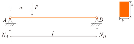
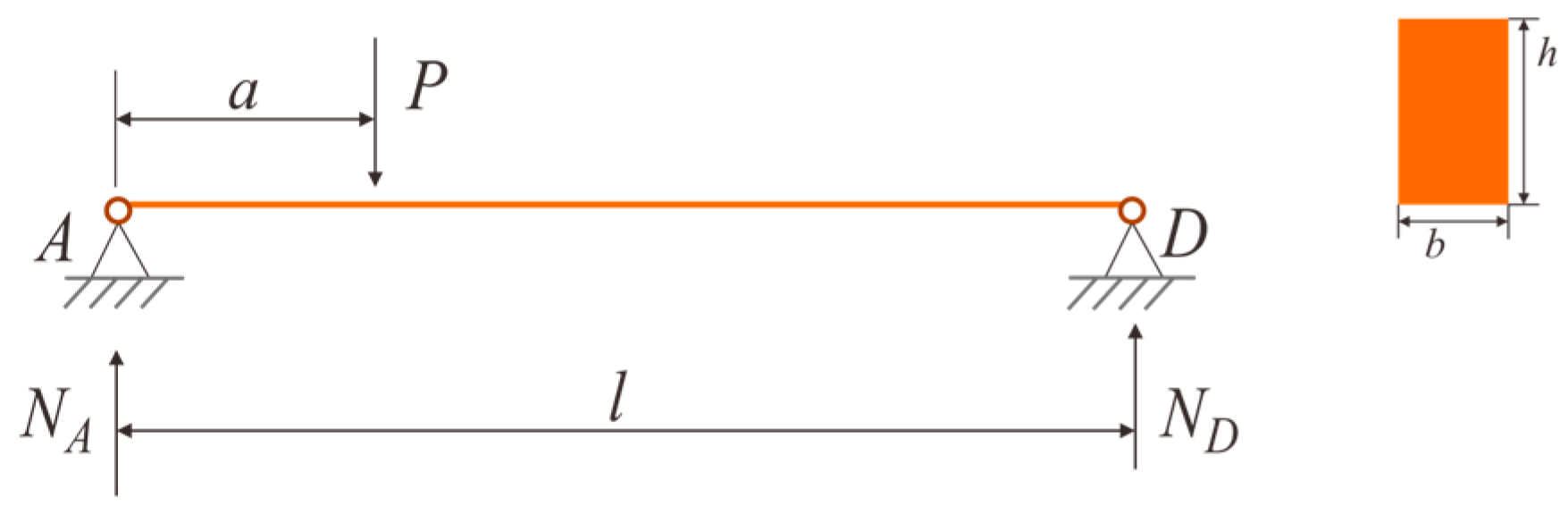
The simply supported beam is shown in Figure 7. Since the primary failure mode of the beam is the excessive bending stress caused by the bending moment, only this condition is considered [51].

Figure 7. Simply supported beam.

A simply supported beam is subjected to a concentrated force P. The self-weight of the beam is neglected. The span of the beam is l, the distance from the concentrated force to fixed support A is a, and the cross-sectional dimensions of the beam are height h and width b. l, a, h, and b are all random variables following a normal distribution. Among these, the distribution type of the concentrated load P is unknown with only a small number of samples available, The sample is (17,400, 12,600, 18,000, 18,300, 16,300, 17,000, 14,000, 17,200, 20,200, 19,000) N, use KDE to generate 10,000 data points for load P. The remaining random variables are assumed to be mutually uncorrelated, as detailed in Table 16.

Table 16. Distribution details of random variables.

Variable	Distribution	Mean	Standard Deviation	Unit
S	Normal	500	50	MPa
l	Normal	3000	10	mm
a	Normal	1200	10	mm
b	Normal	35	0.19	mm
h	Normal	76	0.39	mm

The LSF can be defined by:

$$g=S-{\sigma }_{\max }$$

(39)

According to the mechanics of materials, the functional relationship between the maximum stress a beam is subjected to, and its cross-sectional dimensions is given by:

$${\sigma }_{\max }={\displaystyle \frac{Mh/2}{b{h}^3/12}}$$

(40)

where the maximum bending moment $M={\displaystyle \frac{Pa(1-a)}{l}}$.

The RBRDO method employs the width b and height h of a simply supported beam as design variables, constrained such that the width is at least 30 mm and at most 50 mm, while the height is constrained to be no less than 60 mm and no greater than 80 mm. This methodology allows for the optimization of the beam’s structural parameters while ensuring compliance with reliability requirements. The established model is as follows:

$$\begin{array}{l}\underset{b,h}{\min } w_1{l}_1+w_2{l}_2\\ \mathrm{st}: R_{\mathrm{DD}\text{-}\mathrm{PCE}}\ge R_0\\ \mathrm{Design} \mathrm{variables}: 30 \mathrm{mm}\le b\le 50 \mathrm{mm};\\ 60 \mathrm{mm}\le h\le 80 \mathrm{mm}\end{array}$$

(41)

where the initial values for b and h are set to b = 35 mm and h = 76 mm, respectively. Here, R₀ denotes the specified reliability requirement, which is defined as 0.999. Furthermore, the objective function of the RBRDO is the cross-sectional area f, expressed as follows:

$$f=bh$$

(42)

Table 17 lists the design results before and after the robust optimization of the simply supported beam.

Table 17. RBRDO results for simply supported beams.

	Design Variables	RDD-PCE	Time/s	RMCS	Time/s	eR
Pre-design	[b, h]T = [35, 76]T	0.9951	0.862	0.9954	20.29	0.03%
Post-design	[b, h]T = [39.5, 77]T	0.9998	0.811	0.9997	19.35	0.01%

From Table 17, the optimized design achieves a reliability of 0.9998, satisfying the prescribed requirement R₀ = 0.999. The DD-PCE method shows excellent agreement with MCS (relative error 0.03%) while requiring only about 4% of the MCS computation time.

5.3. Example 3: Cantilever Beam Structure

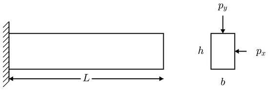
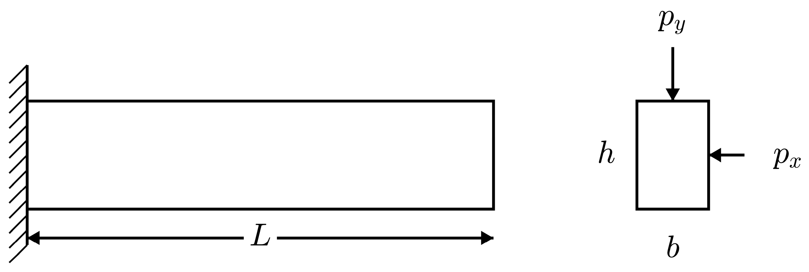
This section employs a cantilever beam structure [36], as illustrated in Figure 8. In this context, the geometric parameters primarily encompass the total length of the beam L, the cross-sectional width b, and the height of the beam h. The loading conditions on the beam are characterized by two primary forces, denoted as p_x and p_y. To ensure structural reliability, the permissible stress for the material performance parameter is established at S = 350 MPa. The distribution types of loads p_x and p_y are unknown, with only a small number of samples available. The sample values are as follows: (50,018, 49,996, 50,026, 49,999, 50,012, 50,027, 50,035, 49,984, 49,949, 50,019) N for p_x and (24,972, 25,002, 25,027, 24,961, 25,024, 25,026, 24,979, 25,031, 25,006, 24,995) N for p_y. A total of 10,000 data points is generated using KDE. The remaining random variables are assumed to be independent, as detailed in Table 18.

Figure 8. Cantilever beam structure.

Table 18. RBRDO results for cantilever beam structure.

Variable	Distribution	Mean	Standard Deviation	Unit
L	Normal	1000	100	mm
b	Normal	100	10	mm
h	Normal	200	20	mm

The LSF can be defined by:

$$g=S-{\sigma }_{\max }$$

(43)

${\sigma }_{\max }$ is defined by the following equation:

$${\sigma }_{\max }={\displaystyle \frac{6p_{x}L}{b^{2}h}}+{\displaystyle \frac{6p_{y}L}{b{h}^2}}$$

(44)

The RBRDO method utilizes the width b and height h of the cantilever beam as design variables. The constraints dictate that the width must not be less than 80 mm and not exceed 130 mm, while the height must be no less than 160 mm and no greater than 240 mm. This method facilitates the optimization of the cantilever beam’s structural parameters while ensuring compliance with the reliability requirements. The established model is articulated as follows:

$$\begin{array}{l}\underset{b,h}{\min } w_1{l}_1+w_2{l}_2\\ \mathrm{st}: R_{\mathrm{DD}\text{-}\mathrm{PCE}}\ge R_0\\ \mathrm{Design} \mathrm{variables}: 80 \mathrm{mm}\le b\le 130 \mathrm{mm};\\ 160 \mathrm{mm}\le h\le 240 \mathrm{mm}\end{array}$$

(45)

where the initial values for b and h are set at b = 100 mm and h = 200 mm; R₀ denotes the specified reliability requirement, defined as 0.999. Furthermore, the objective function of the RBRDO method is the cross-sectional area f, expressed as follows:

$$f=bh$$

(46)

Table 19 lists the design results before and after the robust optimization of the cantilever beam.

Table 19. RBRDO results for cantilever beam.

	Design Variables	RDD-PCE	Time/s	RMCS	Time/s	eR
Pre-design	[b, h]T = [100, 200]T	0.8548	0.985 s	0.8607	19.39 s	0.6%
Post-design	[b, h]T = [120, 180]T	0.9999	0.967 s	0.9998	20.42 s	0.02%

From Table 19, it can be seen that the optimized design achieves a reliability of 0.9999, meeting the prescribed reliability requirement R₀ = 0.999. The DD-PCE method shows excellent agreement with MCS (maximum relative error of 0.6%) while requiring less than 5% of the MCS computation time.

5.4. Example 4: Primary Steel Spring of the Fast Metro Vehicle

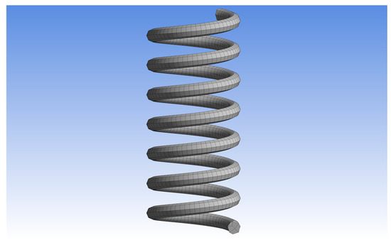
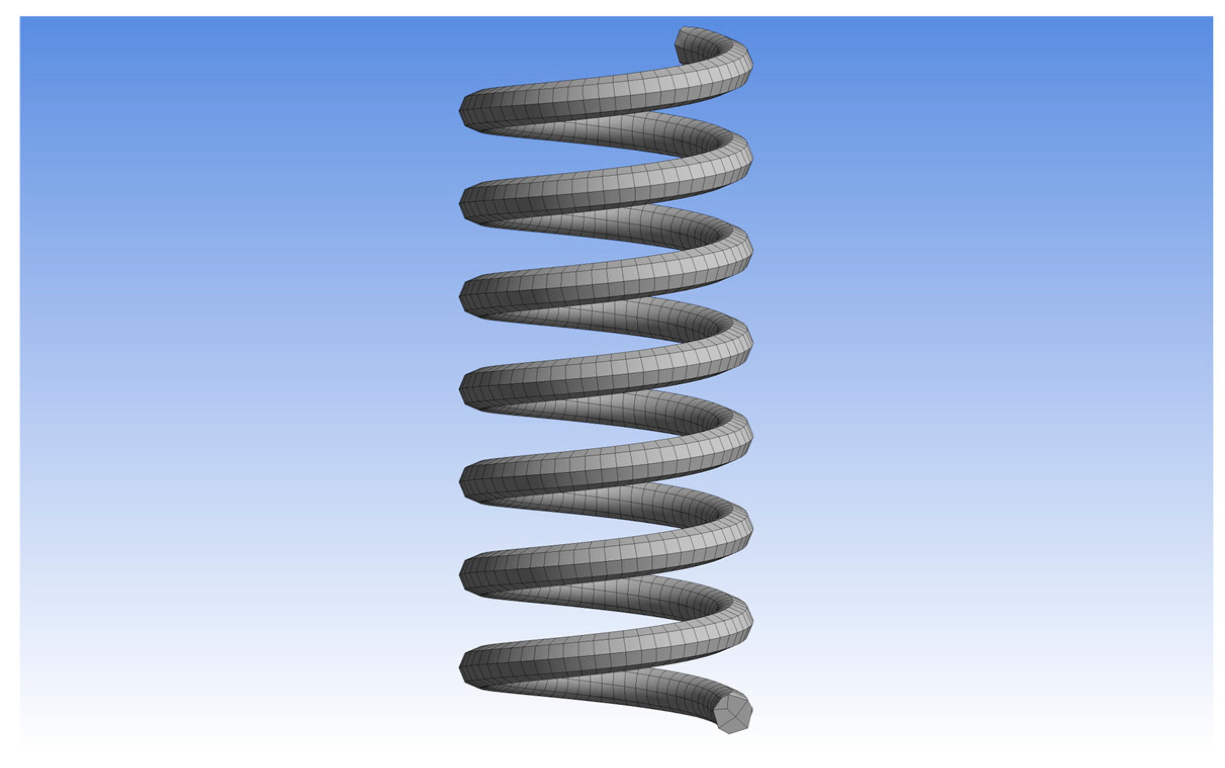
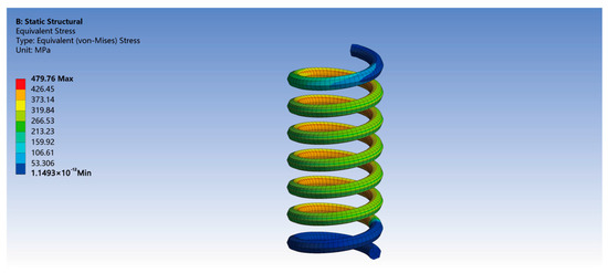
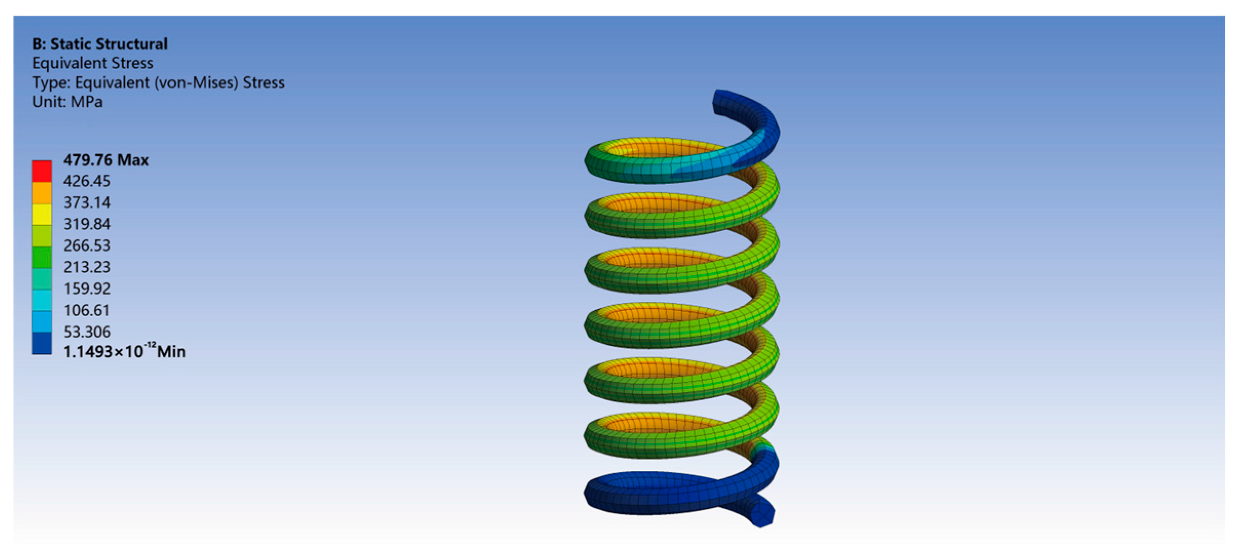
To further demonstrate the effectiveness of the proposed method in practical engineering applications, this paper conducts a reliability robust design for the primary steel spring of the fast metro vehicle, as illustrated in its three-dimensional model in Figure 9. A finite element simulation (FES) was performed in the spring, with the corresponding simulation results presented in Figure 10. The steel spring of the fast metro vehicle is fabricated from 51CrV4 steel, and its fundamental material properties are listed in Table 20. Here, E denotes the modulus of elasticity, v represents Poisson’s ratio, ρ indicates the density, and G signifies the shear modulus.

Figure 9. Three-dimensional model of the spring.

Figure 10. Stress analysis results of the spring.

Table 20. Material properties of 51CrV4 steel.

Parameter	Numerical Value
S (MPa)	1127.00
E (GPa)	206.00
G (GPa)	78.50
v	0.30
ρ (kg/m3)	7800

This study primarily focuses on conducting a reliability analysis of stress while considering structural dimensional uncertainties in steel springs. The inherent geometrical parameters of springs significantly affect their stiffness and load-bearing capacity, with uncertainties propagating into critical dimensions such as the diameter of the spring wire, the middle diameter of the spring, and the number of effective coils. These parameters can introduce uncertainty in stress, thereby impacting the reliability of the spring. To address this issue, the method proposed in this paper is utilized to perform RBRDO analysis on the spring, with its LSF presented as follows.

$$y(\mathit{x})=S-{\sigma }_{\max }(r_1,r_2,N,F)$$

(47)

where ${\sigma }_{\max }$ denotes the maximum stress derived from the FES of the spring, while S represents the yield strength of the material. The vector of uncertain random variables, denoted as x = [r₁, r₂, N, F], comprises the wire diameter r₁, the middle diameter r₂, the effective number of coils N, and the load F of the spring. Load F does not have a known distribution type and is represented by a limited number of samples. The sample values are (5100, 5090, 4999, 5010, 5009, 5035, 5046, 5076, 5054, 5073) N. KDE is employed to generate 10,000 data points for load F. The detailed statistical information of the aforementioned random variables is presented in Table 21.

Table 21. The relevant information of random variables.

Variable	Distribution	Mean	Standard Deviation
r1	Normal	21.75	0.15
r2	Normal	135.8	0.2
N	Normal	7.14	0.1

The RBRDO methodology identifies the spring wire diameter, middle diameter, and number of active coils as design variables. The design must adhere to the following specifications: the wire diameter should be no less than 20 mm and no greater than 24 mm, the middle diameter must range from 125 mm to 145 mm, and the number of effective coils must be between 5 and 9. This approach facilitates the optimization of structural parameters while ensuring compliance with established reliability requirements. The formulated mathematical model is expressed as follows:

$$\begin{array}{l}\underset{r_1,r_2,N}{\min } w_1{l}_1+w_2{l}_2\\ \mathrm{st}: R_{\mathrm{DD}\text{-}\mathrm{PCE}}\ge R_0\\ \mathrm{Design} \mathrm{variables}: 20 \mathrm{mm}\le r_1\le 24 \mathrm{mm};\\ 125 \mathrm{mm}\le r_2\le 145 \mathrm{mm};\\ 5\le N\le 9\end{array}$$

(48)

where the design variables are initialized with the following values: r₁ = 21.75, r₂ = 135.8, N = 7.14. R₀ represents the specified reliability requirement, defined as R₀ = 0.999. The RBRDO methodology defines the spring volume as the objective function, mathematically expressed as:

$$f={\displaystyle \frac{\pi }{4}}\cdot r_1^2\cdot r_2\cdot N$$

(49)

Table 22 lists the design results of the spring before and after robust optimization.

Table 22. RBRDO results for springs.

	Design Variables	RDD-PCE	Time/s	RMCS	Time/s	eR
Pre-design	[r1, r2, N]T = [21.75, 135.8, 7.14]T	0.9981	0.943	0.9980	19.75	0.01%
Post-design	[r1, r2, N]T = [21.72, 135.98, 7.16]T	0.9996	0.924	0.9997	18.92	0.01%

The comparison results presented in Table 22 indicate that the reliability of the structure increased from 0.9981 to 0.9996 following robust optimization, thereby satisfying the reliability requirement of 0.999. Furthermore, the relative error between the DD-PCE method and the MCS method in the calculation results, both before and after robust optimization, is only 0.01%, which demonstrates the high numerical accuracy of the proposed method. Additionally, the computation time of the DD-PCE method is less than 5% that of the MCS method, further substantiating its superiority in computational efficiency.

5.5. Example Analysis Summary

The results presented in Table 15, Table 17 and Table 19, and 22 indicate that prior to robust optimization for the cantilever hollow tube, simply supported beam, cantilever beam, and spring, the relative errors in reliability between the DD-PCE method and the MCS method were 0.05%, 0.03%, 0.6%, and 0.01%, respectively. The corresponding calculation times accounted for 5.1%, 4.2%, 5.1%, and 4.8% of the MCS times. Following robust optimization, the optimized results were utilized to determine reliability using both the DD-PCE and MCS methods. Post-optimization, the reliability improved to the 0.999 level, with relative errors of 0.02%, 0.01%, 0.02%, and 0.01%, while the calculation times reduced to only 4.4%, 4.2%, 4.7%, and 5% of the MCS times. In summary, compared to the traditional MCS method, the DD-PCE method exhibits significant advantages in both computational accuracy and efficiency, substantially decreasing computation time while preserving high precision.

6. Conclusions

This study addresses the issues of poor reliability and insufficient computational efficiency caused by incomplete information about random variables and sparse sampling in practical engineering scenarios. A DD-PCE model tailored for scenarios with limited samples was proposed and applied to RBRDO. The DD-PCE method constructs orthogonal polynomial basis functions directly from input data through moment matching and determines coefficients via regression. To enhance accuracy further, data augmentation using KDE was performed, alleviating the statistical moment bias associated with sparse sampling. After obtaining the DD-PCE model, the first four statistical moments of the output response were derived analytically, and reliability was efficiently calculated based on the MEP, thus avoiding the additional step of calculating reliability typically required by traditional PCE methods. In the case analysis of a two-stage worm gear reducer, the appropriate DD-PCE model was selected by comparing the CDFs of the first to third order DD-PCE models with the original LSF. The comparison demonstrated that the CDF of the second-order model closely matched the original LSF. To verify the effectiveness of KDE-based data augmentation, we compared the computational results of KDE-augmented data (10,000 points) with those of the original samples (10 points). After KDE augmentation, the maximum relative error of the first four moments was only 3.45%, whereas directly using the original samples resulted in an error as high as 214.70%. This clearly demonstrates that the KDE method effectively mitigates the bias in statistical moment estimation caused by sparse samples. Furthermore, based on the maximum entropy approach, the reliability of contact fatigue and bending fatigue was calculated and compared with MCS results, yielding a maximum relative error of 0.37%, while the computation time was less than 5% of that required by MCS, significantly improving computational efficiency. The proposed method was further validated using five mathematical functions with varying degrees of nonlinearity. The results showed that when the sample size reached 10⁴, the DD-PCE method estimated the failure probability of linear and moderately nonlinear functions within the 95% confidence interval of MCS; however, for strongly nonlinear functions, the second-order PCE model struggled to accurately approximate the statistical characteristics of the complex nonlinear response. Further integration of DD-PCE and L-moments into the RBRDO framework achieved parameter optimization for the cantilever hollow tube, simply supported beam, cantilever beam, and primary steel spring of the fast metro vehicle. The reliability enhanced through robustness improvements reached a level of 0.999, while the maximum computational time was only 5.1% of that required by the MCS method, demonstrating exceptional computational efficiency. This research addresses the traditional PCE method’s reliance on complete statistical information, offering a novel technological pathway for high-reliability design in contexts where data for complex equipment is limited, thus holding significant engineering application value.

References

- Zhao, J.; Guo, J.; Wang, J.; Xu, H. An Improved High-Moment Method for Reliability Analysis Based on Polynomial Chaos Expansion. IOP Conf. Ser. Mater. Sci. Eng. 2021, 1043, 032002. [Google Scholar] [CrossRef] [Scilit]
- Guo, H.; Luo, C.; Zhu, S.-P.; You, X.; Yan, M.; Liu, X. Machine Learning-Based Enhanced Monte Carlo Simulation for Low Failure Probability Structural Reliability Analysis. Structures 2025, 74, 108530. [Google Scholar] [CrossRef] [Scilit]
- Huang, W.B.; Mao, J.G.; Zhang, Z.Y. The Maximum Entropy Estimation of Structural Reliability Based on Monte Carlo Simulation. In Proceedings of the ASME 2014 33rd International Conference on Ocean, Offshore and Arctic Engineering, San Francisco, CA, USA, 8–13 June 2014. [Google Scholar] [CrossRef] [Scilit]
- Zhao, Y.-G.; Ono, T. Moment Methods for Structural Reliability. Struct. Saf. 2001, 23, 47–75. [Google Scholar] [CrossRef] [Scilit]
- Liu, X.; Deng, J.; Chen, H.; Zhai, G.; Wu, J. An Efficient and Multi-Fidelity Reliability-Based Design Optimization Method Based on a Novel Surrogate Model Local Update Strategy. Comput. Methods Appl. Mech. Eng. 2024, 430, 117219. [Google Scholar] [CrossRef] [Scilit]
- Chen, J.; Chen, Z.; Jiang, W.; Guo, H.; Chen, L. A Reliability-Based Design Optimization Strategy Using Quantile Surrogates by Improved PC-Kriging. Reliab. Eng. Syst. Saf. 2025, 253, 110491. [Google Scholar] [CrossRef] [Scilit]
- Xu, C.; Zhu, P.; Liu, Z. Sequential Sampling Framework for Metamodeling Uncertainty Reduction in Multilevel Optimization of Hierarchical Systems. J. Mech. Des. 2021, 143, 101701. [Google Scholar] [CrossRef] [Scilit]
- Meng, Z.; Zhang, Z.; Li, G.; Zhang, D. An Active Weight Learning Method for Efficient Reliability Assessment with Small Failure Probability. Struct. Multidiscip. Optim. 2020, 61, 1157–1170. [Google Scholar] [CrossRef] [Scilit]
- Pepper, N.; Montomoli, F.; Sharma, S. A Non-Parametric Histogram Interpolation Method for Design Space Exploration. J. Mech. Des. 2022, 144, 081703. [Google Scholar] [CrossRef] [Scilit]
- Bhattacharyya, B. Structural Reliability Analysis by a Bayesian Sparse Polynomial Chaos Expansion. Struct. Saf. 2021, 90, 102074. [Google Scholar] [CrossRef] [Scilit]
- Wu, J.; Tao, Y.; Han, X. Polynomial Chaos Expansion Approximation for Dimension-Reduction Model-Based Reliability Analysis Method and Application to Industrial Robots. Reliab. Eng. Syst. Saf. 2023, 234, 109145. [Google Scholar] [CrossRef] [Scilit]
- Xiong, F.; Greene, S.; Chen, W.; Xiong, Y.; Yang, S. A-new-sparse-grid-based-method-for-uncertainty-propagation. Struct. Multidiscip. Optim. 2009, 41, 335–349. [Google Scholar] [CrossRef] [Scilit]
- Abraham, S.; Raisee, M.; Ghorbaniasl, G.; Contino, F.; Lacor, C. A Robust and Efficient Stepwise Regression Method for Building Sparse Polynomial Chaos Expansions. J. Comput. Phys. 2017, 332, 461–474. [Google Scholar] [CrossRef] [Scilit]
- Meecham, W.C.; Siegel, A. Wiener-Hermite Expansion in Model Turbulence at Large Reynolds Numbers. Phys. Fluids 1964, 7, 1178–1190. [Google Scholar] [CrossRef] [Scilit]
- Shang, X.; Wang, L.; Fang, H.; Lu, L.; Zhang, Z. Active Learning of Ensemble Polynomial Chaos Expansion Method for Global Sensitivity Analysis. Reliab. Eng. Syst. Saf. 2024, 249, 110226. [Google Scholar] [CrossRef] [Scilit]
- Behtash, M.; Alexander-Ramos, M.J. A Comparative Study Between the Generalized Polynomial Chaos Expansion- and First-Order Reliability Method-Based Formulations of Simulation-Based Control Co-Design. J. Mech. Des. 2024, 146, 081705. [Google Scholar] [CrossRef] [Scilit]
- Xiu, D.; Karniadakis, G.E. The Wiener--Askey Polynomial Chaos for Stochastic Differential Equations. SIAM J. Sci. Comput. 2002, 24, 619–644. [Google Scholar] [CrossRef] [Scilit]
- Oladyshkin, S.; Nowak, W. Data-Driven Uncertainty Quantification Using the Arbitrary Polynomial Chaos Expansion. Reliab. Eng. Syst. Saf. 2012, 106, 179–190. [Google Scholar] [CrossRef] [Scilit]
- Wang, F.; Xiong, F.; Jiang, H.; Song, J. An Enhanced Data-Driven Polynomial Chaos Method for Uncertainty Propagation. Eng. Optim. 2018, 50, 273–292. [Google Scholar] [CrossRef] [Scilit]
- Lin, Q.; Xiong, F.; Wang, F.; Yang, X. A Data-Driven Polynomial Chaos Method Considering Correlated Random Variables. Struct. Multidiscip. Optim. 2020, 62, 2131–2147. [Google Scholar] [CrossRef] [Scilit]
- Silverman, B.W. Density Estimation for Statistics and Data Analysis; Routledge: New York, NY, USA, 2018; ISBN 978-1-315-14091-9. [Google Scholar]
- Wang, X.; Chen, X. Data-Driven Robust Topology Optimization Considering Geometric Uncertainty Using Arbitrary Polynomial Chaos Expansion. Eng. Optim. 2025, 57, 3797–3816. [Google Scholar] [CrossRef] [Scilit]
- Wang, Z.; Wang, P. A Nested Extreme Response Surface Approach for Time-Dependent Reliability-Based Design Optimization. J. Mech. Des. 2012, 134, 121007. [Google Scholar] [CrossRef] [Scilit]
- Kang, Y.-J.; Noh, Y.; Lim, O.-K. Kernel Density Estimation with Bounded Data. Struct. Multidiscip. Optim. 2018, 57, 95–113. [Google Scholar] [CrossRef] [Scilit]
- Yang, M.; Zhang, H.; Zhang, D.; Han, X.; Li, Q. Time-Variant Reliability-Based Robust Optimization for Structures with Material Degradation. Comput. Methods Appl. Mech. Eng. 2024, 432, 117337. [Google Scholar] [CrossRef] [Scilit]
- Jeon, K.; Yoo, D.; Park, J.; Lee, K.-D.; Lee, J.-J.; Kim, C.-W. Reliability-Based Robust Design Optimization for Maximizing the Output Torque of Brushless Direct Current (BLDC) Motors Considering Manufacturing Uncertainty. Machines 2022, 10, 797. [Google Scholar] [CrossRef] [Scilit]
- Xue, D.; Li, Y.; Zhang, H.; Tong, X.; Gao, B.; Yu, J. Reliability-Based Robust Optimization Design for Tolerance of Aerospace Thin-Walled Components Based on Surrogate Model. Adv. Eng. Inform. 2024, 62, 102754. [Google Scholar] [CrossRef] [Scilit]
- Ulrych, T.J.; Velis, D.R.; Woodbury, A.D.; Sacchi, M.D. L-Moments and C-Moments. Stoch. Environ. Res. Risk Assess. 2000, 14, 50–68. [Google Scholar] [CrossRef] [Scilit]
- Hosking, J.R.M. Some Theoretical Results Concerning L-Moments; Biotechniques; IBM Thomas J. Watson Research Division: Yorktown Heights, NY, USA, 1989. [Google Scholar]
- Withers, C.S.; Nadarajah, S. Bias-Reduced Estimates for Skewness, Kurtosis, L-Skewness and L-Kurtosis. J. Stat. Plan. Inference 2011, 141, 3839–3861. [Google Scholar] [CrossRef] [Scilit]
- Zhang, L.-W.; Lu, Z.-H.; Zhao, Y.-G. Dynamic Reliability Assessment of Nonlinear Structures Using Extreme Value Distribution Based on L-Moments. Mech. Syst. Signal Process. 2021, 159, 107832. [Google Scholar] [CrossRef] [Scilit]
- Cao, S.; Lu, H.; Peng, Y.; Ren, F. A Novel Fourth-Order L-Moment Reliability Method for L-Correlated Variables. Appl. Math. Model. 2021, 95, 806–823. [Google Scholar] [CrossRef] [Scilit]
- Hosking, J.R.M. Moments or L Moments-An Example Comparing Two Measures of Distributional Shape. Am. Stat. 1992, 46, 186–189. [Google Scholar] [CrossRef] [Scilit]
- Zhao, Y.-G.; Tong, M.-N.; Lu, Z.-H.; Xu, J. Monotonic Expression of Polynomial Normal Transformation Based on the First Four L-Moments. J. Eng. Mech. 2020, 146, 06020003. [Google Scholar] [CrossRef] [Scilit]
- Li, Z.-P.; Hu, D.-Z.; Zhang, L.-W.; Zhang, Z.; Shi, Y. L-Moments-Based FORM Method for Structural Reliability Analysis Considering Correlated Input Random Variables. Buildings 2023, 13, 1261. [Google Scholar] [CrossRef] [Scilit]
- Jain, N.; Ramu, P. L-Moments and Chebyshev Inequality Driven Convex Model for Uncertainty Quantification. Struct. Multidiscip. Optim. 2022, 65, 184. [Google Scholar] [CrossRef] [Scilit]
- Jayaraman, D.; Ramu, P.; Suresh, S.K.; Ramanath, V. Treating Uncertainties to Generate a Robust Design of Gas Turbine Disk Using L Moments and Scarce Samples Including Outliers. In Proceedings of the ASME Turbo Expo 2018: Turbomachinery Technical Conference and Exposition, Oslo, Norway, 11–15 June 2018; International Gas Turbine Institute: Houston, TX, USA, 2018; Volume 7A: Structures and Dynamics, p. V07AT32A008. [Google Scholar]
- Jayaraman, D.; Ramu, P. L-Moments-Based Uncertainty Quantification for Scarce Samples Including Extremes. Struct. Multidiscip. Optim. 2021, 64, 505–539. [Google Scholar] [CrossRef] [Scilit]
- Yang, S.; Xiong, F.; Wang, F.; Yang, S.; Xiong, F.; Wang, F. Polynomial Chaos Expansion for Probabilistic Uncertainty Propagation. In Uncertainty Quantification and Model Calibration; IntechOpen: London, UK, 2017; ISBN 978-953-51-3280-6. [Google Scholar]
- Eldred, M. Recent Advances in Non-Intrusive Polynomial Chaos and Stochastic Collocation Methods for Uncertainty Analysis and Design. In Proceedings of the 50th AIAA/ASME/ASCE/AHS/ASC Structures, Structural Dynamics, and Materials Conference, Palm Springs, CA, USA, 4–7 May 2009; Structures, Structural Dynamics, and Materials and Co-located Conferences; American Institute of Aeronautics and Astronautics: Reston, VA, USA, 2009. [Google Scholar]
- Xu, J.; Kong, F. Adaptive Scaled Unscented Transformation for Highly Efficient Structural Reliability Analysis by Maximum Entropy Method. Struct. Saf. 2019, 76, 123–134. [Google Scholar] [CrossRef] [Scilit]
- Hadigol, M.; Doostan, A. Least Squares Polynomial Chaos Expansion: A Review of Sampling Strategies. Comput. Methods Appl. Mech. Eng. 2018, 332, 382–407. [Google Scholar] [CrossRef] [Scilit]
- Xiong, F.; Chen, W.; Xiong, Y.; Yang, S. Weighted Stochastic Response Surface Method Considering Sample Weights. Struct. Multidiscip. Optim. 2011, 43, 837–849. [Google Scholar] [CrossRef] [Scilit]
- He, W.; Zeng, Y.; Li, G. An Adaptive Polynomial Chaos Expansion for High-Dimensional Reliability Analysis. Struct. Multidiscip. Optim. 2020, 62, 2051–2067. [Google Scholar] [CrossRef] [Scilit]
- Harrison, S.; Alderdice, F.; Quigley, M.A. Correction: Impact of Sampling and Data Collection Methods on Maternity Survey Response: A Randomised Controlled Trial of Paper and Push-to-web Surveys and a Concurrent Social Media Survey. BMC Med. Res. Methodol. 2024, 24, 100. [Google Scholar] [CrossRef] [Scilit]
- Sun, G.R.; Xiong, F.F. Efficient Sampling Approaches for Stochastic Response Surface Method. AMR 2012, 538–541, 2481–2487. [Google Scholar] [CrossRef] [Scilit]
- Jung, Y.; Kim, M.; Cho, H.; Hu, W.; Lee, I. Confidence-Based Design Optimization Using Multivariate Kernel Density Estimation under Insufficient Input Data. Probabilistic Eng. Mech. 2024, 78, 103702. [Google Scholar] [CrossRef] [Scilit]
- Jayaraman, D.; Ramu, P.; Suresh, S.K.; Ramanath, V. A Dual Surrogate Driven L-Moments Based Robust Design with Scarce Samples in the Presence of Extremes. Struct. Multidiscip. Optim. 2022, 65, 74. [Google Scholar] [CrossRef] [Scilit]
- Yang, Z.; Pak, U.; Yan, Y.; Kwon, C. Reliability-Based Robust Optimization Design for Vehicle Drum Brake Considering Multiple Failure Modes. Struct. Multidiscip. Optim. 2022, 65, 246. [Google Scholar] [CrossRef] [Scilit]
- Zhang, D.; Zhou, P.; Jiang, C.; Yang, M.; Han, X.; Li, Q. A Stochastic Process Discretization Method Combing Active Learning Kriging Model for Efficient Time-Variant Reliability Analysis. Comput. Methods Appl. Mech. Eng. 2021, 384, 113990. [Google Scholar] [CrossRef] [Scilit]
- Jiang, X.; Lu, Z. A Novel Quantile-Based Sequential Optimization and Reliability Assessment Method for Safety Life Analysis. Reliab. Eng. Syst. Saf. 2024, 243, 109810. [Google Scholar] [CrossRef] [Scilit]
Disclaimer/Publisher’s Note: The statements, opinions and data contained in all publications are solely those of the individual author(s) and contributor(s) and not of MDPI and/or the editor(s). MDPI and/or the editor(s) disclaim responsibility for any injury to people or property resulting from any ideas, methods, instructions or products referred to in the content. |
© 2025 by the authors. Licensee MDPI, Basel, Switzerland. This article is an open access article distributed under the terms and conditions of the Creative Commons Attribution (CC BY) license.