Article

Online End Deformation Calculation Method for Mill Relining Manipulator Based on Structural Decomposition and Kolmogorov-Arnold Network

1
School of Mechatronics Engineering, Henan University of Science and Technology, Luoyang 471003, China
2
Henan Key Laboratory of Mechanical Design and Transmission System, Henan University of Science and Technology, Luoyang 471003, China
3
State Key Laboratory of Intelligent Mining Heavy Equipment, CITIC Heavy Industries Co., Ltd., Luoyang 471039, China
4
Luoyang CITIC HIC Automation Engineering Co., Ltd., Luoyang 471003, China
*
Author to whom correspondence should be addressed.
Machines 2026, 14(1), 21; https://doi.org/10.3390/machines14010021
Submission received: 14 November 2025 / Revised: 14 December 2025 / Accepted: 20 December 2025 / Published: 23 December 2025
(This article belongs to the Special Issue The Kinematics and Dynamics of Mechanisms and Robots)

Abstract

Due to the large mass, high end load, and long action distance of a mill relining manipulator, gravity effects inevitably lead to a reduction in end effector positioning accuracy. To solve this problem, an online calculation method is proposed to realize real-time end effector deformation prediction. First, a manipulator is simplified into two cantilever beams: the upper arm and the forearm. Second, a reaction force and moment transformation model is established based on the coupling relationship between the forearm and upper arm. Third, finite element (FE) static analysis and simulation are carried out to obtain the end deformation. A total of 3528 discrete joint configurations are selected to cover the entire joint space, and their corresponding FE solutions are used to establish the end deformation offline dataset. Finally, an online deformation calculation algorithm based on Kolmogorov–Arnold networks (KANs) is developed to predict end deformation in any working condition. Visualization analysis and validation experiments are conducted and demonstrate the superiority of the proposed method in reducing gravity effects and improving computational efficiency. In summary, the proposed method provides support for end position compensation, especially for heavy-duty manipulators.

1. Introduction

Industrial manipulators are essential automation equipment that can demonstrate a nation’s industrial level and technological capabilities. Unlike traditional motor-driven robots [1,2,3], the heavy-duty manipulator is driven by hydraulics, and its fields of application are different, such as tunnel drilling [4,5,6], coal mining [7], aerospace assembly [8,9], firefighting and emergency rescue [10], and other large industrial environments [11]. There is a specialized heavy-duty manipulator that is designed for grinding mill maintenance. Its working object is the liners that are installed on the inner surface of the grinding mill to avoid the severe impact from minerals and grinding balls [12]. Although the liner is made of a wear-resistant material, its thickness will decrease as the working time increases [13]. Furthermore, the degree of liner wear has a direct impact on the mineral crushing particle size and the production yield. Therefore, regular mill liner exchange is necessary to ensure the working safety and productivity of mill equipment. Instead of using traditional manual methods to complete the liner exchange task, the mill relining manipulator was invented to improve working efficiency. However, under standard earth gravity, the large end load and the weight of a manipulator’s structural components cause elastic deformation, leading to positioning errors of the end effector. Therefore, if end effector deformation cannot be calculated in real time during manipulator motion, online simulation of a mill liner exchange cannot be realized in a digital twin system.
Currently, extensive research has been conducted to solve the problem of end effector positioning errors. The scope of these studies is not limited to heavy-duty manipulators but also includes soft robots [14,15,16], parallel manipulators [17,18], and industrial robots [19]. To improve positioning accuracy and trajectory planning performance, Li et al. [20] proposed a real-time compensation method for industrial robots based on a laser tracker and continuous dynamic time warping. The following error compensation experiments verified the effectiveness of the proposed method. Based on the genetic particle swarm algorithm and neural networks, Li et al. [21] proposed an approach to predict positioning errors for industrial robots. Experimental results under no-load and loading conditions show that the positioning accuracy improved by 77.6% and 87.9%, respectively. Min et al. [22] proposed a stable, high-accuracy, model-free calibration method for non-open robotic systems, which significantly improves positioning accuracy and outperforms traditional kriging-based error compensation, reducing absolute positioning errors by up to 34.48%. To improve absolute positioning accuracy in precision surface grinding, Luo et al. [23] proposed a hybrid kinematic parameter calibration method based on Levenberg–Marquardt and differential evolution algorithms. The experimental results demonstrated that the proposed method has a significant improvement on the absolute positioning accuracy of a FANUC M710ic/50 robot (manufactured by FANUC Corporation, Yamanashi, Japan). As for continuum robots, Yang et al. [24] designed a novel cable-driven robot and proposed a driving error compensation strategy to solve the problems of low kinematic modeling accuracy and large control errors. To enhance the stiffness-adjustable capability of snake-like robots, Hu et al. [25] proposed a static model to compensate for the tip positioning errors caused by the links’ gravity. Simulations and experiments indicate that the model can reduce the tip estimation error by 91.5% compared to models without gravity compensation. Based on the combination of parallel deep belief networks with error similarity, Wang et al. [26] proposed a practical scheme to predict and compensate a robot’s end pose errors. According to the experimental results of a KUKA KR500-3 (manufactured by KUKA AG, Augsburg, Germany) robot’s end compensation, the absolute position and orientation accuracy had a great improvement. Aiming to address the challenges of large span and low stiffness in a lunar surface sampling manipulator, Chen et al. [27] develop a kinematic parameter calibration method and effectively improve the positioning accuracy of the manipulator’s end effector. Montalvo et al. [28] employed a low-cost Raspberry Pi platform in combination with a proportional derivative control algorithm to realize gravitational compensation control of a KUKA youBot robotic arm within an ROS environment. However, the above-mentioned methods for light-duty robot arms are not suitable for mill relining manipulators due to the differences in end loads and motion processes. Although offline finite element (FE) analysis [29,30] is also commonly used to analyze the static deformation of heavy-duty equipment, FE model solving requires extensive computational resources and long processing times, making it infeasible for real-time end position estimation in a digital twin system.
To address the above challenges, this paper proposed an online calculation method for a mill relining manipulator to improve end effector positioning accuracy and achieve real-time end effector deformation prediction. The novelty of the proposed method lies in the following aspects: First, based on a lightweight network, end deformation can be calculated at a fast speed. Second, the model is simple and does not rely on a complex control system. Third, the structural decomposition method is generalizable and can be extended to other heavy-duty manipulators. The main contributions of this paper are summarized as follows:
(1)
Based on structural mechanics, a simple manipulator decomposition method is proposed to increase the solving speed of FE static models.
(2)
An offline end effector deformation dataset is established based on FE static models and the coupling relationship between the forearm and upper arm.
(3)
To realize online prediction of end effector deformation, an online calculation algorithm is developed based on the Kolmogorov–Arnold network.
(4)
Through cases of special configuration analysis and a mill liner installation task, the effectiveness and reliability of the proposed method are verified through deformation visualization and comparison experiments.
The remainder of this paper is organized as follows: Section 2 provides the kinematics model of the mill relining manipulator and describes the working process of the liner exchange. Section 3 introduces a detailed explanation of the FE static model’s establishment, the relationship between the upper arm and forearm, the reaction force and moment transfer model, the offline deformation dataset, and the online prediction network. The effectiveness of the proposed method is validated through a series of simulation experiments and deformation visualization in Section 4. Finally, Section 5 summarizes this paper, discusses the potential limitations, and outlines the directions of our future research.

2. Descriptions of Mill Relining Manipulator

2.1. Forward Kinematics Model Establishment

The kinematic model follows our previous approach [31], while this work focuses on online end effector deformation prediction. The mill relining equipment is shown in Figure 1, which is a seven DOF heavy-duty manipulator, and its maximum length is 26,388 mm in its fully extended configuration. The five rotation joints are q 2 , q 3 , q 5 , q 6 , and q 7 . The two prismatic joints q 1 and q 4 are responsible for linear displacement. To complete the mill liner exchange task, the position and orientation of the end effector should both be controlled. The effect of each joint is presented in Table 1. It can be found that, except for the joint q 7 , other rotation joints both affect the manipulator’s position and orientation. However, changes in the prismatic joints only affect the end positioning accuracy.
In this paper, all coordinate systems are established based on the Modified Denavit–Hartenberg (MD-H) method [32]. On this basis, the forward kinematics model is established for the following end deformation calculation. Usually, α i 1 , a i 1 , d i , and θ i are used to represent the twist angle, link length, link offset, and joint angle in a serial manipulator. The detailed values of each link are presented in Table 2, where the variables d 1 , d 4 , θ 2 , θ 3 , θ 5 , θ 6 , and θ 7 correspond to the seven joints of the mill relining manipulator. According to the MD-H method, the transformation matrix between adjacent joint coordinate frames i 1 and i can be calculated by Equation (1), where Rot ( · ) and Trans ( · ) denote the rotation and translation transformation matrices, respectively. In addition, the constraints of all joints are presented in Table 3.
i i 1 T = Rot ( X , α i 1 ) Trans ( X , a i 1 ) Rot ( Z , θ i ) Trans ( Z , d i ) = cos θ i sin θ i 0 a i 1 sin θ i cos α i 1 cos θ i cos α i 1 sin α i 1 sin α i 1 d i sin θ i sin α i 1 cos θ i sin α i 1 cos α i 1 cos α i 1 d i 0 0 0 1
Consequently, as expressed in Equation (2), the forward kinematics model can be obtained based on successive matrix multiplication. R = [ n , o , a ] and P = [ p x , p y , p z ] T denote the orientation matrix and position vector of the end effector in the base coordinate system O 0 , respectively, where n = [ n x , n y , n z ] T , o = [ o x , o y , o z ] T , and a = [ a x , a y , a z ] T are the unit direction vectors of the x, y, and z axes of the end effector. Consequently, given the current joint configurations, the corresponding posture of the end effector can be determined through the established forward kinematics model.
7 0 T = 1 0 T 2 1 T 3 2 T 4 3 T 5 4 T 6 5 T 7 6 T = n x o x a x p x n y o y a y p y n z o z a z p z 0 0 0 1 = R P 0 1

2.2. Working Process of Mill Relining Manipulator

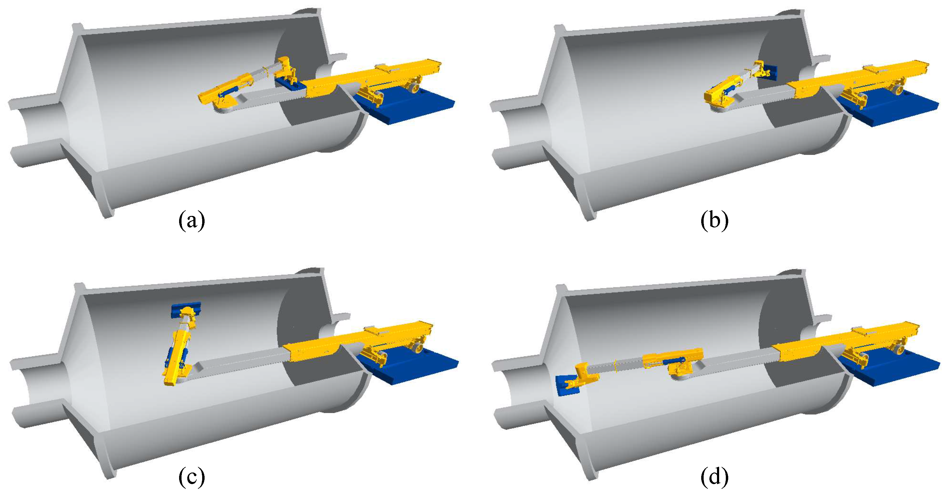
In actual grinding production, wear-resistant liners are installed inside the grinding mill and serve to protect the mill shell from the aggressive environment. Furthermore, the liners are distributed along the inner surface of the mill. The mill relining manipulator works inside the grinding mill. Figure 2 illustrates the liner installation process using a mill relining manipulator. First, as shown in Figure 2a, the liner is grabbed by the end effector from the transport trailer. This situation is the starting joint configuration of all other operations. Second, the manipulator needs to transfer the liner to the goal position to complete the exchange task. During motion, the liner is attached to the end effector, and they have the same orientation. Figure 2b–d present the desired goal joint configurations for liner installation in near conical, middle cylindrical, and far conical areas, respectively. At the goal position, end deformation must be taken into account to ensure end effector positioning accuracy.

3. Methodology

3.1. Overall Framework of Proposed Method

The purpose of the proposed method is to realize online calculation of the manipulator end effector deformation with a low FE simulation cost. Figure 3 is the overall framework of the proposed method, where two stages are designed in this paper: offline deformation dataset establishment and online calculation. First, to reduce the FE simulation cost, the manipulator is decomposed into two cantilever beams: the forearm and upper arm. Furthermore, the discrete joint values are selected based on the joint constraints to cover the entire joint space, and the details are presented in Table 4. It should be noted that, due to the left–right symmetry of the manipulator’s workspace, the discrete values of q 2 need to cover only the positive range. Consequently, permutations and combinations are conducted to obtain a total of 3528 sparse discrete joint configurations. This operation ensures that those configurations for FE analysis can cover the joint space as uniformly as possible. Second, for every joint configuration, a unique corresponding FE static model can be built. Furthermore, a force and moment transfer model is developed for the reverse force transmission from the forearm to the upper arm. The coupling relationship is in charge of the end effector displacement calculation caused by the upper arm deformation. Third, the offline deformation dataset can be achieved and used as a foundation for the following online end deformation calculation. In the online working stage, a trained neural network model is used as the online calculation algorithm to predict end effector deformation in real time.

3.2. Manipulator Decomposition and Force Analysis

To establish the offline dataset, all FE models with different joint configurations should be solved individually. To accelerate the FE analysis process, it is necessary to simplify and decompose the manipulator structure. The mill relining manipulator belongs to a special serial robotic arm, in which each link interacts with adjacent links through force and moment transmission. Therefore, the manipulator can be seen as a combination of multiple interconnected links. If this redundant manipulator is decomposed according to its degrees of freedom, seven links can be obtained after decomposition. Although this strategy is a complete abstraction of the manipulator’s structure, the inverse transmission of forces and moments is complex, and the problem of high FE simulation cost still exists. In this paper, as illustrated in Figure 4, the manipulator is further simplified by decomposing it into two independent cantilever beams, and FE simulations are subsequently conducted on each beam individually. Since the manipulator’s wrist exhibits a compact structure, small span, and high stiffness, we combine the wrist component with the forearm as a front cantilever beam. In addition, the upper arm can be seen as another individual cantilever beam. On this basis, only two spatial force systems need to be analyzed. It should be noted that the decomposition brings the problems of boundary distortion and loss of coupling effects. Therefore, to ensure the result’s accuracy during FE simulation, the reaction forces and moments generated by the forearm should be considered in solving the upper arm FE model.

3.3. Reaction Force and Moment Calculation

According to the force analysis shown in Figure 4, the upper arm cantilever beam is not only subjected to its own gravity, but also to the reaction forces and moments transmitted from the forearm at the turntable. In the local coordinate system O 1 , to support the end load and the forearm’s weight, the forearm cantilever beam generates a force F y 1 along the y-axis and moments M x 1 and M z 1 about the x-axis and z-axis, respectively, as indicated by the green arrow.
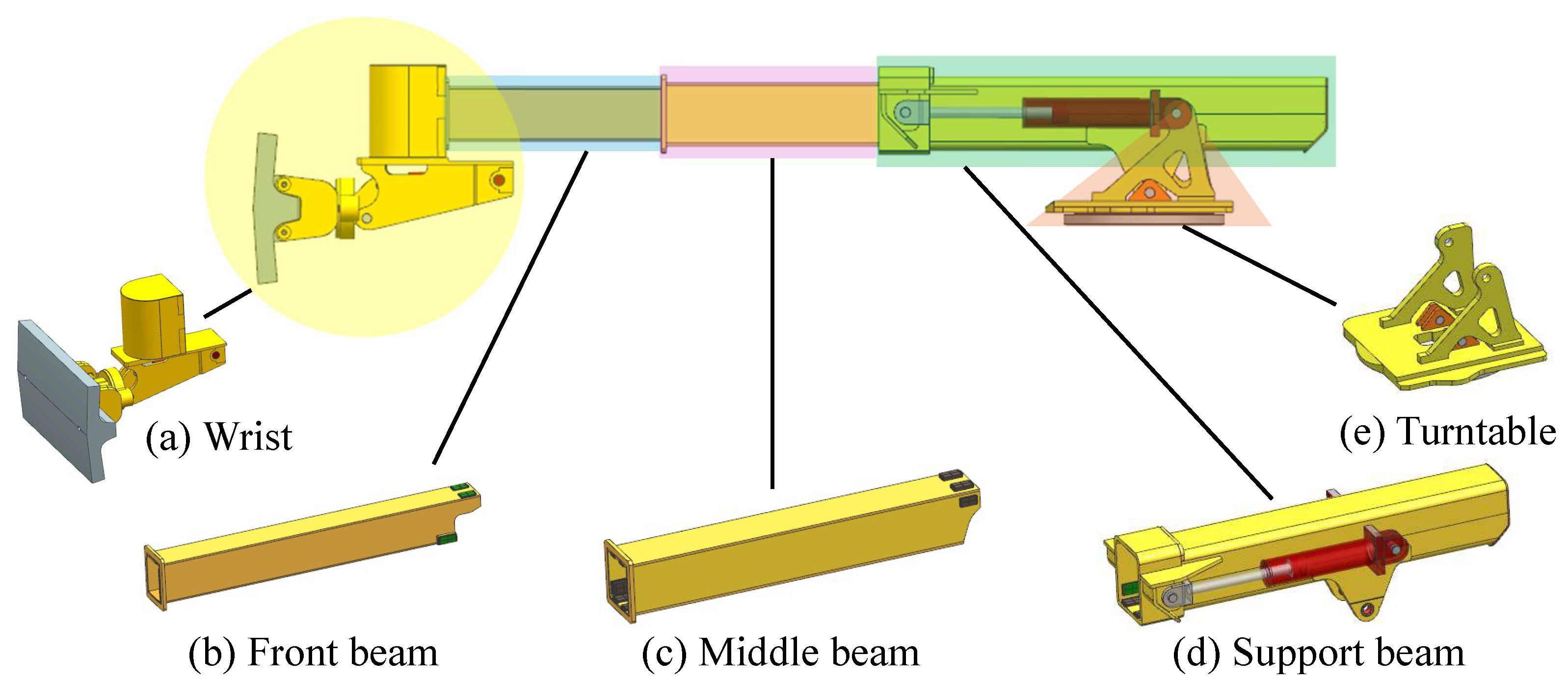
Therefore, the FE load conditions of the upper arm vary with the postures of the forearm; it is necessary to introduce an analytical method to calculate the reaction forces and moments. As shown in Figure 5, the forearm cantilever is further divided into five components: the wrist, front beam, middle beam, support beam, and the turntable. Since each component cannot be divided further, the center of mass coordinate is constant in its own local coordinate system. It should be noted that, due to the compact structure of the wrist, it is assumed that its three degrees of freedom remain unchanged during motion, and only the variations in joints q 2 , q 3 , and q 4 are considered. Consequently, the real-time reaction force and moment can be calculated through the forward kinematics model and the initial measured center of mass coordinates.
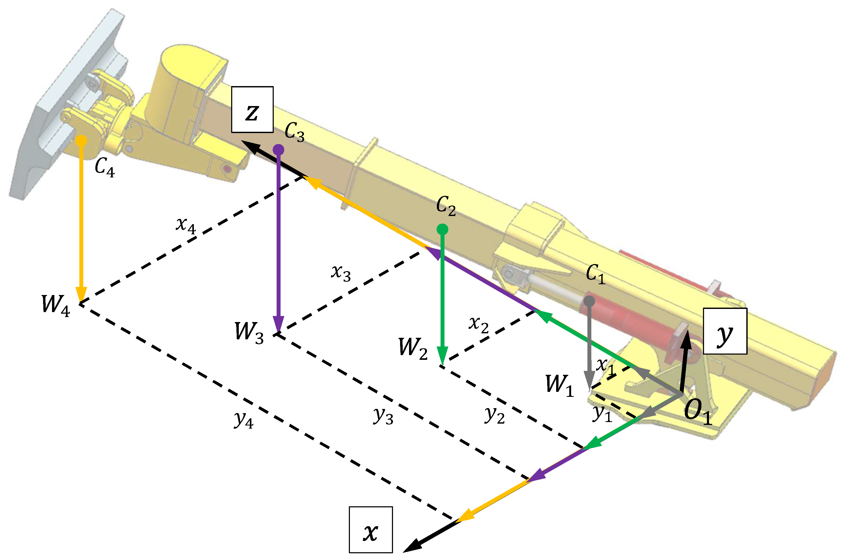
As illustrated in Figure 6, the weights of the forearm turntable, support beam, middle beam, front beam, and end mill liner are represented by W 0 , W 1 , W 2 , W 3 , W 4 , and their corresponding center of mass coordinates are denoted by C 0 , C 1 , C 2 , C 3 , C 4 . According to the theorem of resultant force and moment, the overall force generated by the forearm and end load on the O 1 coordinate system is equal to the cumulative gravitational forces of all associated components, as expressed in Equation (3). The moment M x is the sum of each component’s weight W i multiplied by its y i , as expressed in Equation (4). Since the center of the turntable nearly coincides with O 1 , the contribution of W 0 can be neglected in the moment calculation. The moment M z can be derived in the same way.
F y = i = 0 4 W i
M x = i = 1 4 w i y i
M z = i = 1 4 w i x i

3.4. Finite Element Static Models of Forearm and Upper Arm

The establishment of FE models is for solving the following simulation and obtaining end effector deformation in advance. In this paper, a 4.5-ton liner is used as the end load to establish the FE static models. The solid objects are used for FE analysis directly. The material of the manipulator’s structural parts is set as Q235 steel, with a yield strength of 235 MPa, an elastic modulus of 2.1 × 10 5 MPa, and a Poisson’s ratio of 0.3. The FE models of the forearm and upper arm are shown in Figure 7 and Figure 8, respectively. The boundary conditions of load constraints, fixed support, mesh elements, and mesh nodes are presented in Table 5. The forearm has both bonded and frictional connections, and the friction coefficient is 0.15. To improve computational efficiency, the unnecessary structural components of the mobile chassis are omitted to simplify the FE model. Furthermore, fixed supports and standard earth gravity are applied to the manipulator according to real working conditions.

3.5. Coupling Relationship Between Forearm and Upper Arm

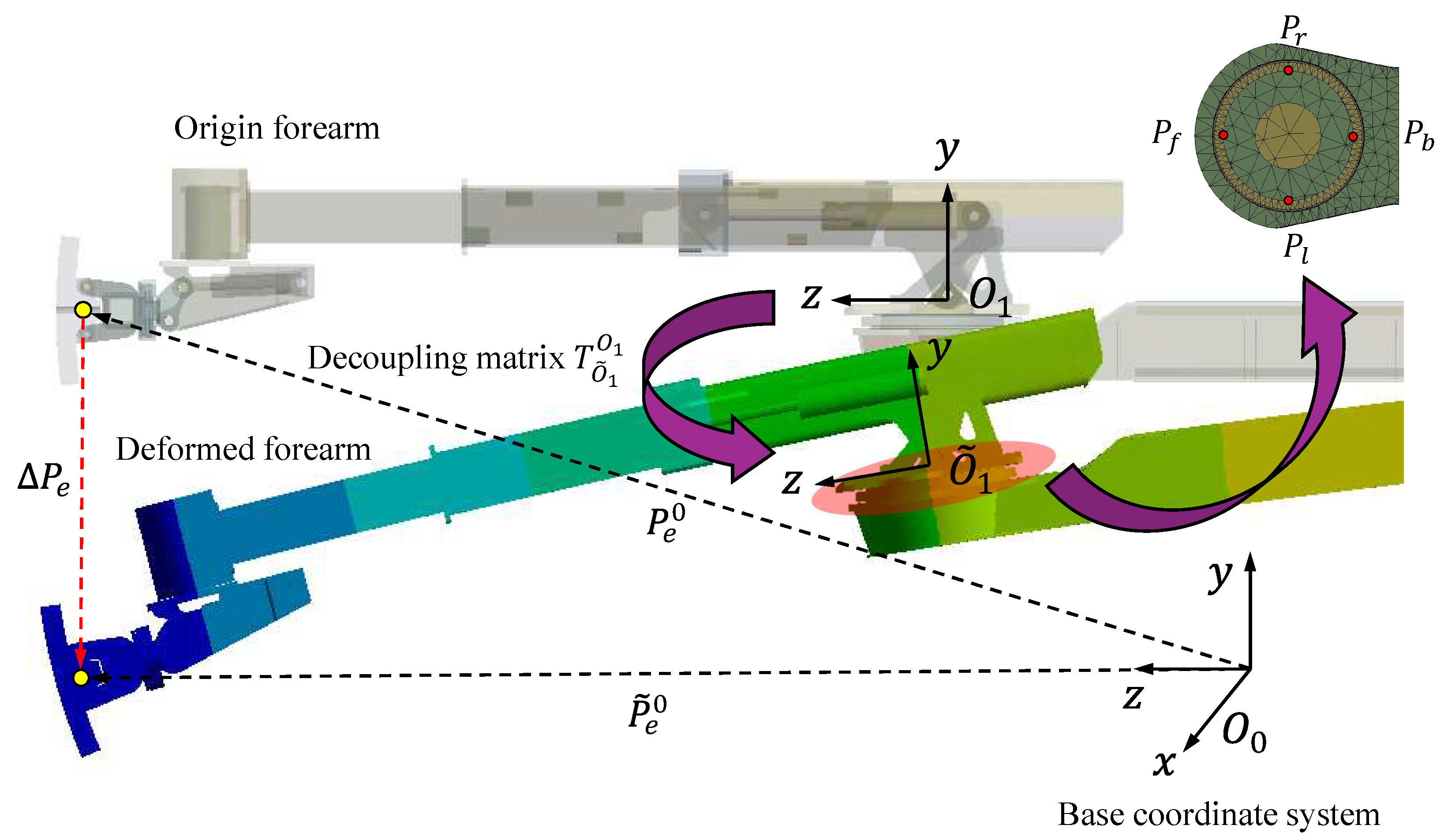
To avoid the lack of coupling caused by the manipulator decomposition, the coupling relationship should be analyzed and considered during the upper arm FE model solving. The forearm beam is assembled to the upper arm beam via the support turntable; the deformation of the upper arm inevitably affects the position of the end effector. The effect of upper arm deformation on the end effector position needs to be analyzed in detail, rather than a simplistic summation of the deformations at each beam end. In this section, a decoupling transformation matrix is proposed to calculate the end effector deformation caused by the upper arm deformation. Figure 9 shows the coupling relationship and decoupling principle of the upper arm deformation and end effector displacement. It can be seen that both the orientation and position of the local coordinate system O 1 have changed, and O 1 ˜ is the coordinate after deformation. As expressed in Equation (6), the decoupling transformation matrix T O 1 ˜ O 1 can be indirectly derived from the transformation matrix T O 1 ˜ O 0 , where T O 1 O 0 is a known invertible transformation matrix of O 1 relative to the base coordinate system O 0 . T O 1 ˜ O 0 can be derived by measuring the mesh nodes’ coordinate differences on the turntable of the upper arm after FE simulation. The measured points P r , P l , P f , and P b are designed to be evenly distributed around the turntable, as shown in Figure 9. As expressed in Equation (7), the normalized vector P r P l is used as the n component of the rotation matrix and P b P f for the a component. By utilizing the orthogonality of the rotation matrix, that is, o = a × n , the o component can be obtained. The position vector p of O 1 ˜ corresponds to the center of the circle defined by the four measured points. The end effector position difference vector Δ P e caused by this coupling relationship is calculated by Equation (8), where P e 0 and P e 0 ˜ represent the position vectors of the end effector in the O 0 coordinate system before and after deformation, respectively. P e 1 represents the theoretical position vector of the end effector, expressed in the coordinate system O 1 , without considering the forearm deformation. Finally, the y component of Δ P e is taken as the upper arm decoupled deformation u 2 .
T O 1 ˜ O 1 = ( T O 1 O 0 ) 1 · T O 1 ˜ O 0
T O 1 O 0 = n o a p 0 0 0 1
Δ P e = P e 0 ˜ P e 0 = T O 1 O 0 ( T O ˜ 1 O 1 I ) P e 1

3.6. Offline Deformation Dataset Establishment

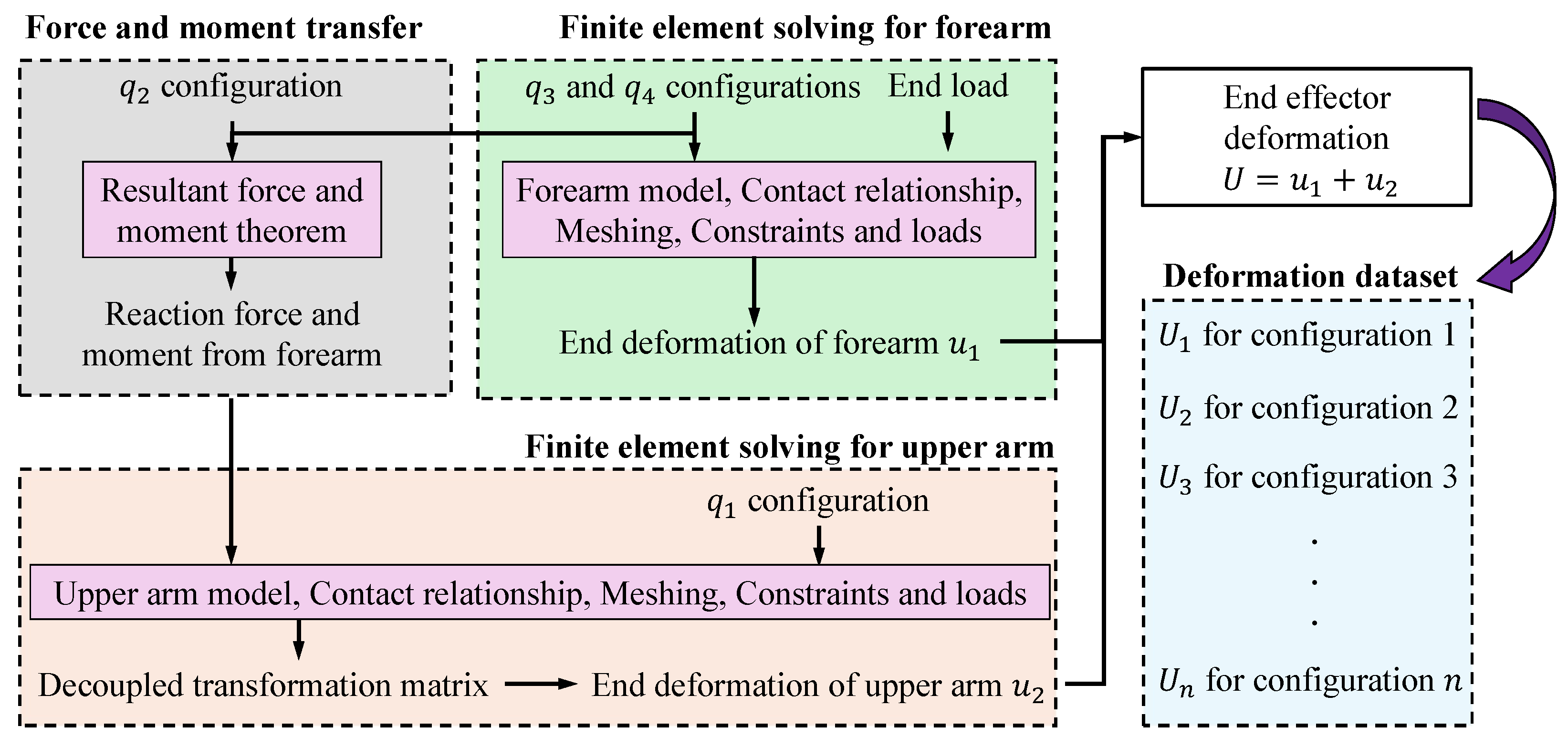
The offline deformation dataset is the foundation for the following online calculation. It is known that the changes in the manipulator’s posture result in varying deformations at the end effector. Therefore, all end effector deformations with different joint configurations need to be obtained through offline FE model solving. As shown in Figure 10, all preparations mentioned above are integrated in this section, including the force and moment transfer method, FE models for the forearm and upper arm, and the decoupling transformation matrix. In the forearm FE model, the end load and the configurations of joints q 3 and q 4 are inputs, and end deformation u 1 can be obtained after FE simulation solving. The left transfer model uses joints q 2 , q 3 , and q 4 as inputs to generate the reaction forces and moments, which are the input of the bottom FE model of the upper arm. Furthermore, the joint q 1 should also be considered during decoupling transformation to generate end deformation of the upper arm u 2 . Finally, the sum of u 1 and u 2 represents end effector deformation U in the current manipulator posture. Similarly, all FE models with different joint configurations are solved one after another, and the sparse discrete end deformation dataset { U 1 , U 2 , U 3 , …, U 3528 } can be achieved.

3.7. Kolmogorov-Arnold Network for Online End Deformation Calculation

Kolmogorov-Arnold representation theorem is an important conclusion in classical mechanics and dynamical systems theory [33]. In this theorem, a multivariate continuous function f : R n R m defined on a bounded domain can be represented as a finite superposition of single-variable functions through univariate functions and sums. There always exist continuous functions ϕ i : R R and ψ i , j [ 0 , 1 ] n R to obtain a smooth f : [ 0 , 1 ] n R through Equation (9).
y = f ( x 1 , x 2 , , x n ) = i = 1 2 n + 1 ϕ i j = 1 n ψ i , j ( x j )
Specifically, a complex nonlinear mapping between inputs and outputs can be represented through a finite number of continuous functions. Furthermore, Liu et al. [34] solved the problems of unlearnability in practice and proposed a new model training method, named the Kolmogorov-Arnold network (KAN). As for end effector deformation prediction tasks, the joints q 1 , q 2 , q 3 , , q k can be used to transfer into the network through the input layer. Different from Multilayer Perceptrons (MLPs), the activation functions ψ i , j in the hidden layer are learnable B-spline functions, which are smooth and flexible piecewise polynomials that enable high-precision approximation of complex functions while maintaining computational efficiency [35]. Consequently, the neuron g i can be obtained through a sum operation, as expressed in Equation (10). Next, the learnable activation functions ϕ i are involved in calculating g ˜ i through Equation (11). In the output layer, the predicted end deformation u ^ is achieved by summing all obtained neurons g ˜ i , as shown in Equation (12). To predict the end effector deformation of the mill relining manipulator, the architecture of the proposed KAN is shown in Figure 11.
g i = j = 1 k ψ i , j ( q j )
g ˜ i = ϕ i ( g i )
u ^ = i = 1 2 k + 1 g ˜ i

4. Visualization Analysis and Simulation Validation

4.1. End Effector Deformation Visualization

In a working space, end effector deformation visualization can help us to investigate the actual end effector position of different joint configurations. As shown in Figure 12, all the solved FE simulation solutions from the offline deformation dataset are plotted in the working space. To analyze the end deformation distribution, three projection maps are provided on the X–Y, Y–Z, and X–Z planes. Every end effector position is calculated by the forward kinematic model and expressed in the base coordinate system O 0 . A total of 3528 circles are displayed, and their colors represent the corresponding deformation magnitudes. It can be observed that the redder the color, the greater the deformation, while the bluer the color, the smaller the deformation. As illustrated in Figure 12c, deformation gradually increases along the positive direction of the Z-axis. In the 0 to 10,000 mm range, the main deformations fall between −15 mm and −90 mm, represented by blue circles, indicating that the deformations are relatively small. However, when the end effector moves into the range of 12,000 mm to 20,000 mm, the deformation increases significantly, ranging from −90 mm to −277.5 mm. The number of red circles accounts for a small proportion compared with the others and is primarily distributed at the distal end of the working space. The reason is that the upper arm and forearm are both significantly extended, resulting in the end effector being located at a far distance from the fixed base support. As a result, the moment increases, leading to greater bending deformation. Therefore, for the liners installed at the far conical surface, more compensation and adjustment should be given.

4.2. Manipulator Decomposition Necessity

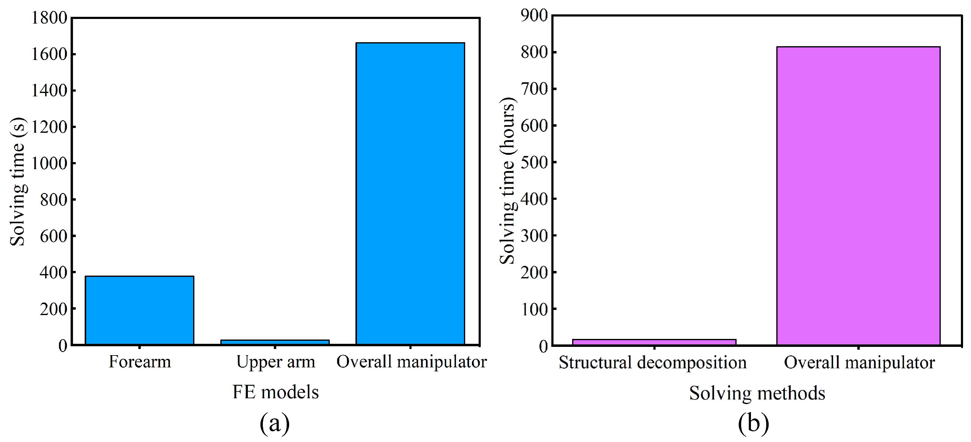
In this section, the necessity of the proposed separate FE modeling and decoupling operation is discussed. One of the key advantages of manipulator decomposition is the significant improvement in computational efficiency. The average FE solving times are presented in Table 6. For the separate FE models, the forearm and upper arm individual solving needs t 1 = 377 s and t 2 = 26 s to obtain the end deformation results. However, the solving time of the overall manipulator FE model reaches t 3 = 1663 s, which is approximately 4.1 times longer than the total time of the individual components, as presented in Figure 13a. In addition, the total solving time of different methods should be calculated to further demonstrate the advantages of separate solving. As shown in Table 4, joints q 2 and q 3 each have six different configurations, while joints q 1 and q 4 each have seven configurations. A total of 1764 FE models are established and should be solved. Therefore, the establishment of the end deformation dataset needs about 814.87 h (33.95 days), which is inefficient and unacceptable. In comparison, the proposed separate modeling method completes all FE sample solving only needs 17.14 h, according to the formula t 1 × ( 6 × 7 ) + t 2 × ( 6 × 7 × 6 × 7 ) . As presented in Figure 13b, manipulator decomposition has a huge advantage. On the other hand, the individual solving for the upper arm can be conducted through scripting automation in ANSYS 2022 R1 since the reaction force and moment are calculated as discussed in Section 3.3. Conversely, overall FE modeling requires manual configuration adjustments, which makes it infeasible and inefficient for establishing the end deformation dataset. The advantages and weaknesses of each solving method are summarized in Table 7, which explains the reason why structural decomposition and separate solving are necessary.

4.3. Effectiveness Validation of Manipulator Decomposition

The experiments are designed in three parts: effectiveness validation, error cause analysis, and superiority demonstration. First, the comparison experiments between the overall FE and the separate FE are carried out to verify the effectiveness of the proposed manipulator decomposition. Second, the potential errors caused by the separate FE modeling are analyzed. Third, an actual liner exchange case is involved to further demonstrate the superiority of the proposed online prediction method. To facilitate reproducibility, the experimental setup is described as follows. The following experiments have the same end load: a 4.5-ton liner mounted on the end effector. Furthermore, as discussed in Section 3.4, all FE static models have the same setting, including mesh size, material properties, and gravity constraint. The measurement point for end deformation is located at the liner gripping pin on the end effector. In ANSYS, this value can be obtained through the probe function. However, in a real hardware experiment, the sensor should be installed in the same position, and a laser tracker system is required to measure the posture of the end effector. In addition, all the following simulations and algorithms are tested on a personal computer equipped with an AMD Ryzen 5600 processor and 32 GB of RAM.

4.3.1. Validation in Fully Extended Configuration

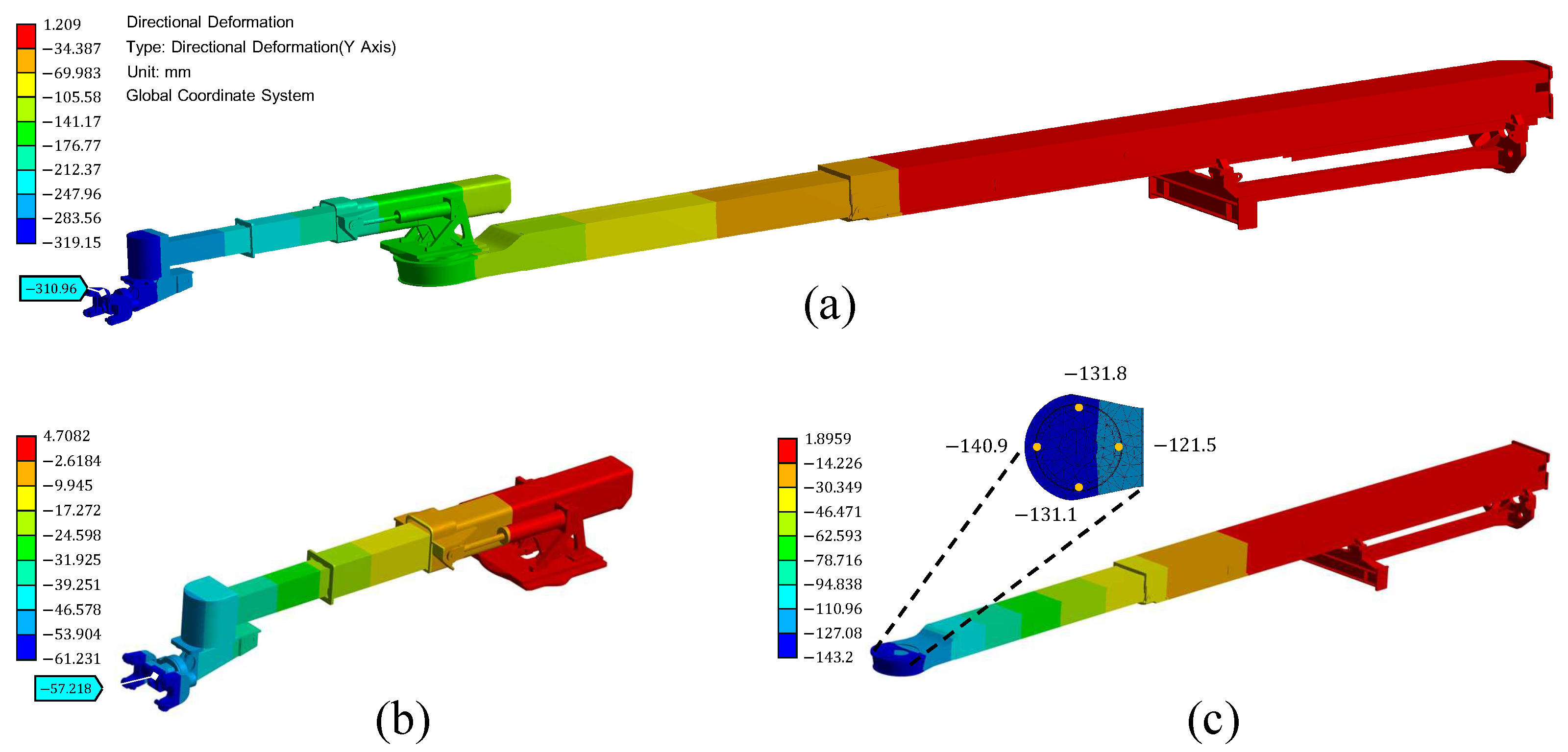
To verify the effectiveness of the proposed manipulator decomposition method, two common manipulator postures are selected to solve and compare with the overall FE simulations. As shown in Figure 14, the first posture is the fully extended configuration, where the center of mass is farthest from the fixed support and is in the worst working condition. In this posture, end effector deformation is greatest because the manipulator has to withstand the maximum moment. The overall FE simulation result is shown in Figure 14a, and the end effector deformation is −310.9 mm. As shown in Figure 14b, the separate FE simulation result of the forearm beam is −57.2 mm. For end deformation caused by upper arm deformation, the result cannot be obtained directly through the FE simulation solution. It is necessary to establish the decoupling transformation matrix T O 1 O 1 first according to the designed measured points. As shown in Figure 14c, based on the deformation differences in P r , P l , P f , and P b , the decoupled deformation u 2 = −250.6 mm can be obtained. Detailed results are shown in Table 8, where the end effector deformation of the separate FE solving is −307.8 mm, showing a difference of 3.1 mm compared with the overall FE simulation result.

4.3.2. Validation in 90° Rotation Configuration

As shown in Figure 15, the rotation configuration is obtained by rotating the forearm 90° from the fully extended configuration. This posture is commonly used for installing the sidewall liners of the grinding mill. Similarly, the deformation results can be obtained and are shown in Table 9. The overall FE solution is −230.2 mm, which is smaller than the fully extended configuration due to the reduction in the action moment. The separate FE solutions for the upper arm and forearm are u 1 = −57.2 mm and u 2 = −167.4 mm, respectively. The deformation discrepancy between the separate FE analysis and overall FE simulation is 5.6 mm, which is within the allowable error range for this heavy-duty manipulator.

4.4. Simulation Error Analysis

From the above comparison experiments, it can be found that the results of the overall and separate FE simulations have small errors in end deformation. The reason is that individual separate FE solving has two main problems: coupling relationship ignorance and boundary condition distortion. Fortunately, the coupling relationship is considered and discussed in Section 3.5, and the proposed decoupling matrix can solve the effect of upper arm deformation on end effector positioning accuracy. However, for the separate forearm FE model, the actual fixed support condition at the turntable cannot be known in advance. For the same joint configuration, the boundary conditions of separate and overall FE simulations are shown in Figure 16a and b, respectively. In the overall FE simulation, there is a twist angle β at the plane of the turntable, which is different from the theoretical fixed support in the separate FE simulation. Furthermore, this twist angle can only be obtained from the overall FE solution. Although this error cannot be considered in our proposed method, the effects are limited and acceptable, as elaborated in the following discussion.
A quantitative analysis is conducted to investigate the effect of forearm boundary distortion. As presented in Table 10, the FE models with seven different configurations of the joint q 4 are solved to find out the error changes across the entire workspace. Based on the range of twist angles generated by the overall FE simulation, 11 different fixed support conditions (twist angle β ) are designed to assess the negative influence of boundary condition distortion. It can be observed that end effector deformation decreases as the twist angle increases, which can be explained by the reduction in the reaction moment. In the fully extended configuration, the difference between the minimum and maximum values is only 2.9 mm. Although the boundary distortion errors arising from the structural decomposition are inevitable, the influence is limited and insignificant for the mill relining manipulator.

4.5. Effectiveness Validation of Online End Deformation Calculation

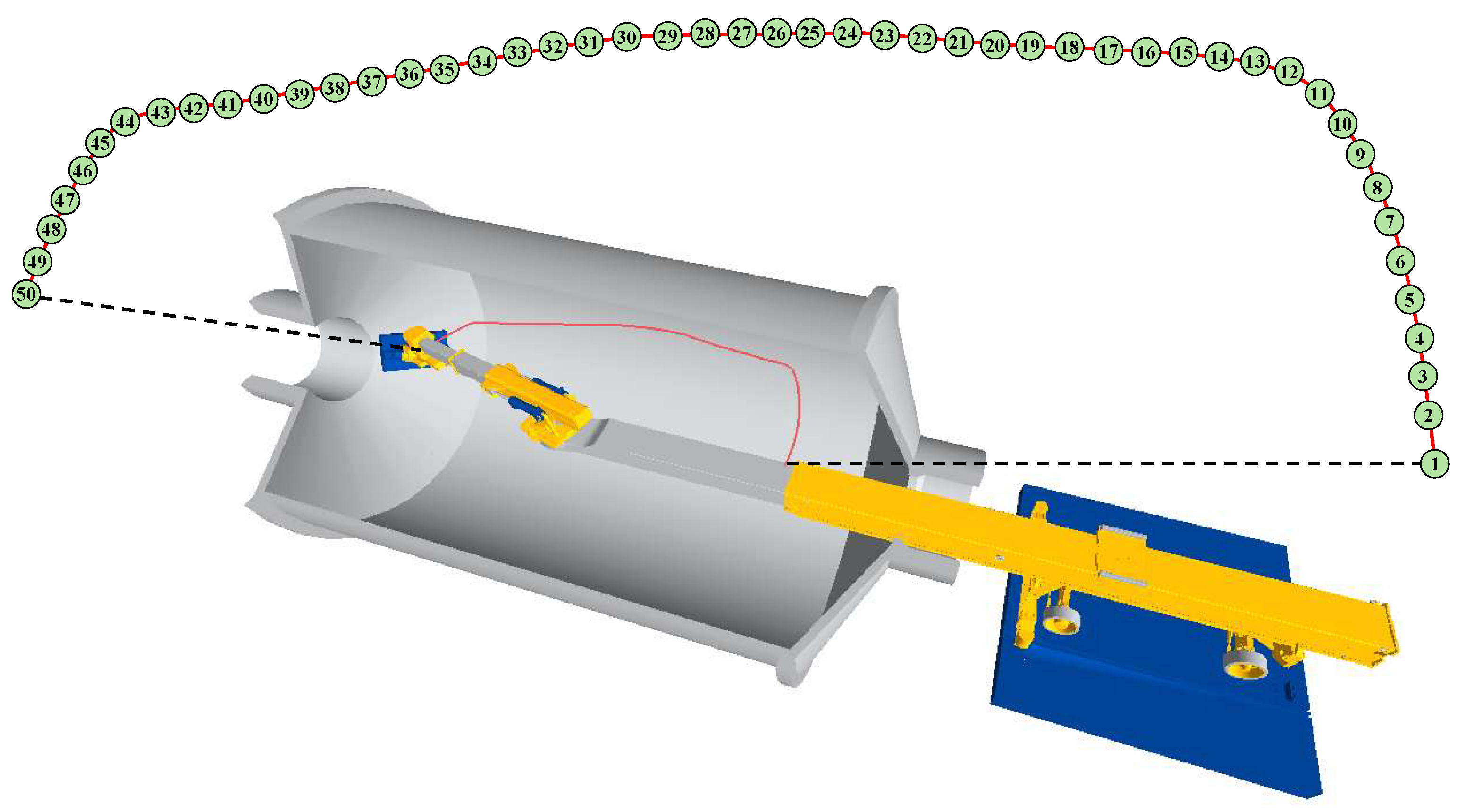
For the above-mentioned two special joint configurations, the end deformation can be directly found from the established offline discrete deformation dataset. However, the end effector deformation of random joint configurations requires the proposed online calculation algorithm. Therefore, this section focuses on validating the significance of the decoupling operation and the effectiveness of the proposed KAN online prediction algorithm. As presented in Figure 17, the mill liner has to be moved from the transfer cart to the target far conical surface. The red trajectory illustrates the motion path of the manipulator’s end effector. For this liner exchange task, all joint configurations are random and not included in the offline dataset, indicating that this simulation experiment is closer to the practical engineering application. It should be noted that this task assumes the manipulator is operated at a low speed. Therefore, gravity is the dominant factor on end deformation during this dynamic process rather than the inertial, Coriolis, and centrifugal forces. On this basis, the end deformation for each joint configuration can be calculated using FE static models.
Each path node is associated with a corresponding joint configuration. Therefore, from the entire motion path, 50 path nodes are selected and used as the test samples to predict end effector deformation. It can be seen that the selected path nodes are uniformly distributed along the end trajectory. Furthermore, four other solving algorithms are introduced as the comparison groups to demonstrate the superiority of the proposed method. As shown in Table 11, IJDW denotes the interpolation algorithm based on joint distance weight, while the coupling relationship is not considered. Different from IJDW, IJDW-D takes the decoupling operation into account so that the significance of the proposed decoupling method can be verified through these comparison experiments. The Radial Basis Function (RBF) [36] and MLP are involved to demonstrate the advantage of the proposed KAN method in the field of neural networks. KAN-4 and KAN-7 are the proposed online end deformation prediction algorithms based on the KAN neural network. For KAN-4, the designed inputs are q 1 , q 2 , q 3 , and q 4 , which are consistent with the dimensions of the established offline dataset. However, KAN-7 denotes that the architecture of KAN has seven input neurons, that is, q 1 to q 7 . It should be noted that the values of q 5 to q 7 are 0 during training, whereas the actual configurations are used during end deformation prediction. All joint values are normalized before being input into the network. All prediction algorithms have one output representing end deformation. Except for the RBF, the other networks have 10 hidden neurons for model fitting. Due to the designed network having few parameters, Levenberg–Marquardt (LM) [37] is employed as the optimization strategy instead of Adaptive Moment Estimation (Adam) [38] or Stochastic Gradient Descent (SGD) [39]. LM is a Jacobian-based training algorithm and has a high convergence speed. The model is considered to have converged when the gradient norm falls below 1 × 10 6 or the maximum iteration number of 200 is reached. Different from learnable activation functions in the KAN, the activation functions of the MLP network in the hidden and output layers are set as tansig and purelin, respectively. Unlike MLP, the KAN has another parameter of the order of the B-spline curve, which is set as 3 in this study. To avoid overfitting and underfitting, the spread of RBF is set as 10 based on the grid search method. Although the density of the established end deformation dataset is sparse and uniformly distributed, L1-norm and L2-norm regularization methods are also involved during KAN training, each with a coefficient of 1 × 10 5 .
In the following experiments, five metrics are used in this paper to evaluate the performance of different methods: coefficient of multiple determination ( R 2 ), mean absolute error (MAE), mean absolute percentage error (MAPE), root mean square error (RMSE), and mean square error (MSE). Their calculation formulas are expressed in Equations (13)–(17), where u i is the reference value generated by the overall manipulator FE solving, u ^ i denotes the predicted result by different algorithms, and u ¯ i represents the mean value of all u i .
R 2 = 1 i = 1 n ( u i u ^ i ) 2 i = 1 n ( u i u ¯ ) 2
MAE = 1 n i = 1 n u i u ^ i
MAPE = 100 % n i = 1 n u ^ i u i u i
MSE = 1 n i = 1 n ( u i u ^ i ) 2
RMSE = 1 n i = 1 n ( u i u ^ i ) 2
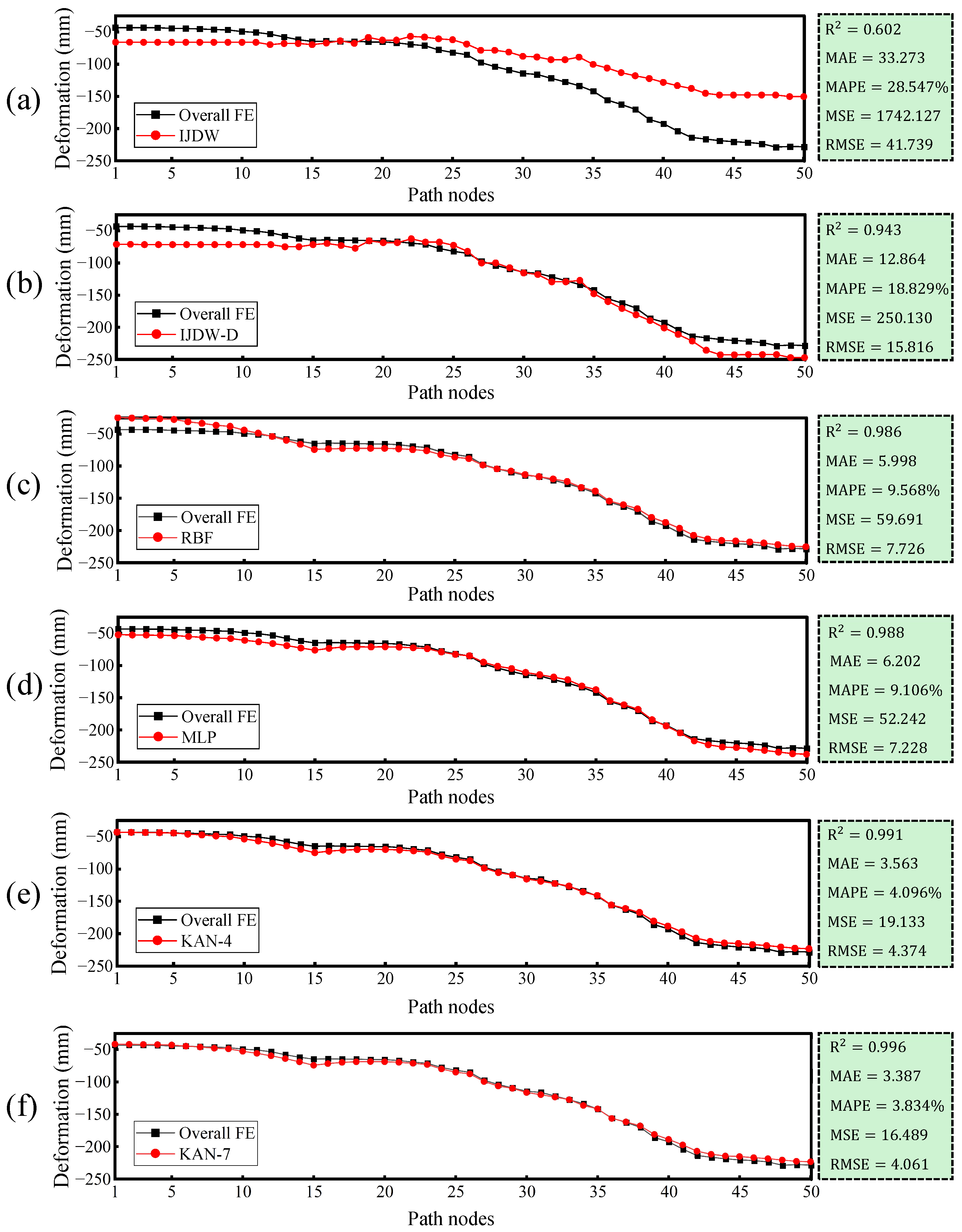
As presented in Table 12, all joint configurations of the 50 path nodes are used as test samples. In the simulation experiment, the overall manipulator FE model is solved, and its results are used as the reference. Based on the established offline end deformation dataset, the different algorithms are used to solve each FE model of each path node. As presented in Table 13, the predicted end effector deformation by IJDW is distorted due to the lack of consideration of the coupling relationship. Especially for the remote path nodes, the maximum end deformation error reaches 77.9 mm. As presented in Figure 18a, an X-shaped comparison result is observed between the reference and predicted values. The explanation is that, as the extension length increases, the coupling effect between the forearm and the upper arm becomes more pronounced. Compared with IJDW, the end deformation errors of IJDW-D are reduced due to the incorporation of the decoupling operation. As illustrated in Figure 18b, all metrics have a great improvement. For instance, R 2 has been increased to 0.943 from 0.602. Although the effectiveness and necessity of the proposed decoupling method are demonstrated through this comparison experiment, the end deformation prediction accuracy remains insufficient. Therefore, the neural network is introduced to further improve the performance of end deformation prediction. It can be found that RBF and MLP neural networks with a decoupling operation further reduce the prediction errors, particularly at both boundary nodes. As shown in Figure 18c,d, the trends of the red and black curves tend to coincide, and the corresponding R 2 values indicate that the models exhibit high fitting performances. The best performance is achieved by the proposed KAN-based network since it is more suitable for this lightweight fitting problem. As shown in Figure 18f, KAN-7 exhibits a slight improvement over KAN-4. The reason is that the additional three inputs enrich the learnable features during model training. For the results achieved from KAN-7, the values of R 2 , MAE, MAPE, MSE, and RMSE are 0.996, 3.387, 3.834%, 16.489, and 4.061, respectively. Compared with the MLP algorithm, the MAE, MAPE, MSE, and RMSE decrease by 2.815, 5.719%, 35.753, and 3.167, respectively, while the R 2 value increases by 0.008. The capability of end effector deformation prediction is further improved. The superiority of the KAN model is further evidenced by the red curve in Figure 18f, which almost coincides with the black reference line. Compared with other algorithms, the KAN has smaller parameters, and its learnable activation functions have a better capability for fitting nonlinear mapping. In addition, the spline-based activation functions of the KAN can focus not only on global features but also on local features. For instance, changes in end deformation arise from modifications to an individual joint. All the above discussion explains why KAN can achieve excellent performance across all metrics. Although the end trajectory comparison between the overall FE simulation and the predicted deformation is not visually significant at the scale of the whole grinding mill, we also provide simulation videos in the Supplementary Materials.
In addition, it should be clarified that the average prediction time for one sample is 0.016 s. This fast calculation method can be deployed on devices with limited computational capability, such as control systems based on programmable logic controllers (PLCs) or embedded platforms. In contrast, the overall FE static method is more suitable for the laboratory environment equipped with high-performance computers rather than real industrial scenarios. The reason is that its long model-solving time makes it unable to provide real-time feedback to a manipulator’s control system. In addition, if different payloads are incorporated as variables to expand the training dataset, the model will exhibit higher generalizability in predicting end deformation under varying liner weights. In summary, the proposed online end deformation calculation method can satisfy real-time manipulator motion control and can be integrated into a digital twin system.

5. Conclusions

In this study, we aimed to reduce FE simulation costs and improve the end effector positioning accuracy of a mill relining manipulator. This paper proposed an online calculation method to predict end effector deformation caused by heavy end loads and self-gravity effects. Based on the manipulator decomposition, reaction force and moment transfer, coupling relationship analysis, FE static model solving, offline deformation dataset establishment, and KAN, this paper offers a feasible framework for real-time calculation of end deformation for mill liner exchange tasks. The main conclusions are outlined as follows:
(1)
To save FE model solving time, the mill relining manipulator is decomposed into two independent cantilever beams: the forearm and the upper arm. On this basis, the reaction force and moment are analyzed for reverse force transmission, and the decoupling transformation matrix is proposed to prevent the lack of a coupling relationship caused by manipulator decomposition.
(2)
According to the selected discrete joint configurations, 3528 FE static models are built and solved to establish the offline end deformation dataset. Based on this dataset, joints q 1 , q 2 , q 3 , and q 4 can be used to calculate the current end effector deformation.
(3)
By introducing the KAN, an online prediction model can be trained to obtain real-time end effector deformation.
(4)
Through visualization analysis, the end deformation distribution is exhibited in the working space. Furthermore, the feasibility and effectiveness of the manipulator decomposition and online calculation algorithms are demonstrated through several comparison experiments. For a mill liner exchange task, the predicted error and calculation speed can satisfy the requirements of real-time motion control.
In addition, there are also some limitations in this study. Physical validation on a real mill relining manipulator can further demonstrate the effectiveness of the proposed method. However, the prototype platform is still under development, and the performance of the proposed method on hardware equipment cannot be demonstrated at this time. As the proposed method is based on FE static analysis, it is not applicable to prediction tasks during manipulator motion at high speeds. In such scenarios, end effector deformation is not only affected by gravity but also by inertia, Coriolis, and centrifugal effects. Therefore, some important works should be conducted in the future. First, further validation will be carried out with the prototype platform using a laser tracker system. Second, a dynamic model will be established to study end deformation during motion with different speeds. Third, a digital twin system will be established to integrate the proposed online calculation method with other control or diagnostic modules. On this basis, a smart manufacturing system can be developed for the maintenance of the entire grinding mill equipment. In addition, some potential directions for future investigation are discussed here. To address the limited size of the established end deformation discrete dataset, generative adversarial networks (GANs) can be introduced for data augmentation. Transfer learning can also be employed to reduce the model training cost for new, heavy-duty end deformation prediction. The proposed method is implemented within an open-loop control system. Therefore, another extended direction is to develop a closed-loop system to further enhance task performance. For instance, visual recognition can be introduced for end positioning, while the end deformation prediction model proposed in this paper can be used as a preprocessing module to reduce online adjustment time.

Supplementary Materials

The following supporting information can be downloaded at: https://www.mdpi.com/article/10.3390/machines14010021/s1.

Author Contributions

Conceptualization, M.W. and Y.X.; methodology, M.W.; software, M.W.; validation, Y.X.; formal analysis, M.W.; investigation, M.W. and S.L.; resources, Y.X. and Y.B.; data curation, M.W. and Y.B.; writing—original draft preparation, M.W.; writing—review and editing, M.W., Y.X. and J.L.; visualization, M.W. and S.L.; supervision, Y.X. and J.L.; project administration, Y.X. All authors have read and agreed to the published version of the manuscript.

Funding

This research is supported by the Key Research and Development Special Project of Henan Province, China, grant number 231111221500.

Data Availability Statement

The data that support the findings of this study are available from the corresponding author upon reasonable request.

Conflicts of Interest

Authors Yujun Xue and Yunhua Bai were employed by the company CITIC Heavy Industries Co., Ltd.; Author Yunhua Bai were employed by the company Luoyang CITIC HIC Automation Engineering Co., Ltd. The remaining authors declare that the research was conducted in the absence of any commercial or financial relationships that could be construed as a potential conflict of interest.

References

  1. Jiao, J.; Tian, W.; Zhang, L.; Li, B.; Hu, J.; Li, Y.; Li, D.; Zhang, J. Variable Stiffness Identification and Configuration Optimization of Industrial Robots for Machining Tasks. Chin. J. Mech. Eng. 2022, 35, 291–306. [Google Scholar] [CrossRef]
  2. Ma, S.; Deng, K.; Lu, Y.; Xu, X. Robot error compensation based on incremental extreme learning machines and an improved sparrow search algorithm. Int. J. Adv. Manuf. Technol. 2023, 125, 5431–5443. [Google Scholar] [CrossRef]
  3. Cai, J.; Lei, T. An autonomous positioning method of tube-to-tubesheet welding robot based on coordinate transformation and template matching. IEEE Robot. Autom. Lett. 2021, 6, 787–794. [Google Scholar] [CrossRef]
  4. He, Y.; Xia, Y.; Xu, Z.; Yao, J.; Ning, B.; Xiao, X. A 6-m Tunnel Boring Machine Steel Arch Splicing Manipulator. Chin. J. Mech. Eng. 2022, 35, 134–147. [Google Scholar] [CrossRef]
  5. Gu, J.; He, S.; Dai, J.; Wei, D.; Yan, H.; Tan, C.; Wang, Z.; Si, L. A Walking Trajectory Tracking Control Based on Uncertainties Estimation for a Drilling Robot for Rockburst Prevention. Machines 2024, 12, 298. [Google Scholar] [CrossRef]
  6. Zhang, X.; Huang, M.; Lei, M.; Tian, H.; Chen, X.; Tian, C. Improved Rapid-Expanding-Random-Tree-Based Trajectory Planning on Drill ARM of Anchor Drilling Robots. Machines 2023, 11, 858. [Google Scholar] [CrossRef]
  7. Zhang, J.; Wang, Y.; Che, L.; Wang, N.; Bai, Y.; Wang, C. Workspace analysis and motion control strategy of robotic mine anchor drilling truck manipulator based on the WOA-FOPID algorithm. Front. Earth Sci. 2022, 10, 954547. [Google Scholar] [CrossRef]
  8. Liu, W.; Zou, X.; Wen, Z.; Cheng, J.; Zuo, Y.; Zhang, C.; Liu, H.; Tao, F. Digital Twin-Based Production-Logistics Synchronization System for Satellite Mass Assembly Shop-Floor. Chin. J. Mech. Eng. 2024, 37, 43–67. [Google Scholar] [CrossRef]
  9. Liu, Y.; Yi, W.; Feng, Z.; Yao, J.; Zhao, Y. Design and motion planning of a 7-DOF assembly robot with heavy load in spacecraft module. Robot. Comput.-Integr. Manuf. 2024, 86, 102645. [Google Scholar] [CrossRef]
  10. Korendiy, V.; Kachur, O.; Pylyp, M.; Karpyn, R.; Augousti, A.; Lanets, O. Design and kinematic analysis of a robotic manipulator for controlling fire monitors. Ukr. J. Mech. Eng. Mater. Sci. 2025, 11, 10–26. [Google Scholar] [CrossRef]
  11. Wang, Q.; Wu, H.; Song, Y.; Handroos, H.; Cheng, Y.; Qin, G. Parameter identification of heavy-duty manipulator using stochastic gradient Hamilton Monte Carlo method. IEEE Access 2023, 11, 78561–78583. [Google Scholar] [CrossRef]
  12. Yahyaei, M.; Powell, M.; Toor, P.; Tuxford, A.; Limpus, A. Relining efficiency and liner design for improved plant performance. Miner. Eng. 2015, 83, 64–77. [Google Scholar] [CrossRef]
  13. Pural, Y.E.; Ledezma, T.; Hilden, M.; Forbes, G.; Boylu, F.; Yahyaei, M. Application of Machine Learning for Generic Mill Liner Wear Prediction in Semi-Autogenous Grinding (SAG) Mills. Minerals 2024, 14, 1200. [Google Scholar] [CrossRef]
  14. Liu, Y.; Shi, W.; Chen, P.; Cheng, L.; Ding, Q.; Deng, Z. Variable Curvature Modeling Method of Soft Continuum Robots with Constraints. Chin. J. Mech. Eng. 2023, 36, 63–73. [Google Scholar] [CrossRef]
  15. Naclerio, N.D.; Karsai, A.; Murray-Cooper, M.; Ozkan-Aydin, Y.; Aydin, E.; Goldman, D.I.; Hawkes, E.W. Controlling subterranean forces enables a fast, steerable, burrowing soft robot. Sci. Robot. 2021, 6, eabe2922. [Google Scholar] [CrossRef]
  16. Yang, Y.; Niu, T.; Zheng, Y.; Zhao, Y.; Qi, Y.; Zhong, S. End Positioning Accuracy Improvement for Soft Arms Under Various Loads. IEEE Sensors J. 2023, 24, 5237–5245. [Google Scholar] [CrossRef]
  17. He, Z.; Lian, B.; Li, Q.; Zhang, Y.; Song, Y.; Yang, Y.; Sun, T. An error identification and compensation method of a 6-DoF parallel kinematic machine. IEEE Access 2020, 8, 119038–119047. [Google Scholar] [CrossRef]
  18. He, L.; Li, Q.; Zhu, X.; Wu, C. Kinematic calibration of a three degrees-of-freedom parallel manipulator with a laser tracker. J. Dyn. Syst. Meas. Control 2019, 141, 031009. [Google Scholar] [CrossRef]
  19. Xiang, W.; Chen, J.; Li, H.; Chai, Z.; Lou, Y. Research on End-Effector Position Error Compensation of Industrial Robotic Arm Based on ECOA-BP. Sensors 2025, 25, 378. [Google Scholar] [CrossRef] [PubMed]
  20. Li, R.; Ding, N.; Zhao, Y.; Liu, H. Real-time trajectory position error compensation technology of industrial robot. Measurement 2023, 208, 112418. [Google Scholar] [CrossRef]
  21. Li, B.; Tian, W.; Zhang, C.; Hua, F.; Cui, G.; Li, Y. Positioning error compensation of an industrial robot using neural networks and experimental study. Chin. J. Aeronaut. 2022, 35, 346–360. [Google Scholar] [CrossRef]
  22. Min, K.; Ni, F.; Chen, Z.; Liu, H.; Lee, C.H. A robot positional error compensation method based on improved kriging interpolation and Kronecker products. IEEE Trans. Ind. Electron. 2023, 71, 3884–3893. [Google Scholar] [CrossRef]
  23. Luo, G.; Zou, L.; Wang, Z.; Lv, C.; Ou, J.; Huang, Y. A novel kinematic parameters calibration method for industrial robot based on Levenberg-Marquardt and Differential Evolution hybrid algorithm. Robot. Comput.-Integr. Manuf. 2021, 71, 102165. [Google Scholar] [CrossRef]
  24. Yang, M.; Shen, J.; Gao, P.; Zhang, X.; Wang, J. Design of Continuum Robot and its Compensation Strategy for Loss of GuidePath. China Mech. Eng. 2025, 1–11. Available online: https://link.cnki.net/urlid/42.1294.th.20250328.1605.006 (accessed on 31 March 2025). (In Chinese).
  25. Hu, J.; Liu, T.; Zeng, H.; Chua, M.X.; Katupitiya, J.; Wu, L. Static modeling of a class of stiffness-adjustable snake-like robots with gravity compensation. Robotics 2022, 12, 2. [Google Scholar] [CrossRef]
  26. Wang, W.; Tian, W.; Liao, W.; Li, B.; Hu, J. Error compensation of industrial robot based on deep belief network and error similarity. Robot. Comput.-Integr. Manuf. 2022, 73, 102220. [Google Scholar] [CrossRef]
  27. Chen, G.; Sun, F.; Li, T.; Shao, W. Accuracy Compensation for a Lunar Sampling Manipulator with ElasticDeformation. J. Nanjing Univ. Aeronaut. Astronaut. Sci. Ed. 2021, 53, 1–10. [Google Scholar] [CrossRef]
  28. Montalvo, W.; Escobar-Naranjo, J.; Garcia, C.A.; Garcia, M.V. Low-cost automation for gravity compensation of robotic arm. Appl. Sci. 2020, 10, 3823. [Google Scholar] [CrossRef]
  29. Zhong, J.; Jiang, W.; Zhang, Q.; Zhang, W. Design and Simulation of a Seven-Degree-of-Freedom Hydraulic Robot Arm. Actuators 2023, 12, 362. [Google Scholar] [CrossRef]
  30. Zhang, D.; Wei, B. Study on Payload Effects on the Joint Motion Accuracy of Serial Mechanical Mechanisms. Machines 2016, 4, 21. [Google Scholar] [CrossRef]
  31. Wang, M.; Xue, Y.; Li, J.; Li, S.; Bai, Y. Digital Twin System for Mill Relining Manipulator Path Planning Simulation. Machines 2025, 13, 823. [Google Scholar] [CrossRef]
  32. Sung, M.; Choi, Y. Algorithmic Modified Denavit–Hartenberg Modeling for Robotic Manipulators Using Line Geometry. Appl. Sci. 2025, 15, 4999. [Google Scholar] [CrossRef]
  33. Braun, J.; Griebel, M. On a constructive proof of Kolmogorov’s superposition theorem. Constr. Approx. 2009, 30, 653–675. [Google Scholar] [CrossRef]
  34. Liu, Z.; Wang, Y.; Vaidya, S.; Ruehle, F.; Halverson, J.; Soljačić, M.; Hou, T.Y.; Tegmark, M. Kan: Kolmogorov-arnold networks. arXiv 2024, arXiv:2404.19756. [Google Scholar]
  35. Igelnik, B.; Parikh, N. Kolmogorov’s spline network. IEEE Trans. Neural Netw. 2003, 14, 725–733. [Google Scholar] [CrossRef] [PubMed]
  36. Shen, L.; Mao, P.; Fang, Q.; Wang, J. A Trajectory Tracking Approach for Aerial Manipulators Using Nonsingular Global Fast Terminal Sliding Mode and an RBF Neural Network. Machines 2022, 10, 1021. [Google Scholar] [CrossRef]
  37. Moré, J.J. The Levenberg-Marquardt algorithm: Implementation and theory. In Proceedings of the Numerical Analysis: Proceedings of the Biennial Conference, Dundee, UK, 28 June–1 July 1977; Springer: Berlin/Heidelberg, Germany, 2006; pp. 105–116. [Google Scholar]
  38. Kingma, D.P. Adam: A method for stochastic optimization. arXiv 2014, arXiv:1412.6980. [Google Scholar]
  39. Gower, R.M.; Loizou, N.; Qian, X.; Sailanbayev, A.; Shulgin, E.; Richtárik, P. SGD: General analysis and improved rates. In Proceedings of the International Conference on Machine Learning, PMLR, Long Beach, CA, USA, 10–15 June 2019; pp. 5200–5209. [Google Scholar]
Figure 1. Mill relining manipulator and MD-H coordinate systems. The yellow, purple, and green dashed boxes denote the wrist, forearm, and upper arm, respectively. The dashed arrows indicate different joint motions.
Machines 14 00021 g001
Figure 2. Working process of mill liner installation using a mill relining manipulator. The manipulator is rendered with yellow and gray colors. The gray cylinder is the grinding mill, and one-quarter of it is removed for observation. The blue liner is grasped by the end effector. (a) Start posture for grabbing the liner; (b) installation posture of near conical area; (c) installation posture of middle cylindrical area; (d) installation posture of far conical area.
Machines 14 00021 g002
Figure 3. Overall framework of the proposed online end deformation calculation method.
Machines 14 00021 g003
Figure 4. Force and moment analysis after manipulator decomposition.
Machines 14 00021 g004
Figure 5. Decomposition and modularization of the forearm beam.
Machines 14 00021 g005
Figure 6. Reaction forces and moments generated by the forearm beam and end liner.
Machines 14 00021 g006
Figure 7. Finite element static model of the forearm.
Machines 14 00021 g007
Figure 8. Finite element static model of the upper arm.
Machines 14 00021 g008
Figure 9. Coupling relationship and decoupling principle of the upper arm and end effector displacement. The gray transparent forearm represents the original situation without gravitational deformation, while the manipulator with colored contour bands denotes the deformed situation.
Machines 14 00021 g009
Figure 10. Establishment of end effector deformation dataset in joint space.
Machines 14 00021 g010
Figure 11. KAN network for end effector deformation prediction.
Machines 14 00021 g011
Figure 12. End effector deformation visualization in working space. (a) X–Y projection map; (b) Y–Z projection map; (c) X–Z projection map.
Machines 14 00021 g012
Figure 13. Solving time comparison between separate FE modeling and overall simulation. (a) Solving time for one sample; (b) solving time for all samples.
Machines 14 00021 g013
Figure 14. Finite element simulation comparison of fully extended configuration. (a) Overall finite element simulation; (b) separate forearm finite element simulation; (c) separate upper arm finite element simulation.
Machines 14 00021 g014
Figure 15. Finite element simulation comparison of the forearm in 90° rotation configuration. (a) Overall finite element simulation; (b) separate forearm finite element simulation; (c) separate upper arm finite element simulation.
Machines 14 00021 g015
Figure 16. Boundary conditions of the forearm in separate and overall FE simulations. (a) Boundary conditions in separate FE simulation; (b) actual boundary conditions in overall FE simulation.
Machines 14 00021 g016
Figure 17. Manipulator motion process for the far conical liner installation. The red curve represents the end trajectory. The numbered green circles denote the selected path nodes.
Machines 14 00021 g017
Figure 18. End effector deformation comparison of different algorithms. (a) Interpolation calculation without decoupling; (b) interpolation calculation with decoupling; (c) RBF with decoupling; (d) MLP with decoupling; (e) KAN-4 with decoupling; (f) KAN-7 with decoupling.
Machines 14 00021 g018
Table 1. Joints’ effects on the position and orientation of the end effector.
q 1 q 2 q 3 q 4 q 5 q 6 q 7
Position
Orientation
◯ indicates that the joint affects the position or orientation; ⨂ denotes no effect.
Table 2. MD-H parameters of the mill relining manipulator.
Link i1234567
α i 1 (rad)0 π / 2 π / 2 π / 2 π / 2 π / 2 π / 2
a i 1 (mm)0040559028070
θ i (rad)0 θ 2 θ 3 π / 2 θ 5 θ 6 θ 7
d i /(mm) d 1 230.50 d 4 −74100
Table 3. Constraints of different rotation and prismatic joints.
q 1 (mm) q 2 (°) q 3 (°) q 4 (mm) q 5 (°) q 6 (°) q 7 (°)
q i min 0−180−350−75−105−180
q i max 11,5001804030007530180
Table 4. The designed discrete joint values and constraints.
q 1 (mm) q 2 (°) q 3 (°) q 4 (mm)
Discrete value 100−200
Discrete value 2200030−10500
Discrete value 340006001000
Discrete value 4600090101500
Discrete value 58000120202000
Discrete value 610,000150302500
Discrete value 711,5003000
Joint constraints[0, 11,500][−180, 180][−35, 40][0, 3000]
Table 5. Finite element static model boundary conditions of the forearm and upper arm.
Load ConstraintsFixed SupportElementsNodes
ForearmForearm weight and end loadTurntable bottom196,441447,339
Upper armUpper arm weight and
reaction forces and moments
Side anchors and
rear stop pin
123,513286,152
Table 6. Average solving time of different FE models.
FE ModelsIndividual ForearmIndividual Upper ArmOverall Manipulator
Solving time (s)377261663
Table 7. Advantages and weaknesses of different solving methods.
MethodsAdvantagesWeaknesses
Separate solvingHigh solving speed and programmableBoundary distortion and coupling lack
Overall simulationClose to actual model and high solution accuracyPoor solving time and configuration adjustment
Table 8. Finite element simulation end deformation (mm) in fully extended configuration.
u 1 P r P l P f P b u 2 U
Overall FE simulation−310.9
Separate FE simulation−57.2−131.8−131.1−140.9−121.5−250.6−307.8
Table 9. Finite element simulation end deformation (mm) in 90° rotation configuration.
u 1 P r P l P f P b u 2 U
Overall FE simulation−230.2
Separate FE simulation−57.2−92.9−102.0−103.6−92.2−167.4−224.6
Table 10. End effector deformation for different turntable twist angles.
β (°)012345678910
Joint q 4 (mm)3000−58.8−58.6−58.3−58.1−57.8−57.7−57.4−57.1−56.8−56.4−55.9
2500−47.7−47.5−47.3−47.1−46.9−46.7−46.4−46.1−45.9−45.5−45.1
2000−37.9−37.7−37.5−37.3−37.1−36.9−36.8−36.6−36.3−36.2−36.1
1500−30.1−30.0−29.8−29.7−29.6−29.5−29.3−29.1−28.9−28.7−28.6
1000−23.9−23.8−23.7−23.6−23.5−23.4−23.3−23.2−23.1−22.9−22.7
500−18.7−18.6−18.5−18.4−18.4−18.3−18.2−18.1−17.9−17.8−17.7
0−14.5−14.4−14.3−14.2−14.1−14.0−13.9−13.8−13.8−13.7−13.6
Notes: β denotes the twist distortion angle.
Table 11. Different algorithms for end deformation prediction.
AlgorithmsDecouplingInputHiddenOutputDescriptions
IJDW41Distance interpolation
IJDW-D41Distance interpolation
RBF435281Neural network
MLP4101Neural network
KAN-44101Neural network
KAN-77101Neural network
◯ indicates that the factor is considered; ⨂ denotes the opposite.
Table 12. The detailed joint configurations of different path nodes.
Path Nodes q 1 (mm) q 2 (°) q 3 (°) q 4 (mm) q 5 (°) q 6 (°) q 7 (°)
18100.0−180.015.02000.00.0−103.00.0
28105.2−179.514.92003.20.0−102.7−0.5
38110.8−178.914.92006.50.0−102.3−1.0
48114.5−178.514.82008.80.0−102.1−1.3
58124.3−177.614.72014.70.0−101.5−2.2
68153.8−174.614.32032.60.2−99.3−5.0
78174.0−172.614.12044.90.3−97.7−6.8
88198.0−170.213.82059.50.6−95.6−9.0
98211.5−168.813.62067.70.8−94.3−10.3
108257.7−164.213.02095.71.6−89.3−14.5
118293.2−160.712.62117.32.4−84.9−17.8
128332.5−156.712.12141.13.4−79.5−21.4
138375.4−152.411.52167.14.7−73.0−25.3
148421.5−147.810.92195.16.1−65.3−29.6
158496.6−140.310.02093.98.5−52.0−36.5
168523.0−137.79.71855.39.2−47.2−38.9
178550.0−134.99.31636.19.8−42.3−41.4
188577.7−132.29.01455.310.4−37.3−44.0
198634.6−126.58.31143.911.1−27.6−49.2
208663.8−123.67.91006.111.3−23.1−51.9
218693.4−120.67.5901.711.2−18.7−54.6
228723.3−117.67.1824.610.9−14.7−57.4
238753.6−114.66.8768.910.4−11.1−60.2
248846.0−105.35.6658.57.3−3.1−68.7
258908.3−99.14.8601.54.2−0.2−74.4
268939.5−96.04.4585.22.40.5−77.3
279063.5−83.52.9587.3−5.8−0.3−88.7
289124.4−77.42.1643.1−10.0−2.3−94.3
299154.4−74.41.7686.1−11.9−3.5−97.1
309213.1−68.61.0733.2−15.4−6.0−102.5
319241.8−65.70.6772.0−16.9−7.3−105.1
329270.0−62.90.2822.9−18.1−8.5−107.7
339297.7−60.1−0.1887.8−19.2−9.6−110.2
349351.1−54.7−0.81066.6−20.7−11.6−115.2
359376.9−52.2−1.11184.9−21.1−12.3−117.5
369449.7−44.9−2.01506.9−21.2−13.8−124.2
379472.4−42.6−2.31629.7−20.9−14.0−126.3
389494.2−40.4−2.61775.0−20.5−14.1−128.3
399535.3−36.3−3.12090.5−19.3−13.9−132.1
409554.5−34.4−3.32274.9−18.6−13.7−133.9
419572.7−32.6−3.62478.5−17.8−13.4−135.6
429590.0−30.8−3.82702.2−17.0−13.0−137.2
439606.4−29.2−4.02797.5−16.2−12.6−138.7
449649.7−24.8−4.52798.1−13.9−11.2−142.7
459662.2−23.6−4.72799.2−13.1−10.7−143.8
469693.9−20.4−5.12800.8−11.2−9.3−146.7
479710.4−18.8−5.32817.7−10.1−8.5−148.2
489728.7−16.9−5.52849.0−8.9−7.5−149.9
499742.5−15.6−5.72881.7−7.9−6.8−151.2
509746.7−15.1−5.82894.1−7.4−6.5−151.6
Table 13. End effector deformation (mm) results of different algorithms.
Path NodesOverall FEIJDWIJDW-DRBFMLPKAN-4KAN-7
1−43.3−65.9−71.1−24.6−52.2−43.1−41.5
2−43.3−65.9−71.1−25.2−52.5−43.3−41.8
3−43.4−66.1−71.6−25.9−52.7−43.6−42.1
4−43.5−66.1−71.6−26.3−52.9−43.8−42.3
5−44.4−66.1−71.6−27.5−53.4−44.3−42.9
6−44.8−66.1−71.6−31.0−54.9−46.1−44.7
7−45.3−66.1−71.6−33.5−56.0−47.4−46.1
8−46.2−66.1−71.6−36.5−57.3−49.0−47.8
9−46.8−66.1−71.6−38.2−58.1−50.0−48.8
10−49.3−66.1−71.6−44.1−60.9−53.6−52.6
11−50.6−66.1−71.6−48.7−63.2−56.7−55.8
12−53.3−69.7−71.5−54.0−65.9−60.3−59.6
13−57.9−67.9−74.8−59.7−69.1−64.6−63.9
14−61.8−67.9−74.8−66.1−72.7−69.5−69.0
15−64.8−69.7−71.5−73.9−76.1−74.8−74.2
16−64.2−67.1−69.7−73.2−73.3−72.5−71.6
17−64.7−63.9−72.9−72.5−71.3−70.9−69.8
18−64.8−67.6−77.1−72.3−71.0−70.1−68.9
19−65.4−58.5−65.6−72.3−71.0−69.6−68.5
20−65.4−62.7−68.5−72.4−71.0−69.8−68.7
21−66.9−62.7−68.5−73.1−71.5−70.6−69.7
22−69.3−56.7−62.5−74.3−72.5−72.0−71.1
23−71.1−58.0−67.6−76.0−73.8−73.7−73.1
24−77.7−60.6−67.6−82.0−78.9−80.2−80.0
25−81.9−62.1−72.6−86.1−82.6−84.8−84.9
26−85.2−68.9−82.1−88.3−84.8−87.3−87.6
27−97.4−78.4−100.0−98.3−94.8−98.7−99.4
28−103.9−78.4−100.0−104.3−101.1−105.5−106.2
29−109.2−81.2−107.5−107.7−104.6−109.2−109.9
30−114.4−87.8−115.6−113.2−110.7−115.4−116.3
31−116.1−88.9−117.9−116.4−114.2−118.9−119.7
32−121.8−93.0−129.3−119.9−117.9−122.5−123.4
33−127.5−93.0−129.3−123.8−122.1−126.5−127.3
34−133.6−89.1−127.2−133.1−131.8−135.6−136.3
35−141.9−100.4−147.9−138.8−137.6−140.9−141.6
36−155.8−106.0−160.0−154.3−154.6−155.8−156.4
37−162.5−113.1−170.6−159.9−160.9−161.2−161.8
38−170.1−118.0−180.5−166.2−168.2−167.3−167.9
39−186−122.3−189.6−179.6−184.3−180.6−181.1
40−192.4−128.2−200.9−187.4−193.9−188.4−188.8
41−203.8−133.3−211.0−196.5−204.7−197.1−197.3
42−213.7−137.7−221.4−207.4−216.9−207.0−207.0
43−216.4−145.2−235.6−213.1−223.1−211.9−211.8
44−218.8−147.9−242.8−215.5−226.6−214.5−214.4
45−220.5−147.9−242.8−216.2−227.5−215.2−215.2
46−221.6−148.0−242.4−217.9−229.8−216.9−217.0
47−223.6−148.0−242.4−219.5−231.7−218.4−218.5
48−228.8−148.0−242.4−222.0−234.5−220.6−220.7
49−227.8−150.4−247.1−224.4−237.0−222.6−222.7
50−228.4−150.4−247.1−225.3−237.9−223.3−223.4
Disclaimer/Publisher’s Note: The statements, opinions and data contained in all publications are solely those of the individual author(s) and contributor(s) and not of MDPI and/or the editor(s). MDPI and/or the editor(s) disclaim responsibility for any injury to people or property resulting from any ideas, methods, instructions or products referred to in the content.