Monitoring of Flotation Systems by Use of Multivariate Froth Image Analysis

Abstract

Froth image analysis has been considered widely in the identification of operational regimes in flotation circuits, the characterisation of froths in terms of bubble size distributions, froth stability and local froth velocity patterns, or as a basis for the development of inferential online sensors for chemical species in the froth. Relatively few studies have considered flotation froth image analysis in unsupervised process monitoring applications. In this study, it is shown that froth image analysis can be combined with traditional multivariate statistical process monitoring methods for reliable monitoring of industrial platinum metal group flotation plants. This can be accomplished with well-established methods of multivariate image analysis, such as the Haralick feature set derived from grey level co-occurrence matrices and local binary patterns that were considered in this investigation.

1. Introduction

It is well documented that in froth flotation systems, the properties of the froth phase, such as froth stability, froth mobility, and froth rheology, have a significant influence on the performance of flotation [1,2,3]. Operational variables, such as flow rates, ore mineralogy, and pulp chemistry, affect flotation performance through their effect on the froth phase [4,5,6,7,8]. The successful transport of mineral-rich bubbles from the pulp-froth zone to the concentrate launder is expedited by a transient froth. Ideally, the mineralised froth should collapse as soon as it reaches the concentrate launder. Doing so earlier may lead to loss of valuable mineral from the froth to the pulp phase and, following that, to the tailings of the flotation cell. Persistent or excessively stable froths may cause problems in pumping, and may have an adversely effect on mineral separation on downstream process operations [9].

Despite their importance, froth phase models are not well-established yet, at least not as far as the control of flotation processes is concerned. This is a critical barrier to better operation, as advanced control is recognized as one of the most efficient ways to improve flotation performance [10].

Fortunately, image analysis can compensate for the lack of adequate froth phase models in the context of process control. Froth image analysis has advanced considerably, since computer vision systems became industrially established in the 1990s. This includes the measurement of bubble size distributions as a means to characterize froths [11,12,13], the measurement of froth colour, froth stability, and froth velocity patterns that are used on the control of flotation plants. These methods do not require information additional to the images and are well-supported by commercial software.

Other approaches, such as wavelets [14,15,16], co-occurrence matrices [17,18,19,20], Gabor filters [21], and local binary patterns [22,23,24], have all been shown to be useful methods to represent the characteristics of froth systems in terms of sets of multivariate features. This opens the way for direct monitoring of the performance of flotation circuits with computer vision systems.

Unlike problems focused on the recognition of predefined operational regimes, which are typically treated as classification problems [25,26], or the use of computer vision systems as soft sensors that are typically casted as regression problems [27,28], monitoring in general is conducted in an unsupervised learning framework. These approaches are based on data representative of normal operating conditions (NOCs) against which new data can be compared to determine whether a deviation from NOCs has occurred.

Froth images representative of NOCs can be used directly in these multivariate process control frameworks, with the advantage of capturing significant process variation that may not be measurable otherwise [29]. Despite these benefits, relatively few papers have considered this approach.

For example, Liu and MacGregor [30,31] proposed control of the appearance of froth structures in flotation plants based on the use of 2-D continuous wavelet transforms to capture spatial and textural information at different resolutions in these images. Multivariate image analysis was further used to extract other features from the froth, such as black holes and clear windows on top of the bubbles.

More recently, Zhang et al. [32] proposed the use of a long short term memory (LSTM) neural network to monitoring flotation operations based on videographic sequences of froth images. This system was designed to monitor froth grades and requires additional information on the froth grades.

In this paper, it is shown that established approaches in multivariate image analysis can be used in a traditional multivariate statistical process control framework as an effective means for monitoring the performance of flotation cells.

Section 2 of the paper discusses the analytical methodology, while Section 3 and Section 4 illustrate the approach based on two case studies with data from the platinum industry. Further discussion and conclusions are covered in Section 5.

2. Analytical Methodology

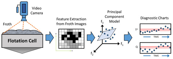
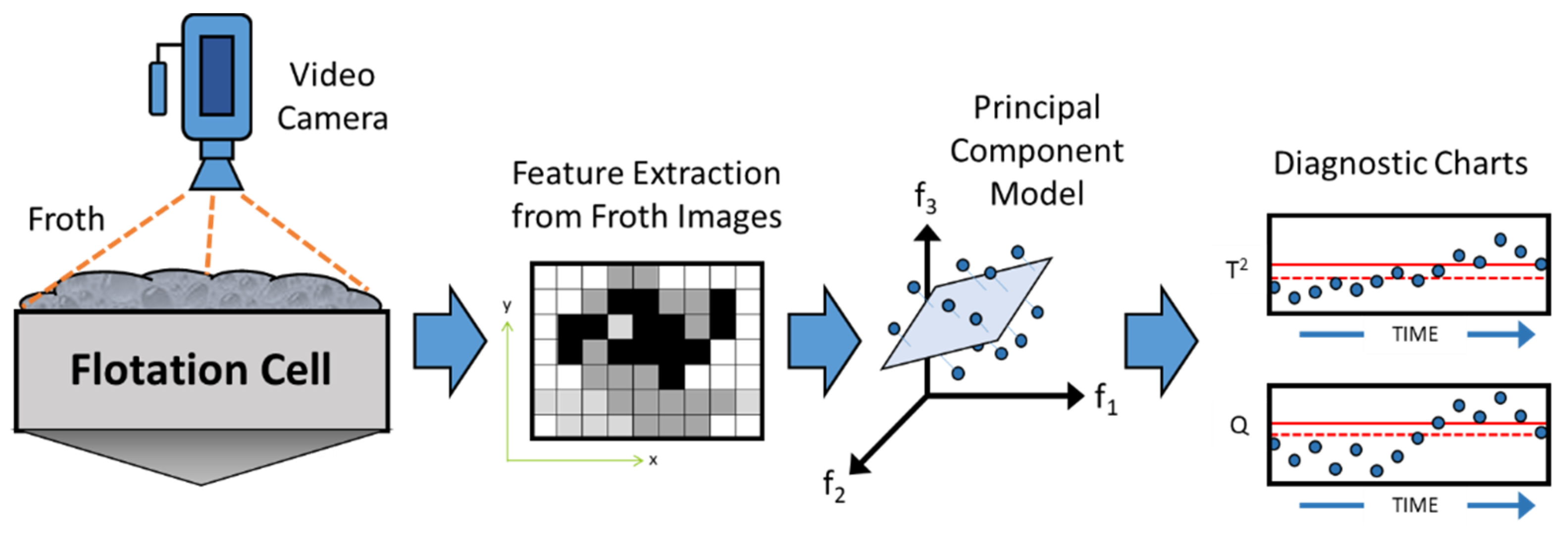
The monitoring strategy considered in this investigation is based on a traditional multivariate statistical process monitoring framework, with a principal component model. The principal component model is constructed from features extracted from images that represent normal process operation, as schematically illustrated in Figure 1.

Figure 1. Multivariate process monitoring based on flotation froth image analysis.

In essence, features extracted from the froth images are used to construct a principal component model that can generate monitoring diagnostics with which the in-control or out-of-control state of the process can be determined statistically.

Any of a number of different approaches can be followed to extract features from these images, and in this study, grey level co-occurrence matrices and local binary patterns are considered, as described in more detail in the following sections, followed by a discussion of the principal component model.

2.1. Feature Extraction with Grey Level Co-Occurrence Matrices

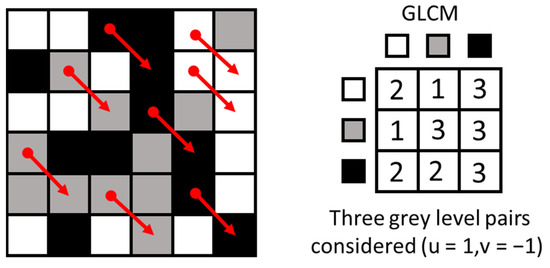
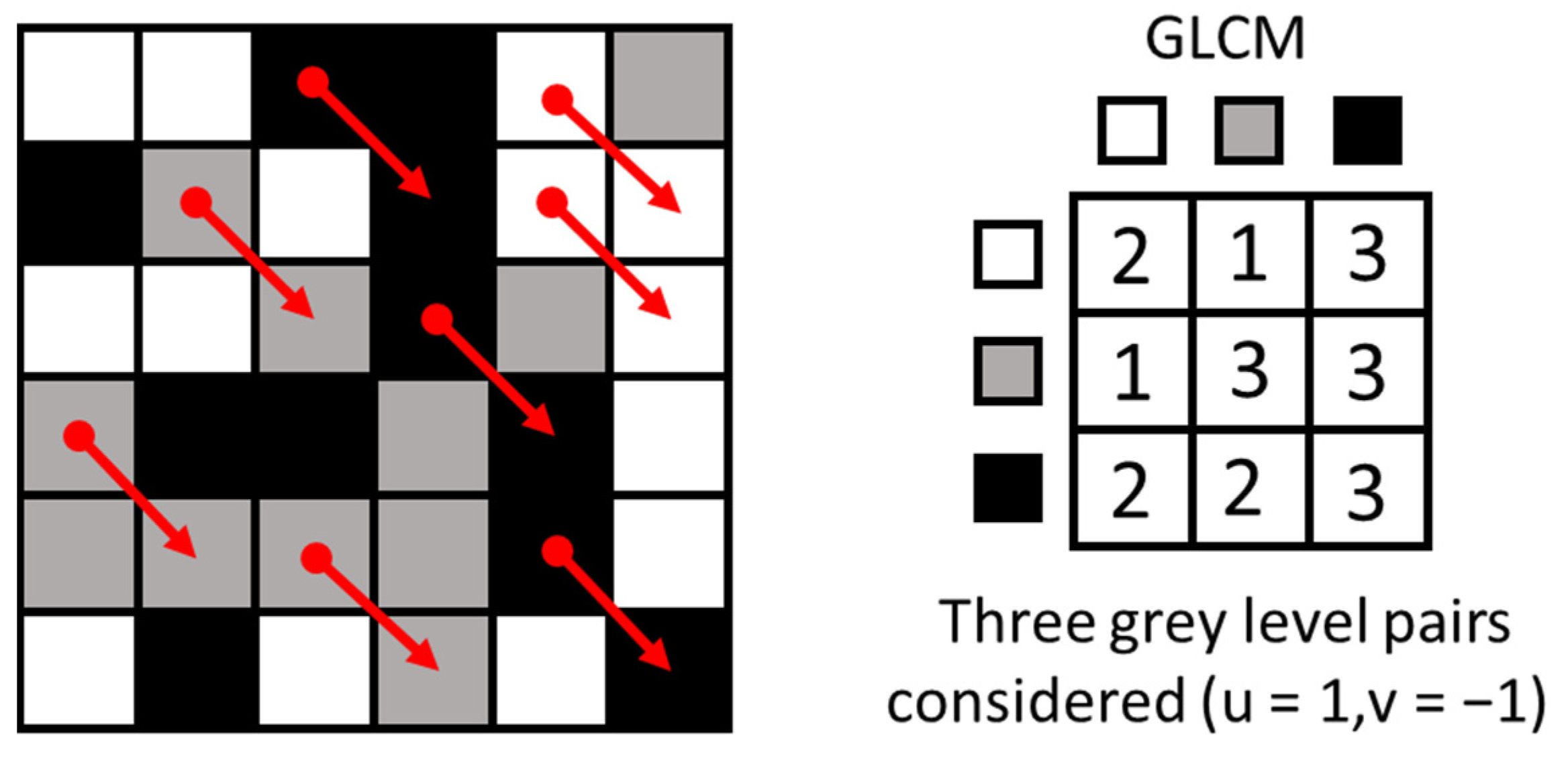
The grey level co-occurrence matrix is represented by $A_{I\left(D,G\right)}$ of an image $I$ with parameters $D$ and $G$, where $D$ is the distance between each pair of pixels in the image and $G$ is the number of grey levels considered in the image, as indicated in Figure 2. Each entry, $a_{ij}$, in the $\times G$ matrix denotes the number of times that a grey level is associated with a pair of pixels at displacement $D$ in the image.

Figure 2. A co-occurrence matrix shows the frequency of every particular pair of grey levels in pixel pairs, separated by a certain distance and direction, as specified by Cartesian coordinates (u,v).

The Haralick [33] set of image descriptors extracted from GLCM images are often used in image analysis. In this investigation, the following four features were used:

$$ENE={\displaystyle \sum }_{ij}{\check{a}}_{ij}^2$$

(1)

$$CON={\displaystyle \sum }_{ij}{\left|i-j\right|}^2{\check{a}}_{ij}$$

(2)

$$COR={\displaystyle \sum }_{ij}\frac{\left(i-m_i\right)\left(j-m_j\right){\check{a}}_{ij}}{s_i{s}_j}$$

(3)

$$HOM={\displaystyle \sum }_{ij}\frac{{\check{a}}_{ij}}{1+\left|i-j\right|}$$

(4)

In Equations (1)–(4), ${\check{a}}_{ij}$ is the (i,j)th element of the normalised GLCM and $m_k$ and $s_k$ are the mean and standard deviation of the matrix rows and columns. The energy (ENE) is a measure of the local uniformity of grey levels and large ENE values are associated with pixels that are very similar. The contrast (CON) is a measure of the intensity of grey level variations between neighbouring pixels, i.e., large CON values reflect large differences. The correlation (COR) represents the linear dependency between grey values in the co-occurrence matrix, while the homogeneity (HOM) shows the closeness of the distribution of elements in the co-occurrence matrix to its diagonal, i.e., HOM would approach unity when there are only a few dominant grey tones present. Homogeneity and contrast are typically inversely correlated.

GLCM methods were some of the very first to be used in froth image analysis [17,18,19] and have since been considered extensively in a range of applications in froth image analysis.

2.2. Feature Extraction with Local Binary Patterns

Applied on a pixel-by-pixel basis in images, local binary pattern operators compare the intensity of each pixel to the intensities of the other pixels in its neighbourhood [34]. The difference in the intensity between each neighbouring pixel $g_p$ and the centre pixel $g_c$ under consideration is thresholded by applying a binary thresholding function s:

$$\begin{array}{c}\mathrm{s}\left(g_p-g_c\right)=0\\ \mathrm{s}\left(g_p-g_c\right)=1\end{array}\},\mathrm{if}\begin{array}{c}{g}_c<g_p\\ g_c\ge g_p\end{array},\mathrm{for}\mathrm{all}p=1,2,\dots P$$

(5)

The local binary pattern (LBP) is subsequently computed as:

$$\mathrm{LBP}={\displaystyle \sum }_{p=1}^P{2}^p\mathrm{s}\left(g_p-g_c\right),\mathrm{for}\mathrm{all}p=1,2,\dots P$$

(6)

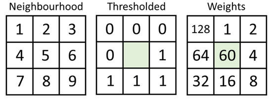
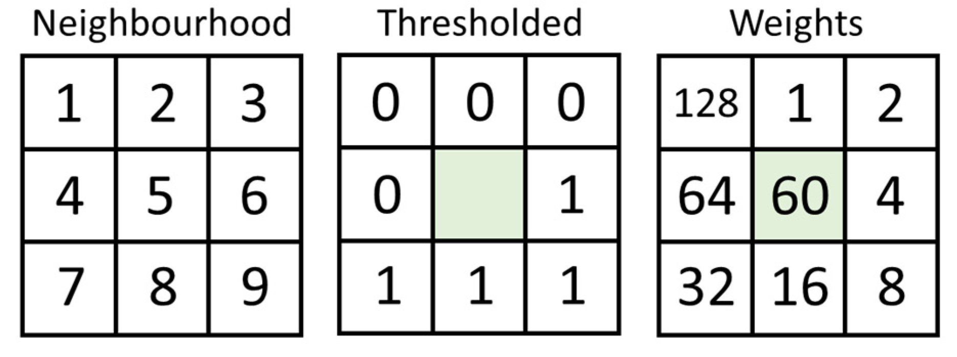
By applying the LBP operator to each pixel in an image with G grey levels, as indicated in Figure 3, the image is represented by LBPs ranging from 0 to G and these images are referred to as LBP images.

Figure 3. Example of a centre pixel (shaded), with its eight neighbouring pixels (left), the values obtained through binary thresholding (middle) and the conversion weights by which the thresholded val-ues are multiplied to give the decimal LBP value shown in place of the centre pixel (right).

LBP feature extraction has only relatively recently been considered in mineral processing [22,23,35].

2.3. Construction of Principal Component Models

Principal component analysis underpins traditional multivariate statistical process control. Essentially, the centred and scaled data matrix ($X$) that represents normal operating conditions (NOCs), consisting of $N$ samples of $M$ variables, $X\in {ℝ}^{N\times M}$ is expressed as the product of a score matrix ($T_K\in {ℝ}^{N\times M}$) and the transpose of a loading matrix ($P_K\in {ℝ}^{M\times K}$):

$$X=T_K{P}_K{}^{\prime }+E_K$$

(7)

The subscript $K$ denotes the number of principal components retained in the model, typically with $K\ll M$. $E_K\in {ℝ}^{N\times M}$ is a residual matrix resulting from the approximation of the data matrix with $K$ principal components. Specification of the hyperparameter K can be based on a number of statistical and heuristic methods. These include a value where the variance explained by the retained principal components would exceed a certain threshold (typically 80–90%), scree test, the Kaiser–Guttman test, partial correlation procedures, etc. [36,37]. In this investigation, crossvalidation was used to determine K.

The loading matrix $P$ is obtained by solving an eigenvalue problem, as represented by Equation (8):

$$\left(C-{\lambda }_{j}I\right)p_j=\mathbf{0}$$

(8)

In Equation (8), $C\in {ℝ}^{M\times M}$ is the covariance or correlation matrix of the variables, which are typically scaled to zero mean and unit variance, i.e.,

$$C=\frac{X^{\prime }X}{N-1}$$

(9)

Moreover, ${\lambda }_j$ is the j’th eigenvalue associated with the j’th principal component (j = 1, 2, … M) or loading vector ($p_j\in {ℝ}^{M\times 1}$).

In the traditional multivariate process control framework, the Hotelling T² and Q-statistics can be used to monitor operations. In the special case, where $K\le 3$, monitoring can be based on 2-D or 3-D score plots:

$$T_{i,K}^2={\displaystyle \sum }_{j=1}^K\frac{t_{ij}^2}{{\lambda }_j}$$

(10)

Hotelling’s T² statistic is calculated in accordance with Equation (10), where $t_{ij}$ is the score of the i’th sample on the j’th principal component (j = 1, 2, … K), and ${\lambda }_j$ is the eigenvalue associated with the j’th principal component. The Q-statistic is calculated according to Equation (11), where $e_{ij}$ is the residual of the i’th observation of the j’th feature when reconstructed with the first K principal components:

$$Q_{i,K}={\displaystyle \sum }_{j=1}^K{e}_{ij}^2$$

(11)

The 95% and 99% confidence limits on these charts are based on the 95th and 99th percentiles of the NOC data. New measurements above these control limits are considered out of control and would normally flag further diagnostic and corrective steps.

Application of the methodology is considered in the following two case studies.

3. Case Study 1: Monitoring of PGM Froths

The first case study is based on froth images obtained from a platinum metals group plant in South Africa. No other data regarding process conditions that are associated with the images have been recorded or are available, but even so, the data can serve as a basis for comparison of the different approaches.

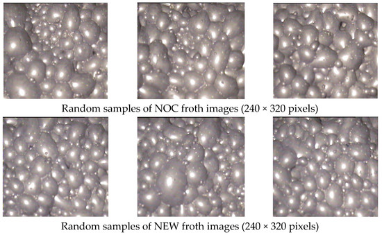
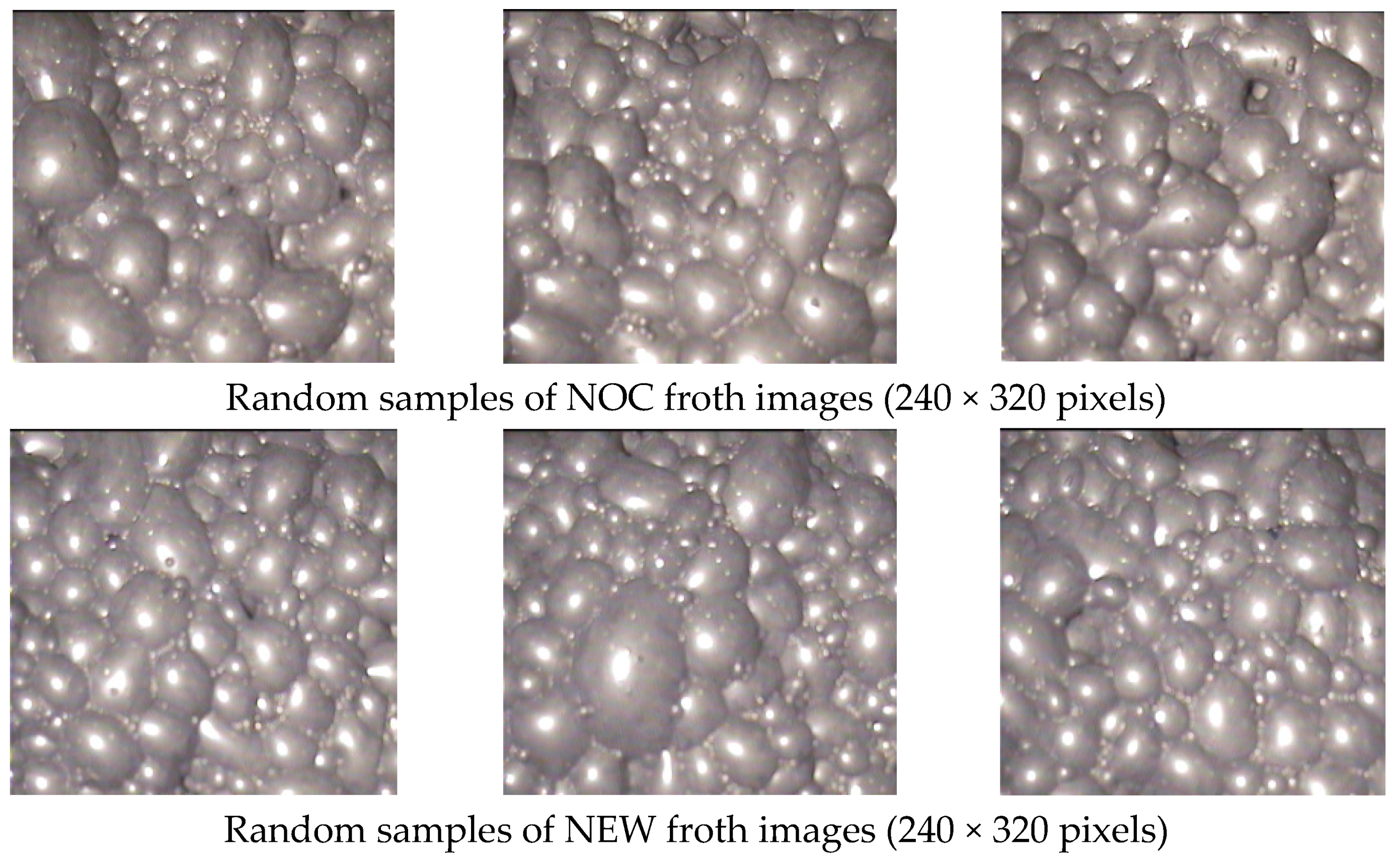
Three random examples of images representative of NOCs are shown in Figure 4 (top), while new images are shown in Figure 4 (bottom).

Figure 4. Images associated with NOCs (top, left to right) and test images (bottom, left to right).

The NOC image set contained 300 images, while the new data set contained 295 images, and these will be referred to as NEW images. As can be seen from Figure 4, it is difficult to visually discriminate between the NOCs and NEW images, as the bubble size distributions appear to be the same and colour cannot be used as a basis for discrimination either. This is a typical problem encountered by plant operators responsible for monitoring the flotation process and even if the plant is not monitored by means of a principal component model, as is considered in this investigation, visualization of the features extracted from the froths could provide very useful decision support for operators.

3.1. Monitoring Based on GLCM Features

Gray scale co-occurrence matrices were constructed based on the frequency with which a pixel with intensity value i occurred horizontally immediately adjacent to a pixel with intensity value j, i.e., [0 1] in Cartesian coordinates. After optimization over the range G = [2 64], eight grey levels were used, as these gave the best results. Even so, across the range, these G levels did not have a particularly strong effect on the overall performance of the monitoring methodology.

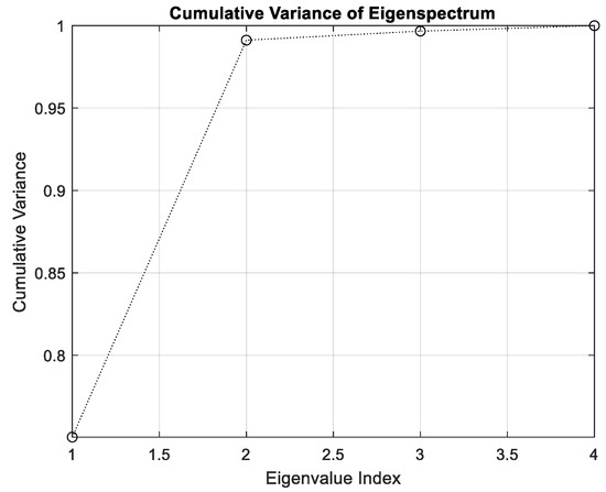
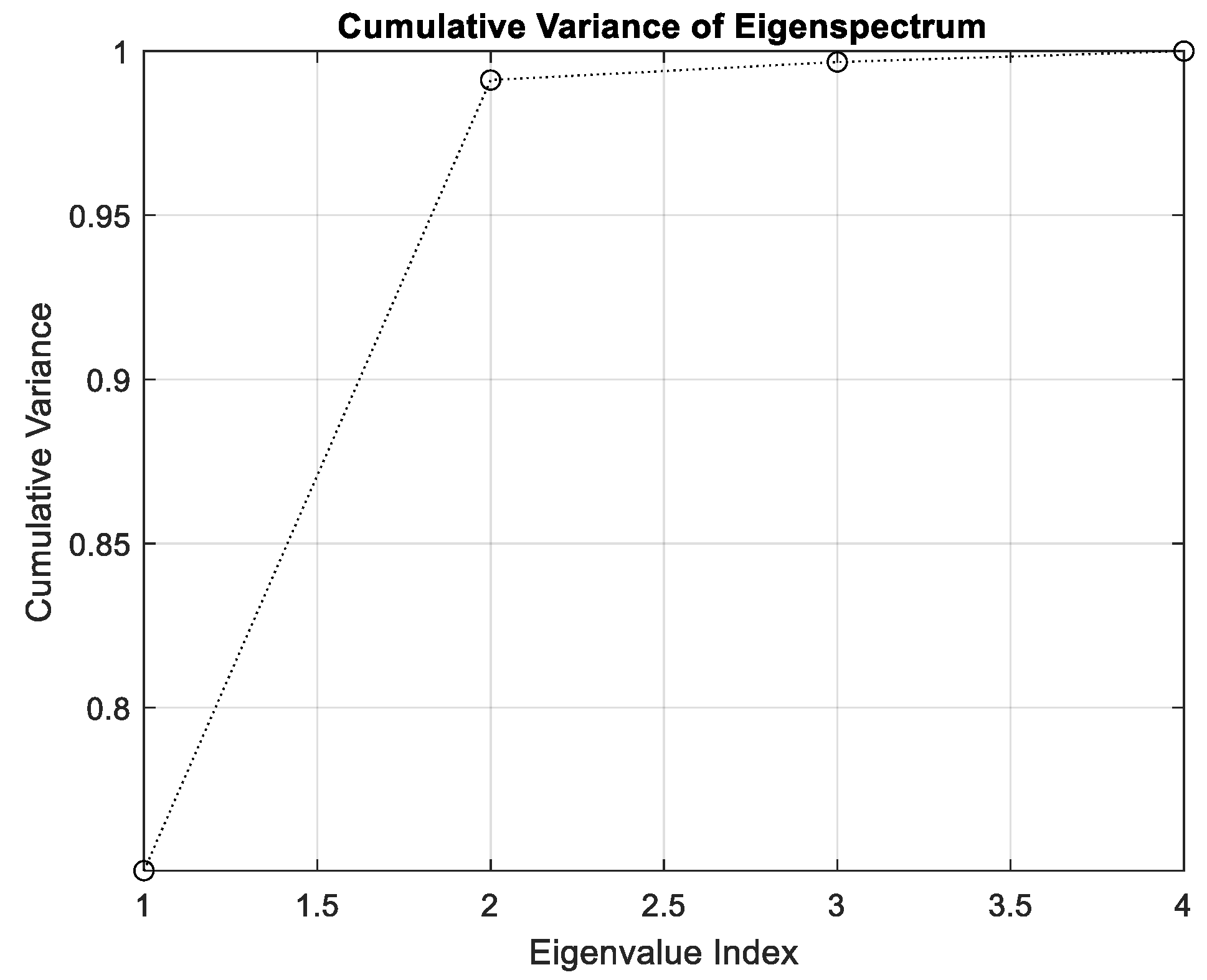
The eigenspectrum of the principal component model based on the four GLCM features is shown in Figure 5. As can be seen from this figure, the first two principal components essentially captured all the variation in the features and hence K = 2 components were retained, which was also indicated by a cross-validation approach.

Figure 5. Cumulative eigenvalue plot of GLCM features in case study 1.

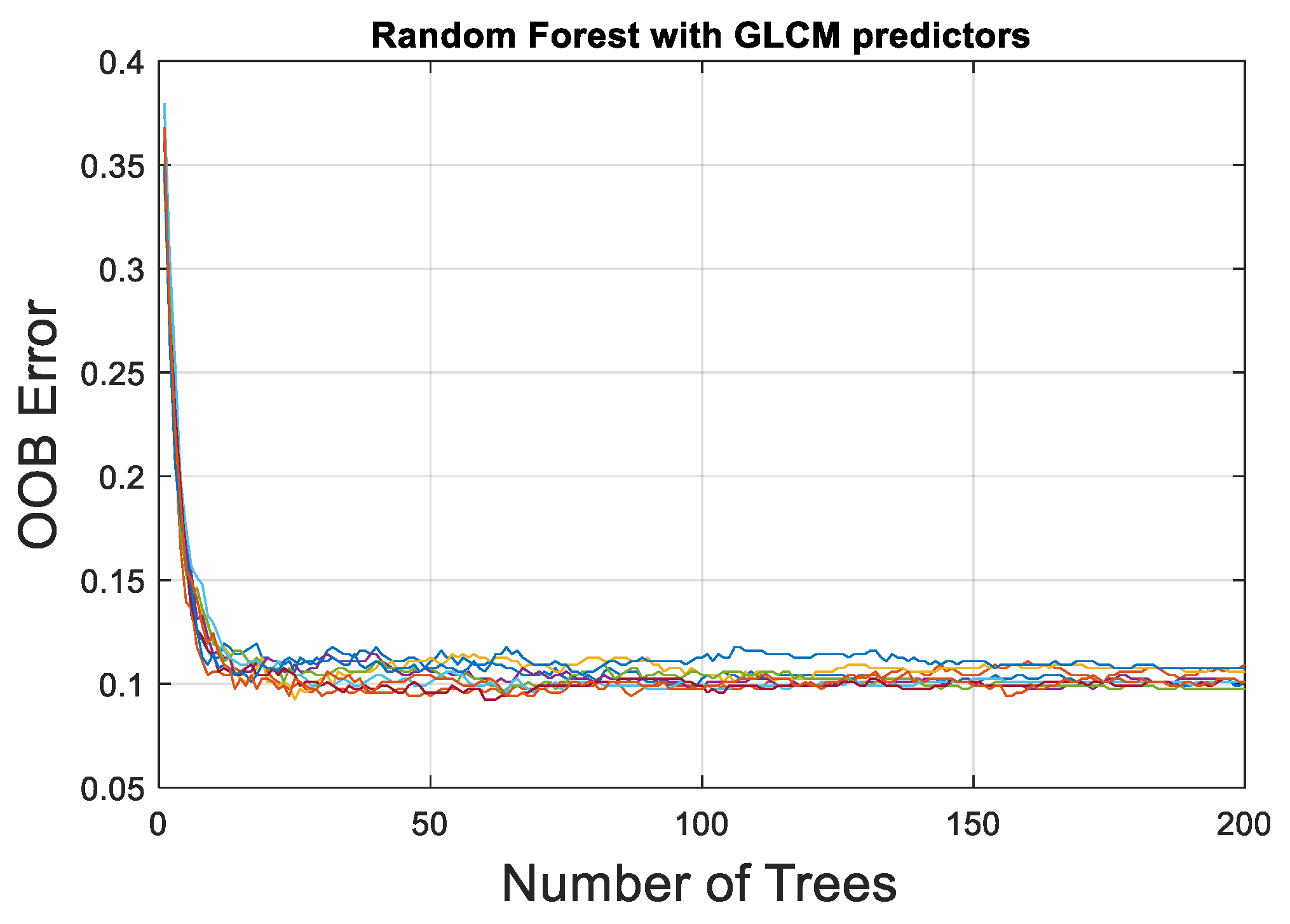
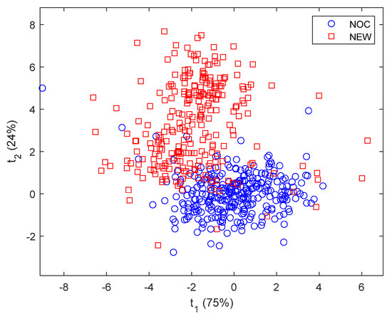
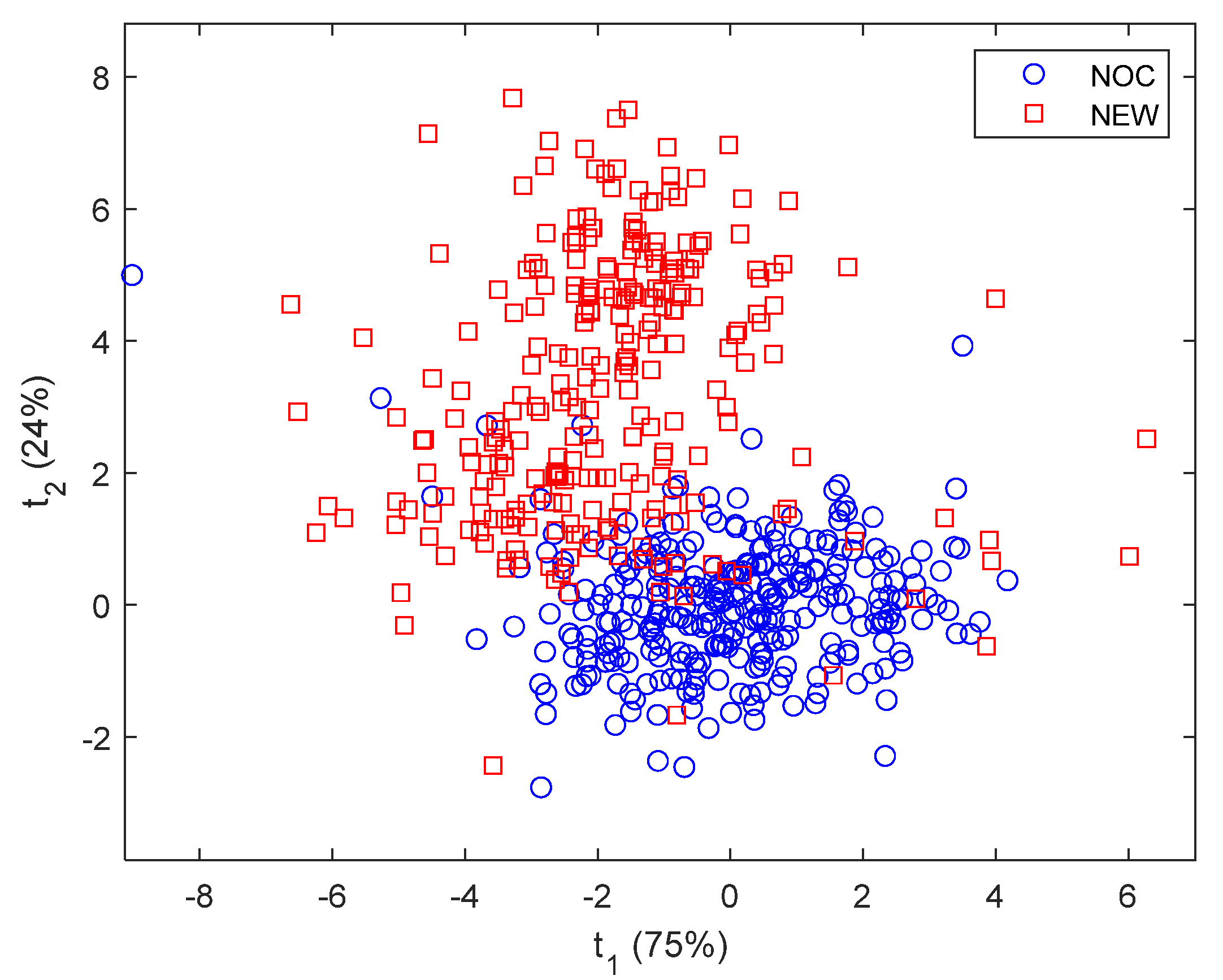
Figure 6 is a bivariate scatterplot of the principal component scores of the GLCM features for the NOC and NEW data. These data sets are well separated in the figure. This separation could be further quantified by using a random forest model with the four GLCM features as predictors to classify the data as either NOC or NEW. The random forest could do so with an out-of-bag error of approximately 9%, as indicated in Appendix A.

Figure 6. Principal component score plot of four GLCM features with 8 grey levels in case study 1. Blue circles and red squares indicate NOC and NEW data, respectively.

Plots such as these could be used as a complementary means to track the flotation process, given that each marker in Figure 6 represents a froth image. This could serve as an aid to operators in steering the flotation process.

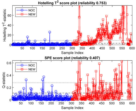
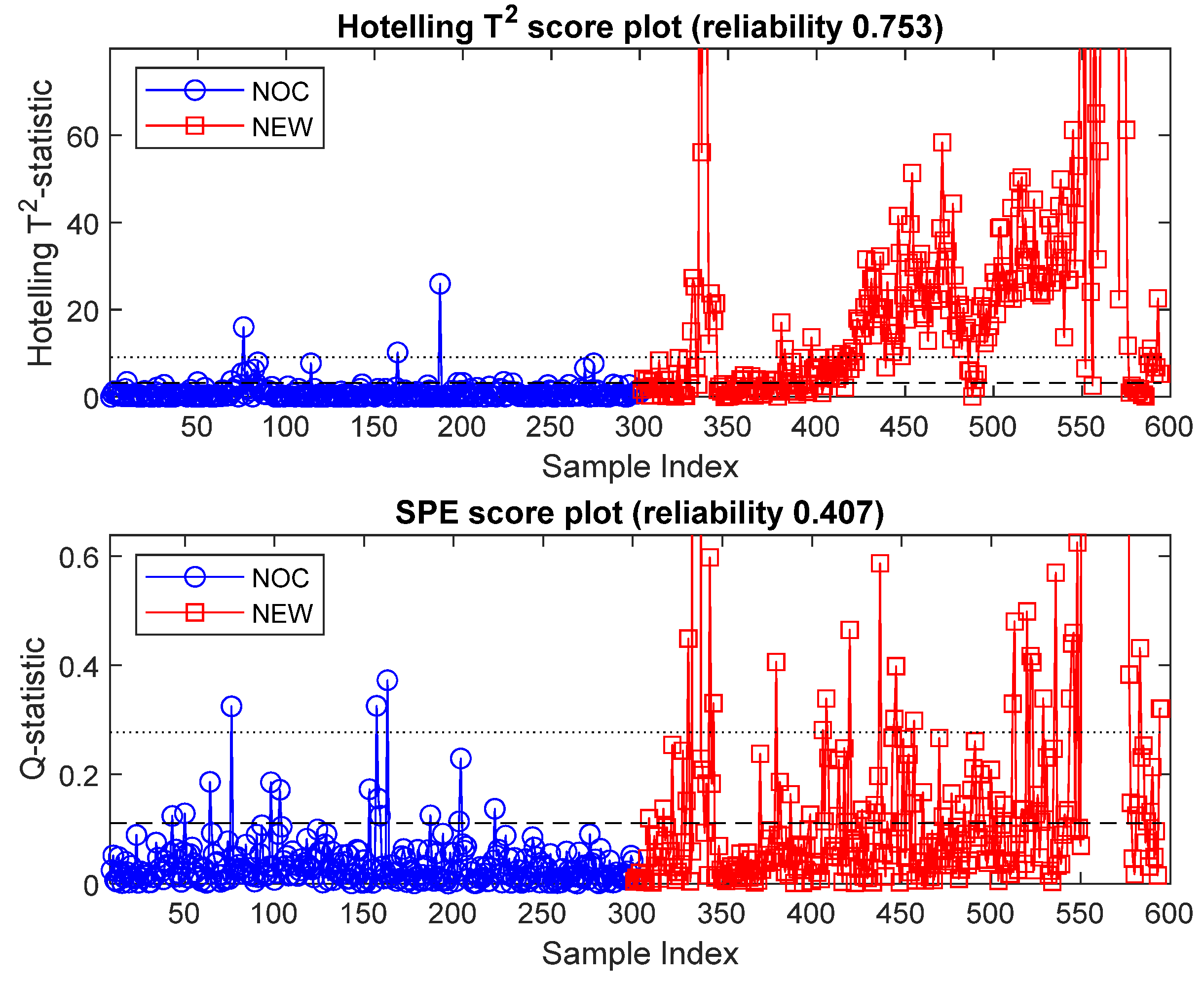
Although the principal component model consisted of two components only, the Hotelling’s T² and Q-statistics are still presented as a more general basis for monitoring purposes. These charts are shown in Figure 7 and show that approximately 75.3% of the new data could be flagged as out of control.

Figure 7. Hotelling’s T² (top) and Q-chart (bottom) of GLCM features in case study 1. The 95% and 99% confidence limits are indicated by dashed and dotted lines in each plot.

3.2. Monitoring Based on LBP Features

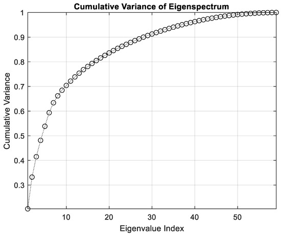
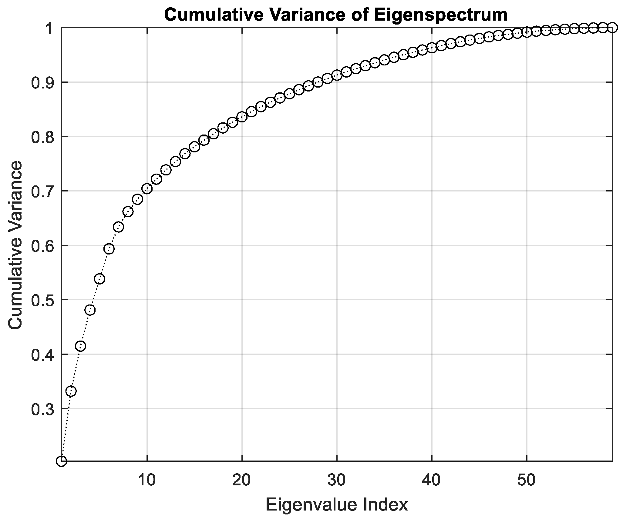
The optimal LBP features were obtained with a neighbourhood of 2 and 59 features were extracted. The eigenspectrum of the principal components of these features is shown in Figure 8. K = 3 principal components were retained in the model, as determined by cross-validation. This value is of necessity comparatively low, owing to the comparatively small size of the NOC data set in relation to the number of features.

Figure 8. Eigenspectrum of the LBP features of the NOCs froth images in case study 1.

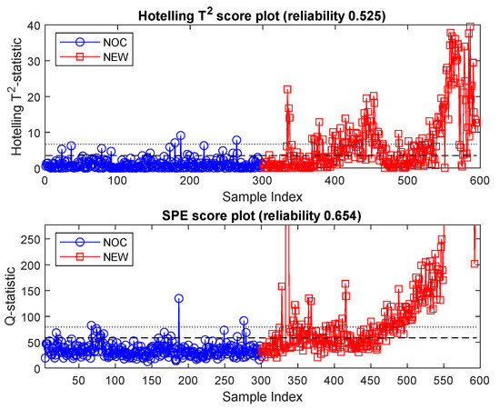
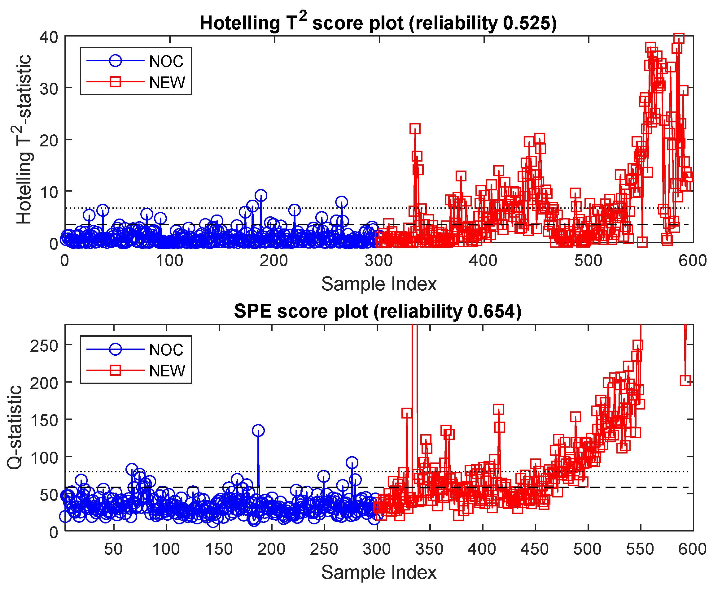
The diagnostic charts generated by the principal component model are shown in Figure 9. Interestingly, the LBP feature set could flag approximately 65.4% of the NEW data as out of control at a 95% confidence level.

Figure 9. The Hotelling T² (top) and Q-chart (bottom) showing NOCs and new data, based on the use of LBP features. The 95% and 99% confidence limits are indicated by dashed and dotted lines in each plot.

4. Case Study 2: Monitoring of Platinum Froths Associated with Different Grades

In the second case study, the froth image database previously considered by Marais and Aldrich [38], as well as Horn et al. [39], was revisited. The image data were originally collected over a four-hour period on a primary cleaner cell on a South African industrial PGM plant. During collection of the images, the air flow rate of the cell was periodically varied. Concentrate samples were collected after stabilization of the flotation cell and afterwards, the PGM content was analysed in a laboratory.

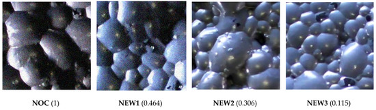
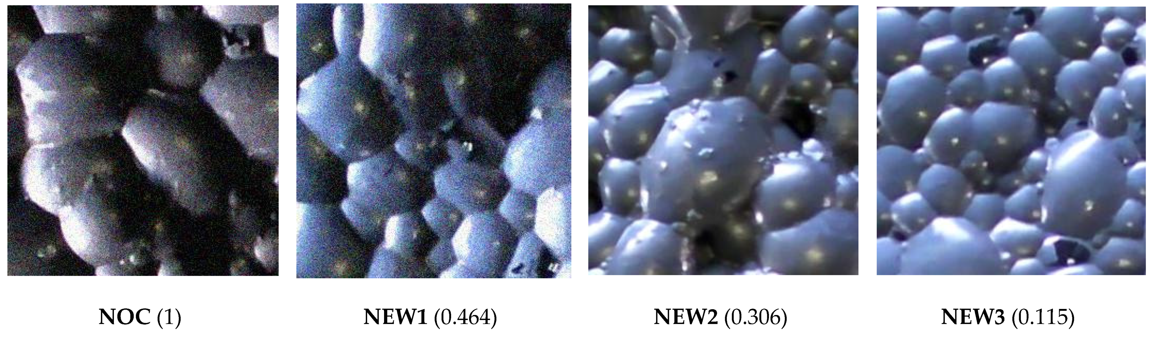
The 256 × 256 pixel images represent four different operational regimes with relative platinum grades of 1, 0.464, 0.306, and 0.115, as indicated in Figure 9.

The NOC image set consisted of froth images associated with a high grade of platinum, while the NEW1, NEW2, and NEW3 data sets consisted of froth images with progressively lower grades. Figure 10 shows a typical example of an image of each regime. As before, features were extracted from all the images, while the principal component model was based on NOC data only.

Figure 10. Images associated with NOC and NEW1, NEW2, and NEW3 operational regimes in case study 2. Relative platinum grades are indicated in parentheses.

4.1. Monitoring Based on GLCM Features

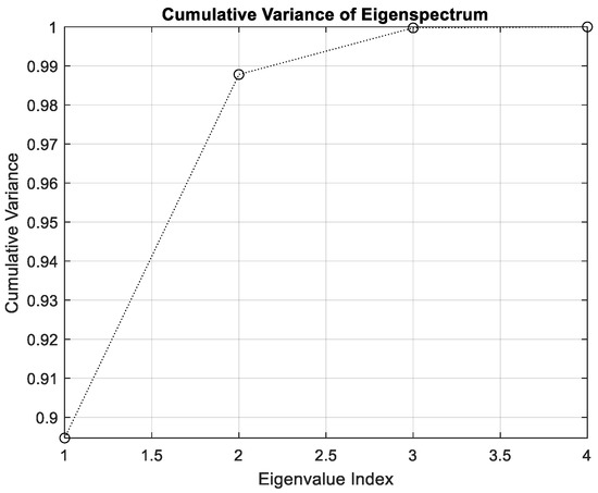
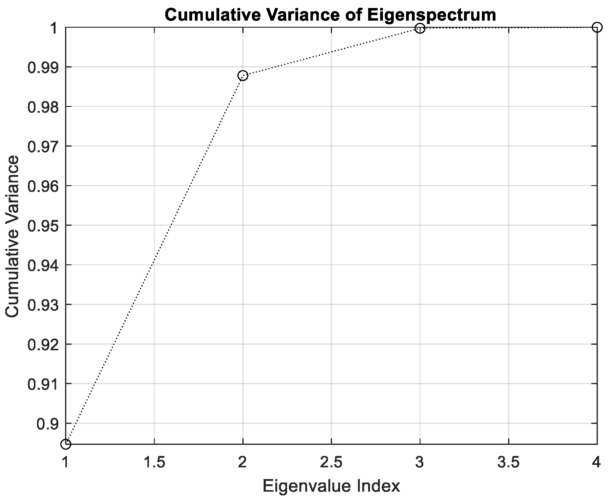
As before, four GLCM features were extracted from the images based on the use of G = 8 grey levels and a horizontal distance of 1 between pixels. The eigenspectrum of the extracted features is shown in Figure 11.

Figure 11. Eigenspectrum of the GLCM features of the NOC froth images in case study 2.

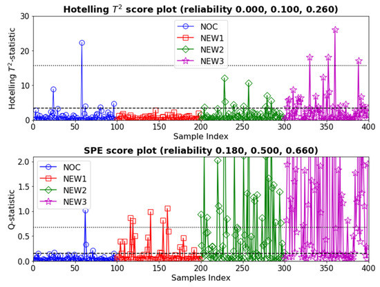
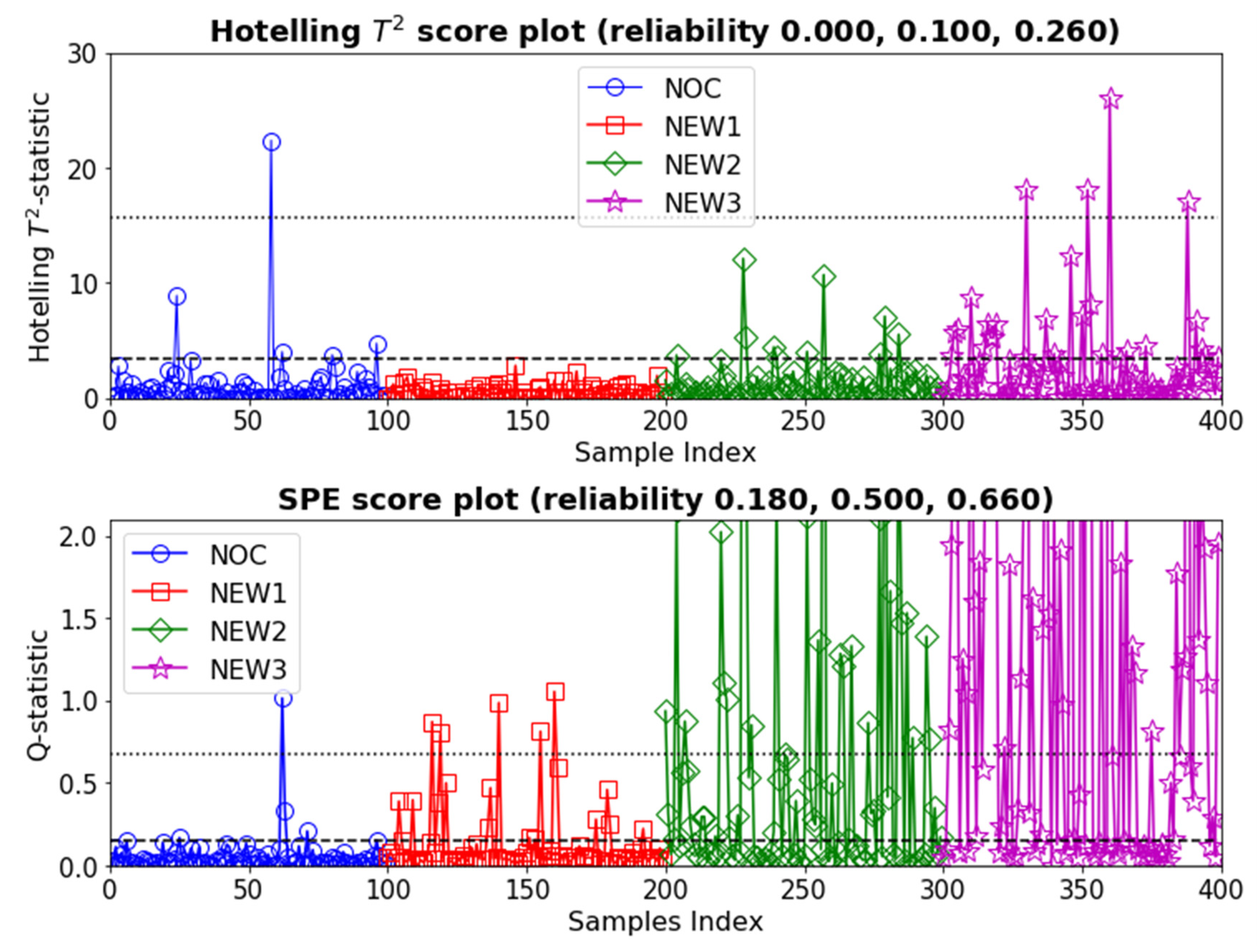
With these features, the principal component model could flag approximately 44.7% of the new data as out of control, i.e., 18%, 50%, and 66% of the NEW1, NEW2, and NEW3 data, respectively, as indicated in Figure 12.

Figure 12. The Hotelling T² (top) and Q-chart (bottom) showing NOCs and new data (NEW1 with indices from 101 to 200, NEW2 with indices from 201 to 300 and NEW3 with indices from 301 to 400), based on the use of GLCM features in case study 2. The 95% and 99% confidence limits are indicated by dashed and dotted lines in each plot.

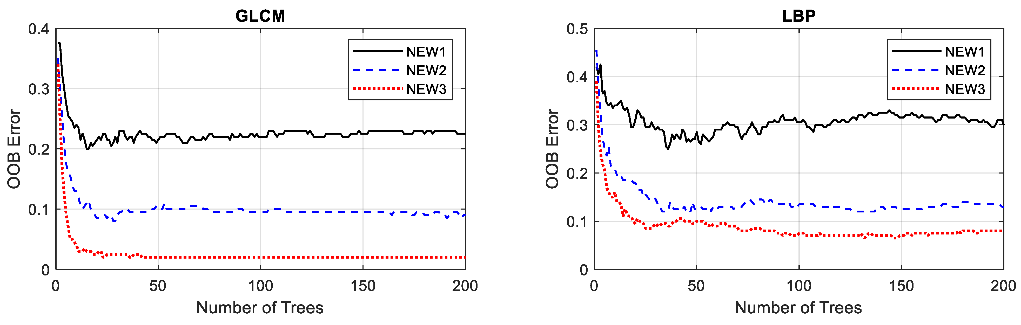
To put this in perspective, a random forest model (Appendix A) using the GLCM features as predictors could discriminate between the NOCs data and the NEW1, NEW2, and NEW3 data respectively with accuracies of approximately 77%, 92%, and 98%.

4.2. Monitoring Based on LBP Vectors

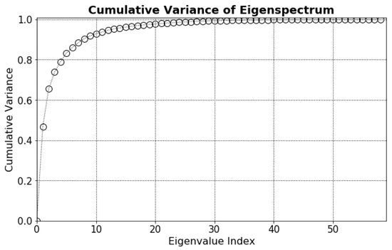
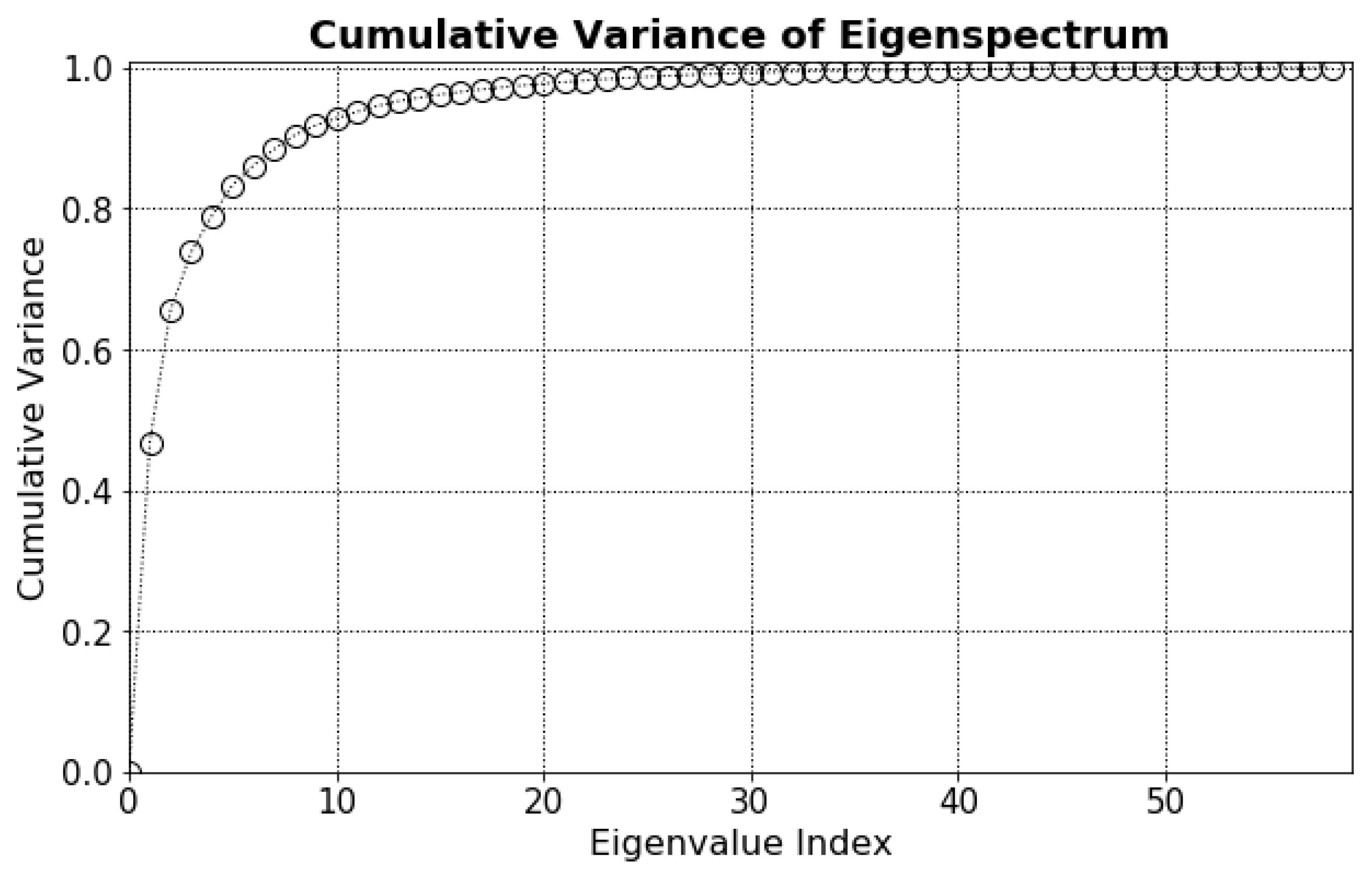
Monitoring of the process was again based on 59 LBP vectors extracted from the images. K = 3 principal components were retained, the cumulative eigenspectrum of which is shown in Figure 13.

Figure 13. Cumulative eigenspectrum of the principal component model based on the retention of 3 of 59 LBP features in case study 2.

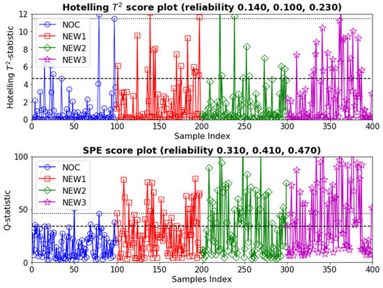
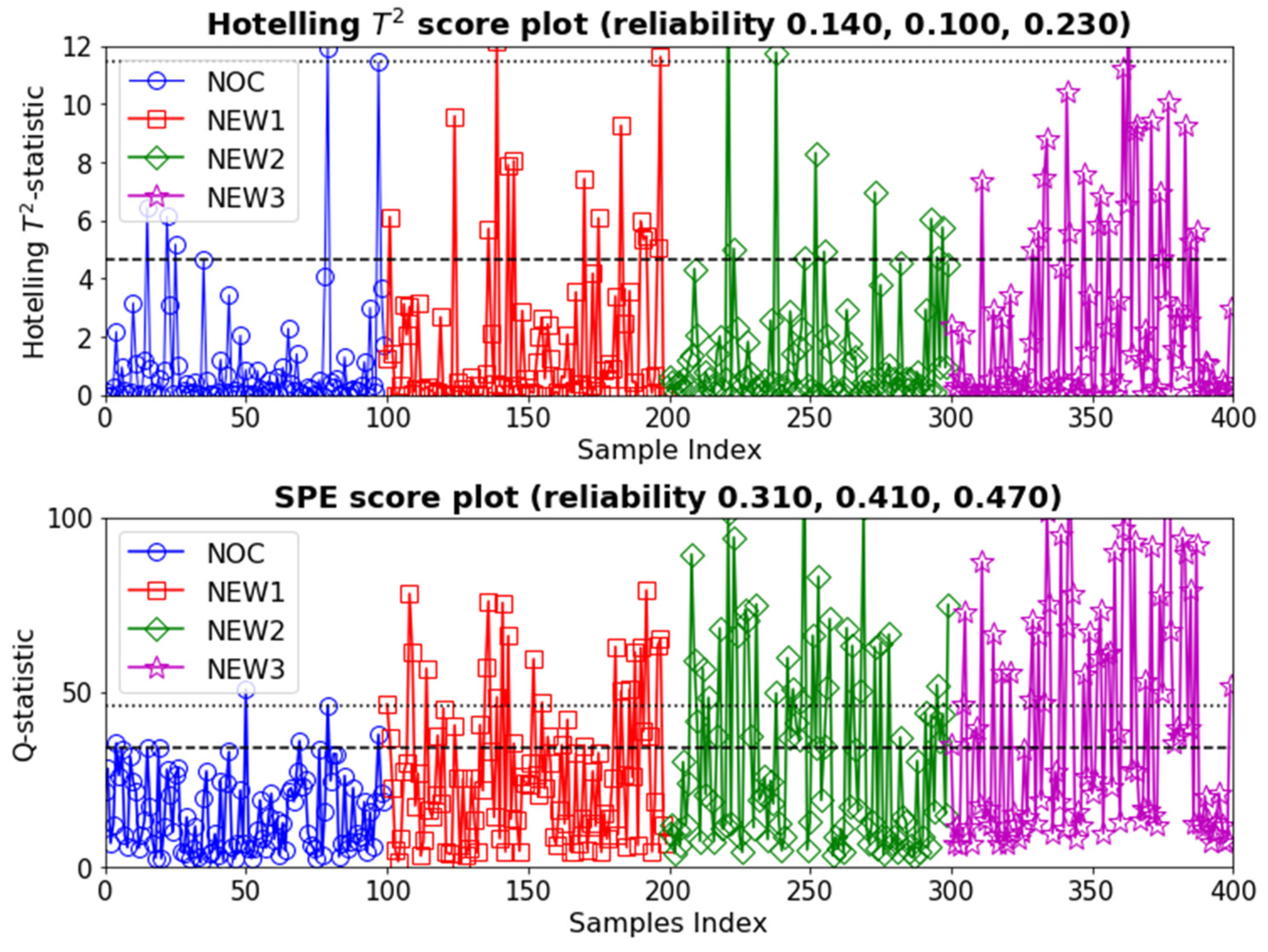
The diagnostic charts are shown in Figure 14. As can be seen from the Q-chart at the bottom of Figure 14, the model could identify NEW1, NEW2, and NEW3 process deviations with a reliability of 31%, 41%, and 47%. This could be compared with the ability of a random forest model (Appendix A) using the 59 LBP features as predictors to discriminate between the NOC data and the NEW1, NEW2, and NEW2 data, which was approximately 79%, 90%, and 98%. This was essentially the same as what could be obtained with the GLCM features.

Figure 14. Hotelling’s T² chart (top) and Q-chart (bottom) showing the NOCs (blue), NEW1 (red), NEW2 (green) and NEW3 (magenta) data for local binary patterns in case study 2. The 95% and 99% confidence limits are indicated by dashed and dotted lines in each plot.

5. Discussion and Conclusions

In this paper, it was shown that features extracted from froth images representative of normal operating conditions (NOCs) could be used in a traditional multivariate statistical process control framework, such as being based on the use of principal component analysis.

To this end, the physical interpretation of the features was not important, although it would be possible to link some of these features to the physical characteristics of the froth, such as the bubble size and shape distributions and the appearance of the froth in general. Such an analysis would also have to consider changes in the froth structures over time.

Both algorithms that were used to extract features from the images performed reasonably well, despite the wide disparity in the number of features that were used to characterize the froth images. Nonetheless, there appeared to be considerable scope for improvement. First, it should be noted that the small sizes of the NOCs image data sets placed significant constraints on the use of some of the state-of-the-art approaches to image analysis, particularly methods based on deep learning, such as those considered by Fu and Aldrich [40,41] for example. Larger NOCs data sets would therefore need to be considered in future studies.

In addition, extension of the linear principal component model to any number of nonlinear versions could also lead to potentially considerable improvement in the results.

Finally, if these image features are used in combination with other process variables, further diagnostic methods would add critical additional functionality to the model and could be readily incorporated into the model. In practice, this would be important in order to steer an out-of-control process back to an in-control state.

References

- Neethling, S.J.; Brito-Parada, P.R. Predicting flotation behaviour—The interaction between froth stability and performance. Miner. Eng. 2018, 120, 60–65. [Google Scholar] [CrossRef] [Scilit]
- Farrokhpay, S. The significance of froth stability in mineral flotation—A review. Adv. Colloid Interface Sci. 2011, 166, 1–7. [Google Scholar] [CrossRef] [Scilit]
- Cutting, G.W.; Barber, S.P.; Newton, S. Effects of froth structure and mobility on the performance and simulation of continuously operated flotation cells. Int. J. Miner. Process. 1986, 16, 43–61. [Google Scholar] [CrossRef] [Scilit]
- Ni, C.; Bu, X.; Xia, W.; Liu, B.; Peng, Y.; Xie, G. Improving lignite flotation performance by enhancing the froth properties using polyoxyethylene sorbitan monostearate. Int. J. Miner. Process. 2016, 155, 99–105. [Google Scholar] [CrossRef] [Scilit]
- Sheni, N.; Corin, K.; Wiese, J. Considering the effect of pulp chemistry during flotation on froth stability. Miner. Eng. 2018, 116, 15–23. [Google Scholar] [CrossRef] [Scilit]
- Ng, C.Y.; Park, H.; Wang, L. Improvement of coal flotation by exposure of the froth to acoustic sound. Miner. Eng. 2021, 168, 106920. [Google Scholar] [CrossRef] [Scilit]
- Mesa, D.; Morrison, A.J.; Brito-Parada, P.R. The effect of impeller-stator design on bubble size: Implications for froth stability and flotation performance. Miner. Eng. 2020, 157, 106533. [Google Scholar] [CrossRef] [Scilit]
- Nuorivaara, T.; Serna-Guerrero, R. Unlocking the potential of sustainable chemicals in mineral processing: Improving sphalerite flotation using amphiphilic cellulose and frother mixtures. J. Clean. Prod. 2020, 261, 121143. [Google Scholar] [CrossRef] [Scilit]
- Tsatouhas, G.; Grano, S.R.; Vera, M. Case studies on the performance and characterisation of the froth phase in industrial flotation circuits. Miner. Eng. 2006, 19, 774–783. [Google Scholar] [CrossRef] [Scilit]
- Quintanilla, P.; Neethling, S.J.; Brito-Parada, P.R. Modelling for froth flotation control: A review. Miner. Eng. 2021, 162, 106718. [Google Scholar] [CrossRef] [Scilit]
- Ai, M.; Xie, Y.; Xie, S.; Gui, W. Shape-weighted bubble size distribution based reagent predictive control for the antimony flotation process. Chemom. Intell. Lab. Syst. 2019, 192, 103821. [Google Scholar] [CrossRef] [Scilit]
- Zhang, L.; Xu, D. Flotation bubble size distribution detection based on semantic segmentation. IFAC Pap. 2020, 53, 11842–11847. [Google Scholar] [CrossRef] [Scilit]
- Zhang, H.; Tang, Z.; Xie, Y.; Gao, X.; Chen, Q. A watershed segmentation algorithm based on an optimal marker for bubble size measurement. Measurement 2019, 138, 182–193. [Google Scholar] [CrossRef] [Scilit]
- Zhao, L.; Peng, T.; Xie, Y.; Yang, C.; Gui, W. Recognition of flooding and sinking conditions in flotation process using soft measurement of froth surface level and QTA. Chemom. Intell. Lab. Syst. 2017, 169, 45–52. [Google Scholar] [CrossRef] [Scilit]
- He, Z.; Tang, Z.; Yan, Z.; Liu, J. DTCWT-based zinc fast roughing working condition identification. Chin. J. Chem. Eng. 2018, 26, 1721–1726. [Google Scholar] [CrossRef] [Scilit]
- Ming, L.; Wei-hua, G.; Tao, P.; Wei, C. Fault condition detection for a copper flotation process based on a wavelet multi-scale binary froth image. Rem Rev. Esc. Minas 2015, 68, 177–185. [Google Scholar] [CrossRef] [Scilit]
- Moolman, D.W.; Aldrich, C.; Van Deventer, J.S.J.; Stange, W.W. Digital image processing as a tool for on-line monitoring of froth in flotation plants. Miner. Eng. 1994, 7, 1149–1164. [Google Scholar] [CrossRef] [Scilit]
- Moolman, D.W.; Aldrich, C.; Van Deventer, J.S.J.; Bradshaw, D.J. The interpretation of flotation froth surfaces by using digital image analysis and neural networks. Chem. Eng. Sci. 1995, 50, 3501–3513. [Google Scholar] [CrossRef] [Scilit]
- Moolman, D.W.; Aldrich, C.; van Deventer, J.S.J. The monitoring of froth surfaces on industrial flotation plants using connectionist image processing techniques. Miner. Eng. 1995, 8, 23–30. [Google Scholar] [CrossRef] [Scilit]
- Zhao, L.; Peng, T.; Han, H.; Cao, W.; Lou, Y.; Xie, X. Fault condition recognition based on multi-scale co-occurrence matrix for copper flotation process. IFAC Proc. Vol. 2014, 47, 7091–7097. [Google Scholar] [CrossRef] [Scilit]
- Zhang, J.; Tang, Z.; Liu, J.; Tan, Z.; Xu, P. Recognition of flotation working conditions through froth image statistical modeling for performance monitoring. Miner. Eng. 2016, 86, 116–129. [Google Scholar] [CrossRef] [Scilit]
- Fu, Y.; Aldrich, C. Flotation froth image analysis by use of a dynamic feature extraction algorithm. IFAC Pap. 2016, 49, 84–89. [Google Scholar] [CrossRef] [Scilit]
- Aldrich, C.; Smith, L.K.; Verrelli, D.I.; Bruckard, W.J.; Kistner, M. Multivariate image analysis of realgar–orpiment flotation froths. Miner. Process. Extr. Metall. 2017, 127, 146–156. [Google Scholar] [CrossRef] [Scilit]
- Luo, J.; Tang, Z.; Zhang, H.; Fan, Y.; Xie, Y. LTGH: A dynamic texture feature for working condition recognition in the froth flotation. IEEE Trans. Instrum. Meas. 2021, 70, 1–10. [Google Scholar]
- Tan, J.; Liang, L.; Peng, Y.; Xie, G. The concentrate ash content analysis of coal flotation based on froth images. Miner. Eng. 2016, 92, 9–20. [Google Scholar] [CrossRef] [Scilit]
- Xu, D.; Chen, X.; Xie, Y.; Yang, C.; Gui, W. Complex networks-based texture extraction and classification method for mineral flotation froth images. Miner. Eng. 2015, 83, 105–116. [Google Scholar] [CrossRef] [Scilit]
- Aldrich, C.; Marais, C.; Shean, B.J.; Cilliers, J.J. Online monitoring and control of froth flotation systems with machine vision: A review. Int. J. Miner. Process. 2010, 96, 1–13. [Google Scholar] [CrossRef] [Scilit]
- Ai, M.; Xie, Y.; Xu, D. Reagent predictive control using joint froth image feature for antimony flotation process. IFAC Pap. 2018, 51, 284–289. [Google Scholar] [CrossRef] [Scilit]
- Lyu, Y.; Chen, J.; Song, Z. Image-based process monitoring using deep learning framework. Chemom. Intell. Lab. Syst. 2019, 189, 8–17. [Google Scholar] [CrossRef] [Scilit]
- Liu, J.J.; MacGregor, J.F.; Duchesne, C.; Bartolacci, G. Flotation froth monitoring using multiresolutional multivariate image analysis. Miner. Eng. 2005, 18, 65–76. [Google Scholar] [CrossRef] [Scilit]
- MacGregor, J.F.; Kourti, T.; Liu, J.; Bradley, J.; Dunn, K.; Yu, H. Multivariate methods for the analysis of data-bases, Process monitoring, and control in the material processing industries. IFAC Proc. Vol. 2007, 40, 193–198. [Google Scholar] [CrossRef] [Scilit]
- Zhang, H.; Tang, Z.; Xie, Y.; Gao, X.; Chen, Q.; Gui, W. Long short-term memory-based grade monitoring in froth flotation using a froth video sequence. Miner. Eng. 2021, 160, 106677. [Google Scholar] [CrossRef] [Scilit]
- Haralick, R.M.; Shanmugam, K.; Dinstein, I.H. Textural features for image classification. IEEE Trans. Syst. Man Cybern. 1973, SMC-3, 610–621. [Google Scholar] [CrossRef] [Scilit]
- Ojala, T.; Pietikäinen, M.; Harwood, D. A comparative study of texture measures with classification based on featured distributions. Pattern Recognit. 1996, 29, 51–59. [Google Scholar] [CrossRef] [Scilit]
- Kistner, M.; Jemwa, G.T.; Aldrich, C. Monitoring of mineral processing systems by using textural image analysis. Miner. Eng. 2013, 52, 169–177. [Google Scholar] [CrossRef] [Scilit]
- Hubbard, R.; Allen, S.J. An empirical comparison of alternative methods for principal component extraction. J. Bus. Res. 1987, 15, 173–190. [Google Scholar] [CrossRef] [Scilit]
- Jackson, J.E. A User’s Guide to Principal Components; Jackson, J.E., Ed.; Wiley John and Sons: New York, NY, USA, 1991. [Google Scholar]
- Marais, C.; Aldrich, C. Estimation of platinum flotation grades from froth image data. Miner. Eng. 2011, 24, 433–441. [Google Scholar] [CrossRef] [Scilit]
- Horn, Z.C.; Auret, L.; McCoy, J.T.; Aldrich, C.; Herbst, B.M. Performance of convolutional neural networks for feature extraction in froth flotation sensing. IFAC Pap. 2017, 50, 13–18. [Google Scholar] [CrossRef] [Scilit]
- Fu, Y.; Aldrich, C. Froth image analysis by use of transfer learning and convolutional neural networks. Miner. Eng. 2018, 115, 68–78. [Google Scholar] [CrossRef] [Scilit]
- Fu, Y.; Aldrich, C. Flotation froth image recognition with convolutional neural networks. Miner. Eng. 2019, 132, 183–190. [Google Scholar] [CrossRef] [Scilit]
Publisher’s Note: MDPI stays neutral with regard to jurisdictional claims in published maps and institutional affiliations. |
© 2021 by the authors. Licensee MDPI, Basel, Switzerland. This article is an open access article distributed under the terms and conditions of the Creative Commons Attribution (CC BY) license (https://creativecommons.org/licenses/by/4.0/).