


Abstract
Singularly perturbed integro-partial differential equations with reaction–diffusion behavior present significant challenges due to boundary layers arising from small perturbation parameters, which complicate the development of accurate and efficient numerical schemes for physical and engineering models. In this study, a uniformly convergent higher-order method is proposed to address these challenges. The approach applies the implicit Euler method for temporal discretization on a uniform mesh and central differences on a Shishkin mesh for spatial approximation, and utilizes the trapezoidal rule for evaluating integral terms; further, extrapolation techniques are incorporated in both time and space to increase accuracy. Numerical analysis demonstrates that the base scheme achieves first-order convergence, while extrapolation enhances convergence rates to second-order in time and fourth-order in space. Theoretical results confirm uniform convergence with respect to the perturbation parameter, and comprehensive numerical experiments validate these analytical claims. Findings indicate that the proposed scheme is reliable, efficient, and particularly effective in attaining fourth-order spatial accuracy when solving singularly perturbed integro-partial differential equations of reaction–diffusion type, thus providing a robust numerical tool for complex applications in science and engineering.
1. Introduction
The following integro-parabolic reaction–diffusion problem involving a small parameter at the highest derivative with initial and Dirichlet boundary conditions is considered:
where
Here, and . The functions on and , possess adequate smoothness and boundedness, and fulfill , and is the kernel function. Because the perturbation parameter is present in (1), the same old numerical strategies on a uniform mesh fail to yield accurate results for problem (1) [1]. To address this issue, the use of nonuniform meshes has been proposed, as discussed in [2]. Various numerical methods, including the finite element method (FEM), have been explored; see [3,4,5,6,7,8] for reference. Recently, Lange and Smith [9] established the existence and uniqueness of solutions for singularly perturbed Fredholm integro-ordinary differential equations (SPFIODEs). Sevgin [10] investigated a numerical method for nonlinear first-order singularly perturbed integro-differential equations. Bala et al. [11] addressed partial differential equations with integro-boundary conditions and achieved second-order convergence. Sekar et al. [12] investigated numerical methods for SPFIODEs(reaction-diffusion) and obtained a second-order convergence rate. Since most existing works report a second-order convergence rate, the motivation of this paper is to achieve a higher-order rate of convergence.
The Richardson extrapolation technique (RET) has been employed by several researchers to improve the accuracy and increase the order of convergence for singularly perturbed problems. Sekar Elango et al. [13] studied second-order reaction–diffusion SPFIODEs using a central difference (CD) scheme and the composite trapezoidal rule on nonuniform Shishkin-type meshes. Initially, they achieved second-order convergence and later applied an RET to enhance the convergence to fourth-order. Similarly, Elango et al. [12] handled SPFIODEs (‘reaction–diffusion type’) using central differences and the composite trapezoidal rule on Shishkin-type meshes, achieving a second-order convergence rate, which was subsequently improved to fourth-order via extrapolation.
In the recent contributions by Elango et al. (2025) [12] and Sekar et al. (2025) [13], Richardson extrapolation techniques (RETs) were successfully developed and analyzed for classes of singularly perturbed ordinary differential equations (ODEs). Their results clearly demonstrated that systematic extrapolation can enhance the accuracy and uniform convergence order in the ODE framework. However, those studies were limited to one-dimensional problems where the analytical structure and computational treatment are comparatively simpler. In the present work, we extend the scope of RETs to singularly perturbed partial differential equations (PDEs), thereby addressing a more challenging class of problems. Unlike ODEs, singularly perturbed PDEs involve multiple independent variables and often exhibit anisotropic boundary layers, interaction of reaction–diffusion and convection–diffusion effects, and multiscale solution features that demand nonuniform discretization strategies such as Shishkin meshes. This transition from ODEs to PDEs introduces new analytical challenges, including the need for multidimensional error decomposition, uniform stability analysis for PDE operators, and the treatment of discretization errors that interact across coordinate directions. On the computational side, RET for PDEs requires careful handling of multidimensional meshes and the design of efficient algorithms to manage the increased stiffness and complexity of the problem.
This article focuses on finding a numerical solution to problem (1). The time derivative is discretized using the ‘implicit Euler method’, the spatial derivative using the CD scheme, and the integral term using the trapezoidal rule on a uniform mesh. Initially, this method achieves a 1st-order convergence rate. By applying extrapolation to the ‘implicit Euler method’, the convergence improves to second-order. Further, by applying extrapolation to both the central difference and trapezoidal methods using N mesh points in the spatial direction and mesh points in the time direction, a global convergence rate of order four is demonstrated computationally.
The structure of this paper is as follows: the analytical technique applied to the problem is described in Section 2; the construction and evaluation of the numerical technique are discussed in Section 3; the extrapolation method is detailed in Section 4; numerical results, including tables and figures, are presented in Section 5; and concluding remarks are given in Section 6.
In this paper, we use the symbol for some arbitrary positive constant, independent of the parameter. For the purpose of analysis, we adopt the normal ‘supremum norm’, denoted by ‘’, and defined as
2. Analytic Solution
Lemma 1.
Let be a function such that it is continuous up to the boundary of a domain and twice continuously differentiable within the interior of A. Suppose it satisfies the differential inequality in A and on Then, , ∀ .
Proof.
Details of the proof are presented in [14]. □
Lemma 2
(Stability). If and and . Then, the solution and its derivative of Equation (1) hold the following bounds:
where .
Proof.
Using the maximum principle for the operator ,
then By technique [15], the bounded derivative of of (1) is derived. □
To establish an -uniform error estimate, it is essential to derive bounds on the derivatives of the exact solution of Equation (1). For this purpose, the solution p is decomposed into two parts, a regular component and a singular component , such that For the complete details, one can refer to [16].
3. Approximate Computational Solution
3.1. Partial Discretization with Respect to Time
Over the time interval we introduce an equi-spaced grid with time step size defined as where J denotes the total number of time steps. To approximate the z-variable in Equation (1), we employ the backward Euler scheme, which can be expressed as follows:
where is a semidiscrete numerical estimate of the exact solution of (1) at given time level .
Definition 3.
The local truncation error associated with the semi-discrete method in the time direction (2) is defined as , where satisfies the following equation:
This error quantifies the influence of each individual on the overall error resulting from the time (z) semi-discrete approximation. It is evaluated at a specific time level as follows: as .
Lemma 4.
The exact solution of (1) remains bounded by a constant throughout . (i.e., ).
Proof.
According to Lemma 1, the solution satisfies . Since , it follows that □
Lemma 5.
If the derivatives of the solution satisfy , then the local error of scheme (2) is bounded by
Proof.
A detailed proof can be found in [17]. □
Theorem 6.
At the jth level, the global error in the time direction satisfies the bound .
Proof.
The full proof is provided in [5]. □
Theorem 7.
The derivatives of the exact solution of problem (1) satisfy the following bounds of all positive integers x and y with :
Proof.
Refer to [18] for the proof of this theorem. □
In this work, problem (1) is discretized with the ‘implicit Euler method’ on an equi-space temporal mesh and the CD scheme on a ‘Shishkin mesh’ for the spatial domain. Details regarding the construction of the ‘Shishkin mesh’ can be found in [1].
3.2. Discretizing the Spatial Variable
Let ‘’ be the parameter governing the mesh transition, defined as ‘’, where . The spatial domain is divided into three subregions: , where and . Assume that the number of mesh intervals is with . We define a piecewise-uniform mesh on , where
with , . The increments in the spatial variable are expressed as for
Define the discretized domain on A. We examine the finite difference method applied to the given Equation (1) on domain . Let represent the step size between successive mesh points. For a mesh function , the difference operators are defined as follows:
The second-order approximation is as follows:
Additionally, the time-based backward difference operator is expressed as where To numerically solve the problem given by (1), the ‘implicit Euler method’ is employed for discretizing the time derivative, while the CD method is applied to approximate the spatial derivatives. The resulting finite difference scheme can be written as follows:
where,
3.3. Estimation of Numerical Error in the Discretization Scheme
Theorem 8.
Proof.
The numerical solution P is represented as the sum of a regular (smooth) part () and a singular part (). Thus, the total error can be written in the following form:
By Miller [1], Now, for operator it holds that
Smooth components:
By using the stability result, it follows that
Singular components:
By the stability result,
Therefore,
Together, from Equation (4) and Theorem 6, we get the required bound
□
4. Order-Boosting Extrapolation Method
To enhance the accuracy of the numerical solution, we employ the RET. This approach involves solving discrete system (3) on a refined mesh denoted by , which consists of spatial intervals and time intervals. The spatial mesh is a ‘piecewise uniform Shishkin mesh’ that retains the same transition points as and it is constructed by subdividing each interval of into two equal parts. Consequently, the original mesh is a subset of the refined mesh . Hence, the corresponding mesh
And for . Now, from Theorem 8, the error is
Consider as the numerical solution of Equation (3) on the discretized domain . Then, by invoking the theorem for each , it follows that
Thus, we make use of the following extrapolation expression:
Theorem 9.
Proof.
The error can be written in the form
We have
A detailed proof of the error estimate is provided in [12]. We now turn to the proof of the operator ,
We write on as the sum of its smooth part and singular part .
Error in smooth component:
Using the integral remainder form of the Taylor expansion and applying the derivative estimates from Theorem 8, it follows that
From the established stability, it is possible to write
Similarly, we can obtain on
From extrapolation Formula (8), we have
Layer components:
Following the approach in Theorem 8, and utilizing the integral form of Taylor’s theorem combined with the known derivative bounds, we are able to prove that
Employing the stability property, we obtain
Similarly, on ,
From extrapolation Formula (8), we can write
Hence, the bound
□
5. Simulation Outcomes and Discussion
This section illustrates the numerical outcomes produced by scheme (3) for a test problem discretized on a piecewise-uniform rectangular mesh. . In our simulations, the constant is chosen to be .
Example 10.
Let us study the following integro-parabolic problem:
The exact solution of Example 10 is . Now, for each , the maximum pointwise error before and after extrapolation given by and . The corresponding order of convergence is . Here, is the exact solution, is the approximate solution before extrapolation, and is the numerical solution after extrapolation.
Example 11.
Let us study the following integro-parabolic problem: for ,
The exact solution of Example 11 is unknown. To find the maximum pointwise error and rate of convergence, we employ the double mesh principle [13].
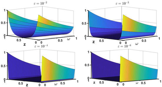
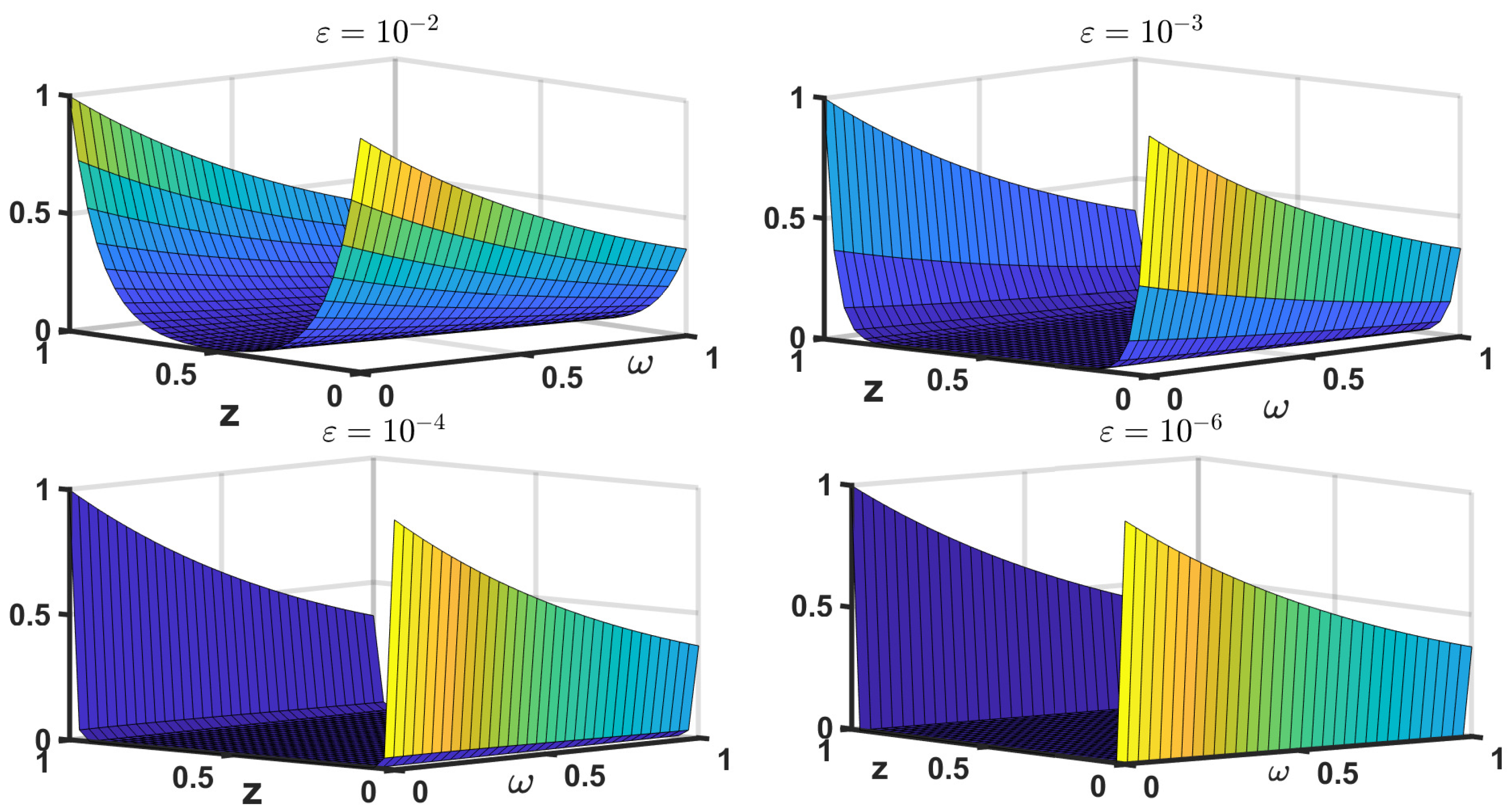
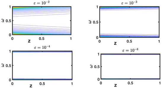
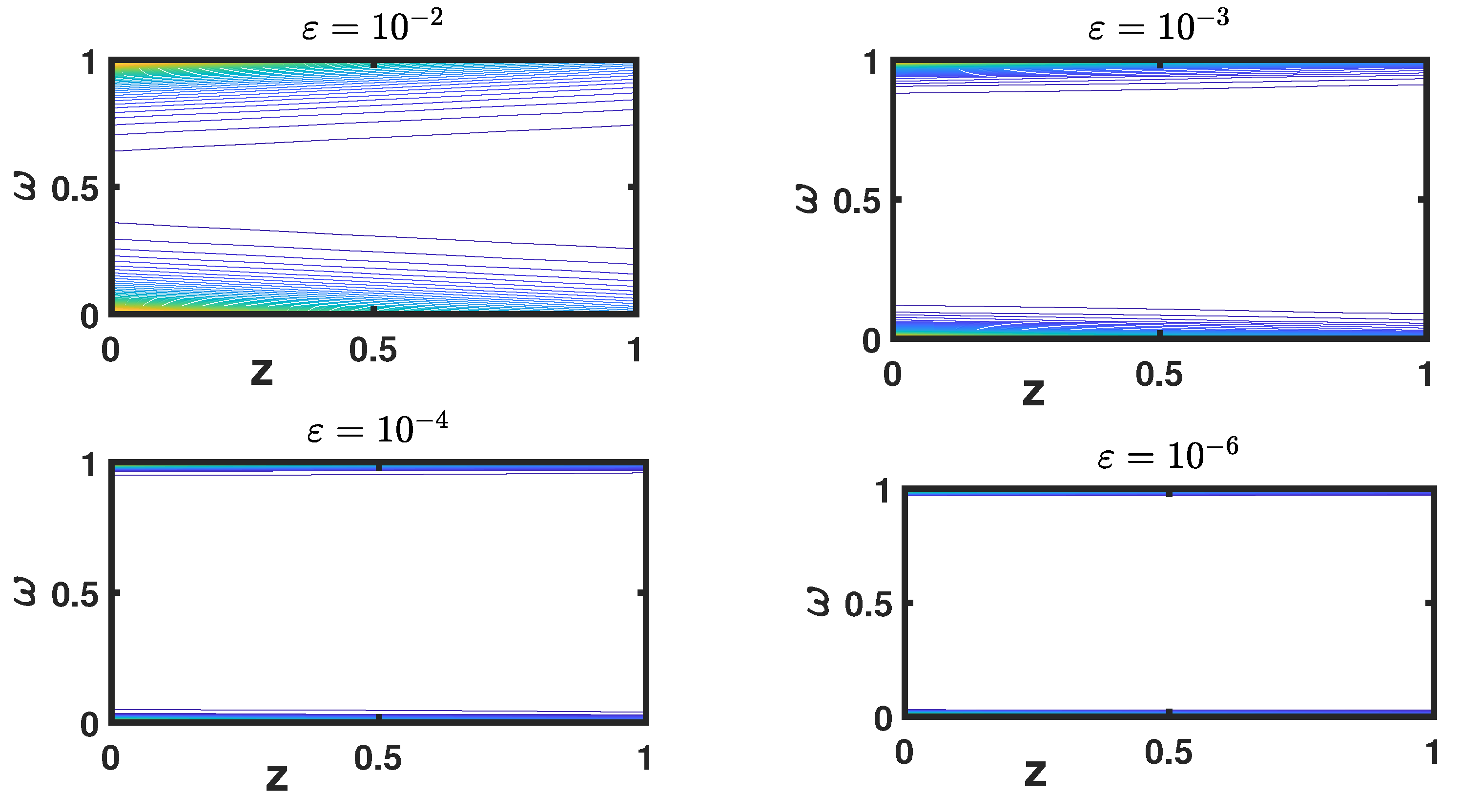
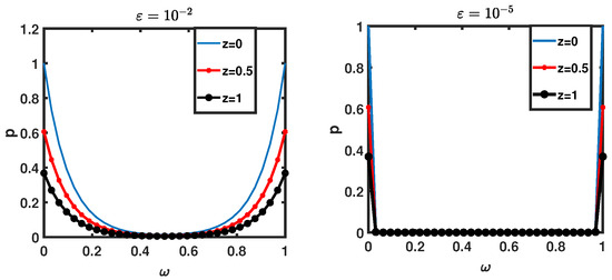
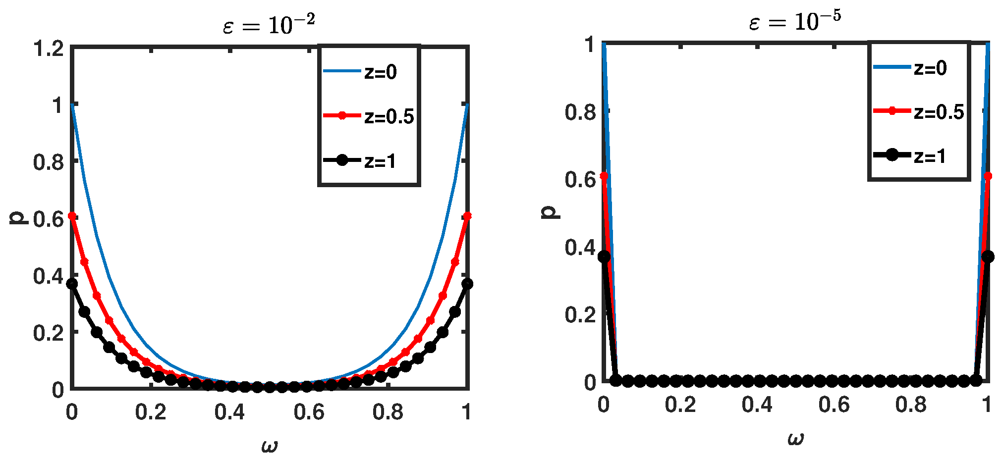
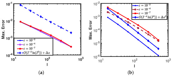
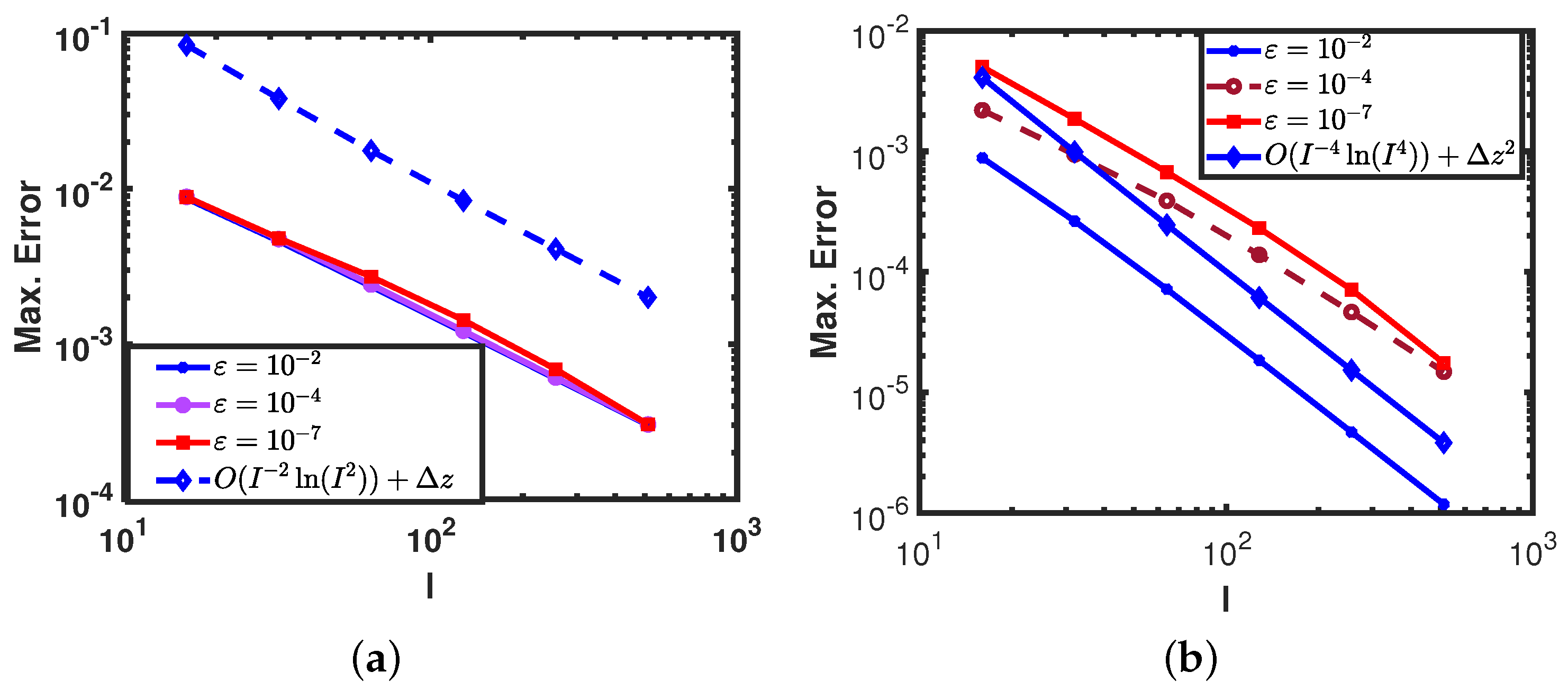
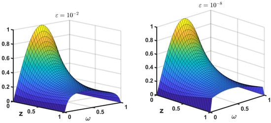
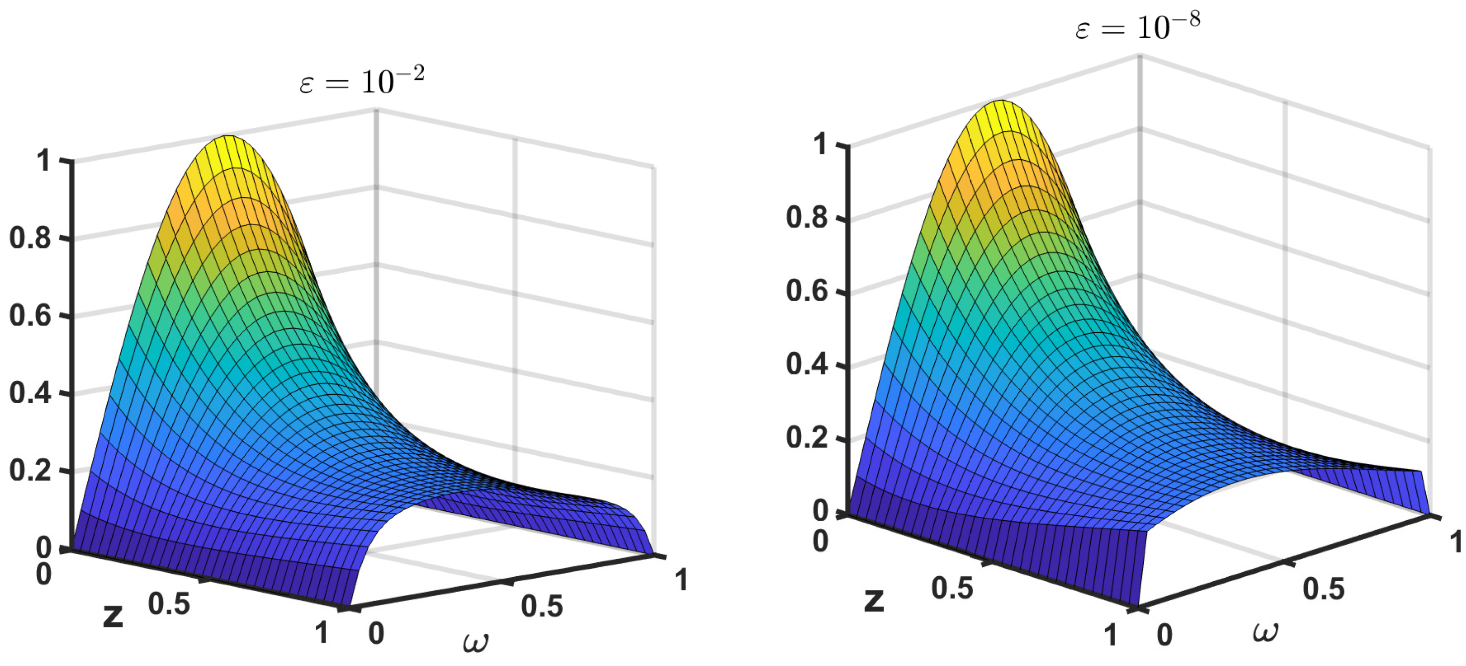
Figure 1 present the surface plots of the numerical solution for Example 10 and Example 11, while the corresponding contour plots are shown in Figure 2. Additionally, solution profiles at different time levels are displayed in Figure 3. These visualizations clearly illustrate the presence of boundary layers near and . The numerical order of convergence before and after extrapolation is illustrated in Figure 4, where the maximum pointwise errors are plotted on a log–log scale. Figure 5 present the surface plots of the numerical solution Example 11. Table 1 lists the values and before applying the RET for Example 10. The values given in Table 2 after RET of and the . In The data indicate that the time derivative term significantly influences the error. Notably, applying extrapolation nearly doubles the convergence rate, achieving second-order accuracy. To further improve accuracy, the time step is refined using . The results of this refinement are provided in Table 3, which demonstrates a clear trend toward fourth-order convergence. The results in Table 1, Table 2 and Table 3 generally confirm the expected uniform order of convergence. The few cases where the observed rate deviates (for example, when in Table 1) can be explained. For such extremely small perturbation parameters, the boundary layer becomes much narrower than the coarse mesh size, so the layer is not fully resolved at lower I. In addition, round-off effects become more noticeable when the solution is very steep. As the mesh is refined, the layer is captured correctly, and the rates quickly align with the theoretical order. These deviations are therefore a numerical artifact rather than a sign of instability of the method. In Table 4, we compare the execution time of the algorithm (in seconds) before and after extrapolation. It can be observed that the execution time increases after extrapolation, since a larger number of mesh intervals is required. However, this additional cost leads to improved accuracy.
Figure 1.
Surface plots of the numerical solution for Example 10.
Figure 2.
Contour plots of the numerical solution for Example 10.
Figure 3.
Solution plots of each time level for Example 10.
Figure 4.
Log-log plots of before and after extrapolation 10. (a) Before extrapolation. (b) After extrapolation.
Figure 5.
Surface plots of the numerical solution for Example 11.
Table 1.
Before applying extrapolation, the proposed method yields the following values for and .
Table 2.
After applying extrapolation, the proposed method yields the following values for and .
Table 3.
After applying extrapolation and step size reduce, the proposed method yields the following values for and .
Table 4.
Time comparison in seconds.
6. Conclusions
This paper presents a numerical approach for solving a parabolic integro-partial differential equation with small parameter of the form (1). The time derivative is discretized using the ‘implicit Euler method’ on a uniform mesh, while the spatial derivative is approximated using a central difference scheme on a ‘Shishkin mesh’, which ensures second-order accuracy in space. To enhance the convergence rate in both spatial and temporal dimensions, the RET is applied. We establish that the proposed method is uniformly convergent and achieves an approximate fourth-order accuracy. The effectiveness of the scheme is validated through numerical experiments on a benchmark problem. The results confirm that the method consistently achieves near-fourth-order convergence. The present study has focused on linear singularly perturbed problems with fixed- coefficient kernels. As part of future work, the proposed approach may be extended to more complex settings, such as nonlinear problems or variable-coefficient kernels. These generalizations are expected to pose additional analytical and computational challenges, but their successful treatment would considerably enhance the scope and applicability of the method to real-world models.
Author Contributions
Conceptualization, J.M.; Methodology, L.G., J.M. and T.A.N.; Software, L.G.; Validation, L.G., K.S.A.-G., J.M. and T.A.N.; Formal analysis, L.G. and J.M.; Resources, K.S.A.-G.; Data curation, K.S.A.-G. and T.A.N.; Writing—original draft, L.G. and J.M.; Writing—review & editing, T.A.N.; Supervision, J.M. All authors have read and agreed to the published version of the manuscript.
Funding
This research received no external funding.
Data Availability Statement
The original contributions presented in this study are included in the article. Further inquiries can be directed to the corresponding author.
Conflicts of Interest
The authors declare that they have no competing interests concerning the publication of the manuscript.
References
- Miller, J.J.H.; O’Riordan, E.; Shishkin, G.I. Fitted Numerical Methods for Singular Perturbation Problems; World Scientific: Singapore, 1996. [Google Scholar]
- Shishkin, G.I.; Shishkina, L.P. Difference Methods for Singular Perturbation Problems, 1st ed.; Chapman and Hall: Boca Raton, FL, USA, 2009. [Google Scholar]
- Abbaszadeh, M.; Dehghan, M. The interpolating element-free Galerkin method for solving Korteweg de Vries-Rosenau-regularized long-wave equation with error analysis. Nonlinear Dyn. 2019, 96, 1345–1365. [Google Scholar] [CrossRef] [Scilit]
- Ansari, A.R.; Bakr, S.A.; Shishkin, G.I. A parameter-robust finite difference method for singularly perturbed delay parabolic partial differential equations. J. Comput. Appl. Math. 2007, 205, 552–566. [Google Scholar] [CrossRef] [Scilit]
- Clavero, C.; Jorge, J.C.; Lisbona, F. A uniformly convergent scheme on a nonuniform mesh for convection-diffusion parabolic problems. J. Comput. Appl. Math. 2003, 154, 415–429. [Google Scholar] [CrossRef] [Scilit]
- Kamraniana, M.; Dehghan, M.; Tatari, M. An adaptive meshless local Petrov-Galerkin method based on a posteriori error estimation for the boundary layer problems. Appl. Numer. Math. 2017, 111, 181–196. [Google Scholar] [CrossRef] [Scilit]
- Rahman, M. Integral Equations and Their Applications; WIT Press: Southampton, UK, 2007. [Google Scholar]
- Kumar, M.; Sekhara Rao, S.C. High order parameter-robust numerical method for time, dependent singularly perturbed reaction-diffusion problems. Computing 2010, 90, 15–38. [Google Scholar] [CrossRef] [Scilit]
- Lange, C.G.; Smith, D.R. Singular perturbation analysis of integral equations. Stud. Appl. Math. 1993, 90, 1–74. [Google Scholar] [CrossRef] [Scilit]
- Sevgin, S. Numerical solution of a singularly perturbed Volterra integro-differential equation. Adv. Differ. Equ. 2014, 2014, 171. [Google Scholar] [CrossRef] [Scilit]
- Bala, S.; Govindarao, L.; Das, A.; Majumdar, A. Numerical scheme for partial differential equations involving small diffusion term with non-local boundary conditions. J. Appl. Math. Comput. 2023, 69, 4307–4331. [Google Scholar] [CrossRef] [Scilit]
- Elango, S.; Govindarao, L.; Awadalla, M.; Zaway, H. Efficient numerical methods for reaction–diffusion problems governed by singularly perturbed Fredholm integro-differential equations. Mathematics 2025, 13, 1511. [Google Scholar] [CrossRef] [Scilit]
- Sekar, E.; Govindarao, L.; Vadivel, R. A comparative study on numerical methods for Fredholm integro-differential equations of convection-diffusion problem with integral boundary conditions. Appl. Numer. Math. 2025, 207, 323–338. [Google Scholar]
- Linss, T.; Madden, N. Analysis of an alternating direction method applied to singularly perturbed reaction-diffusion problems. Int. J. Numer. Anal. Model. 2010, 7, 3507–3519. [Google Scholar]
- Amiraliyev, G.M.; Durmaz, M.E.; Kudu, M. A numerical method for a second order singularly perturbed Fredholm in-tegro-differential equation. Miskolc Math. Notes 2021, 22, 37–48. [Google Scholar] [CrossRef] [Scilit]
- Mukherjee, K. Parameter-uniform improved hybrid numerical scheme for singularly perturbed problems with interior layers. Math. Model. Anal. 2018, 2, 167–189. [Google Scholar] [CrossRef] [Scilit]
- Bansal, K.; Rai, P.; Sharma, K.K. Numerical treatment for the class of time dependent singularly perturbed parabolic problems with general shift arguments. Differ. Equ. Dyn. Syst. 2015, 25, 327–346. [Google Scholar] [CrossRef] [Scilit]
- Clavero, C.; Gracia, J.L.; Jorge, J.C. Higher order numerical methods for one-dimensional parabolic singularly perturbed problems with regular layers. Numer. Methods Part. Differ. Equ. 2005, 21, 149–169. [Google Scholar] [CrossRef] [Scilit]

Disclaimer/Publisher’s Note: The statements, opinions and data contained in all publications are solely those of the individual author(s) and contributor(s) and not of MDPI and/or the editor(s). MDPI and/or the editor(s) disclaim responsibility for any injury to people or property resulting from any ideas, methods, instructions or products referred to in the content. |
© 2025 by the authors. Licensee MDPI, Basel, Switzerland. This article is an open access article distributed under the terms and conditions of the Creative Commons Attribution (CC BY) license (https://creativecommons.org/licenses/by/4.0/).