Assessment of Simulated Meteorological Data Applicability for Hydrological Modelling in Low Land River Catchments

Abstract

Hydrological modelling in lowland catchments is often constrained by flat terrain and sparce meteorological station networks, which limits the accuracy of spatial interpolation of precipitation and temperature. In these conditions, the nearest available station may be located tens of kilometres away, making interpolated meteorological inputs highly uncertain and prone to systematic bias. This study aims to improve interpolated meteorological data for hydrological applications by developing and evaluating a practical bias correction approach suitable for low-relief regions with insufficient station density. Long-term temperatures and precipitation records from 18 meteorological stations in Lithuania (1961–2020) were used as reference data. Meteorological fields were reconstructed using Ordinary Kriging and Spline interpolation and evaluated against observations at monthly and daily time scales using correlation (r), Root Mean Square Error (RMSE), Percent Bias (PBIAS), Nash–Sutcliffe Efficiency (NSE), and Probability of Detection (POD) for precipitation. Bias correction was applied to interpolated datasets using inverse distance weighting (IDW) based on one to four neighbouring stations, reflecting typical distances of 50–70 km between observation sites. The results show that while the interpolation method strongly influences precipitation accuracy, bias correction substantially reduces systematic errors without altering temporal structure. The most robust improvements were obtained using two to three neighbouring stations and an IDW power parameter of one, particularly under flat terrain conditions. When applied as input to the HBV rainfall–runoff model for three representative lowland catchments, bias-corrected interpolated meteorological data consistently improved runoff simulations, bringing model performance closer to that achieved using historical station observations. The findings demonstrate that targeted bias correction is an effective and computationally simple strategy for improving interpolated meteorological data in data-sparse lowland regions. The proposed approach provides practical guidance for hydrological modelling where dense observation networks are unavailable and reliance on interpolation is unavoidable.

1. Introduction

Hydrological modelling in small lowland river catchments is often limited by incomplete, inconsistent, or spatially distant meteorological observations, particularly for precipitation and temperature [1,2]. In many regions, including Lithuania, the low station density and temporal gaps in long-term records reduce the reliability of model calibration and validation [3,4,5]. These limitations are especially critical in low-relief catchments, where subtle hydrological responses require high-resolution, and locally representative meteorological inputs to ensure robust modelling results [6].

The quality and origin of meteorological inputs strongly influence runoff simulations, as shown by global assessments of precipitation datasets. Beck et al. [3] evaluated 22 quasi-global precipitation datasets and found substantial differences in accuracy, with multi-source ensemble products such as Multi-Source Weighted-Ensemble Precipitation (MSWEP) generally performing best due to the integration of gauge, satellite, and reanalysis data. Sun et al. [5] reviewed 30 global precipitation datasets and reported deviations of up to 300 mm/year in annual precipitation estimates, highlighting the uncertainty associated with precipitation product selection. Recent global-scale hydrological evaluations confirm that the choice of precipitation dataset can significantly affect simulated discharge skill and bias [7]. Although conceptual models such as HBV can be forced with different meteorological inputs, their performance remains highly dependent on the consistency and representativeness of the input time series [4].

To supplement or replace incomplete station records, two main approaches are commonly used: spatial interpolation of historical observations and the use of reanalysis-based climate datasets [8,9]. Geostatistical interpolation methods, including Ordinary Kriging and Spline interpolation, have been widely used and often outperform simpler deterministic approaches by explicitly modelling spatial autocorrelation structures [10,11]. However, their performance remains strongly influenced by station density, data variability, and topographic complexity [8,11]. More advanced approaches, including kriging variants that incorporate auxiliary variables such as elevation or hybrid machine learning techniques, can further reduce prediction errors but still depend on the availability of representative training data [10,12,13]. Bias correction is frequently applied to meteorological datasets, particularly to regional and global climate model outputs [14,15], but it can also improve interpolated station-based data within small catchments. Inverse distance weighting (IDW) is widely used for spatial interpolation and bias transfer [16,17], and its application to correct interpolated meteorological inputs provides a practical means of reducing systematic errors before hydrological modelling.

Reanalysis datasets such as ERA5 offer a complementary alternative by providing globally consistent, physically constrained climate fields generated through data assimilation and numerical weather prediction [18]. Compared to ERA-Interim, ERA5 delivers higher spatial (~0.25°) and temporal (hourly) resolution, as well as improved agreement with independent observations [18]. Consequently, ERA5 has become increasingly popular for hydrological studies, particularly in regions with sparse in situ observations [19,20]. Although several studies report good overall performance of ERA5-driven hydrological simulations, notable regional differences persist, largely due to precipitation bias and spatial smoothing effects [19,20,21]. Bias correction techniques can enhance ERA5 suitability, but their effectiveness diminishes in data-poor regions where local observations for calibration are limited [22]. Despite these advancements, relatively few studies have systematically evaluated interpolated and reanalysis-derived meteorological data in lowland environments, where weak topographic gradients, sparse observation networks, and uneven station representativeness can amplify the hydrological impact of even small meteorological biases. In such settings, hydrological forcing is often dominated by a limited number of stations, and partial replacement of meteorological inputs (rather than full substitution) is a common but poorly quantified practice. The implications of this partial replacement for conceptual hydrological models such as HBV remain insufficiently documented.

This study addresses this gap by focusing on improving interpolated meteorological data for hydrological modelling in lowland environments characterised by flat terrain and sparse meteorological station networks. Rather than assessing the effects of substituting station observations with alternative data sources, the study treats spatial interpolation as a necessary condition in data-limited regions, where the nearest available station may be located tens of kilometres away. Using commonly applied interpolation techniques (Ordinary Kriging and Spline) and ERA5 reanalysis data as reference benchmarks, the analysis evaluates and enhances interpolated precipitation and temperature through bias correction. Drawing on long-term meteorological observations and three representative lowland catchments in Lithuania, the study systematically examines the effectiveness of inverse distance weighting (IDW)-based bias correction under conditions of insufficient station density. The HBV rainfall–runoff model serves as an independent validation framework to assess how improvements in meteorological bias affect hydrological performance. The results clarify the role of bias correction in reducing systematic errors in interpolated data and demonstrate practical correction configurations suitable for flat, data-sparse regions. The study thus provides application-oriented guidance for hydrological modelling where reliance on interpolated meteorological data is unavoidable.

2. Materials and Methods

2.1. Study Design and Workflow

This study was conducted in three sequential phases to evaluate the applicability of interpolated and reanalysis-based meteorological data for hydrological modelling in lowland river catchments. First, the accuracy of interpolated meteorological datasets (Ordinary Kriging and Spline) and ERA5 reanalysis data was assessed against observations from meteorological stations at both monthly and daily time scales. This step quantified the systematic bias and overall error characteristics of each dataset. Second, bias correction was applied to the interpolated meteorological datasets using inverse distance weighting (IDW) to identify robust correction configurations suitable for sparse station networks. The corrected datasets were evaluated using multiple statistical performance metrics, and a composite index was used to select the most effective correction scenarios for hydrological modelling. Finally, original, interpolated, bias-corrected, and ERA5-derived daily meteorological datasets were used as inputs to the HBV rainfall–runoff model to assess how uncertainty in meteorological forcing propagates into simulated river discharge. The resulting runoff simulations were compared with observed discharge to quantify the hydrological impact of alternative meteorological data sources.

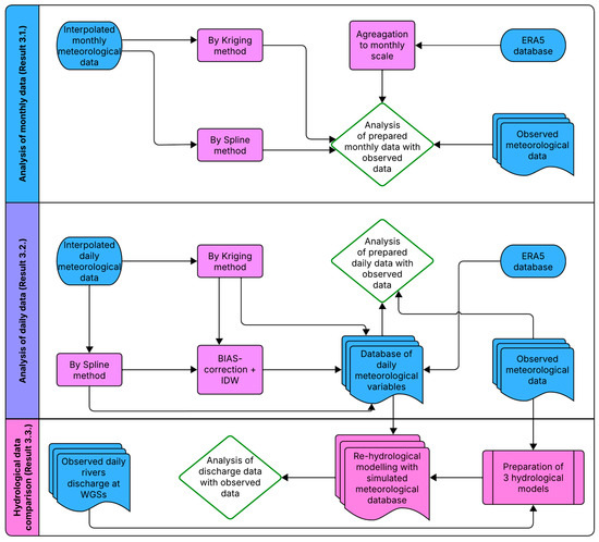
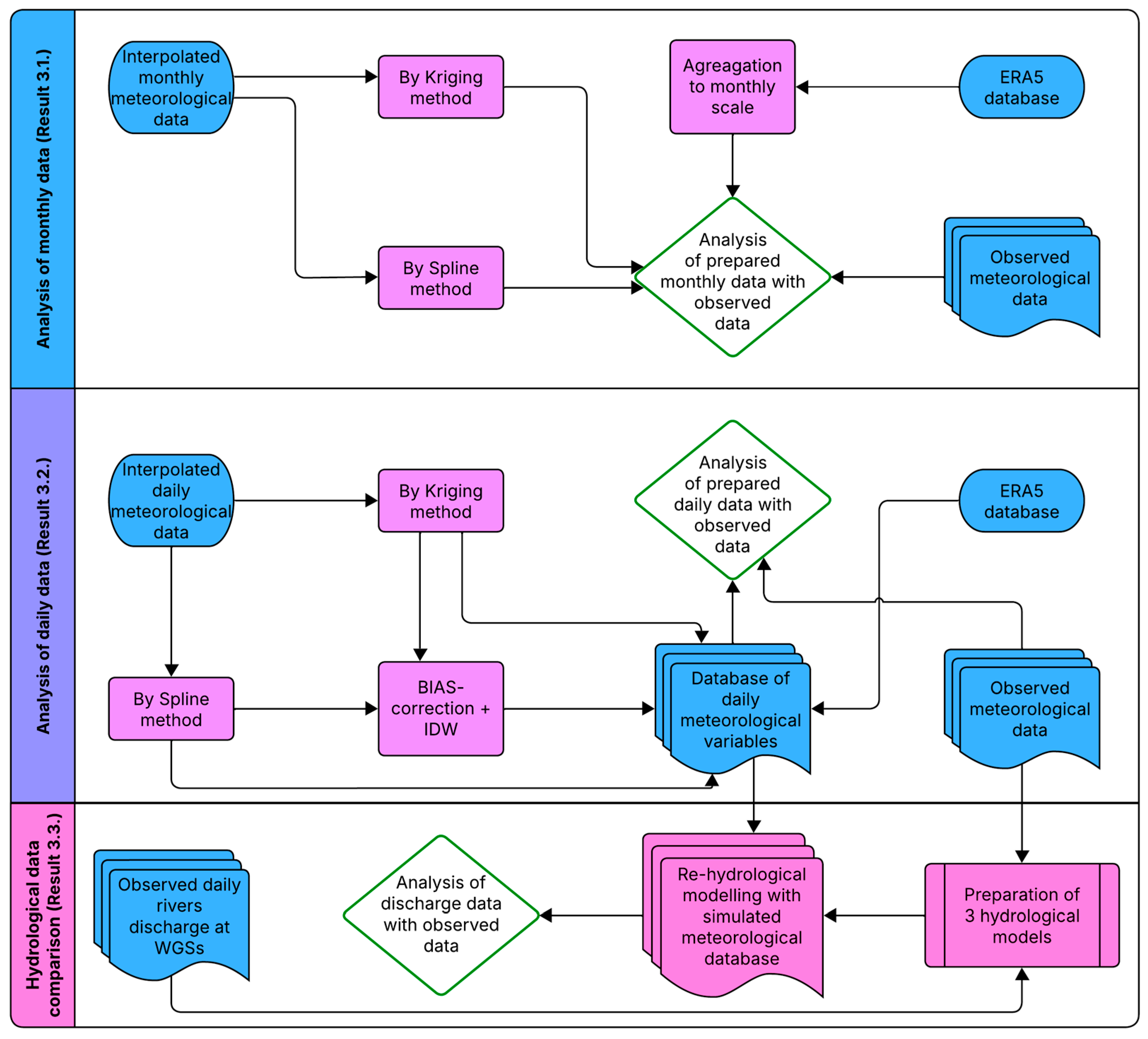
An overview of the methodological workflow and data flow between meteorological evaluation and hydrological modelling is presented in Figure 1.

Figure 1. Methodological framework illustrating the evaluation of interpolated and ERA5 meteorological data and their application in HBV hydrological modelling, including monthly and daily meteorological assessments, bias correction, and runoff simulation.

2.2. Meteorological Data and Study Area

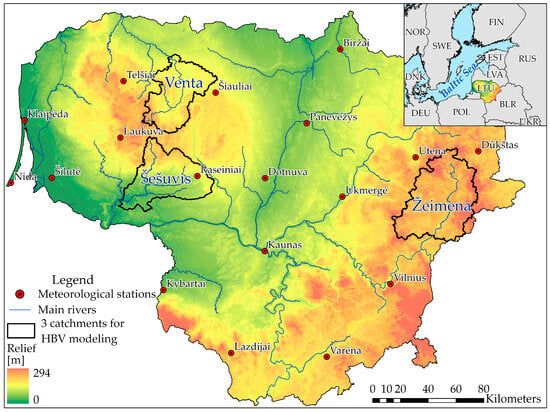
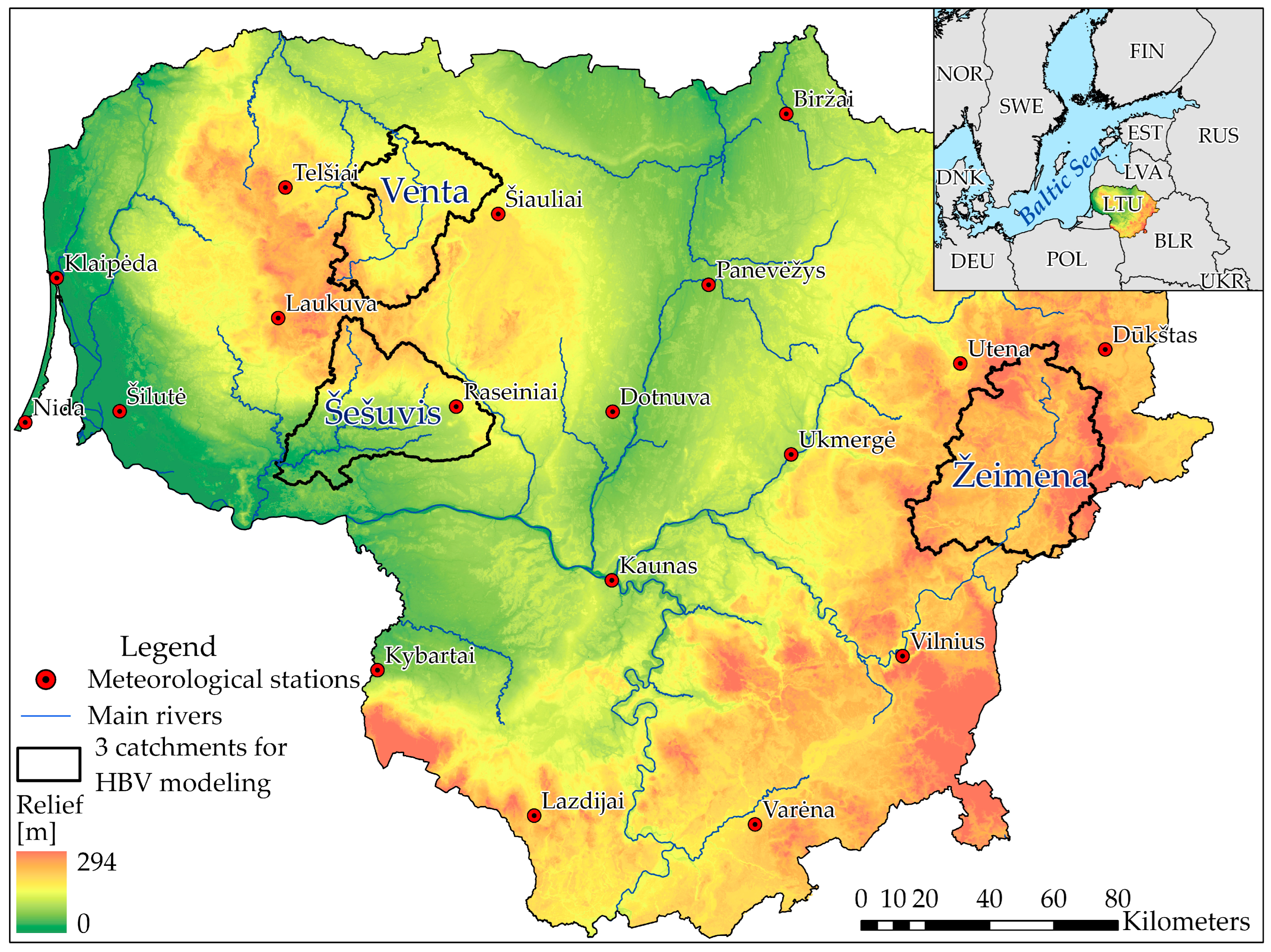
Meteorological data, including daily precipitation and air temperature, were obtained from 18 meteorological stations across Lithuania for the period 1961–2020 (Figure 2; Table 1). Four stations contained temporal gaps, while 14 stations provided continuous long-term records. These 14 stations were used as reference data for the monthly scale evaluation of interpolated and reanalysis-derived meteorological datasets.

Figure 2. Map of the study area indicating the distribution of meteorological stations, main river network, and the three lowland catchments (Venta, Šešuvis, Žeimena) used for HBV hydrological modelling.

Table 1. Meteorological stations (* stations which were used for daily analysis).

№	Station	Observation Period	Elevation [m]	P Average [mm/y]	T Average Winter [°C]	T Average Spring [°C]	T Average Summer [°C]	T Average Autumn [°C]
1.	Biržai	01.1961–12.2020	60	626.7	−3.70	6.07	16.7	6.80
2.	Dotnuva	01.1963–12.2020	69	571.2	−3.24	6.45	17.0	7.15
3.	Dūkštas *	09.1971–12.2020	164	615.3	−4.03	6.02	17.1	6.55
4.	Kaunas	01.1961–12.2020	76	633.0	−3.08	6.66	17.0	7.33
5.	Kybartai	01.1961–12.2020	58	599.1	−2.47	6.88	17.0	7.82
6.	Klaipėda	01.1961–12.2020	6	744.2	−1.02	6.00	16.6	8.94
7.	Laukuva *	01.1961–12.2020	165	797.3	−3.33	5.48	15.9	6.60
8.	Lazdijai	01.1961–02.1972, 01.1975–12.2020	133	608.0	−3.25	6.65	16.8	7.30
9.	Nida	01.1961–12.2020	2	728.3	−1.21	6.14	17.3	9.19
10.	Panevėžys	01.1961–12.2020	57	596.3	−3.35	6.37	16.9	7.05
11.	Raseiniai *	01.1961–12.2020	111	673.6	−3.41	5.98	16.2	6.87
12.	Šiauliai *	01.1961–12.2020	106	599.7	−3.20	6.01	16.7	7.09
13.	Šilutė	01.1961–12.2020	3	781.9	−1.97	6.52	16.7	7.98
14.	Telšiai *	01.1961–12.2020	153	783.6	−2.94	5.77	16.2	7.03
15.	Ukmergė	01.1961–12.2020	72	618.0	−3.44	6.48	16.9	7.19
16.	Utena *	01.1961–12.2020	105	658.7	−3.87	6.12	16.6	6.72
17.	Varėna	01.1961–12.2020	109	664.9	−3.50	6.39	16.8	6.95
18.	Vilnius *	04.1971–12.2020	162	677.0	−3.38	6.69	17.0	6.78

Seven stations with complete daily records for the period 1 January 1995 to 31 December 2014 were selected for daily scale analysis and hydrological modelling (Table 1). These stations represent the primary meteorological forcing for the three selected lowland catchments.

ERA5 reanalysis data were obtained via the Open-Meteo interface using the exact geographic coordinates of each meteorological station. ERA5 provides hourly meteorological fields at approximately 0.25° spatial resolution, which were aggregated to daily and monthly values to ensure temporal consistency with station observations.

All datasets underwent preprocessing, including quality control, temporal alignment, and extraction of comparable time series at station locations. Monthly data were used for preliminary evaluation of interpolation and reanalysis performance, while daily data were used for bias correction and hydrological modelling (https://open-meteo.com/).

2.3. Interpolation Methods

Two spatial interpolation techniques were applied to reconstruct temperature and precipitation fields across the study area: Ordinary Kriging and Spline interpolation.

Ordinary Kriging is a geostatistical method that estimates values at unsampled locations based on the spatial autocorrelation structure of observed data. Interpolation was performed using the 12 nearest meteorological stations for each predicted location.

Spline interpolation is a deterministic method that fits a smooth surface through input data points using piecewise polynomial functions.

Both methods were implemented in ArcGIS Pro 3.0.0. to generate daily and monthly raster surfaces at a 100 × 100 m spatial resolution. Interpolation was performed separately for each meteorological station, and interpolated values were extracted at station locations for accuracy evaluation. Negative precipitation values resulting from interpolation were set to zero.

2.4. Bias Correction and Interpolated Data

To improve the suitability of interpolated meteorological data for hydrological modelling, bias correction was performed using an inverse distance weighting (IDW) approach. The correction framework was designed for situations where data from the target station are unavailable and bias estimates must be transferred from neighbouring stations. Bias correction was performed using between one and four nearest stations, with spatial weighting controlled by the IDW power parameter p, ranging from 1 to 4.

For temperature, additive bias correction was applied, while precipitation correction used a multiplicative formulation. The corrected meteorological values were calculated using the following equations:

$${biasT}_{m,i}=\overline{T_{m,i}^{obs}}-\overline{T_{m,i}^{sim}},$$

(1)

where $T_{m,i}^{obs}$—observed temperature at station i for month m, $T_{m,i}^{sim}$—Interpolated temperature at station i, ${biasT}_{m,i}$—additive temperature bias at station i for month m.

$$w_i={\displaystyle \frac{d_i^{-p}}{{\sum }_{j=1}^N{d}_i^{-p}}},$$

(2)

where $w_i$—normalized IDW weight, $d_i$—distance from target point to station i, $p$—IDW power parameter, $N$—number of neighbouring stations.

$${biasT}_m^{target}=\sum _{i=1}^N{w}_i·{biasT}_{m,i},$$

(3)

where ${biasT}_m^{target}$—spatially transferred temperature bias at the target location.

$$T_m^{corr}\left(t\right)=T_{m,i}^{target}\left(t\right)+{biasT}_m^{target},$$

(4)

where $T_m^{corr}\left(t\right)$—BIAS-corrected temperature, $T_{m,i}^{target}\left(t\right)$—interpolated temperature at the target location.

Almost the same equations were used for precipitation, but instead the first and fourth equations were used for the next two, respectively:

$${biasP}_{m,i}={\displaystyle \frac{{\sum }_t{P}_{m,i}^{obs}\left(t\right)}{{\sum }_t{P}_{m,i}^{sim}\left(t\right)}},$$

(5)

where ${biasP}_{m,i}$—multiplicative precipitation bias factor, $P_{m,i}^{obs}\left(t\right)$—observed precipitation at station i, $P_{m,i}^{sim}\left(t\right)$—interpolated precipitation, $t$—time step.

$$P_m^{corr}\left(t\right)=P_{m,i}^{target}\left(t\right)·{biasP}_m^{target},$$

(6)

where $P_m^{corr}\left(t\right)$—BIAS-corrected precipitation, $P_{m,i}^{target}\left(t\right)$—interpolated precipitation at the target location, ${bias}_m^{target}P$—spatially transferred precipitation bias factor.

The performance of the corrected datasets was evaluated against observed data and compared with uncorrected interpolated datasets to assess improvements in bias, error magnitude, and overall consistency.

2.5. Reanalysis Data (ERA5)

ERA5 reanalysis data, produced by the European Centre for Medium-Range Weather Forecasts (ECMWF), were used as an alternative meteorological forcing dataset. ERA5 combines observations with numerical weather prediction through data assimilation, providing globally consistent climate fields at a high spatial resolution of approximately 0.25°.

For this study, daily ERA5 precipitation and temperature data were extracted at meteorological station locations using geographic coordinates. The data were aggregated to monthly values for preliminary evaluation and prepared in the same format as the station-based and interpolated datasets. No bias correction was applied to the ERA5 data, allowing direct assessment of the hydrological impact of uncorrected reanalysis forcing.

2.6. Evaluation Metrics

The accuracy of interpolated and ERA5-derived meteorological datasets was assessed by comparison with observed station records using several standard statistical metrics.

• The Pearson correlation coefficient (r) measures the strength of linear association between datasets.
• The Root Mean Squared Error (RMSE) quantifies the overall magnitude of error:

$$RMSE=\sqrt{{\displaystyle \frac{1}{N}}{\sum }_{i=1}^N{\left(X_i-Y_i\right)}^2,}$$

(7)

where $X_i$ and $Y_i$ represent values from the evaluated and referenced datasets, respectively, and $N$ is the length of the time series.

• The Percent Bias (PBIAS) measures systematic over- or underestimation

$$PBIAS=100·{\displaystyle \frac{{\sum }_{i=1}^n(P_i-O_i)}{{\sum }_{i=1}^n{O}_i}},$$

(8)

where $O_i$—observed value, $P_i$—simulated value, $n$—number of observations.

PBIAS measures the systematic tendency of a dataset to overestimate (positive values) or underestimate (negative values) observations [23].

• The Nash–Sutcliffe Efficiency (NSE) evaluates predictive skill relative to observed variability:

$$NSE=1-{\displaystyle \frac{\sum {(Q_{obs}-Q_{sim})}^2}{\sum {(Q_{obs}-\overline{Q_{obs}})}^2}},$$

(9)

where $Q_{obs}$—observed value, $Q_{sim}$—modelled value, $\overline{Q_{obs}}$—mean of observed values.

For precipitation, the Probability of Detection (POD) was additionally used to assess event detection capability:

$$POD={\displaystyle \frac{H}{H+M}},$$

(10)

where H denotes correctly detected precipitation events and M represents missed events.

A composite index (CI) was used to provide an integrated assessment of model performance by combining multiple evaluation metrics into a single normalized indicator.

$$CI={\sum }_{k=1}^K{w}_k·M_k^{norm}$$

(11)

where $M_k^{norm}$—normalised metric (r, NSE, RMSE, PBIAS, POD), $w_k$—metric weight, $K$—number of metrics.

2.7. Hydrological Modelling with HBV

Hydrological simulations were carried out using the HBV (Hydrologiska Byråns Vattenbalansavdelning) conceptual rainfall–runoff model [4]. HBV is a semi-distributed conceptual model that simulates catchment runoff using daily precipitation and temperature inputs. The model represents the main hydrological processes through a set of interconnected conceptual reservoirs, including snow accumulation and melting, soil moisture storage, groundwater storage, and runoff routing.

Snow processes are simulated using a degree-day approach; soil moisture regulates evapotranspiration and groundwater recharge; and runoff generation is represented by upper and lower groundwater reservoirs. Runoff routing is performed using a triangular weighting function. The model is based on the following water balance equation [24]:

$$P-E-Q={\displaystyle \frac{d}{dt}}\left[SP+SM+UZ+LZ+V\right],$$

(12)

where P is precipitation, E is evaporation, Q is discharge, SM is soil moisture, SP is snowpack, UZ is upper groundwater zone, LZ is lower groundwater zone, V is lake or dam volume. Three lowland river catchments in Lithuania—the Šešuvis (Skirgailiai), Žeimena (Pabradė), and Venta (Papilė)—were selected based on the availability of long-term hydrometeorological observations (Figure 2). HBV was calibrated using historical station-based meteorological data for 1995–2004 and independently validated for 2005–2014. Calibration aimed to achieve balanced performance across multiple evaluation metrics rather than optimising a single criterion.

Model performance was evaluated using the correlation coefficient (r), NSE, RMSE, and relative error (RE%), following established hydrological model evaluation guidelines. Calibration and validation results are summarised in Table 2. Across all catchments, the HBV models demonstrated stable and robust performance, confirming the suitability of the calibrated parameter sets for assessing the hydrological impact of alternative meteorological datasets.

Table 2. Performance of HBV models during calibration (1995–2004) and validation (2005–2014) for the Šešuvis River, Žeimena River, and Venta River catchments. Metrics shown include the correlation coefficient (r), Nash–Sutcliffe Efficiency (NSE), and relative error (RE%).

River-WGS	Calibration (1995–2004)			Validation (2005–2014)
	r	NSE	RE%	r	NSE	RE%
Sesuvis-Skirgailiai	0.886	0.786	2.16	0.845	0.714	−2.36
Zeimena-Pabrade	0.809	0.655	−2.34	0.816	0.667	3.56
Venta-Papile	0.884	0.781	−5.49	0.782	0.611	4.35

3. Results

3.1. Evaluation of Monthly and Daily Precipitation and Temperature

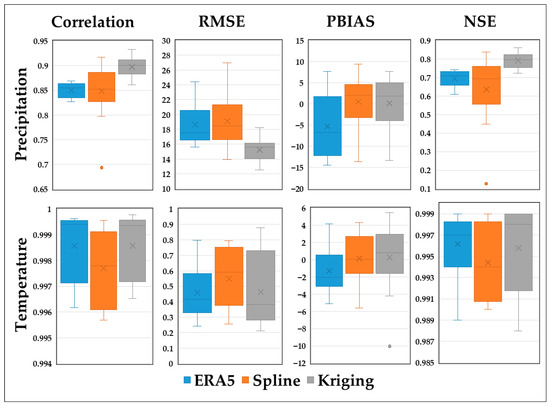
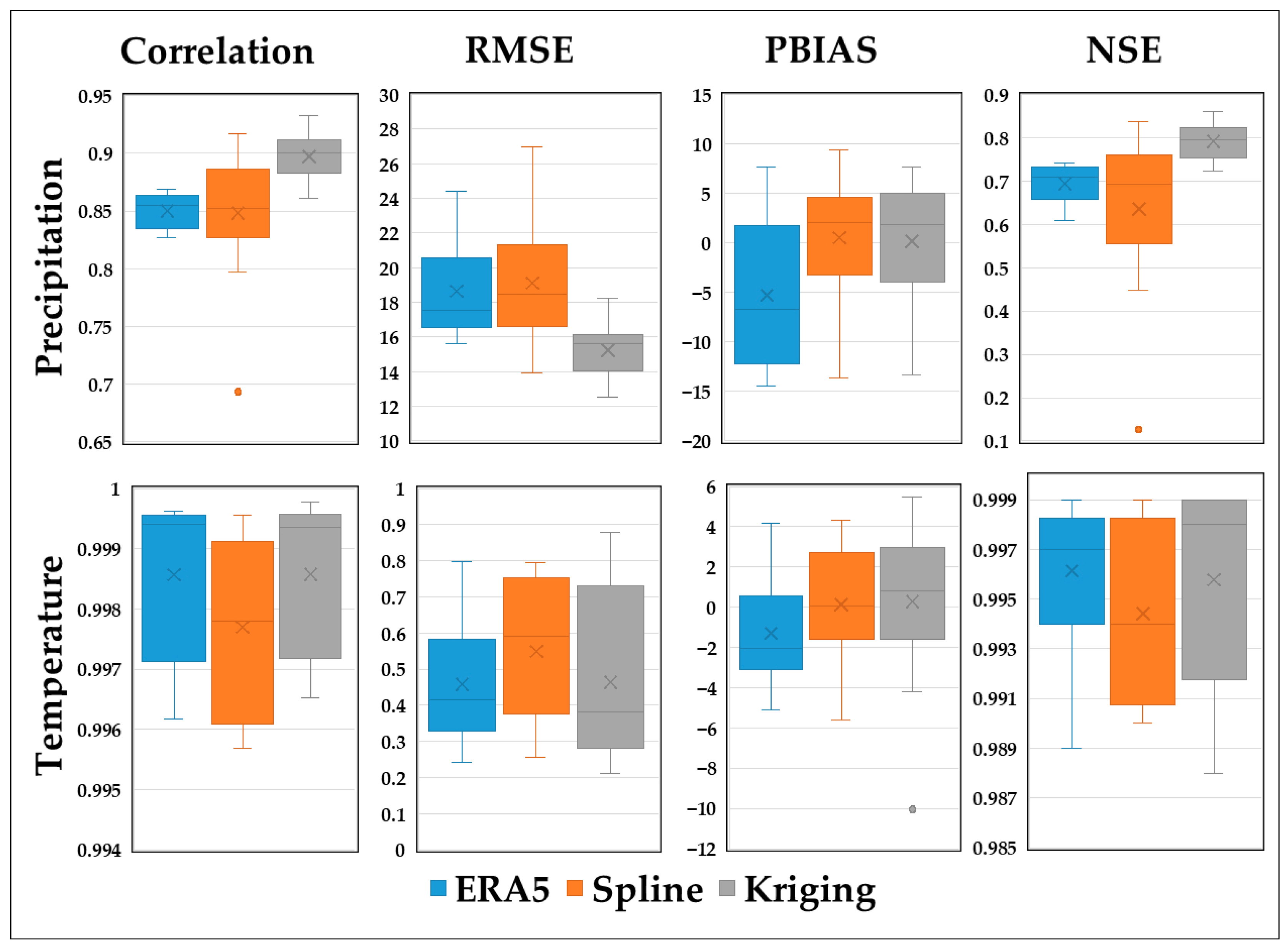
The performance of three precipitation data sources (ERA5 reanalysis, Spline interpolation, and Kriging) was evaluated at 14 meteorological stations (MS) in Lithuania (Figure 3) using four commonly used statistical indicators: Pearson correlation coefficient, Root Mean Square Error (RMSE), Percent Bias (PBIAS), and Nash–Sutcliffe Efficiency (NSE).

Figure 3. Statistical comparison of monthly precipitation and temperature datasets (ERA5, Spline, Kriging) with observations from 14 meteorological stations (MS).

During analysis of the monthly precipitation dataset, Kriging showed the highest correlation with observed station data, consistently reaching values above 0.90 at most sites, while spline interpolation yielded the lowest and most variable correlations, occasionally falling below 0.80 (Figure 3). For temperature, all three methods showed very strong correlations (above 0.99) with observed data across all stations, reflecting the inherently smoother and more stable nature of temperature fields. Across all stations, Kriging yielded the lowest RMSE values for monthly precipitation data, indicating the smallest deviations from the observed data. In contrast, Spline showed the highest RMSE in most cases, especially at the Biržai, Kybartai and Klaipėda stations (Figure 2). ERA5 showed an intermediate performance, although its errors remained considerable, especially at coastal stations such as Nida and Telšiai. All the stations listed are located on the edge (closer to the borders/outer stations), which may explain the high RMSE values for these stations. Despite high correlations in monthly temperature data across three datasets, Kriging provides the best RMSE performance in most cases. ERA5 errors tended to be slightly higher, especially in coastal areas such as Klaipėda and Nida, where the reanalysis data are more affected by maritime smoothing. The PBIAS metric showed ERA5 systematically underestimating monthly precipitation, with deviations often exceeding −10% at several stations. Kriging tended to produce more balanced or slightly negative deviations, whereas Spline often produced positive deviations, indicating a general overestimation. Also, Kriging achieved the most balanced PBIAS values (often close to zero) for the temperature dataset.

The NSE values, which quantify a model’s predictive ability, confirmed Kriging’s preference for the monthly precipitation dataset, with most stations achieving values above 0.75 and some exceeding 0.85 (Šilutė, Nida). ERA5 delivered relatively stable, though modest, NSE values for all stations. For monthly temperature, all methods produced extremely high NSE values, exceeding 0.99 in most cases, confirming excellent predictive ability (Figure 3). For all key performance metrics, Kriging interpolation of monthly meteorological data almost always shows better results compared to ERA5 and Spline. It achieved the highest correlation with ground truth data, the lowest RMSE, the smallest relative bias (PBIAS), and the highest predictive power (NSE). While ERA5 served as a useful baseline data source, it often showed overestimation and lower skill compared to interpolation methods. Spline interpolation, although widely used, showed inconsistent accuracy and greater sensitivity to station density and spatial configuration. ERA5 remains valuable in data-poor regions but requires local correction to reduce bias. The integration of Kriging with reanalysis data could be a promising approach to improving hydrometeorological inputs.

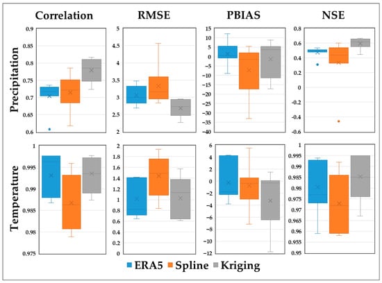
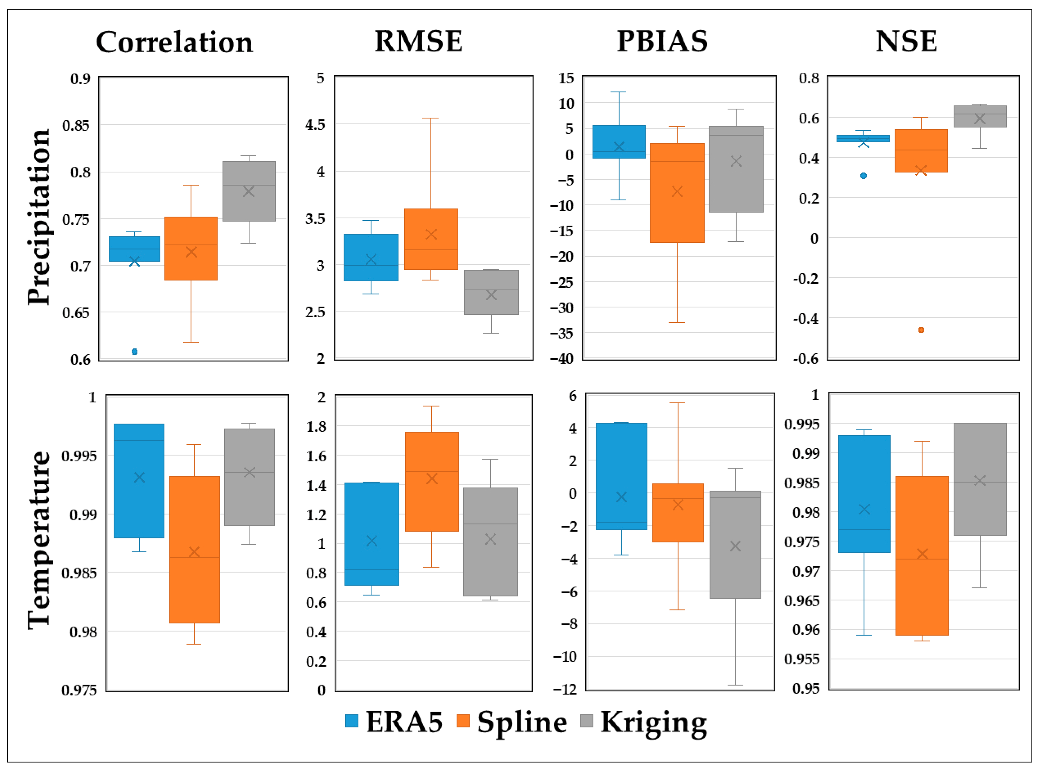
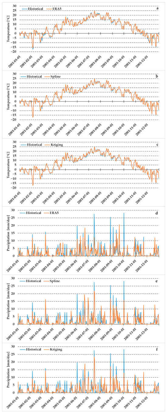
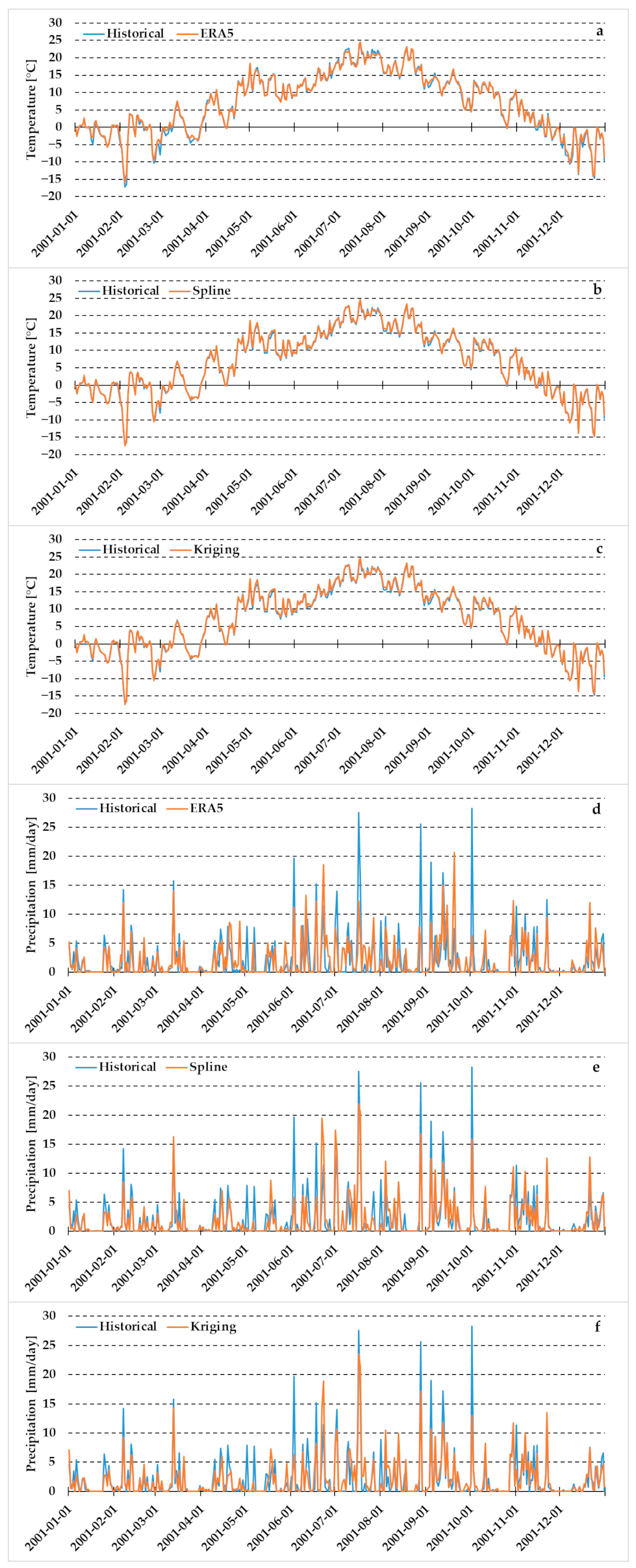
Daily temperature and precipitation datasets are very important for hydrological modelling. Therefore, data from seven meteorological stations were evaluated using ERA5, Ordinary Kriging, and Spline interpolation for the period 1995–2014. Figure 4 summarizes the statistical performance across all indicators, while Figure 5 provides an illustrative comparison of the daily time series for 2001 at the Raseiniai station.

Figure 4. Statistical comparison of precipitation and temperature daily datasets (ERA5, Spline, Kriging) with observations at seven meteorological stations in Lithuania for the period 1995–2014. Boxplots display the correlation coefficient (r), RMSE, PBIAS, and NSE values for each dataset.

Figure 5. Daily temperature and precipitation at the Raseiniai meteorological station in 2001, comparing historical observations with ERA5 (a,d), Spline (b,e), and Kriging (c,f) datasets.

The time-series plots (Figure 5) confirm that all datasets closely reproduce both the seasonal cycle and day-to-day temperature fluctuations, while precipitation datasets show larger deviations.

Across the stations, daily temperature showed very high correlations (>0.98) for all methods (Figure 4). Daily precipitation exhibited much greater differences among the datasets. Kriging achieved the highest correlations at six of the seven stations, with values generally between 0.70 and 0.80, indicating robust representation of spatial rainfall patterns. Spline produced the lowest and most variable correlations, with several stations near 0.60. This behavior reflects the high spatial heterogeneity of daily rainfall and the sensitivity of deterministic interpolation to station spacing.

RMSE patterns further highlighted the relative strengths of the methods. For daily temperatures, ERA5 and Kriging showed comparable RMSEs. Kriging produced the lowest RMSE of daily precipitation at most inland stations, whereas Spline showed the highest errors, particularly in areas influenced by local convective precipitation. Several consistent patterns according to Percent Bias (PBIAS) values showed no single dominant trend across stations. PBIAS values for daily temperature were small for all datasets (<±3%), but ERA5 showed the most balanced distribution, whereas Kriging displayed slightly negative deviations. For daily precipitation, ERA5 generally exhibited negative bias, systematically underestimating daily rainfall totals. Kriging produced PBIAS values closest to zero and with the lowest inter-station variability, while Spline displayed the widest range of biases, including substantial overestimation at inland stations and strong underestimation at peripheral sites such as Dūkštas (Figure 2). Nash–Sutcliffe Efficiency values were markedly lower for daily precipitation than for monthly data, reflecting the difficulty of accurately simulating high-frequency rainfall variability. Kriging produced the highest NSE values for nearly all stations (typically 0.55–0.70), demonstrating its excellent ability to reproduce daily precipitation dynamics. Spline frequently produced poor performance, including negative NSE values at Dūkštas, indicating a failure to represent daily rainfall processes in sparsely monitored regions. According to ERA5 data, the Dukstas MS has the best value, which is probably explained by the inclusion of other stations located outside Lithuania in the reanalysis.

Overall, the evaluation shows that daily precipitation is highly sensitive to the choice of meteorological dataset, whereas daily temperature is reliably reproduced by all methods. Kriging provides the best overall accuracy and stability for both variables, particularly for precipitation. ERA5 offers consistent performance and is especially valuable in data-scarce regions, though its systematic precipitation overestimation should be considered. Spline interpolation performs weakest at the daily scale, particularly for precipitation, and is strongly influenced by station density and proximity to the study area boundaries. These findings underscore the importance of selecting locally optimised datasets when preparing meteorological inputs for hydrological modelling in lowland basins.

3.2. Comparative Analysis of Meteorological Data with and Without BIAS Correction

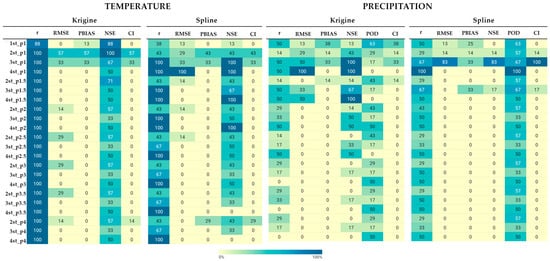
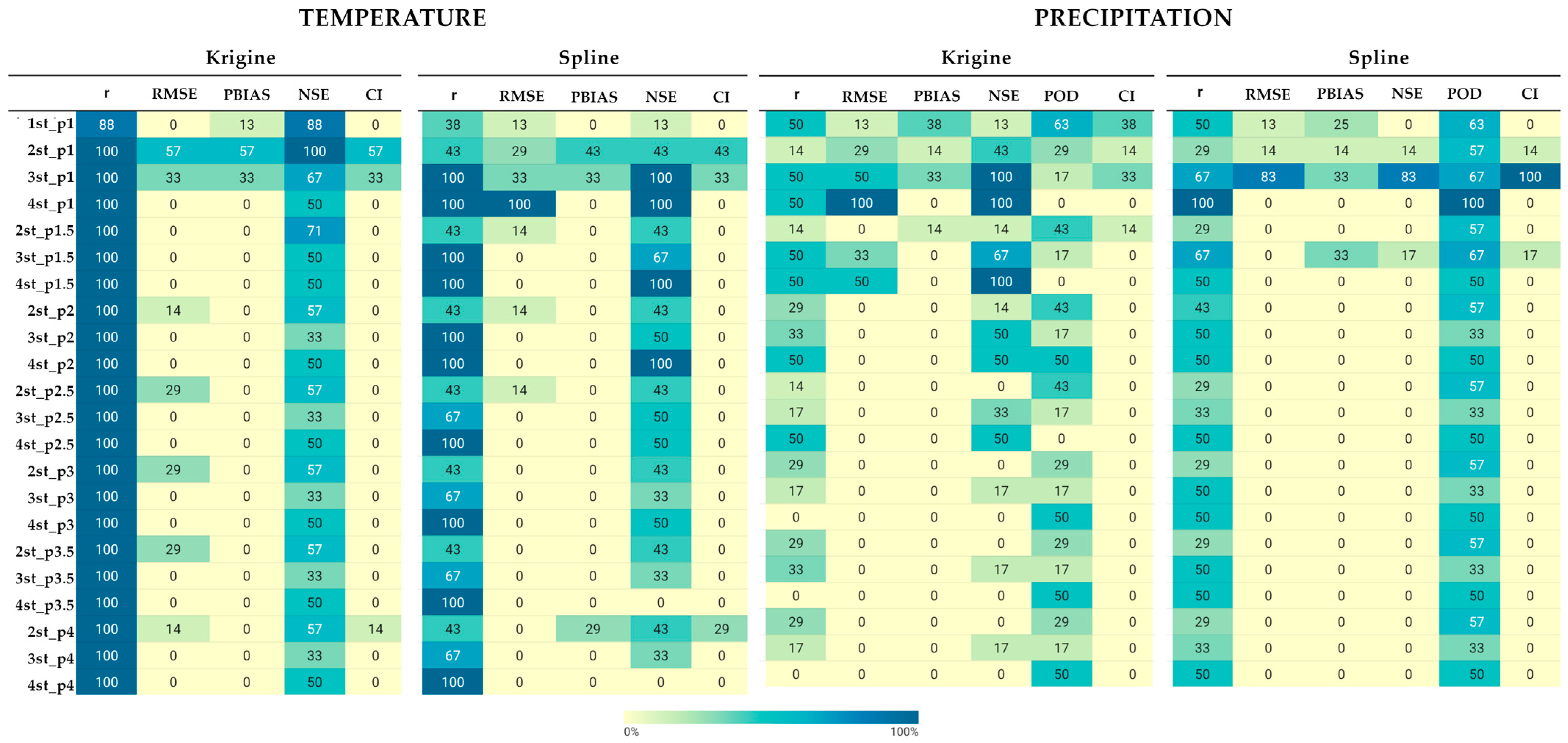
After BIAS correction of the interpolated meteorological data, numerous data sets were obtained in accordance with various input parameters. Figure 6 summarizes the performance of different bias correction scenarios applied to interpolated temperature and precipitation data using Kriging and Spline methods. Each scenario is defined by the number of neighbouring stations used for bias transfer (from 1 to 4) and the IDW power parameter p (from 1.0 to 4.0). For each scenario, the table reports the percentage of stations (out of seven) for which the given configuration produced the best performance according to individual evaluation metrics (r, RMSE, PBIAS, NSE, POD) and a composite index (CI). A value of 100% indicates that the scenario was best for all seven stations, whereas lower values indicate reduced robustness across the station network. More detailed values for each correction scenario are presented in Appendix A.

Figure 6. Frequency of optimal performance across seven stations for different bias correction scenarios defined by the number of neighbouring stations and IDW power parameter. Values represent the percentage of stations for which a given scenario yielded the best performance according to each metric.

According to the results shown in Figure 6 and Appendix A, it can be concluded that after BIAS correction, the correlation between new sets of meteorological data and historical data remains practically unchanged compared to data that was only interpolated. This applies to precipitation and temperature for both interpolation methods, and the deviations do not exceed 0.005. The RMSE and NSE values show slightly greater variability, but they are also insignificant compared to the interpolation values without correction. The POD values are also similar to the original data. The PBIAS values show significantly greater changes, with fluctuations reaching 11% for temperature and 23% for precipitation.

For temperature, the results indicate that bias correction based on Kriging and Spline using 2–3 stations with IDW power values (p) equal to 1 show the highest frequencies of optimal performance (Figure 6), suggesting that such methods of spatial averaging improve the stability of temperature bias correction better than others. There is also an advantage that for large distances between stations (50+ km), temperature correction using the 2 nearest stations is most effective.

For precipitation, the performance is more sensitive to the correction setup. While both Kriging and Spline approaches show high results, the outputs highlight a stronger dependence on the number of neighbouring stations and the IDW parameter p, especially for POD and NSE. In general, scenarios with two or three stations and p-values 1–1.5 exhibit higher robustness across the network (Figure 6).

3.3. Runoff Changes in Hydrological Models

This section describes research on how variability in meteorological data affects modeled river hydrological processes. Three hydrological models were developed for representative lowland catchments: Šešuvis River (catchment area to Skirgailiai WGS), Žeimena (area to Pabradė WGS), and Venta (area to Papilė WGS). At first, each model was calibrated and validated using historical station-based precipitation and temperature data. After achieving satisfactory model performance, the calibrated models were re-run using meteorological inputs generated from Kriging and Spline interpolation, BIAS-corrected interpolated data (the 5 best options for each model), and ERA5 reanalysis, allowing a direct assessment of the hydrological impacts arising from each data source.

Because hydrological models rely on areal averages of precipitation and temperature, the relative influence of each meteorological station within a catchment depends on its spatial contribution to the Thiessen-weighted precipitation and temperature inputs. For the hydrological model of the Šešuvis River, the meteorological stations of Raseiniai and Laukuva represented 61.2 and 38.8% of the catchment area, respectively; for the Žeimena River—Utena (40%), Dūkštas (36.2%) and Vilnius (23.8%); and for the Venta River—Telšiai (69.0%), Šiauliai (12.5%) and Laukuva (18.5%).

The following section presents the hydrological modelling results for each catchment and assesses how runoff simulations respond to alternative meteorological data obtained using Kriging and Spline methods with and without BIAS correction, as well as using ERA5 datasets.

3.3.1. Meteorological Data Impact on Runoff Modelling Results in the Šešuvis River

To model runoff in HBV, in addition to meteorological data obtained from ERA5, Kriging and Spline interpolation, the 5 best corrections of interpolated precipitation and temperature were selected, including one data set combining different correction methods, in accordance with the results shown in the previous section. The modelling results are shown in Table 3. The interpolated meteorological data without bias correction produces moderate performance (e.g., NSE = 0.644), while the application of IDW-based bias correction significantly improves the results. Among the tested configurations, Kriging-based bias correction using a combined method (in this case, it is 1–3 neighbouring stations and p-value 1.0) yields the highest performance, with NSE values reaching up to 0.727 and substantially reduced bias (PBIAS ≈ 10%). Such results are the best option for replacing meteorological data in the Šešuvis River catchment. Overall, bias correction for the Kriging method improved results and brought them closer to those modelled with real data.

Table 3. Evaluation of streamflow simulations using ERA5, interpolated and bias-corrected meteorological data for the Šešuvis River catchment. The bold values reflect the best results from the simulated.

Skirgailiai WGS—Observed Discharge
Variable		r	RMSE	PBIAS	NSE
Historical data		0.885	10.954	−0.513	0.758
ERA5		0.816	13.703	13.384	0.621
Kriging	Int	0.855	13.272	14.648	0.644
	2st_p1	0.869	12.241	9.209	0.698
	3st_p1	0.867	12.334	9.772	0.693
	4st_p1	0.868	12.259	9.155	0.697
	2st_p1.5	0.869	12.221	9.084	0.699
	Comb_bias	0.873	11.626	4.203	0.727
Spline	Int	0.864	12.920	10.936	0.663
	4st_p1	0.863	13.209	16.112	0.648
	3st_p1	0.862	13.360	17.230	0.640
	4st_p1.5	0.863	13.227	16.309	0.647
	3st_p1.5	0.862	13.333	17.087	0.641
	Comb_bias	0.862	13.243	16.365	0.646

The runoff obtained from interpolated data sets with bias correction did not show any significant positive change in this catchment area. ERA5 data have the worst metric values.

Overall, the results demonstrate that bias correction of Kriging interpolated meteorological data considerably enhances the quality of streamflow simulations for the Šešuvis River catchment, bringing model performance closer to that obtained using observed historical data.

3.3.2. Meteorological Data Impact on Runoff Modelling Results in the Žeimena River

The hydrological modelling results for the Žeimena River are presented in Table 4. This river runoff formation depends on meteorological data from three meteorological stations: Utena (40% from the catchment area), Dūkštas (36.2%) and Vilnius (23.8%). Interpolated meteorological data obtained by Kriging without error correction show good results compared to historical data but still exhibit a noticeable error for data interpolated by Spline (PBIAS = −22.03%). The application of IDW-based bias correction significantly improves model performance, especially for spline-based scenarios (Table 4). The results of spline-based scenarios increased by at least 16% in terms of PBIAS, and NSE increased from 0.253 to 0.640+. Kriging-based scenarios also perform better with bias correction and have the best results among all modelled data, which are almost identical to historical data, using 2 neighbouring stations with p = 1.0 or p = 1.5, achieving NSE values of up to 0.728 and significantly reducing bias (PBIAS between −0.7% and −1.0%). The use of ERA5 reanalysis data again gives results slightly lower than Kriging interpolation but higher than spline interpolation without correction.

Table 4. Evaluation of streamflow simulations using ERA5, interpolated and bias-corrected meteorological data for the Žeimena River catchment. The bold values reflect the best results from the simulated.

Pabradė WGS—Observed Discharge
Variable		r	RMSE	PBIAS	NSE
Historical data		0.852	4.533	−1.884	0.696
ERA5		0.826	4.925	−5.151	0.641
Kriging	Int	0.835	4.831	−6.523	0.655
	2st_p1	0.858	4.291	−0.727	0.728
	3st_p1	0.854	4.359	−1.577	0.719
	2st_p1.5	0.859	4.289	−0.955	0.728
	3st_p1.5	0.856	4.343	−1.765	0.721
	Comb_bias	0.854	4.332	−0.362	0.723
Spline	Int	0.806	7.111	−22.026	0.253
	2st_p1	0.836	4.774	−3.209	0.663
	2st_p1.5	0.837	4.760	−3.162	0.665
	3st_p1	0.833	4.937	−5.658	0.640
	3st_p1.5	0.836	4.888	−5.227	0.647
	Comb_bias	0.834	4.933	−5.588	0.640

Overall, the results demonstrate that bias correction of interpolated meteorological inputs considerably improves the quality of streamflow simulations at the Pabradė station, especially for Spline interpolation. Table 4 also shows that 2-station bias correction configurations provide the most robust results.

3.3.3. Meteorological Data Impact on Runoff Modelling Results in the Venta River

The Venta River runoff is influenced by precipitation and temperature from three meteorological stations (Telšiai MS covers 69% of the basin area, Šiauliai—12.5%, and Laukuva—18.5%). The use of interpolated meteorological data without bias correction shows a preference for the Spline method against Kriging interpolation for the Venta River catchment (NSE = 0.631 and PBIAS = 20.573% against NSE = 0.733 and PBIAS = −2.341% for Spline interpolation). Application of IDW-based bias correction leads to substantial improvements in model performance (Table 5). For Kriging-based scenarios, the best results are achieved with 3–4 neighbouring stations and p = 1.0–1.5, yielding NSE values of 0.715–0.731 and a considerable reduction in bias (PBIAS ≈ 3–9%).

Table 5. Evaluation of streamflow simulations using ERA5, interpolated and bias-corrected meteorological data for the Venta River catchment. The bold values reflect the best results from the simulated.

Papile WGS—Observed Discharge
Variable		r	RMSE	PBIAS	NSE
Historical data		0.843	6.562	0.776	0.711
ERA5		0.809	8.199	27.155	0.548
Kriging	Int	0.840	7.415	20.573	0.631
	4st_p1	0.858	6.513	9.034	0.715
	3st_p1	0.858	6.508	8.934	0.715
	4st_p1.5	0.858	6.461	7.824	0.719
	3st_p1.5	0.858	6.458	7.755	0.720
	Comb_bias	0.858	6.327	3.206	0.731
Spline	Int	0.858	6.301	−2.341	0.733
	3st_p1	0.868	6.089	−0.953	0.751
	4st_p1	0.868	6.093	−0.901	0.751
	3st_p1.5	0.868	6.081	−1.292	0.752
	4st_p1.5	0.868	6.081	−1.248	0.751
	Comb_bias	0.867	6.102	−0.760	0.750

The greatest improvements are observed for Spline-based bias correction, which provides the highest overall performance among all scenarios. Configurations using 3–4 neighbouring stations achieve NSE values up to 0.752, with near-zero bias (PBIAS between −1.3% and −0.9%) and lower RMSE values (≈6.08–6.10). ERA5 reanalysis data show the worst result compared to other meteorological datasets.

Overall, the results show that correcting interpolated meteorological data significantly improves runoff modelling at the Papile WGS, also in comparison with the two previous models Splines show the best results after BIAS correction, especially with a value of p 1.5. The comparison also shows that, unlike other stations, spline-based error correction slightly outperforms kriging-based approaches for this catchment.

4. Discussion

This study investigated the impact of different meteorological data sources and spatial bias correction strategies on streamflow simulations across three lowland river catchments. The results clearly demonstrate that the choice and preprocessing of meteorological inputs play a critical role in hydrological modelling performance, and that spatial bias correction substantially improves model reliability under data-scarce conditions.

Among the evaluated interpolation methods, Ordinary Kriging provided the most accurate reconstruction of meteorological variables, particularly precipitation, as indicated by higher correlation and lower RMSE and PBIAS values at both monthly and daily time scales. These results are consistent with previous studies demonstrating the robustness of geostatistical interpolation in climatological applications [10,11]. Spline interpolation showed the weakest statistical performance for precipitation, with lower correlations, higher RMSE, and pronounced positive biases. These findings are consistent with previous work [11]. The ERA5 reanalysis dataset demonstrated intermediate performance, positioned between Kriging and Spline. ERA5 consistently showed a negative precipitation bias, with PBIAS values often exceeding −10%. In monthly precipitation, ERA5 showed systematic positive bias, especially at coastal and peripheral stations. Similar bias patterns have been documented by several authors [18,19,20,21], who found that ERA5 data tend to overestimate weak and moderate precipitation and smooth out high-intensity events, especially in coastal, low-lying, and climatically complex regions.

The comparative analysis of meteorological data before and after bias correction showed that datasets remained largely unchanged after correction. In contrast, the most substantial improvements were observed for PBIAS, particularly for precipitation, where deviations of up to 23% were reduced after bias correction. This confirms that the main role of bias correction is to adjust the mean level of meteorological inputs. Similar findings have been reported in previous studies, showing that bias correction is especially effective at correcting systematic under- or overestimation of precipitation while preserving temporal patterns [25,26]. The results further indicate that bias correction based on two to three neighbouring stations and moderate IDW power values (p = 1.0–1.5) provides the most robust performance for both temperature and precipitation. This suggests that excessive spatial smoothing (large number of stations or high p-values) does not necessarily improve correction quality and may even reduce local representativeness, especially in low-land regions with sparse station networks (on average 50 km to the nearest station).

In all three catchment basins, river flow modelling based on meteorological data with corrected bias consistently outperformed modelling based on uncorrected interpolated data and reanalysis ERA5. This indicates the importance of data correction before using it in a hydrological model.

For the Šešuvis River, error correction based on the Kriging method yielded the most reliable results: NSE values increased from 0.644 (uncorrected interpolation) to 0.727, and PBIAS decreased from 14.6% to approximately 4%. In the Žeimena River catchment, error correction had an even stronger effect, especially for spline interpolation. Without correction, the spline-based input data resulted in very low performance (NSE = 0.253, PBIAS = −22%), whereas error correction increased NSE to over 0.64 and reduced error to less than −6%. Kriging-based error correction achieved the best overall performance, with NSE values up to 0.728 and an error close to zero. For the Venta River, the strongest improvements were obtained using spline-based bias correction. In this case, spline scenarios with bias correction slightly outperformed kriging-based corrections, achieving NSE values of up to 0.752 and PBIAS close to zero. These improvements brought the models’ performance closer to that obtained with historical observed data, confirming that spatial bias correction can effectively compensate for missing station data.

An important methodological result of this study is that error correction using 2–3 stations in conditions of low weather station density is sufficient to obtain meteorological data. This also reflects trends for flat regions with a limited number of meteorological stations, where increasing the number of stations beyond three can lead to excessive error, unlike regions with a dense network of observation stations and the ability to successfully perform IDW correction over long distances [16]. At the same time, interpolation data obtained by the Kriging method always gives better results after BIAS correction compared to the original. The results of spline data correction are also noteworthy and generally improve the original data, but this should be done with greater caution. Frequency-based evaluation showed that configurations using two or three neighbouring stations are the most reliable in the station network. This confirms the assumption that meteorological errors are spatially correlated and can be effectively transferred via distance-weighted averaging.

The results also demonstrate that moderate IDW power values (p ≈ 1.0–1.5) provide the best balance between local representativeness and spatial smoothing. This confirms the authors’ [16,27] opinion that the value of p is usually not equal to 2. Higher p values tend to overestimate the nearest station, while lower p values result in excessive spatial averaging, both of which can reduce the quality of the correction.

Despite the positive results, some limitations should be acknowledged. First of all, it is a labor-intensive and lengthy process. Second, the HBV model and the calibration parameters introduce additional uncertainty, so even the best correction method may yield mediocre results. Lastly, the correction schemes applied primarily address systematic mean bias and do not explicitly correct distributional properties such as variance or frequency of rainy days, which may be important for impact studies focused on extreme events. It should also be noted that a formal quantitative assessment of uncertainty is beyond the scope of this study and requires separate research. Overall, the results show that spatial correction of interpolated meteorological data bias is a highly effective and computationally efficient approach to improving hydrological modelling in lowland regions with insufficient data. This method allows hydrological models to achieve performance levels close to those obtained with observation station data, making it a valuable tool for operational modelling, climate impact assessment, and scenario analysis when complete meteorological observations are not available.

5. Conclusions

According to the results obtained in this study, the following statements are valid for lowland regions and sparce meteorological station density:

• Kriging gives more accurate results in meteorological data interpolation; accordingly, runoff computation in hydrological modelling becomes more stable.
• Two–three neighbouring stations and moderate IDW power values (p = 1.0–1.5) provide the most robust performance for both temperature and precipitation datasets for low-land areas and low meteorological station density.
• BIAS correction clearly outperforms approaches without corrections in the case of using such data for hydrological modelling.
• Kriging interpolation with Bias correction is more stable according to Spline-based datasets for hydrological modelling.
• Error correction using IDW with variable p can significantly improve the meteorological dataset.

References

- Brleković, T.; Tadić, L. Hydrological Drought Assessment in a Small Lowland Catchment in Croatia. Hydrology 2022, 9, 79. [Google Scholar] [CrossRef] [Scilit]
- Zhang, J.; Lian, Y.; Duan, Q.; Liu, Z.; Mao, X.; Ling, M.; Guan, Y. Coupled Hydrologic and Hydraulic Modeling for a Lowland River Basin in China. J. Hydrol. 2025, 649, 132470. [Google Scholar] [CrossRef] [Scilit]
- Beck, H.E.; Vergopolan, N.; Pan, M.; Levizzani, V.; van Dijk, A.I.J.M.; Weedon, G.P.; Brocca, L.; Pappenberger, F.; Huffman, G.J.; Wood, E.F. Global-scale evaluation of 22 precipitation datasets using gauge observations and hydrological modeling. Hydrol. Earth Syst. Sci. 2017, 21, 6201–6217. [Google Scholar] [CrossRef] [Scilit]
- Seibert, J.; Vis, M.J.P. Teaching hydrological modeling with a user-friendly catchment-runoff-model software package. Hydrol. Earth Syst. Sci. 2012, 16, 3315–3325. [Google Scholar] [CrossRef] [Scilit]
- Sun, Q.; Miao, C.; Duan, Q.; Ashouri, H.; Sorooshian, S.; Hsu, K.-L. A review of global precipitation data sets: Data sources, estimation, and intercomparisons. Rev. Geophys. 2017, 56, 79–107. [Google Scholar] [CrossRef] [Scilit]
- Wanzala, M.A.; Ficchi, A.; Cloke, H.L.; Stephens, E.M.; Badjana, H.M.; Lavers, D.A. Assessment of Global Reanalysis Precipitation for Hydrological Modelling in Data-Scarce Regions: A Case Study of Kenya. J. Hydrol. Reg. Stud. 2022, 41, 101105. [Google Scholar] [CrossRef] [Scilit]
- Gebrechorkos, S.H.; Leyland, J.; Dadson, S.J.; Cohen, S.; Slater, L.; Wortmann, M.; Ashworth, P.J.; Bennett, G.L.; Boothroyd, R.; Cloke, H.; et al. Global-scale evaluation of precipitation datasets for hydrological modelling. Hydrol. Earth Syst. Sci. 2024, 28, 3099–3118. [Google Scholar] [CrossRef] [Scilit]
- Hu, Q.; Li, Z.; Wang, L.; Huang, Y.; Wang, Y.; Li, L. Rainfall Spatial Estimations: A Review from Spatial Interpolation to Multi-Source Data Merging. Water 2019, 11, 579. [Google Scholar] [CrossRef] [Scilit]
- Longo, M.G.; Vanella, D.; Consoli, S.; Pappalardo, S.; Ramírez, C. Assessing the use of ERA5-Land reanalysis and spatial interpolation methods for retrieving precipitation estimates at basin scale. Atmos. Res. 2022, 271, 106131. [Google Scholar] [CrossRef] [Scilit]
- Goovaerts, P. Geostatistical Approaches for Incorporating Elevation into the Spatial Interpolation of Rainfall. J. Hydrol. 2000, 228, 113–129. [Google Scholar] [CrossRef] [Scilit]
- Li, J.; Heap, A.D. A review of comparative studies of spatial interpolation methods in environmental sciences: Performance and impact factors. Ecol. Inform. 2011, 6, 228–241. [Google Scholar] [CrossRef] [Scilit]
- Huang, J.; Lu, C.; Huang, D.; Qin, Y.; Xin, F.; Sheng, H. A Spatial Interpolation Method for Meteorological Data Based on a Hybrid Kriging and Machine Learning Approach. Int. J. Climatol. 2024, 44, 5371–5380. [Google Scholar] [CrossRef] [Scilit]
- Tobin, C.; Nicotina, L.; Parlange, M.B.; Berne, A.; Rinaldo, A. Improved interpolation of meteorological forcings for hydrologic applications in a Swiss Alpine region. J. Hydrol. 2011, 401, 77–89. [Google Scholar] [CrossRef] [Scilit]
- Kim, K.B.; Kwon, H.-H.; Han, D. Intercomparison of joint bias correction methods for precipitation and flow from a hydrological perspective. J. Hydrol. 2022, 604, 127261. [Google Scholar] [CrossRef] [Scilit]
- Skoulikaris, C.; Venetsanou, P.; Lazoglou, G.; Anagnostopoulou, C.; Voudouris, K. Spatio-Temporal Interpolation and Bias Correction Ordering Analysis for Hydrological Simulations: An Assessment on a Mountainous River Basin. Water 2022, 14, 660. [Google Scholar] [CrossRef] [Scilit]
- Chen, F.W.; Liu, C.W. Estimation of the spatial rainfall distribution using inverse distance weighting (IDW) in the middle of Taiwan. Paddy Water Environ. 2012, 10, 209–222. [Google Scholar] [CrossRef] [Scilit]
- Kurtzman, D.; Navon, S.; Morin, S. Improving interpolation of daily precipitation for hydrologic modelling: Spatial patterns of preferred interpolators. Hydrol. Process. 2009, 23, 3281–3291. [Google Scholar] [CrossRef] [Scilit]
- Hersbach, H.; Bell, B.; Berrisford, P.; Hirahara, S.; Horányi, A.; Muñoz-Sabater, J.; Nicolas, J.; Peubey, C.; Radu, R.; Schepers, D.; et al. The ERA5 Global Reanalysis. Q. J. R. Meteorol. Soc. 2020, 146, 1999–2049. [Google Scholar] [CrossRef] [Scilit]
- Tarek, M.; Brissette, F.P.; Arsenault, R. Evaluation of the ERA5 reanalysis as a potential reference dataset for hydrological modelling over North America. Hydrol. Earth Syst. Sci. 2020, 24, 2527–2544. [Google Scholar] [CrossRef] [Scilit]
- Gomis-Cebolla, J.; Rattayova, V.; Salazar-Galán, S.; Francés, F. Evaluation of ERA5 and ERA5-Land reanalysis precipitation datasets over Spain (1951–2020). Atmos. Res. 2023, 284, 106606. [Google Scholar] [CrossRef] [Scilit]
- Ferguglia, O.; Palazzi, E.; Arnone, E. Elevation dependent change in ERA5 precipitation and its extremes. Clim. Dyn. 2024, 62, 8137–8153. [Google Scholar] [CrossRef] [Scilit]
- Dhawan, P.; Torre, D.D.; Niazkar, M.; Kaffas, K.; Larcher, M.; Righetti, M.; Menapace, A. A comprehensive comparison of bias correction methods in climate model simulations: Application on ERA5-Land across different temporal resolutions. Heliyon 2024, 10, e40352. [Google Scholar] [CrossRef] [Scilit] [PubMed]
- Moriasi, D.N.; Arnold, J.G.; Van Liew, M.W.; Bingner, R.L.; Harmel, R.D.; Veith, T.L. Model Evaluation Guidelines for Systematic Quantification of Accuracy in Watershed Simulations. Trans. ASABE 2007, 50, 885–900. [Google Scholar] [CrossRef] [Scilit]
- SMHI. Integrated Hydrological Modelling System, Manual; Version 5.8; Swedish Meteorological and Hydrological Institute: Norrköping, Sweden, 2005. [Google Scholar]
- Gumindoga, W.; Rientjes, T.H.M.; Reggiani, P.; Makurira, H.; Haile, A.T. Hydrologic evaluation of bias corrected CMORPH rainfall estimates at the headwater catchment of the Zambezi River. Phys. Chem. Earth 2020, 115, 102809. [Google Scholar] [CrossRef] [Scilit]
- Probst, E.; Mauser, W. Evaluation of ERA5 and WFDE5 forcing data for hydrological modelling and the impact of bias correction with regional climatologies: A case study in the Danube River Basin. J. Hydrol. Reg. Stud. 2022, 40, 101023. [Google Scholar] [CrossRef] [Scilit]
- Noori, M.J.; Hassan, H.H.; Mustafa, Y.T. Spatial Estimation of Rainfall Distribution and Its Classification in Duhok Governorate Using GIS. J. Water Resour. Prot. 2014, 6, 75–82. [Google Scholar] [CrossRef]
Disclaimer/Publisher’s Note: The statements, opinions and data contained in all publications are solely those of the individual author(s) and contributor(s) and not of MDPI and/or the editor(s). MDPI and/or the editor(s) disclaim responsibility for any injury to people or property resulting from any ideas, methods, instructions or products referred to in the content. |
© 2026 by the authors. Licensee MDPI, Basel, Switzerland. This article is an open access article distributed under the terms and conditions of the Creative Commons Attribution (CC BY) license.