Multi-Objective Optimization of Surge Control Devices in Water Networks

Abstract

Hydraulic transients resulting from sudden pump shutdowns or valve closures can induce severe pressure fluctuations, known as water hammer, which compromise the safety and reliability of water distribution systems. Designing effective surge protection devices requires balancing hydraulic performance with economic feasibility, which naturally leads to a multi-objective optimization problem. This study develops an integrated framework that couples Don Wood’s Wave Plan Method for transient flow simulation with the Non-Dominated Sorting Genetic Algorithm II (NSGA-II) for optimal selection and design of water hammer arrestors. The proposed model simultaneously minimizes total installation cost and a hydraulic penalty function representing deviations in pressure from allowable limits. Decision variables include geometric and operational parameters of different surge protection devices such as air vessels, relief valves, and surge tanks, all constrained by practical hydraulic and physical limits. The resulting Pareto front illustrates the inherent trade-off between cost and reliability, enabling the identification of near-optimal design solutions. This approach provides a comprehensive basis for improving the hydraulic safety of pressurized water systems while maintaining economic efficiency, offering a flexible tool for future optimization and design studies in transient flow management.

1. Introduction

Hydraulic transients (water hammer) result from abrupt changes in flow conditions, such as valve closures or pump shutdowns, and can generate pressure surges that threaten the safety and reliability of pressurized water systems [1]. Since the foundational distributed-parameter model by Wood [2], transient flow modeling has advanced through wave-based and characteristic methods, with modern implementations available in tools such as TSNet [3,4,5,6]. When not adequately controlled, transients are commonly mitigated using devices such as air vessels, surge tanks, or relief valves, which are often designed using heuristic or single-objective approaches that overlook the trade-off between hydraulic protection and economic efficiency [7,8]. This trade-off naturally defines a multi-objective optimization problem.

Several multi-objective evolutionary algorithms have been proposed for engineering optimization problems, including SPEA-2, MOEA/D, NSGA-III, and multi-objective particle swarm optimization (MOPSO). Among these, NSGA-II is one of the most widely adopted due to its computational efficiency, fast non-dominated sorting, and effective diversity preservation using crowding distance [9,10]. Unlike weighted-sum or ε-constraint methods, NSGA-II does not require predefined objective weights and is well suited for capturing the full Pareto front in problems with conflicting objectives, with successful applications reported in hydraulic system optimization [10].

Despite these advances, most existing studies simplify cost formulations or focus on single surge protection devices, and few integrate detailed wave-based transient simulation with multi-objective optimization to jointly address hydraulic reliability and economic efficiency. The interaction between multiple protective elements within a unified optimization framework therefore remains insufficiently explored.

To address these gaps, the present study proposes an integrated framework that couples Don Wood’s Wave Plan Method for transient simulation with the NSGA-II algorithm for multi-objective optimization. The framework seeks the optimal type, configuration, and operational parameters of surge protection devices that minimize total installation cost while maximizing hydraulic reliability. A penalty-based performance index quantifies deviations in pressure heads from allowable limits, thereby linking the transient behavior of the system directly to the optimization objectives. Through successive evolutionary generations, the NSGA-II algorithm produces a Pareto front that reveals the trade-off between economic investment and surge mitigation effectiveness.

This study contributes to the growing field of intelligent hydraulic design by providing a unified methodology for analyzing and optimizing water hammer protection, where all surge protection devices are modeled and optimized simultaneously, allowing the transient solver to capture their coupled hydraulic response during pressure wave propagation.” The approach enhances the understanding of cost–reliability relationships in transient control and offers a decision-support tool for engineers designing safer and more efficient water distribution and transmission systems.

2. Literature Review

The study of water hammer, the rapid fluctuation in pressure resulting from sudden changes in fluid velocity, has been a central topic in hydraulic engineering for more than a century. Early analytical treatments were confined to simplified geometries and boundary conditions, but the advent of digital computation revolutionized transient flow analysis. A seminal contribution was made by Wood [2], who introduced a digital distributed-parameter model that numerically solved the governing continuity and momentum equations for unsteady flow in pipelines. This pioneering work established the computational foundation for modern transient analysis and provided the groundwork for the simulation tools used today.

Among the most influential numerical formulations that emerged from this foundation is the Method of Characteristics (MOC) [3]. The MOC transforms the governing partial differential equations into ordinary differential equations along characteristic lines, enabling the accurate propagation of pressure and velocity waves through both time and space. Owing to its physical transparency and numerical stability, the MOC has become the benchmark for transient flow analysis in both academic research and practical engineering applications. Nevertheless, when applied to large-scale systems or optimization-driven studies, the MOC can become computationally intensive because each simulation requires numerous time steps and iterative boundary updates. To overcome these computational challenges, Don J. Wood later developed the Wave Plan Method (WPM) [2], an efficient time-domain algorithm that models wave reflections and transmissions without the full characteristic-line integration required by the MOC. The WPM preserves the physical interpretation of wave propagation while simplifying numerical implementation, making it particularly suitable for iterative or optimization-based applications. Subsequent developments in transient modeling further expanded its capabilities, incorporating phenomena such as viscoelastic pipe-wall behavior [3], vapor cavity collapse [4], and wave-tracking algorithms [1], which enhance both numerical stability and predictive accuracy under severe transient conditions.

In recent years, the field has also benefited from the introduction of open-source computational frameworks. The TSNet package [5,6] provides a flexible Python-based environment for transient flow simulation in water distribution networks. This framework facilitates integration with optimization and control algorithms, encouraging reproducibility and collaboration across research institutions. The shift toward open and extensible modeling environments has accelerated innovation in transient analysis and network optimization.

Parallel to advances in transient modeling, significant progress has been made in surge protection and transient control. In engineering practice, devices such as air vessels, surge tanks, and pressure relief valves are commonly employed to mitigate pressure surges. Each device operates according to distinct principles: air vessels and closed surge tanks absorb excess energy through the compressibility of trapped air, while relief valves dissipate energy by releasing flow when system pressure exceeds a specified threshold. Early design methodologies for these devices were based primarily on empirical correlations or single-objective optimization criteria focused on minimizing peak pressure. Although practical, these approaches often overlooked the essential trade-off between hydraulic safety and economic feasibility. To address this limitation, researchers began incorporating optimization algorithms into transient protection design, using the impulse response [10] method in conjunction with a Genetic Algorithm (GA) to optimize surge tank dimensions for pressure attenuation. This approach was extended [10] to pump–reservoir systems, optimizing surge tank volume and throttle characteristics to reduce pressure extremes. These studies demonstrated the capacity of evolutionary algorithms to handle nonlinear, multi-parameter relationships inherent in surge protection problems. Building on these efforts, Lyu et al. [7] developed a combined protection strategy that optimized air vessel volume while considering both system performance and economic cost under multiple transient scenarios. Moreover, Zeidan and Ostfeld [8] explored the use of transient pressures for pipeline maintenance, illustrating the expanding applications of transient analysis beyond protective measures alone. Despite these advancements, most previous studies have employed single-objective formulations, targeting either hydraulic performance or cost minimization rather than addressing both simultaneously. In real-world engineering, enhancing system reliability typically demands larger or more responsive protective devices, which inevitably increases capital and maintenance expenditures. This inherent conflict defines a multi-objective optimization (MOO) problem that requires specialized algorithms to balance competing objectives.

The Non-Dominated Sorting Genetic Algorithm II (NSGA-II) [9] has emerged as one of the most effective tools for addressing such problems. NSGA-II employs an elitist selection mechanism and a crowding-distance metric to maintain diversity among non-dominated solutions, enabling it to approximate a well-distributed Pareto front that captures the full spectrum of trade-offs between objectives. The algorithm has been successfully applied in diverse fields, from financial portfolio management [9,11] to hydraulic and water system design [4,10]. When coupled with a transient solver such as the WPM or MOC, NSGA-II allows engineers to evaluate and optimize potential configurations of surge protection devices in terms of both hydraulic reliability and economic efficiency, ultimately yielding a set of Pareto-optimal design alternatives.

Nevertheless, important challenges remain. Many existing studies simplify cost formulations, restrict optimization to a single type of protective device, or disregard the influence of device location and network topology. These limitations highlight the need for a comprehensive framework that integrates Don Wood’s Wave Plan Method with NSGA-II to optimize the selection, configuration, and sizing of multiple surge protection devices simultaneously. Such an integrated approach enables realistic assessment of cost–reliability relationships and provides a robust, data-driven foundation for designing safer and more efficient water distribution and transmission systems under transient conditions.

3. Methodology

This study combines a detailed transient flow simulation using the WPM [2] with a multi-objective optimization framework based on the Non-Dominated Sorting Genetic Algorithm II (NSGA-II) [9]. The goal is to identify the optimal configuration and placement of surge protection devices that minimize system cost while maximizing hydraulic reliability.

3.1. Wave Plan Method

The WPM [2] is a numerical technique used to simulate and analyze hydraulic transients in pressurized pipe systems. The method was originally developed by Wood et al. [2] at the NASA Lewis Research Center to represent unsteady flow conditions in liquid-filled conduits. It is based on the concept of pressure wave propagation, which describes how rapid changes in velocity or boundary conditions generate pressure surges that travel along the pipeline at the wave speed of the fluid. In typical water systems, these pressure waves move at velocities ranging from 400 m/s in polymeric pipes to approximately 1000 m/s in metallic pipes, depending on the pipe material and wall elasticity [8]. Each wave carries information about changes in pressure and flow, and when it encounters a discontinuity—such as a valve, junction, reservoir, or change in pipe diameter—it is partially reflected and partially transmitted. The superposition of all these reflected and transmitted waves defines the complete transient response of the system.

The WPM discretizes the pipeline into a series of short segments and tracks the propagation of waves at discrete time intervals. Each incremental disturbance in discharge or head is considered as an independent “wave plan,” traveling a distance $\mathrm{\Delta }x=\alpha \mathrm{\Delta }t$ during the time step $\mathrm{\Delta }t$. The total head and discharge at any node and time are obtained by summing the effects of all incident waves reaching that point.

The relationship between the change in pressure head ($\mathrm{\Delta }H$) and the change in velocity ($\mathrm{\Delta }V$) is given by Equation (1), also known as the Joukowsky equation:

$$\mathrm{\Delta }H={\displaystyle \frac{\alpha \mathrm{\Delta }V}{g}}$$

(1)

where $a$ is the wave speed, and $g$ is the gravitational acceleration. This fundamental equation forms the basis of the WPM, linking the hydraulic response directly to the velocity disturbance that initiated it.

The wave speed $a$ is defined as follows:

$$\begin{array}{cccc}& a=\sqrt{{\displaystyle \frac{K}{\rho (1+\frac{DK}{Ee})}}}& & \end{array}$$

(2)

where $K$ is the bulk modulus of water, $\rho$ is the fluid density, $E$ is the Young’s modulus of the pipe wall, $D$ is the pipe diameter, and $e$ is the wall thickness. This expression accounts for both the elastic deformation of the pipe wall and the compressibility of water, which together determine the rate at which pressure information travels through the conduit.

At each computational step, the method determines the head and discharge at every node by considering the incoming and outgoing waves from adjacent segments. Reflections and transmissions at boundaries are calculated according to the impedance of each element, allowing the method to handle multiple branches, reservoirs, valves, and surge devices within a unified framework.

At each time step, the propagation distance of a wave is defined as follows:

$$\mathrm{\Delta }x=a\mathrm{\Delta }t$$

(3)

where $\mathrm{\Delta }x$ is the segment length and $\mathrm{\Delta }t$ is the computation time step.

This relation ensures numerical stability and physical consistency between spatial and temporal discretization.

The total hydraulic state at each node is determined from the combination of forward and backward traveling waves, expressed as characteristic variables:

$$\begin{array}{cccc}& H^{+}=H+{\displaystyle \frac{Q}{C}},\hspace{1em}\hspace{1em}{H}^{-}=H-{\displaystyle \frac{Q}{C}}& & \end{array}$$

(4)

where $C={\displaystyle \frac{a}{gA}}$ is the characteristic constant, $H$ is the piezometric head (m), and $Q$ is the discharge (m³/s).

At the end of each time step, the new head and discharge are obtained by superposition of the incoming waves from the two adjacent sections:

$$H_j^{t+\mathrm{\Delta }t}={\displaystyle \frac{H_{j-1\to j}^{+}+H_{j+1\to j}^{-}}{2}},\hspace{1em}\hspace{1em}{Q}_j^{t+\mathrm{\Delta }t}={\displaystyle \frac{C}{2}}(H_{j-1\to j}^{+}-H_{j+1\to j}^{-})$$

(5)

This formulation allows for an explicit, time-marching solution without requiring global matrix inversion, which makes the Wave Plan Method both efficient and robust for transient flow modeling [4].

When a wave encounters a discontinuity—such as a change in diameter, a junction, or a surge protection device—it is partially reflected and transmitted. The magnitude of reflection $R$ and transmission $T$ coefficients depends on the impedance ratio between adjacent sections:

$$\begin{array}{cccc}& R={\displaystyle \frac{Z_2-Z_1}{Z_2+Z_1}},\hspace{1em}\hspace{1em}T={\displaystyle \frac{2Z_2}{Z_1+Z_2}}& & \end{array}$$

(6)

where $Z={\displaystyle \frac{gA}{a}}$ is the hydraulic impedance.

This enables the WPM to simulate complex topologies and boundary interactions within a unified wave-based framework.

3.2. Device Modeling

Surge protection devices play a crucial role in controlling the magnitude and duration of hydraulic transients by either absorbing, storing, or dissipating excess hydraulic energy, and they are modeled as localized hydraulic boundary conditions with parameter-dependent pressure–discharge relationships, allowing their dynamic interaction with pressure wave propagation to be explicitly captured.

In the present work, three primary protection types are represented—relief valves, air vessels, and surge tanks—each formulated through distinct boundary condition equations within the WPM framework.

3.2.1. Relief Valve

A pressure relief valve provides rapid protection against overpressures by automatically opening when the local piezometric head $H_p$ exceeds a predefined set head $H_{\mathrm{set}}$. When activated, it releases water to the atmosphere, thereby converting hydraulic energy into kinetic energy and reducing the magnitude of reflected waves. The governing discharge relation is expressed as follows:

$$\begin{array}{cccc}& Q_v=\left\{\begin{array}{cc}\hfill C_d{A}_v\sqrt{2g(H_p-H_{\mathrm{set}})}, & H_p>H_{\mathrm{set}}\\ \hfill 0, & H_p\le H_{\mathrm{set}}\end{array}\right.& & \end{array}$$

(7)

where $C_d$ is the discharge coefficient and $A_v$ the valve orifice area.

This nonlinear boundary is solved iteratively within the WPM time-marching scheme.

The optimal relief valve calibration can limit surge peaks by 40–60% in pumping systems [10,11]. Combining air-inlet valves with relief valves yields superior damping during both over- and under-pressure phases. In large pumping mains, it was confirmed through KY PIPE simulations that relief valves are particularly effective when positioned near pumps or control valves, acting as the first line of defense against abrupt stoppages [4].

3.2.2. Air Vessel

An air vessel functions as an elastic energy reservoir that counters both over- and under-pressure by allowing water inflow and outflow to compress or expand a trapped air volume [7].

Its behavior follows the polytropic gas law:

$$\begin{array}{cccc}& p_a{V}_a^n=\mathrm{constant}& & \end{array}$$

(8)

where $p_a$ is the instantaneous air pressure, $V_a$ the air volume, and $n$(typically 1.2) the polytropic exponent describing air compression.

Or, in terms of hydraulic head,

$$\begin{array}{cccc}& H_t=H_{t0}{\left({\displaystyle \frac{V_{t0}}{V_t}}\right)}^n& & \end{array}$$

(9)

where $H_{t0}$ and $V_{a0}$ denote the equilibrium head and volume, respectively.

$n$ ≈ 1.2 is the polytropic exponent, $V_t$ the instantaneous air volume, and $H_{t0}$ and $V_{a0}$ denote the equilibrium head and volume, respectively.

The continuity relation between the vessel and the pipeline is as follows:

$${\displaystyle \frac{d{V}_t}{dt}}=-Q_{\mathrm{av}}$$

(10)

where $Q_{\mathrm{av}}$ denotes the instantaneous inflow (positive into the vessel).

When the pipeline pressure rises, water enters the vessel and compresses the air; when pressure drops, the air expands, pushing water back into the system [12,13,14].

This bi-directional energy exchange smooths the transient envelope and minimizes cavitation risk. Optimizing vessel volume can reduce maximum pressures by up to 30% with moderate cost increase [7], while other studies demonstrated that pairing air vessels with relief valves provides the most stable performance under pump-trip conditions [4].

3.2.3. Surge Tanks

A surge tank is a hydraulic control structure that provides a local storage buffer, allowing mass exchange between the pipeline and an auxiliary chamber to moderate transient pressures. Depending on its configuration, it can be open—with a free water surface exposed to the atmosphere—or closed (also called hydropneumatics or bladder type), where an enclosed air cushion provides elastic compression. Although both types serve to attenuate pressure surges, their physical behavior and mathematical representation differ significantly.

Open Surge Tanks

In an open surge tank, the air above the free surface remains at constant atmospheric pressure, so the tank head $H_t$ depends only on the elevation of the water level inside the tank $h_t$.

$$H_t=h_t+z_t$$

(11)

where $z_{t }$ is the tank elevation.

The governing relation is expressed by the following continuity equation:

$$A_t{\displaystyle \frac{d{H}_t}{dt}}=Q_t$$

(12)

And the flow exchange with the pipe is given by the following energy equation:

$$\begin{array}{cccc}& Q_t=C_{th}{A}_t\sqrt{2g\mid H_t-H_p\mid } \ast \hspace{0.17em}\mathrm{sign}(H_t-H_p)& & \end{array}$$

(13)

where $Q_t$ denotes the discharge between the tank and the pipe, $C_{th }$ is a throttling coefficient that represents the local head loss in the connecting conduit, $A_t$ is the effective cross-sectional area of the tank connection, $g$ is the gravitational acceleration, $H_t$ is the instantaneous water level (hydraulic head) in the surge tank, and $H_p$ is the corresponding head in the adjacent pipeline.

The function $\mathrm{sign} \left(H_t-H_p\right)$ determines the direction of flow: it takes the value +1 when $H_t>H_p$, indicating flow from the tank to the pipeline; −1 when $H_t<H_p$, indicating inflow from the pipeline to the tank; and 0 when both heads are equal.

This formulation ensures that the discharge is always directed from the higher-head element toward the lower-head element, while the magnitude of the flow is proportional to the square root of the head difference.

Consequently, Equation (13) enables the Wave Plan Method to simulate both filling and emptying of the surge tank continuously during each time step, maintaining consistent energy balance and correct wave reflection behavior throughout the transient event.

Closed Surge Tanks

A closed surge tank, by contrast, contains a confined air pocket above the water column.

The trapped air compresses and expands as water flows in or out, producing an elastic restoring force that dampens pressure fluctuations.

This behavior is governed by the polytropic gas law in Equation (8).

The rate of change in air volume is governed by the continuity relation shown in Equation (10).

Closed tanks respond more rapidly than open tanks to sudden pressure rises, making them well suited for high-pressure systems or short transmission lines where wave reflections occur quickly. However, because their response depends on air compressibility, proper selection of precharge pressure and air-to-water ratio is critical; otherwise, the system may experience secondary surges or air entrainment [15,16].

3.3. Simulation–Optimization Framework

The integrated simulation–optimization framework couples the WPM transient solver with the Non-Dominated Sorting Genetic Algorithm II (NSGA-II) to search for optimal surge-control configurations. Each optimization iteration executes a full transient simulation using the WPM to evaluate the hydraulic response of the network for a candidate set of decision variables. The resulting maximum and minimum pressures along the pipeline are analyzed to compute the objective functions representing hydraulic reliability and economic cost. This closed-loop procedure continues until NSGA-II converges to a well-distributed Pareto front of non-dominated solutions.

NSGA-II Optimization

The NSGA-II algorithm [17] is a population-based evolutionary approach designed to approximate the Pareto-optimal set for multi-objective problems. The procedure begins with an initial population of randomly generated design vectors. Each vector encodes the structural and operational characteristics of the surge protection devices, such as vessel volume, valve diameter, and tank elevation, which are passed to the WPM transient simulator.

At every generation, individuals are evaluated and ranked using non-dominated sorting. The first front contains solutions that are not dominated by any other in the population, meaning no other solution is superior in all objectives. Diversity along the Pareto front is preserved through the crowding-distance metric, which favors well-spaced solutions. Recombination and mutation operators are then applied to produce offspring that explore the design space more broadly. The combined parent and offspring populations are re-sorted, and the top N individuals are retained for the next generation, ensuring elitism and convergence toward an optimal front.

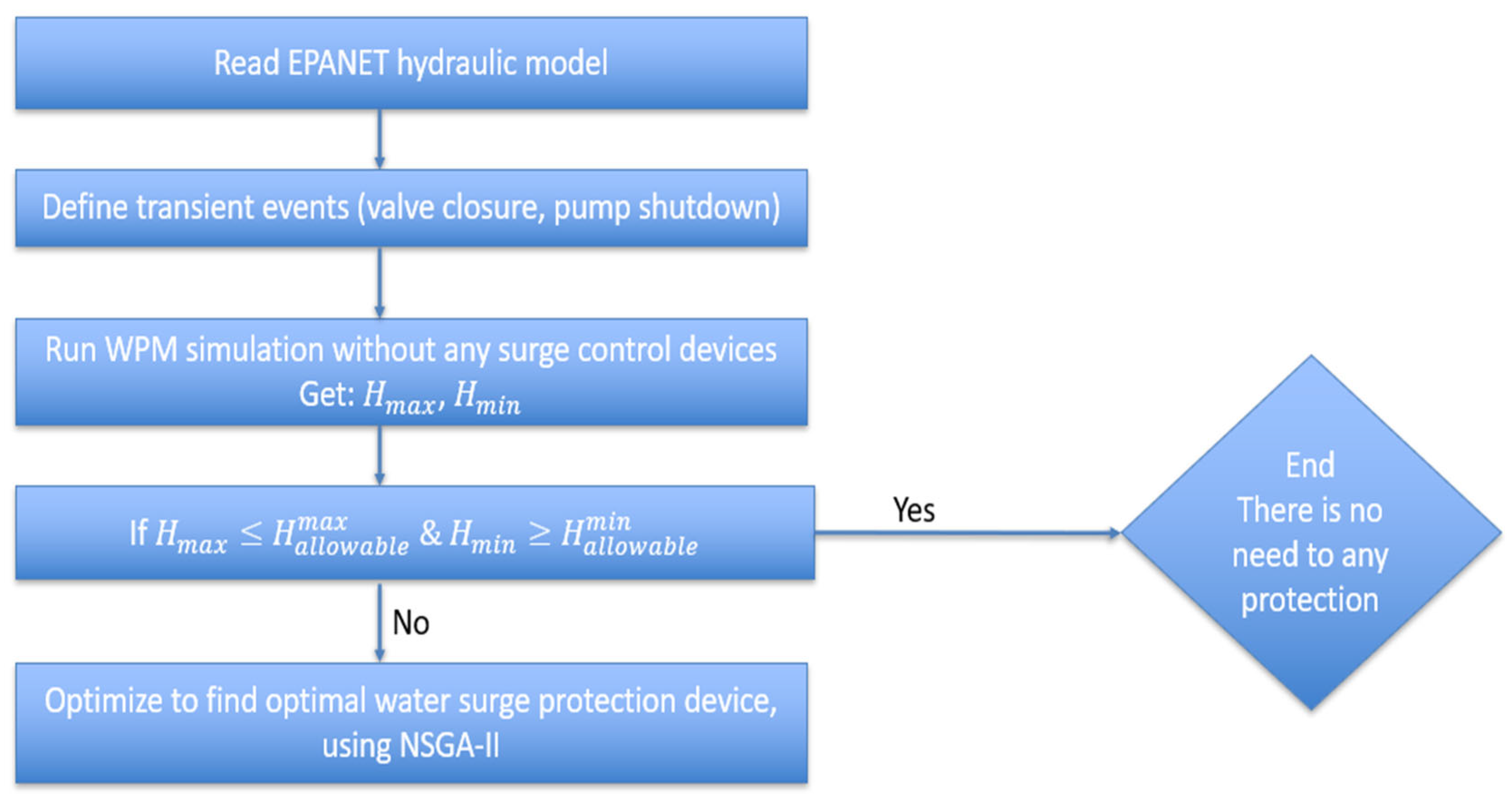
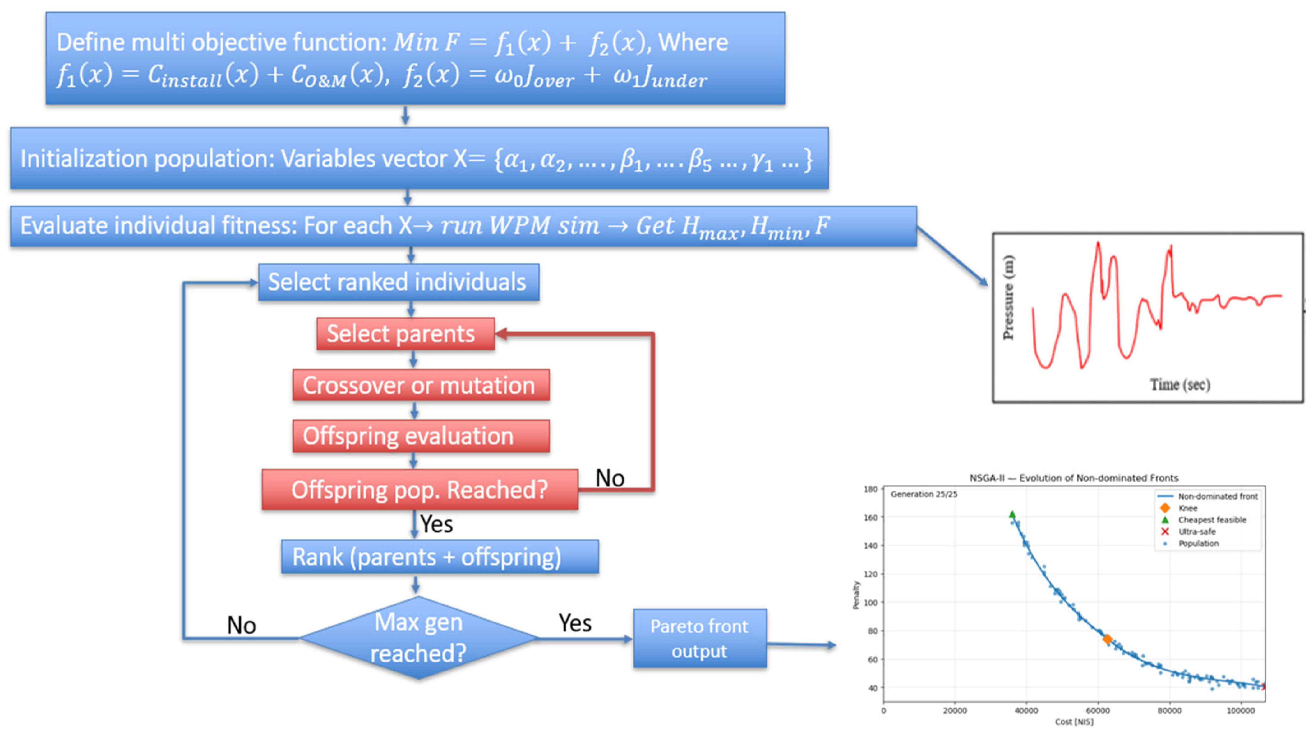
Figure 1 and Figure 2 below are a conceptual flowchart of this proposed simulation–optimization framework.

3.4. The Multi-Objective Function

We want to minimize two objectives: total installation cost of surge protection devices and a hydraulic penalty due to pressure violations. So the problem is described in Equation (14):

$$Min \{f_{\mathit{cost}}\left(x\right), f_{\mathit{pen}}\left(x\right)\}$$

(14)

Let x be the decision vector:

$$x=(b_{av}, b_{ot}, b_{bl}, b_{rv}, V_{av}, d_0, \varnothing , K, A_t, H_{t0}, C_{th}, V_b, H_{pre}, d_{ov}, K_b, D_v, H_{set}, t_{open}, t_{hold}, t_{closed}, C_d)$$

(15)

The definition of each variable is summarized in

Table 1. Decision variable description.

Symbol	Description	Units	Device
$b_{av}$	Air vessel activation (1 = on, 0 = off)	-	Air vessel
$b_{ot}$	Open surge tank activation (1 = on, 0 = off)	-	Open tank
$b_{bl}$	Bladder tank activation (1 = on, 0 = off)	-	Bladder
$b_{rv}$	Relief valve activation (1 = on, 0 = off)	-	Relief valve
$V_{av}$	Air vessel volume	${\mathrm{m}}^3$	Air vessel
$d_0$	Orifice/connection diameter	m	Air vessel
$\varnothing$	Air–water volume ratio/precharge coefficient	-	Air vessel
$K$	Polytropic exponent	-	Air vessel
$A_t$	Tank cross-sectional area	${\mathrm{m}}^2$	Open tank
$H_{t0}$	Initial water level	m	Open tank
$C_{th}$	Throttling coefficient	-	Open tank
$V_b$	Bladder tank volume	${\mathrm{m}}^3$	Bladder tank
$H_{pre}$	Precharge head	m	Bladder tank
$d_{ov}$	Orifice/connection diameter	m	Bladder tank
$K_b$	Polytropic exponent	-	Bladder tank
$D_v$	Relief valve diameter	m	Relief valve
$H_{set}$	Valve set pressure (opening head)	m	Relief valve
$t_{open}$	Opening time	s	Relief valve
$t_{hold}$	Fully open hold duration	s	Relief valve
$t_{closed}$	Closing time	s	Relief valve
$C_d$	Discharge coefficient	-	Relief valve

. These variables describe the activation state and physical/operational characteristics of all surge protection devices considered in the optimization framework.

3.4.1. Objective 1—Total Installation Cost

Each device contributes a cost only if it is activated:

$$f_{\mathit{cost}}\left(x\right)=b_{av}\hspace{0.17em}{C}_{av}\left(V_{av}\right)+b_{ot}\hspace{0.17em}{C}_{ot}(A_t,H_{t0})+b_{bl}\hspace{0.17em}{C}_{bl}\left(V_b\right)+b_{rv}\hspace{0.17em}{C}_{rv}\left(D_v\right)$$

(16)

The device costs are modeled as size-dependent functions, where each cost scales with the corresponding storage or structural volume (and with nominal diameter in the case of the relief valve). Let $k_{av}$, $k_{ot}$, $k_{bl}$, and $k_{rv}$ denote the unit cost coefficients; the cost laws are written as follows:

$$C_{av}\left(V_{av}\right)=k_{av}{V}_{av}$$

(17)

$$C_{ot}\left(A_t,H_{t0}\right)=k_{ot}{A}_t{H}_{to}$$

(18)

$$C_{bl}\left(V_b\right)=k_{bl}\hspace{0.17em}{V}_b$$

(19)

$$C_{rv}\left(D_v\right)=k_{rv}\hspace{0.17em}{D}_v$$

(20)

where $V_{av }$ and $V_b$ are the air vessel and bladder tank volumes, $A_t{H}_{t0}$ is the effective construction volume of the open surge tank, and $D_v$ is the relief valve diameter. The coefficients $k_{av}$, $k_{ot}$, $k_{bl}$, and $k_{rv}$ were obtained from the Dekel website (https://www.dekel.co.il, accessed on 15 December 2025) and expressed in NIS, but can be easily updated to reflect local market conditions without changing the optimization framework.

3.4.2. Objective 2—Hydraulic Penalty Function

The hydraulic penalty quantifies deviations from safe pressure limits during the full transient event simulated by the Wave Plan Method.

For node $i$ at time step $j$,

$$\mathrm{\Delta }{H}_{i,j}^{+}=max(0, H_{i,j}\left(x\right)-H_i^{max})$$

(21)

$$\mathrm{\Delta }{H}_{i,j}^{-}=max(0, H_i^{min}-H_{i,j}\left(\mathit{x}\right))$$

(22)

The total penalty is as follows:

$$f_{\mathit{pen}}(x)=\sum _{i\in \mathcal{N}}\sum _{j\in \mathcal{T}}\left[{\omega }_i^{+}\right(\mathrm{\Delta }{H}_{i,j}^{+}{)}^2+{\omega }_i^{-}\left(\mathrm{\Delta }{H}_{i,j}^{-}{)}^2\right]\mathrm{\Delta }t$$

(23)

where $H_{i,j}\left(x\right)$ is the pressure head value at each time step which comes from the WPM transient simulation, $H_i^{max},{ H}_i^{min}$ are allowable head limits, ${\omega }_i^{+},{ \omega }_i^{-}$ are weighting coefficients, and $\mathrm{\Delta }t$ is the simulation time step.

The final multi-objective function is described in Equation (14).

3.5. Constraints

The optimization problem is subject to a set of hydraulic, physical, and operational constraints that ensure feasibility of both the surge protection devices and the transient hydraulic response computed by the Wave Plan Method. These constraints are classified into three categories: (i) hydraulic safety constraints, (ii) physical bounds on decision variables, and (iii) operational and logical constraints related to device behavior.

3.5.1. Hydraulic Safety Constraints

For every node $i$ and every time step $j$ in the WPM transient simulation, the instantaneous piezometric head must satisfy

$$H_i^{min} \le H_{i,j}\left(x\right) \le H_i^{max}$$

(24)

where $H_i^{min}$ is the minimum allowable head (to prevent cavitation, vapor cavity formation, and column separation) and $H_i^{max}$ is the maximum allowable head (to prevent pipe rupture and overpressure damage).

Although violations are penalized through the hydraulic penalty function, the optimization must still satisfy global feasibility by keeping the system within physically meaningful bounds. For relief valves, an additional hydraulic condition, which ensures the valve opens only when the local head exceeds its set pressure, applies

$$H_{i,j}\left(\mathit{x}\right)\ge H_{set}\Rightarrow Q_v>0$$

(25)

3.5.2. Open Surge Tank Constraints

Activation constraints

$$A_{st}^{min}{y}_{ot}\le A_{st}\le A_{st}^{max}{y}_{ot}$$

(26)

$$H_{st}^{min}{y}_{ot}\le H_{st}\le H_{st}^{max}{y}_{ot}$$

(27)

If the tank is active ($y_{ot}=1$), its cross-section area and initial water level must lie within allowable design ranges. If the tank is inactive ($y_{ot}=0$), the constraints collapse to zero so the variables do not influence the simulation.

Water level existence

$$-M(1-y_{ot})\le h^{\left(n\right)}\le M{y}_{ot},\forall n$$

(28)

When the tank is active, the water level $h^{\left(n\right)}$ must be physically defined. When inactive, these constraints are disabled through Big-M.

Tank water level dynamics (continuity)

$$\mid h^{(n+1)}-h^{\left(n\right)}-{\displaystyle \frac{\mathrm{\Delta }t}{2A_{st}}}(Q_{\mathrm{conn}}^{\left(n\right)}+Q_{\mathrm{conn}}^{(n+1)})\mid \le M(1-y_{ot}),\forall n$$

(29)

The tank water level changes according to inflow/outflow through the connection pipe.

This enforces the mass-balance equation as follows:

$$A_{st}{\displaystyle \frac{dh}{dt}}=Q_{\mathit{conn}}$$

(30)

Tank junction head consistency

$$-M(1-y_{ot})\le H_P^{\left(n\right)}-h^{\left(n\right)}\le M(1-y_{ot}),\forall n$$

(31)

Because the open tank is exposed to the atmosphere, the hydraulic head at the connection node must equal the water surface elevation $h^{\left(n\right)}$.

Physical water level limits

$$0\le h^{\left(n\right)}\le H_{st}+M(1-y_{ot}),\forall n$$

(32)

The water level cannot be negative and cannot exceed the tank height.

3.5.3. Bladder Tank Constraints

Activation constraints

$$V_b^{min} y_{bl}\le V_b\le V_b^{max}{ y}_{bl}$$

(33)

$$H_0^{min}{ y}_{bl}\le H_0\le H_0^{max }{y}_{bl}$$

(34)

The bladder tank volume and initial water level must be within design limits only if the device is selected.

Air pocket existence

$$0\le V_g^{\left(n\right)}\le M{ y}_{bl}$$

(35)

$$0\le P_g^{\left(n\right)}\le M y_{bl}, \forall n$$

(36)

The compressed air volume and pressure must remain non-negative when the bladder tank is active.

Polytropic gas law

$$\mid P_g^{\left(n\right)}(V_g^{\left(n\right)}{)}^k-C_b\mid \le M(1-y_{bl}),\forall n$$

(37)

The air pocket obeys the polytropic relationship shown in Equation (38) below:

$$P_g{V}_g^k=\mathrm{constant}.$$

(38)

Big-M deactivates this constraint when the device is not used.

Physical volume bounds

$$0<V_g^{\left(n\right)}\le V_b+M(1-y_{bl}),\forall n$$

(39)

The air volume cannot exceed the total internal tank volume and must remain positive.

Mass continuity at device junction

$$\mid V_g^{(n+1)}-V_g^{\left(n\right)}+{\displaystyle \frac{\mathrm{\Delta }t}{2}}(Q_{\mathrm{conn}}^{\left(n\right)}+Q_{\mathrm{conn}}^{(n+1)})\mid \le M(1-y_{bl}),\forall n$$

(40)

A change in air volume corresponds exactly to the water entering or leaving the tank.

3.5.4. Closed Air Vessel Constraints

Activation constraints

$$V_{av}^{min}{y}_{av}\le V_{av}\le V_{av}^{max}{y}_{av}$$

(41)

$$0\le \varphi \le y_{av}$$

(42)

$$d_o^{min} y_{av}\le d_o\le d_o^{max}{ y}_{av}$$

(43)

The vessel volume, precharge ratio, and orifice diameter must lie in feasible ranges if the vessel is installed.

Air pocket state variables

$$0\le V_g^{\left(n\right)},P_g^{\left(n\right)}\le M y_{av}$$

(44)

Air pressure and air volume exist only when the air vessel is active.

Polytropic compression law

$$\mid P_g^{\left(n\right)}(V_g^{\left(n\right)}{)}^k-C_{av}\mid \le M(1-y_{av})$$

(45)

The compressed air pocket must satisfy the polytropic equation unless the device is inactive.

Air volume physical bound

$$0<V_g^{\left(n\right)}\le V_{av}+M(1-y_{av})$$

(46)

The air pocket must remain within vessel limits.

Mass continuity

$$\mid V_g^{(n+1)}-V_g^{\left(n\right)}+{\displaystyle \frac{\mathrm{\Delta }t}{2}}(Q_{\mathrm{conn}}^{\left(n\right)}+Q_{\mathrm{conn}}^{(n+1)})\mid \le M(1-y_{av})$$

(47)

Air volume changes match the water flow entering/exiting the vessel.

3.5.5. Relief Valve Constraints

Activation constraints

$$D_v^{min}{y}_{rv}\le D_v\le D_v^{max}{y}_{rv}$$

(48)

$$H_{\mathrm{set}}^{min}{y}_{rv}\le H_{\mathrm{set}}\le H_{\mathrm{set}}^{max}{y}_{rv}$$

(49)

Valve diameter and set pressure must lie within allowable ranges if the valve is used.

Node continuity (valve junction)

$$\mid Q_{P1}^{\left(n\right)}-Q_{P2}^{\left(n\right)}-Q_v^{\left(n\right)}\mid \le M(1-y_{rv}),\forall n$$

(50)

Flow leaving the pipeline must equal the relief valve discharge.

Node pressure consistency

$$\mid H_{P1}^{\left(n\right)}-H_{P2}^{\left(n\right)}\mid \le M(1-y_{rv})$$

(51)

The valve connects two adjacent nodes that share a hydraulic head.

Valve opening logic (binary $b_v^{\left(n\right)}$)

Valve opens only when

$$H_P^{\left(n\right)}>H_{\mathit{set}}$$

(52)

In constraint form,

$$H_P^{\left(n\right)}-H_{\mathit{set}}\ge -M(1-b_v^{\left(n\right)})+M(1-y_{rv})$$

(53)

$$H_P^{\left(n\right)}-H_{\mathit{set}}\le M{b}_v^{\left(n\right)}-\epsilon +M(1-y_{rv})$$

(54)

If pressure exceeds the set level, the valve must open. If not, the valve must remain closed.

Valve discharge equation

$$\mid Q_v^{\left(n\right)}-C_d{A}_v\sqrt{2g(H_P^{\left(n\right)}-H_{\mathrm{out}})}\mid \le M(1-b_v^{\left(n\right)}+1-y_{rv})$$

(55)

When the valve is open, flow must follow the standard orifice discharge equation.

When closed, the constraint is disabled.

Non-negativity

$$Q_v^{\left(n\right)}\ge 0$$

(56)

The valve cannot draw water into the system; it only releases excess pressure.

4. Case Study

To evaluate the performance of the proposed WPM–NSGA-II optimization framework, two transient hydraulic scenarios were modeled, each representing a realistic surge event in a pressurized water transmission system. Both case studies were constructed as simplified benchmark networks that capture the essential dynamics of water hammer while allowing full control over device placement and operational parameters. All simulations were performed using the Wave Plan Method (WPM) for transient propagation and the NSGA-II algorithm for multi-objective optimization. The selected case studies were chosen to represent typical transient-prone configurations in water distribution systems, including different system scales, boundary conditions, and dominant transient sources. Although limited in number, these examples capture common design challenges and allow the general behavior of the optimization framework to be evaluated under contrasting hydraulic conditions.

4.1. Case Study 1—Valve Closure

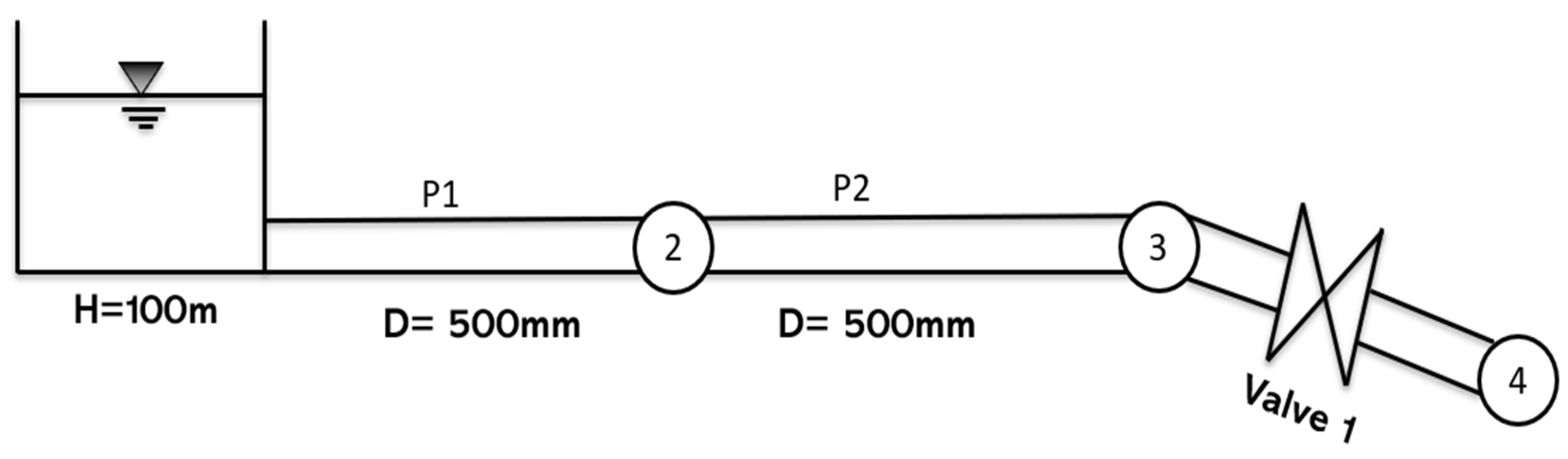
The first case study investigates a simple gravity-driven transmission system subjected to a downstream valve closure. The system consists of a constant-head reservoir supplying water through two steel pipeline sections connected in series to a terminal valve and a consumer node. This configuration represents a common layout in hillside conveyance systems, where rapid valve operations can generate significant pressure surges. The layout of the case study is shown in Figure 3. The upstream reservoir provides a constant hydraulic head of 100 m, feeding water into two 500 mm diameter steel pipes, denoted as P1 and P2. These pipes are connected sequentially and discharged toward a downstream valve (node N3) located near the consumer node (N4). Pipe P1’s length is 1.2 km, Pipe P2’s length is 2.4 km, the downstream flow demand is 50 m³/h, the Darcy–Weisbach roughness coefficient for all pipes is f = 0.017, and the wave celerity is a = 1000 m/s, representative of steel pipelines with typical elastic properties.

This case study focuses on pressure surges generated by rapid downstream valve closure. Such events create steep positive-pressure waves that propagate upstream and may exceed the allowable pressure limits of the pipeline. This case serves as a benchmark test for positive-pressure transients in simple transmission systems and establishes a baseline for evaluating the effectiveness of the optimization framework.

4.1.1. Simulation Results

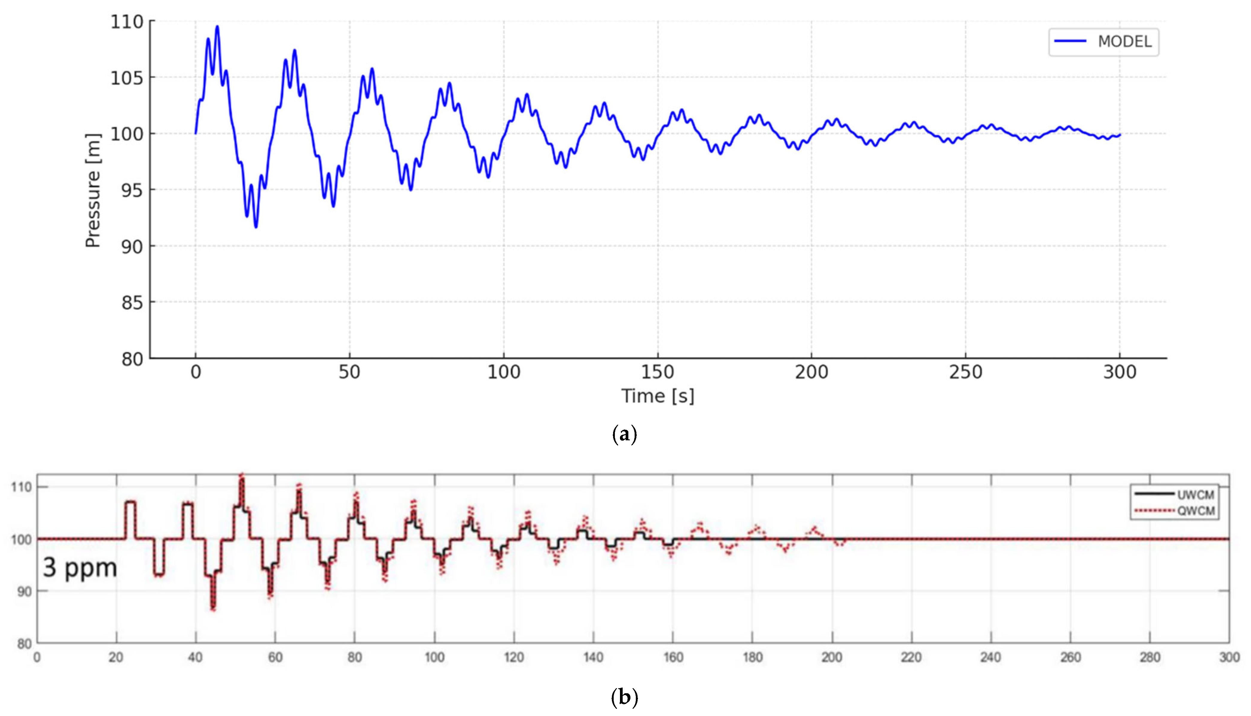
The pressure response was evaluated at node N3, identified as the most sensitive location during the valve-closure transient. Figure 4 presents the simulated pressure trace obtained using the developed Wave Plan Method (WPM) solver. To verify the correctness of the implementation, the results were compared against the classical analytical–numerical solution reported by Wood in the book of surge analysis for the same benchmark system and with Zeidan [8,18]. Studies [19,20] are also relevant to this work although using a different approach. Figure 4a shows this verification, where the pressure plot is for three pulses per minute (3 ppm).

These pulses are a direct consequence of the valve’s actions.

The comparison demonstrates excellent agreement: both responses exhibit nearly identical oscillation frequency, comparable peak and trough pressures, and a consistent damping envelope over time. This strong correspondence validates the numerical accuracy of the WPM implementation and confirms that the solver faithfully reproduces the core physics of water hammer propagation. Such validation is essential, as it ensures that the transient simulations used within the optimization framework are reliable and representative of the expected system behavior.

4.1.2. Optimization Results

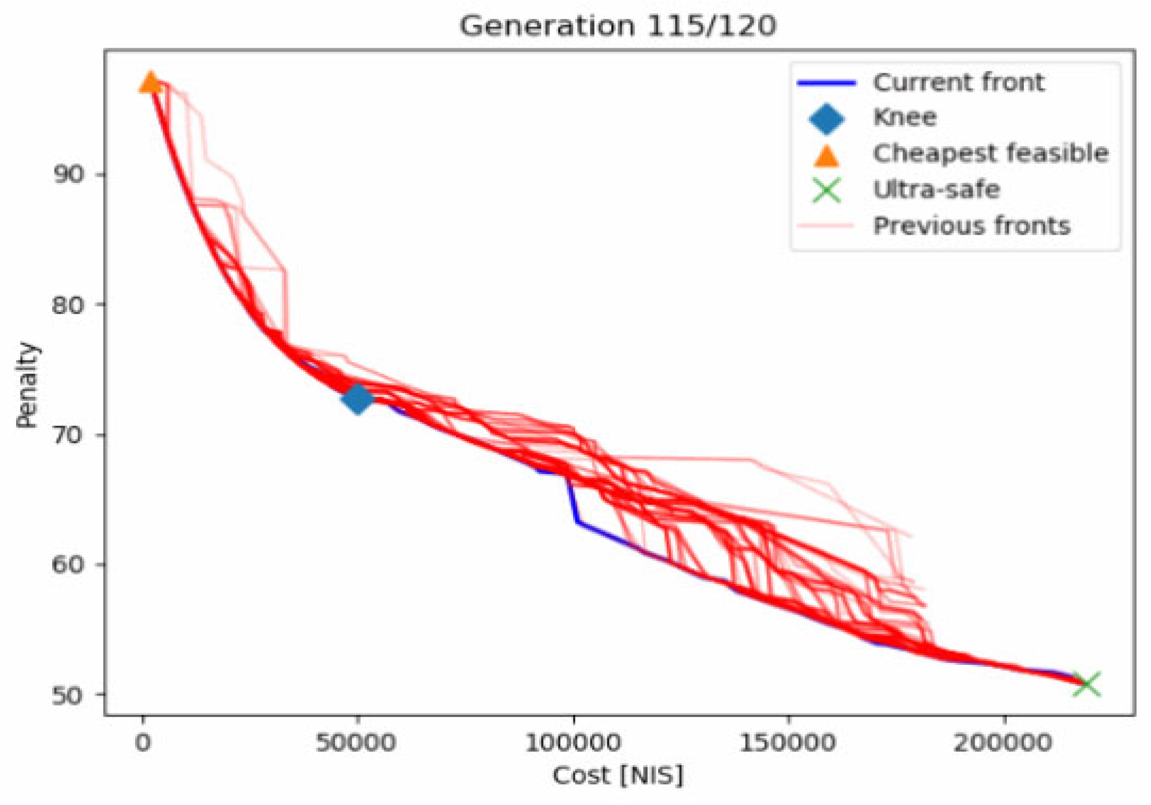
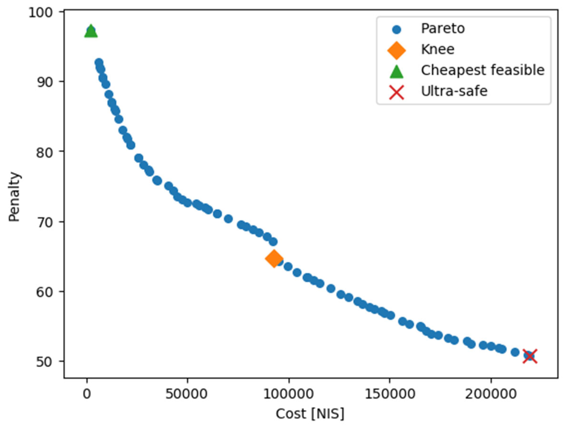
The NSGA-II algorithm was executed for 120 generations, minimizing the total device cost and the hydraulic penalty. During the evolutionary process, the Pareto front gradually expanded and improved, demonstrating the typical convergence behavior of NSGA-II. Early generations produced scattered, high-cost solutions with limited hydraulic benefit. By Generation 20, the algorithm began forming a coherent front, covering a wide range of cost–penalty combinations. At Generation 120, a well-shaped and stable Pareto curve was obtained, clearly revealing the trade-off between investment and hydraulic protection. The progress of the fronts in Figure 5 shows that the optimization successfully explored the design space and concentrated solutions around the most hydraulically effective regions. While Figure 6 shows the final generation pareto front, where the representative solutions extracted from it are described in

Table 2. Representative solutions extracted from the final Pareto front.

Solution Type	Devices Installed	Cost (NIS)	Penalty	Description
Cheapest Feasible Solution	Relief valve only	22,000	97.24	This solution eliminates cavitation but leaves relatively large pressure deviations.
Knee-Point Solution	Bladder surge tank	92,792	64.67	This design provides the best cost–performance balance, significantly improving transient behavior while keeping the investment moderate.
Ultra-Safe Solution	Air vessel + open surge tank + bladder tank	219,250	50.76	This configuration yields the lowest penalty, but at a very high cost, delivering only marginal improvement beyond the knee point.

.

The combined simulation–optimization framework successfully identified a complete spectrum of feasible surge protection designs. The knee-point solution (Recommended), represented by a single bladder surge tank at node N3, delivers substantial hydraulic improvement at a fraction of the cost of multi-device configurations. This demonstrates that the method provides effective engineering decision support, balancing safety and cost in transient control.

4.1.3. Comparison Between Open Surge Tank and Bladder Surge Tank at Node N3

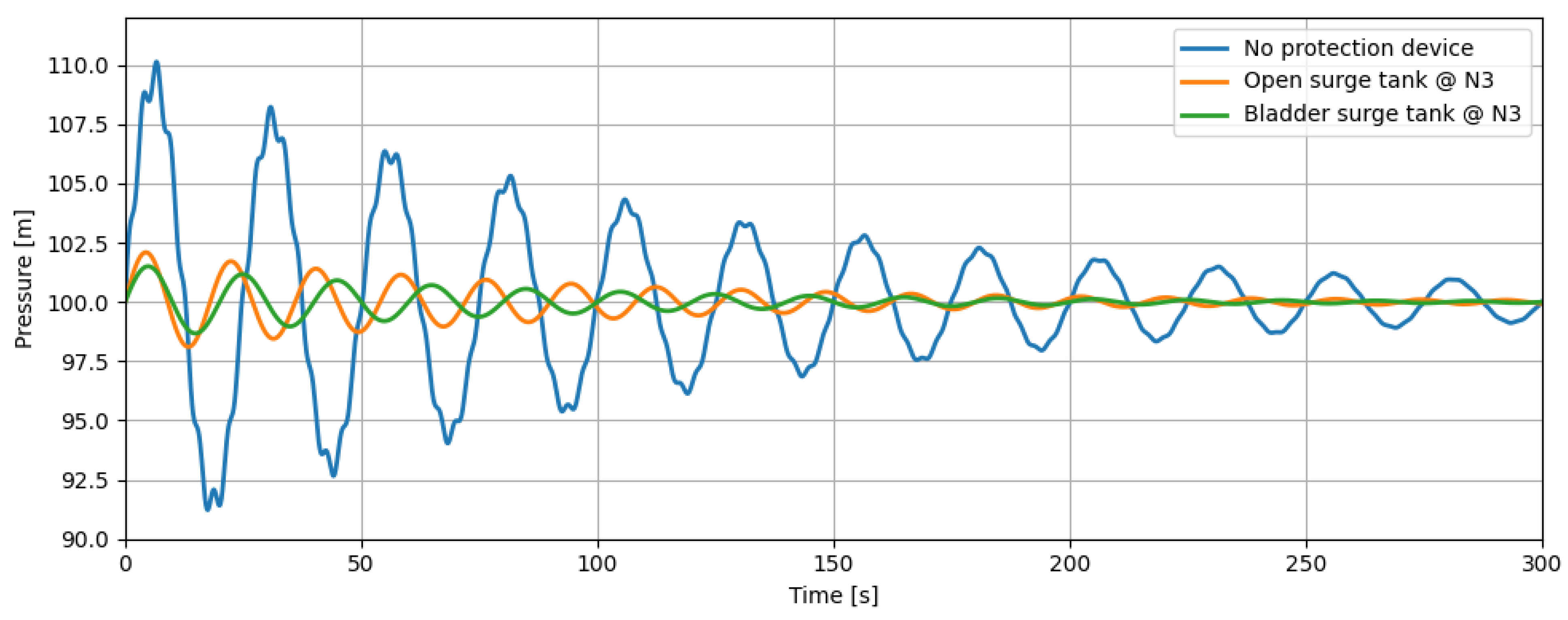
To further evaluate the hydraulic effectiveness of different surge protection devices, the pressure response at node N3 was simulated for two configurations: an open surge tank and a bladder (closed) surge tank. As shown in Figure 7, both devices significantly attenuate the transient oscillations following the valve-closure event; however, their behavior differs in amplitude reduction and damping rate. The open surge tank provides strong initial damping by allowing rapid mass exchange through the free water surface, but its response is less elastic, resulting in slightly larger pressure excursions during the early cycles. In contrast, the bladder surge tank—which relies on the compressibility of a trapped air cushion—produces a more uniform and smoother attenuation of the oscillations. This elastic air pocket absorbs and releases energy more gradually, yielding smaller peak pressures and a faster convergence toward steady-state conditions.

Overall, the results indicate that while both devices are effective at moderating the surge event, the bladder surge tank delivers superior damping performance, particularly in reducing extreme pressure spikes and minimizing long-term oscillations. These differences help explain why the bladder surge tank emerged as the recommended (knee-point) solution in the optimization results.

4.2. Case Study 2—Pump Trip

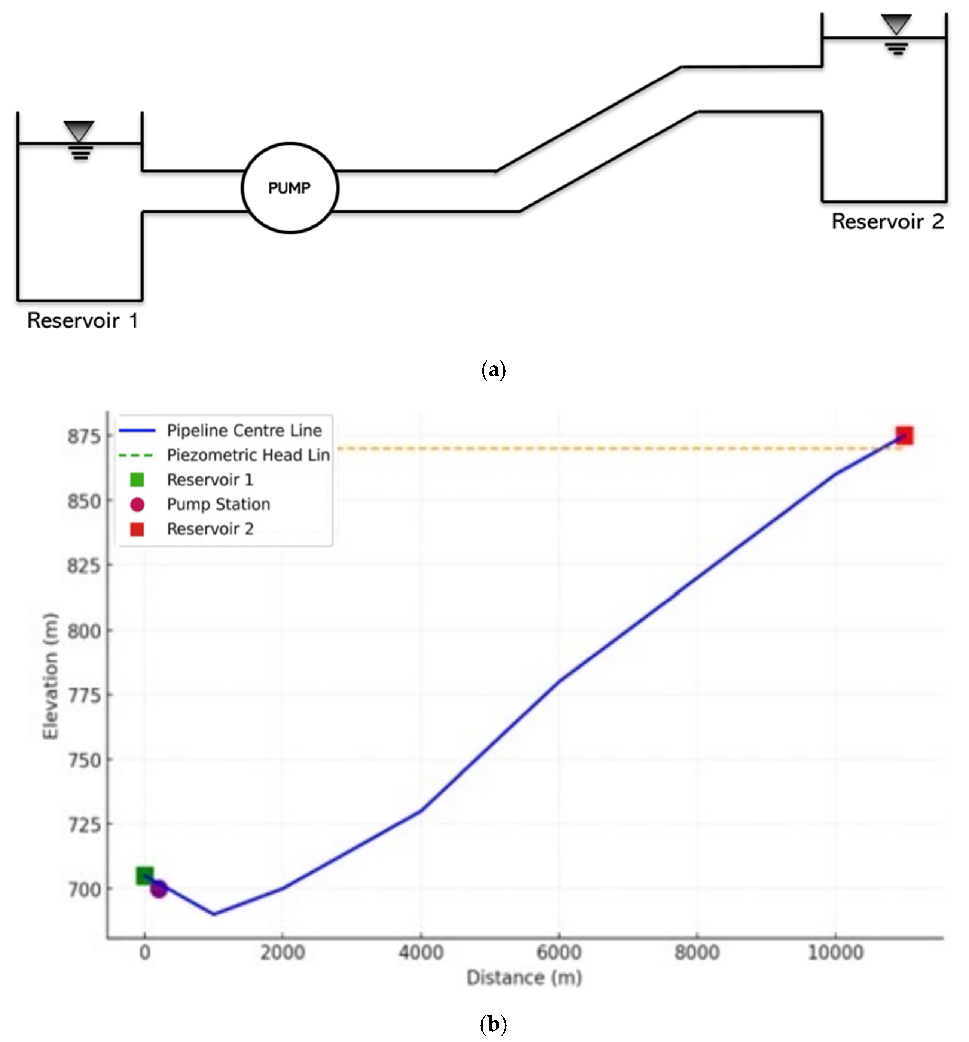
Figure 8 shows that the system consists of two reservoirs connected by a long rising main. The upstream reservoir supplies water to a pumping station, which then conveys the flow through more than 10 km of pipeline toward the downstream reservoir. The first part of the pipeline is nearly flat, while the second part climbs steeply, creating a large elevation difference between the two reservoirs. The pumps must overcome this significant static lift under normal operating conditions. The pipeline has a diameter of 1200 mm, carries a discharge of 1.3 m³/s, and exhibits a wave speed of about 1000 m/s. Three pumps operate in parallel, and the steep back section of the pipeline makes the system highly sensitive to rapid changes in flow. Because the line connects two reservoirs with a high head difference and a long, steep profile, it is especially vulnerable to pump-trip events. A sudden shutdown causes a sharp deceleration of the flow, which may trigger negative pressures near the upstream section and high upsurges near the downstream end. This makes the system a suitable real-world case for analyzing and optimizing water hammer protection strategies. The parameters of the pump station system are listed in

Table 3. Pump station parameters.

Parameter	Value
Reservoir 1 water level (m)	711.00
Reservoir 2 water level (m)	867.00
Pipe diameter (mm)	1200
Pipe length (km)	10.40
Flow discharge (m3/s)	1.30
Wave speed (m/s)	1000
Roughness coefficient	0.011
Quantity of pumps	3
Rated speed (r/min)	1480
Pump head (m)	165.57
Motor power (kW)	1250

below.

4.2.1. System Without Any Protection Device

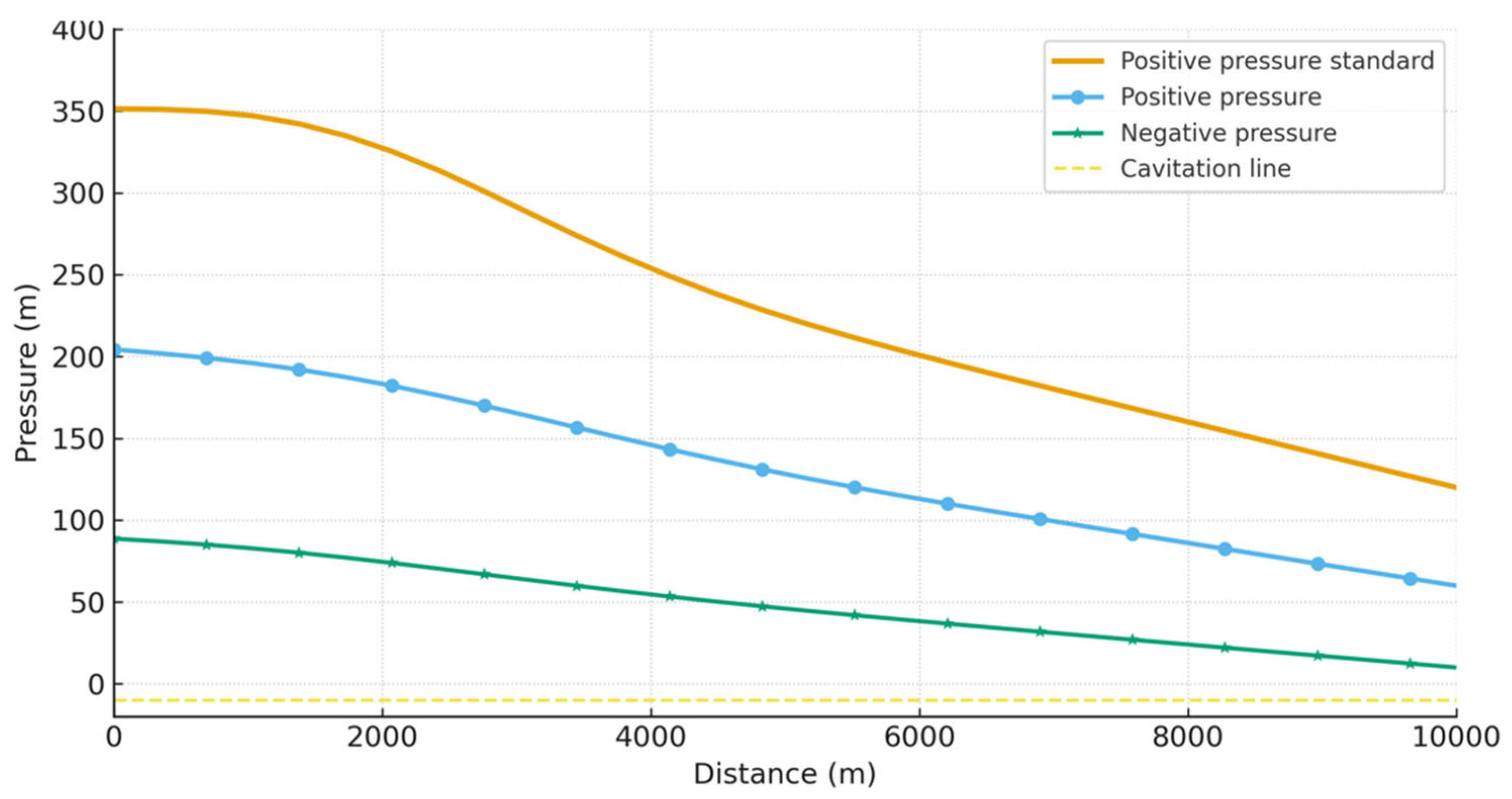
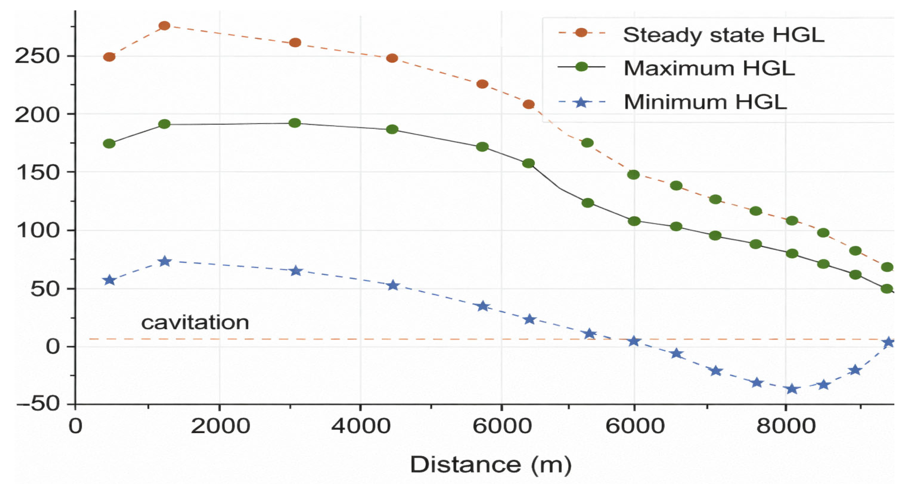
The pump-trip simulation shows an immediate pressure drop at the pump discharge that subsequently propagates along the rising main. The resulting maximum and minimum pressure envelopes along the pipeline are presented in Figure 9. Pressures below vapor pressure are shown to indicate cavitation risk; however, column separation effects are not explicitly modeled in this study.

4.2.2. Optimization Results

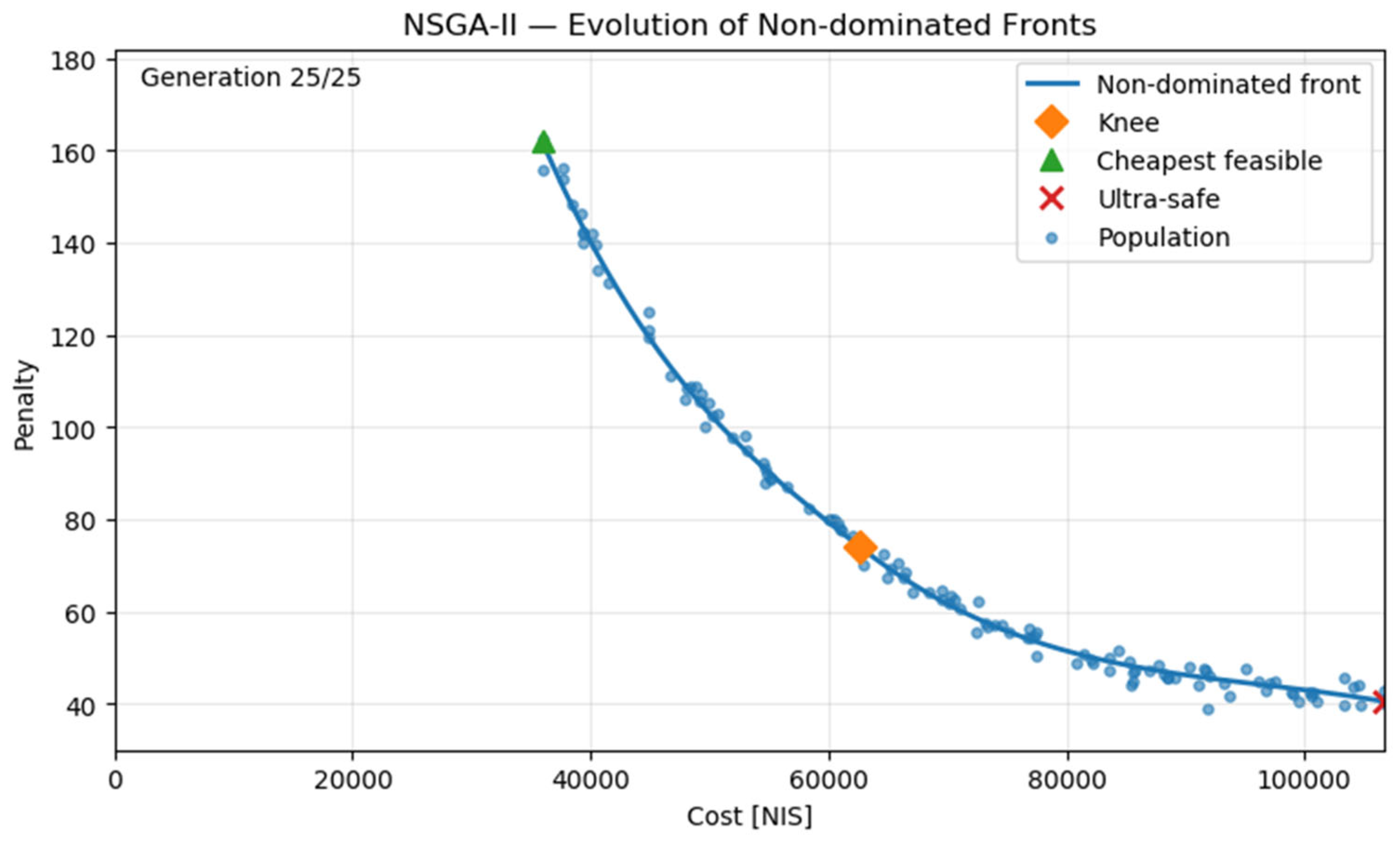
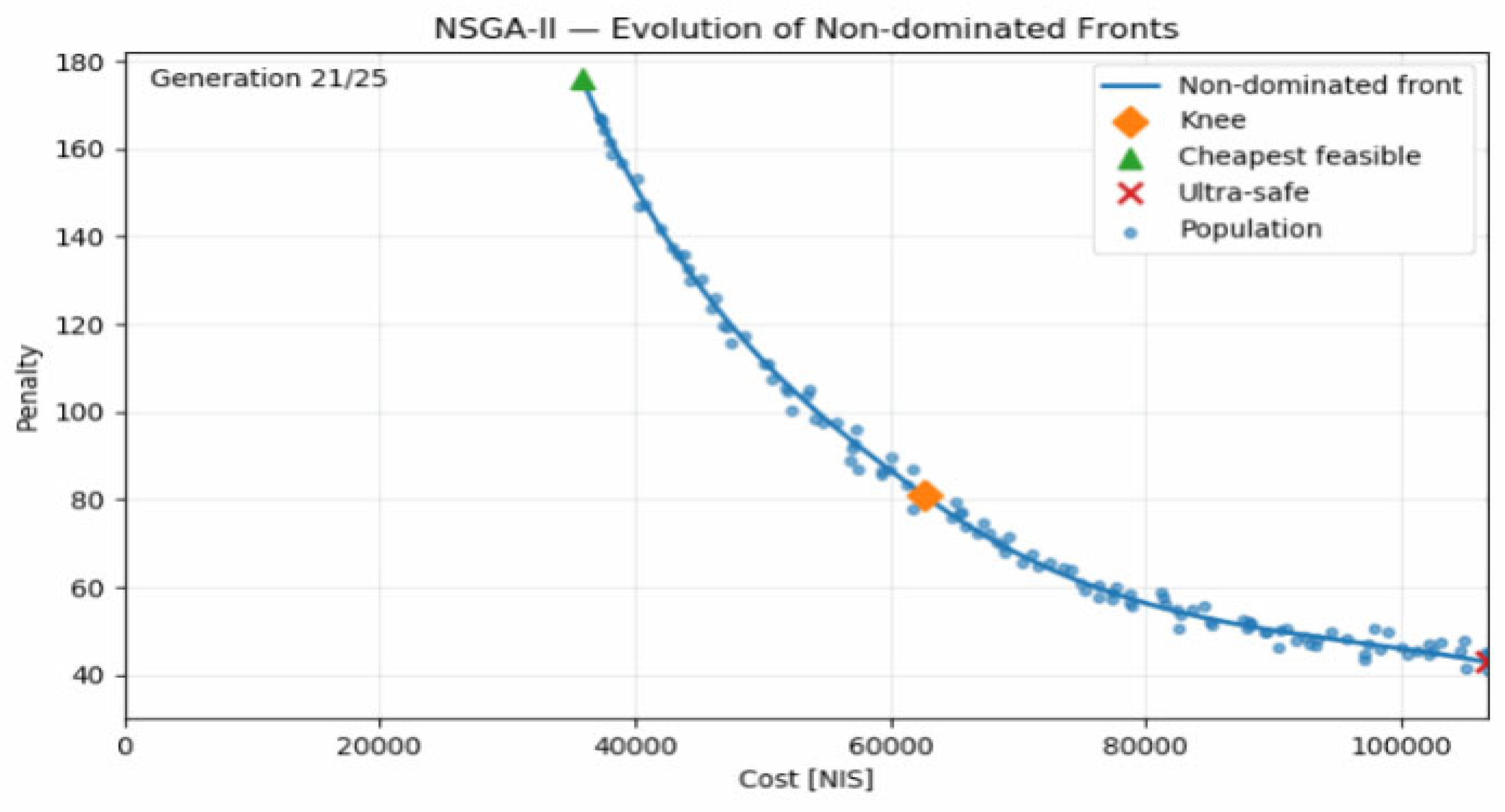
The NSGA-II algorithm was executed to identify the optimal surge protection configurations that balance installation cost with hydraulic performance. Figure 10 presents an animation of the Pareto front progress, and Figure 11 presents the final non-dominated front obtained after 25 generations, along with the full population of evaluated solutions. The Pareto curve exhibits a clear and smooth trade-off: lower-cost designs consistently result in higher penalty values, whereas improved hydraulic performance requires progressively higher investment.

At the low-cost end of the Pareto front lies the cheapest feasible solution, consisting of an air vessel (A) with a volume of 44.22 ${\mathrm{m}}^2$. This configuration is sufficient to prevent cavitation but still allows relatively large pressure deviations along the pipeline. It represents the minimum-cost option that satisfies the operational constraints, but its transient-pressure performance remains limited. Moving along the Pareto curve, the knee-point solution offers the best balance between performance and cost. This configuration combines air vessel A with a relief valve, significantly reducing both downsurge and upsurge magnitudes. The improvement in hydraulic behavior beyond this point becomes progressively smaller relative to the additional investment, making the knee-point solution the most cost-effective choice for practical engineering applications. At the rightmost part of the Pareto front is the ultra-safe solution, which employs air vessel (B) with a volume of 118.8 ${\mathrm{m}}^2$. This design achieves the lowest penalty among all evaluated configurations, effectively eliminating severe pressure fluctuations throughout the system. However, it comes at a substantially higher cost and provides only marginal performance gains beyond the knee-point solution. The shape parameters of air vessel A and B are shown in

Table 4. The shape parameters of air vessels A and B.

Parameter	Air Vessel A	Air Vessel B
Water depth (m)	2.5	1.5
Air height (m)	3	3
Cross-sectional area (m2)	8.04	26.4
Orifice diameter (m)	0.8	0.8
Elevation (m)	712.5	713.5
Volume (m3)	44.22	118.8

, and the setting parameters of the relief valve are shown in

Table 5. The setting parameters of the relief valve.

Parameter	Value
Location	+0.00
Diameter (mm)	100
Starting pressure (m)	180
Opening law	Linear opening in 0.5 s
Duration (s)	60
Closing law	Linear closing in 100 s

below.

4.2.3. Simulation Results

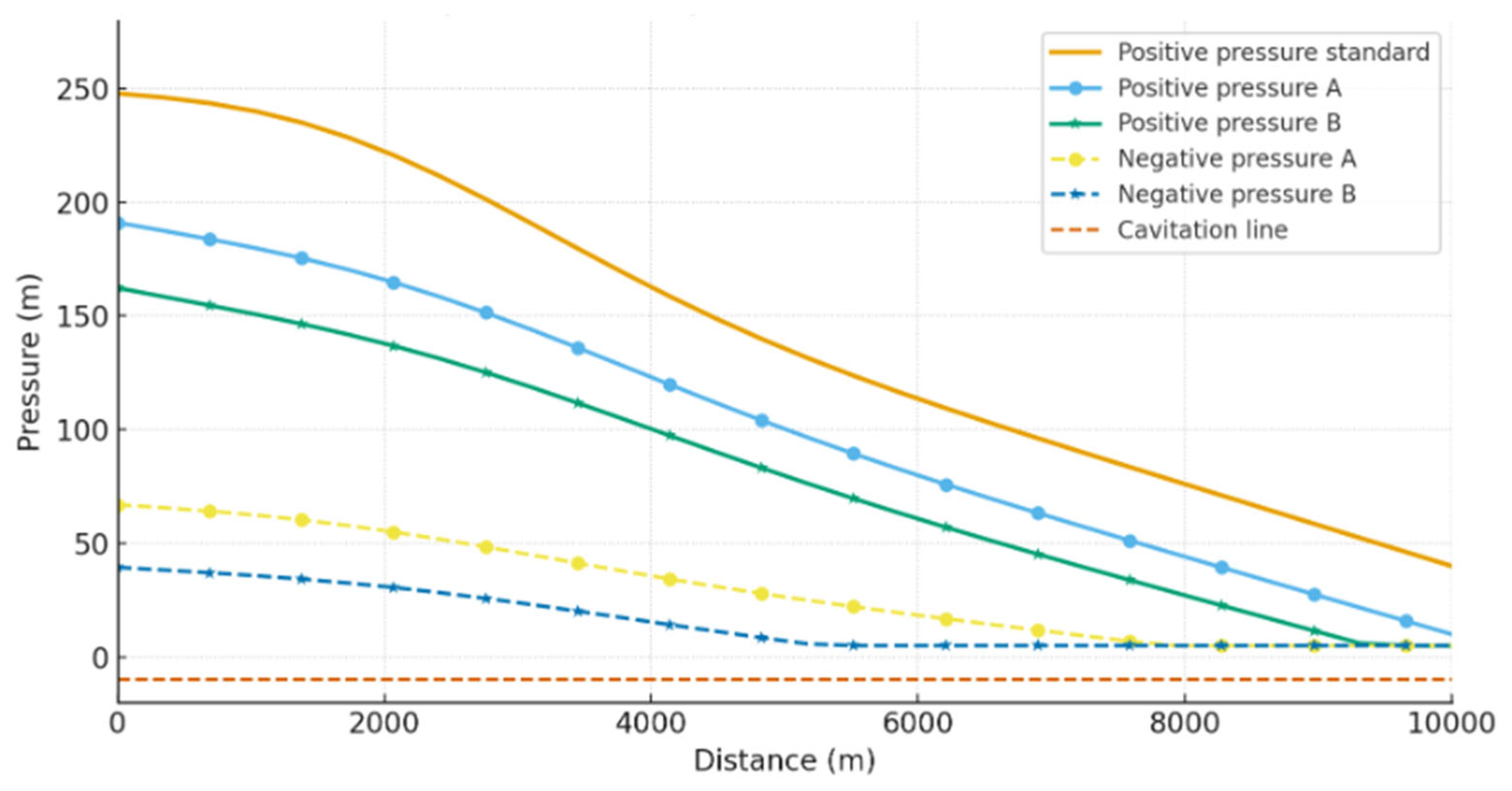
Based on the transient flow analysis, two distinct air vessel protection configurations—air vessel A and air vessel B—were developed. Following the pump-trip event, the hydraulic transient was simulated using the WPM, and the resulting enveloping curves of maximum and minimum pressures for each configuration are presented in Figure 12.

In air vessel A, the pipeline maintains adequate negative-pressure protection, but the resulting maximum pressure still exceeds the allowable positive-pressure limit.

Air vessel B improves both negative- and positive-pressure conditions, keeping pressures within the acceptable range. This improvement, however, requires a noticeably larger air vessel compared to method A. Overall, the results show that when using only an air vessel for surge protection, achieving negative-pressure safety is not enough; the vessel volume must be substantially increased to ensure compliance with both negative- and positive-pressure requirements.

To improve positive-pressure protection without increasing the size of the air vessel, the knee point offers a combined approach using air vessel A and a relief valve. The air vessel prevents negative pressures in the higher sections, while the relief valve which is installed downstream of the pump releases excess pressure during surges. The WPM simulation for the knee-point configuration gives a pressure envelope along the pipeline, as shown in Figure 13.

5. Conclusions

This study introduced an integrated WPM–NSGA-II framework for optimizing surge-control devices in pressurized water systems. By combining a detailed transient flow solver with a multi-objective evolutionary algorithm, the method successfully identified cost-effective and hydraulically reliable protection configurations. The resulting Pareto fronts clearly highlight the trade-off between investment and performance, showing that while low-cost solutions prevent cavitation, the knee-point designs provide the best balance between cost and surge mitigation. Ultra-safe options further reduce pressure extremes but with diminishing hydraulic benefits relative to their high cost. Overall, the framework offers a practical decision-support tool for designing surge protection systems and can be readily extended to more complex networks and operational scenarios.

References

1. Zhang, Q.; Tian, Z.; Lu, S.; Kang, H. Numerical Simulation of Water Hammer in Pipeline System Using Efficient Wave Tracking Method. Water Resour. Manag. 2023, 37, 4295–4310. [Google Scholar] [CrossRef] [Scilit]
2. Wood, D.J.; Dorsch, R.G.; Lightner, C. Digital Distributed Parameter Model for Analysis of Unsteady Flow in Liquid-Filled Lines; NASA: Washington, DC, USA, 1965. [Google Scholar]
3. Abdel-Gawad, H.A.A.; Djebedjian, B. Modeling Water Hammer in Viscoelastic Pipes Using the Wave Characteristic Method. Appl. Math. Model. 2020, 83, 353–366. [Google Scholar] [CrossRef] [Scilit]
4. Zhao, L.; Yang, Y.; Wang, T.; Zhou, L.; Li, Y.; Zhang, M. A Simulation Calculation Method of a Water Hammer with Multipoint Collapsing. Energies 2020, 13, 1103. [Google Scholar] [CrossRef] [Scilit]
5. Xing, L.; Sela, L. Transient Simulations in Water Distribution Networks: TSNet Python Package. Adv. Eng. Softw. 2020, 149, 102884. [Google Scholar] [CrossRef] [Scilit]
6. Xing, L.; Sela, L. An Overview of the Transient Simulation in Water Distribution Networks (TSNet). In World Environmental and Water Resources Congress 2020: Hydraulics, Waterways, and Water Distribution Systems Analysis–Selected Papers; ASCE: Reston, VA, USA, 2020; pp. 243–252. [Google Scholar] [CrossRef] [Scilit]
7. Lyu, J.; Zhang, J.; Wang, X.; Xu, T. A Combined Water Hammer Protective Method for Optimizing the Volume of the Air Vessel in Water Supply Systems. AQUA—Water Infrastruct. Ecosyst. Soc. 2021, 70, 1217–1230. [Google Scholar] [CrossRef] [Scilit]
8. Zeidan, M.; Ostfeld, A. Pressure Transient Utilization for Pipeline Particle Deposits Laceration. J. Hydraul. Eng. 2024, 150, 04023071. [Google Scholar] [CrossRef] [Scilit]
9. Eftekharian, S.E.; Shojafar, M.; Shamshirband, S. 2-Phase NSGA-II: An Optimized Reward and Risk Measurements Algorithm in Portfolio Optimization. Algorithms 2017, 10, 112. [Google Scholar] [CrossRef] [Scilit]
10. Kim, S.H. Design of Surge Tank for Water Supply Systems Using the Impulse Response Method with the GA Algorithm. J. Mech. Sci. Technol. 2010, 24, 629–636. [Google Scholar] [CrossRef] [Scilit]
11. Hur, J.; Kim, S.; Kim, H. Water Hammer Analysis That Uses the Impulse Response Method for a Reservoir-Pump Pipeline System. J. Mech. Sci. Technol. 2017, 31, 4833–4840. [Google Scholar] [CrossRef] [Scilit]
12. Wang, X.; Zhang, J.; Yu, X.; Shi, L.; Zhao, W.; Xu, H. Formula for Selecting Optimal Location of Air Vessel in Long-Distance Pumping Systems. Int. J. Press. Vessel. Pip. 2019, 172, 127–133. [Google Scholar] [CrossRef] [Scilit]
13. Zhou, Z.; Mu, Z.; Zhang, H.; Zhang, M.; Gu, Y.; Shi, X.; Zhao, B. Analysis and research on water hammer protection measures based on KY PIPE for long distance pumping station water transmission engineering with pump stoppage. Sci. Rep. 2025, 15, 158. [Google Scholar] [CrossRef] [Scilit] [PubMed]
14. Moghaddas, S.M.J.; Samani, H.M.V.; Haghighi, A. Transient protection optimization of pipelines using air-chamber and air-inlet valves. KSCE J. Civ. Eng. 2017, 21, 1991–1997. [Google Scholar] [CrossRef] [Scilit]
15. Ghidaoui, M.S.; Zhao, M.; McInnis, D.A.; Axworthy, D.H. A Review of Water Hammer Theory and Practice. Appl. Mech. Rev. 2005, 58, 49–76. [Google Scholar] [CrossRef] [Scilit]
16. Sharma, D.; Deb, K.; Kishore, N.N. Research Article Customized Evolutionary Optimization Procedure for Generating Minimum Weight Compliant Mechanisms. Eng. Optim. 2014, 46, 39–60. [Google Scholar] [CrossRef] [Scilit]
17. Lingireddy, S.; Wood, D.J. Surge Analysis and the Wave Plan Method: A Powerful, Accurate, and Stable Method for Water Hammer Studies; KYPipe LLC: Cary, NC, USA, 2021; Available online: https://kypipe.com/wp-content/uploads/2021/06/Surge-analysis-and-the-wave-plan-method-Intro.pdf (accessed on 30 January 2026).
18. Zhang, R.; Hu, J.; Wang, L.; Du, T.; Song, M.; Gao, H.; Mao, J.; Zhang, Z.; Fang, Y. Research on Water Hammer Protection in Coastal Drainage Pumping Stations Based on the Combined Application of Flap Valve and Sluice Gate. Water 2026, 18, 25. [Google Scholar] [CrossRef] [Scilit]
19. Mao, J.; Hu, J.; Wang, Y.; Gao, H.; Li, P.; Zhou, Y.; Xie, F.; Cui, J.; Hu, W. Study on Hydraulic Safety Control Strategies for Gravity Flow Water Supply Project with Long-Distance and Multi-Fluctuation Pressure Tunnels. Water 2025, 17, 2696. [Google Scholar] [CrossRef] [Scilit]
20. Aghaei, S.; Hamidi, M.; Malekpour, A.; Besharat, M. A Numerical Investigation into the Performance of Bypass Systems During Filling and Air Removal in Partially Drained Pipelines. Water 2025, 17, 1544. [Google Scholar] [CrossRef] [Scilit]
Figure 1. The WPM simulation flowchart.
Water 18 00455 g001
Figure 2. The NSGA-II optimization flowchart.
Water 18 00455 g002
Figure 3. Layout of the first case study.
Water 18 00455 g003
Figure 4. (a) Wave pressure obtained at node 3 after closing the valve. (b) Wave pressure obtained from the Zeidan [8] model.
Water 18 00455 g004
Figure 5. Pareto front progress.
Water 18 00455 g005
Figure 6. Pareto Front of the last generation.
Water 18 00455 g006
Figure 7. Pressure wave with open vs. closed surge tanks at node N3.
Water 18 00455 g007
Figure 8. (a) System layout. (b) Pipe center line, piezometric head line of the water supply system.
Water 18 00455 g008
Figure 9. Pressure envelope without any protection.
Water 18 00455 g009
Figure 10. Pareto front progress.
Water 18 00455 g010
Figure 11. Pareto front of the last generation.
Water 18 00455 g011
Figure 12. Pressure envelope curves for air vessels A and B.
Water 18 00455 g012
Figure 13. Pressure envelope curves for the knee-point solution.
Water 18 00455 g013