Spatial Dependence and Cluster Persistence in Drinking-Water Quality Risk: Municipal Evidence from the Department of Santander, Colombia, 2007–2020

Abstract

Drinking-water quality risk in Colombia is monitored through a single municipal indicator, the Water Quality Risk Index (IRCA), yet its spatial structure has not been examined. This study analyzes the 87 municipalities of the department of Santander between 2007 and 2020 (1202 municipality-year observations from SIVICAP/INS) using exploratory spatial data analysis. Global Moran’s I is estimated annually and by period, together with local indicators of spatial association (LISA), the Getis-Ord Gi* statistic, and a cluster-persistence test based on a binomial contrast with false discovery rate correction. Spatial dependence was positive and significant before 2014 (I = 0.113; p = 0.036) and became undetectable afterward (I = 0.046; p = 0.183); the share of IRCA variance attributable to spatial structure fell from 5.0% to 1.0%. The change in IRCA showed no detectable spatial clustering (I = 0.044; p = 0.198), suggesting, though not confirming, that the improvement did not spread through geographic contiguity. Cluster persistence reveals an asymmetry: eight municipalities maintain statistically significant low-risk cluster status after multiple-testing correction, led by Páramo (9 of 14 years) and San Gil (8 of 14), while no high-risk cluster survives that correction. The mean distance among the ten lowest-risk municipalities (≈60 km) remains below the departmental average (82.1 km) in both periods, whereas that among the ten highest-risk municipalities increases from 70.6 to 90.2 km. Finally, 2020 shows significant negative autocorrelation (I = −0.114; p = 0.040), coinciding with an increase in municipalities reporting an IRCA of zero (31 of 87, versus 1 in 2018), which suggests a disruption in the surveillance system rather than an actual change in water quality. Water safety consolidates territorially, whereas high risk does not form stable spatial structures.

1. Introduction

Access to safe drinking water remains one of the most consistent determinants of public health in low- and middle-income countries. The burden of disease attributable to unsafe drinking water, inadequate sanitation, and poor hygiene remains considerable, and falls disproportionately on rural populations [1]. In Latin America and the Caribbean, most people lacking at least a basic water service live in rural areas, so the problem is no longer primarily one of coverage but of the quality and continuity of the service actually delivered [2,3]. Colombia illustrates this transition: 74% of its population had access to a safely managed drinking-water service in 2024, but only 53% of monitored water bodies had good ambient quality and integrated water resources management implementation reached 41%, both indicators referring to 2023 [4].

Colombia offers unusually favorable conditions for studying the geographic dimension of this problem. Since 2007, Decree 1575 and Resolution 2115 have established a single national indicator of sanitary risk for water intended for human consumption, the Water Quality Risk Index (IRCA), calculated from noncompliance with microbiological and physicochemical parameters and reported for every municipality through the drinking-water quality surveillance information system (Sistema de Informacion de la Vigilancia de la Calidad del Agua para Consumo Humano, SIVICAP) of the Instituto Nacional de Salud [5,6,7]. The National Policy for Integrated Water Resources Management (PNGIRH), adopted in 2010, organized its implementation in phases, with a short-term horizon closing in 2014 [8]. Few countries in the region have a standardized, continuous municipal-level series of water risk spanning more than a decade around a clearly dated policy milestone.

The IRCA is the subject of active research. Recent studies have used it to document the gap between measured risk and citizens’ perception of water quality [9], and to examine the relationship between the territorial allocation of sector investment and quality outcomes, incorporating watershed structure and upstream–downstream relationships [10]. In parallel, spatial analysis of water quality has gained ground in the country, with studies that redesign monitoring networks in urban watersheds [11] or map physicochemical parameters in intermediate-sized cities [12]. However, these studies operate on sampling points or specific watersheds, not on the administrative unit where investment and surveillance decisions are made: the municipality.

Geography matters in this sector for concrete and verifiable reasons. Neighboring municipalities share watersheds and raw-water sources, are served by providers whose service areas overlap, participate in the same departmental water plan, and face similar costs in receiving technical assistance and transporting water-treatment inputs. Tobler’s observation that nearby units tend to resemble each other more than distant ones [13] translates, in this context, into a reasonable expectation: water risk should exhibit spatial dependence. Verifying whether that expectation holds, and whether it changes when policy changes, is an empirical question that has not been posed for the Colombian case.

The relevance of this question is supported by international experience. In East Africa, the detection of spatial clusters of unimproved water sources allowed priority areas for intervention to be identified from household surveys [14], and recent studies have mapped household water treatment in sub-Saharan Africa using hotspot analysis and spatial autocorrelation [15]. In India, global and local Moran’s I identified regional hotspots and coldspots of groundwater contamination relevant to drinking-water safety using the same queen-contiguity approach adopted here [16]. Closer to our design, a health-surveillance study in Ghana applied global Moran’s I, local indicators of spatial association, and the Getis-Ord Gi* statistic to district-level data from an administrative information system, and documented significant spatial clustering in the early years of the period that shifted toward a random distribution in the later years, a pattern discussed further in Section 3.1. That precedent is relevant because it shows that the loss of spatial structure in a surveillance indicator is a documented and interpretable outcome, not an artifact.

There is, moreover, a methodological reason to examine the spatial dimension. The evaluation of water policy typically relies on territorial averages, which summarize the level of risk but do not convey its geographic distribution. A decline in the departmental average is compatible with two very different scenarios: an improvement spread evenly, or an improvement concentrated in certain subregions while others remain lagging. Both scenarios produce the same aggregate figure and call for opposite policy decisions: general instruments in the first case, territorial targeting in the second. Distinguishing between them requires statistics that operate on the location of the units and not solely on their values.

This article poses three questions. First, does drinking-water quality risk in the municipalities of the department of Santander exhibit spatial dependence, and did that dependence change around the 2014 PNGIRH milestone? Second, where are the local clusters of high and low risk located, and did they shift between periods? Third, how persistent are those clusters over the fourteen years observed, once the fact that simultaneous statistical tests are being run across 87 municipalities is accounted for?

The contribution is threefold. Empirically, this is the first municipal-scale analysis of the spatial structure of the IRCA in a Colombian department, built on a cleaned fourteen-year panel of the official surveillance record. Methodologically, the article introduces a formal cluster-persistence test: rather than basing conclusions on the map of a single period, a common practice that, as shown below, does not withstand multiple-testing correction, the recurrence of each municipality is evaluated across independent annual cross-sections through a binomial contrast with false discovery rate control. On the policy side, the results directly inform the targeting criteria of departmental water plans, by distinguishing between conditions that aggregate territorially and conditions that do not.

2. Materials and Methods

2.1. Study Area

The department of Santander is located in northeastern Colombia, on the western flank of the Cordillera Oriental of the Andes. It borders Norte de Santander, Cesar, and Bolívar to the north; Antioquia to the west; and Boyacá to the south and east. Its territory covers 30,537 km², approximately 2.7% of the national area, and extends roughly 226 km east–west and 271 km north–south. The relief ranges from the Magdalena River valley, below 200 m a.s.l., to páramo peaks exceeding 4000 m. This altitudinal gradient shapes the availability and behavior of raw-water sources, as well as the logistical cost of transporting water-treatment inputs to mountain municipalities. Table 1 summarizes the main attributes of the study area.

Table 1. Summary of the study area.

Attribute	Value
Municipalities analyzed	87 (full universe, no sampling)
Departmental area	30,537 km2
Extent	226 km (E–W) × 271 km (N–S)
Elevation range	<200 to >4400 m a.s.l.
Municipal area	25 km2 (Palmar)–3179 km2 (Cimitarra); median 230 km2
Departmental population	1,929,120 (2007) → 2,287,806 (2020)
Municipal population (2020)	1457 (Palmar)–601,668 (Bucaramanga); median 5843
Concentration	4 metropolitan-area municipalities = 54.8% of the population
Composition (2020)	76.0% municipal and 24.0% scattered rural population centers
Density (2020)	median 31 inhab/km2; 6.5 (Gámbita)–3351 (Floridablanca)
Panel analyzed	1202 municipality-year observations (2007–2020)
Annual reporting coverage	82–87 municipalities
Mean IRCA 2014–2020	12.89; range 0.75–54.80

The unit of analysis is the municipality. The study includes the 87 municipalities that make up the department, that is, the entirety of Santander’s administrative units and not a sample. No selection criterion was applied, whether by population, rurality, or risk level, because the design is census-based: the full universe is analyzed. This decision avoids selection bias and is also a necessary condition of the method, since spatial autocorrelation statistics require a contiguous, closed set of units in order to construct the neighborhood matrix without artificial boundaries.

Santander’s municipalities differ markedly in size. Calculated from the polygons of the National Geostatistical Framework [17], the smallest municipality is Palmar, at 25 km², and the largest is Cimitarra, at 3179 km²: a ratio of 125 to 1. Median municipal area is 230 km² and the mean is 352 km², indicating a skewed distribution, with a few very large municipalities in the Magdalena valley set against a numerous group of small municipalities in the hillside areas.

This heterogeneity has a direct methodological consequence. When spatial units differ so much in size, the definition of “neighbor” ceases to be neutral: a large municipality tends to have more contiguity-based neighbors than a small one, regardless of the actual distance between their population centers. For this reason, the analysis does not rely on a single definition of neighborhood, but instead replicates all results under five different specifications of the spatial weights matrix (Section 2.3). Table 2 describes each specification.

Table 2. Specifications of the spatial weights matrix.

Specification	Neighborhood Definition	Mean Neighbors
Queen contiguity (main)	share at least one boundary point	5.22
K-nearest neighbors, k = 4	the 4 municipalities with the closest centroid	4.00
K-nearest neighbors, k = 5	the 5 closest	5.00
K-nearest neighbors, k = 6	the 6 closest	6.00
Distance band	centroid distance ≤ 35 km	12.85

According to DANE projections based on the 2018 census [18], Santander’s population grew from 1,929,120 inhabitants in 2007 to 2,287,806 in 2020. The distribution across municipalities is strongly asymmetric: the mean municipal population in 2020 was 26,297 inhabitants, but the median was only 5843, meaning that half of the department’s municipalities have fewer than six thousand inhabitants. The least populated municipality is Palmar (1457 inhabitants) and the most populated is Bucaramanga (601,668), a ratio of 413 to 1. Four metropolitan-area municipalities, Bucaramanga, Floridablanca, Girón, and Piedecuesta, concentrate 1,253,911 inhabitants, that is, 54.8% of the departmental population in 4.6% of the administrative units. In 2020, 76.0% of the population resided in municipal seats and 24.0% in scattered rural settlements and population centers. Density reflects the same contrast: the departmental median is 31 inhabitants per km², with a minimum of 6.5 in Gámbita and a maximum of 3351 in Floridablanca.

Because Santander’s provincial grouping changed during the study period, six historical provinces, eight provincial development hubs between 2005 and 2008, and seven administrative and planning provinces created by Ordinance 009 of 2019 [19], cluster locations are described using geographic coordinates rather than provincial names, which are neither stable over time nor equivalent across schemes.

The panel shows a substantial improvement in the distribution of risk between the two periods. Considering the municipal average, municipalities in the medium-risk category fell from 44 (51%) in 2007–2013 to 24 (28%) in 2014–2020, and those in the high-risk category from 14 (16%) to 4 (5%); conversely, no-risk municipalities rose from 3 (3%) to 18 (21%). In the last year observed, 49 municipalities (56%) reported an IRCA in the no-risk category. Dispersion, however, remains pronounced: in the 2014–2020 average, the minimum value corresponds to Bucaramanga (0.75) and the maximum to El Playón (54.80), a ratio of 73 to 1 between the department’s extremes.

2.2. Data Sources and Cleaning

The IRCA is Colombia’s official indicator of drinking-water sanitary risk, defined by Decree 1575 of 2007 [5] and regulated by Resolution 2115 of 2007 [6]. It is constructed from noncompliance with microbiological and physicochemical parameters in samples collected by health authorities, and is expressed on a scale from 0 to 100, where higher values indicate greater risk. The regulation defines five categories: no risk (0–5), low risk (5.1–14), medium risk (14.1–35), high risk (35.1–70), and sanitarily unviable (70.1–100). Annual municipal values come from SIVICAP, administered by the Instituto Nacional de Salud [7].

Municipal polygons correspond to DANE’s 2018 National Geostatistical Framework [17], projected to the MAGNA-SIRGAS/Colombia Bogotá system (EPSG:3116) for all calculations involving distances or areas.

Three operations were applied, all documented and reproducible. First, one observation exceeded the theoretical maximum of the index (El Playón, 2008) and was recoded as missing, consistent with a data-entry error in the source. Second, a displaced DANE municipal code for Girón in 2013 was detected and corrected; after correction, the panel contains no duplicate municipality-year pairs. Third, municipality-years without a report were not imputed. The resulting panel contains 1202 municipality-year observations for the period 2007–2020.

The analysis compares two windows delimited by 2014, the year marking the close of the PNGIRH’s short-term implementation phase (the policy itself was adopted in 2010): 2007–2013 (pre-2014 milestone) and 2014–2020 (post-2014 milestone). A sensitivity analysis using alternative cutoff years, reported in Section 3.2, confirms that the results are not an artifact of this specific choice. For inferential comparisons between periods, the municipal average of each window is used rather than annual values. The reason is that annual administrative indicators incorporate variation unrelated to the phenomenon of interest, changes in sampling intensity, in reporting completeness, or one-off events, and the seven-year average dampens that noise while preserving the cross-sectional geographic structure that is the object of the study.

2.3. Spatial Weights Matrices

Every spatial autocorrelation statistic requires first defining what “neighbor” means. That definition is not a technical detail: it is an assumption that shapes the result. For this reason, the analysis does not rely on a single matrix but on five alternative specifications.

Formally, the weights matrix W is an n × n matrix (87 × 87) whose element $w_{ij}$ measures the proximity between municipalities i and j, with $w_{ii}=0$ by convention.

The 35 km threshold corresponds to the minimum distance guaranteeing that no municipality is isolated. The Queen matrix produces a fully connected graph with no islands. All matrices are row-standardized, so that the nearest-centroid distance across the 87 municipalities ranges from 5.17 to 35.12 km (mean 12.37 km; median 11.20 km; 90th percentile 20.99 km); the 35 km value is set by a single municipality, Cimitarra, the department’s largest by area, whose nearest neighbor lies exactly at that distance. This confirms that the distance-band specification, the one specification of five that returns a qualitatively different result, is driven by a single geographically atypical unit rather than by a representative feature of the distance distribution.

Administrative contiguity is used as a proxy for shared institutional and logistical context rather than as a direct representation of hydrological connectivity: neighboring municipalities typically share overlapping service providers, participate jointly in the departmental water plan, and face comparable costs of technical assistance, but they do not necessarily share watersheds or raw-water intake points. Georeferenced data on shared basins, upstream–downstream relationships, and provider service areas at the municipal level are not available for the full 2007–2020 period; incorporating such hydrologically informed weights is identified in Section 4.5 as a direction for future research.

$$\sum _j{w}_{ij}=1 \mathrm{for} \mathrm{all} i$$

(1)

This standardization implies that a municipality’s neighborhood value is the average of its neighbors, not their sum; without it, municipalities with more neighbors would automatically carry greater weight in the statistic.

2.4. Global Spatial Autocorrelation

The question is direct: do municipalities with high water risk tend to be surrounded by other high-risk municipalities, or is risk distributed with no recognizable geographic pattern? Global Moran’s I [20] summarizes that tendency in a single number. If neighbors resemble each other more than would be expected by chance, the index is positive; if neighbors tend to differ, it is negative; if there is no pattern, it approaches its expected value under randomness.

Formally:

$$I={\displaystyle \frac{n}{S_0}}\cdot {\displaystyle \frac{{\displaystyle {\sum }_{i=1}^n}{\displaystyle {\sum }_{j=1}^n}{w}_{ij}\left(x_i-\stackrel{⃐}{x}\right)\left(x_j-\stackrel{⃐}{x}\right)}{{\displaystyle {\sum }_{i=1}^n}{\left(x_i-\stackrel{⃐}{x}\right)}^2}}, S_0={\displaystyle \sum _{i=1}^n}{\displaystyle \sum _{j=1}^n}{w}_{ij}$$

(2)

where n is the number of municipalities (87); $x_i$ is the mean IRCA of municipality i in the period considered; $\stackrel{⃐}{x}$ is the departmental mean; $w_{ij}$ is the spatial weight between i and j; and $S_0$ is the sum of all weights, equal to n under row standardization.

Under the null hypothesis of random spatial distribution, the expected value of the index is

$$E\left[I\right]={\displaystyle \frac{-1}{n-1}}={\displaystyle \frac{-1}{86}}=-0.0116$$

(3)

That is, the reference point is not zero but a slightly negative value.

The share of variance in the standardized indicator that is linearly associated with its spatial lag, reported in Section 3.2, is defined and computed as:

$$R_{spatial}^2={\left[corr(z, Wz)\right]}^2, \mathrm{w}\mathrm{h}\mathrm{e}\mathrm{r}\mathrm{e} z_i=\left(x_i-\overline{\mathrm{x}}\right)/s_x$$

(4)

where Wz is the spatial lag of the standardized indicator z. This quantity is the coefficient of determination (R²) of the bivariate ordinary least squares regression underlying the Moran scatterplot, and is mathematically distinct from Moran’s I itself: under row-standardized weights, I equals the slope of the regression of Wz on z, whereas $R_{spatial}^2$ equals the corresponding coefficient of determination. The two statistics answer different questions: I indicates the direction and intensity of spatial dependence, while $R_{spatial}^2$ indicates how much of the variance in the standardized indicator is linearly associated with its spatial lag.

2.5. Local Indicators of Spatial Association

The global index yields a single number for the whole department and, by construction, can conceal opposing situations that cancel each other out. Local indicators decompose that global value into a per-municipality contribution, making it possible to identify where clustering occurs.

Formally, the local Moran statistic for municipality i [21] is

$$I_i={\displaystyle \frac{\left(x_i-\stackrel{⃐}{x}\right)}{m_2}}\sum _j{w}_{ij}\left(x_j-\stackrel{⃐}{x}\right), m_2={\displaystyle \frac{{\displaystyle {\sum }_{i=1}^n}{\left(x_i-\stackrel{⃐}{x}\right)}^2}{n}}$$

(5)

where $m_2$ is the sample variance of the IRCA. The sum of the $I_i$ is proportional to the global index, so both statistics are mutually consistent.

Each municipality with a statistically significant $I_i$ is classified by comparing its own value with the average of its neighbors: High–High (high-risk cluster, or hotspot), Low–Low (low-risk cluster, or coldspot), and High–Low or Low–High (spatial outliers).

2.6. The Getis-Ord Gi* Statistic

The local Moran statistic and Gi* answer related but not identical questions: the former detects similarity between a municipality and its neighborhood, while the latter assesses whether the sum of values in a neighborhood, including the focal municipality itself, is abnormally high or low relative to the departmental total [22]. Using both makes it possible to verify that the detected clusters do not depend on the statistic chosen.

$$G_i^{\mathrm{*}}={\displaystyle \frac{\sum _j{w}_{ij}{x}_j-\stackrel{⃐}{X}\sum _j{w}_{ij}}{S\sqrt{\frac{n\sum _j{w}_{ij}^2 - {\left(\sum _j{w}_{ij}\right)}^2}{n - 1}}}}$$

(6)

where $\stackrel{⃐}{X}$ is the mean of the values and S is their standard deviation. The statistic is approximately standard normal: significant positive values identify clusters of high values; significant negative values, clusters of low values.

2.7. Permutation Inference

The statistics above do not admit a reliable theoretical distribution when the units are irregular in size and shape, as is the case here. Significance is therefore assessed through conditional randomization: the observed IRCA values are randomly reassigned across the 87 municipalities, the statistic is recalculated, and the procedure is repeated R times to empirically build the distribution under the null hypothesis.

$$p_{\mathrm{pseudo}}={\displaystyle \frac{M+1}{R+1}}, z_{\mathrm{sim}}={\displaystyle \frac{I_{\mathrm{obs}}-E\left[I_{\mathrm{perm}}\right]}{{\sigma }_{I_{\mathrm{perm}}}}}$$

(7)

where M is the number of permutations that produced a statistic equal to or more extreme than the one observed, and R is the total number of permutations. R = 99,999 permutations were used for period statistics and R = 9999 for the annual series, with a fixed seed to ensure reproducibility. Table 3 defines all parameters used throughout the article.

Table 3. Definition of the reported parameters.

Symbol	Name	What It Indicates	Range or Reference
I	Global Moran’s I	Intensity and sign of spatial dependence	Positive: clustering; negative: dispersion; reference E[I] = −0.0116
Ii	Local Moran	Contribution of municipality i to the global pattern	Sign defines the quadrant
Gi*	Getis-Ord	Concentration of high or low values in the neighborhood of i	Approximately N(0, 1)
z	Standardized score	Standard deviations between the observed and expected value under randomness	|z| > 1.96 ≈ significance at 5%
p	Pseudo p-value	Proportion of permutations with an equal or more extreme statistic	Significant if p < 0.05
wij	Spatial weight	Degree of neighborhood between i and j	Row-standardized
n	Spatial units	Municipalities analyzed	87
R	Permutations	Randomization repetitions	9999 or 99,999

2.8. Cluster Persistence Test

A cluster map corresponds to a single period and simultaneously evaluates 87 hypotheses, one per municipality. At a 5% significance level, roughly four municipalities would be expected to be significant by chance alone. Significance in a single map is therefore weak evidence. A municipality that appears as a cluster recurrently across successive annual cross-sections, by contrast, constitutes a considerably stronger signal.

LISA statistics are calculated independently for each of the fourteen years. Let $T_i$ be the number of years in which municipality i reported an IRCA, and $k_i$ the number of those years in which it was a significant cluster of a given type. Under the null hypothesis that significance arises by chance with probability $\alpha =0.05$ each year, the number of occurrences follows a binomial distribution, and the probability of observing at least $k_i$ is

$$P\left(K_i\ge k_i\right)={\displaystyle \sum _{j=k_i}^{T_i}}\left({\displaystyle \genfrac{}{}{0pt}{}{T_i}{j}}\right){\alpha }^j{\left(1-\alpha \right)}^{T_i-j}$$

(8)

Since this contrast is applied to all 87 municipalities, the false discovery rate is controlled using the Benjamini–Hochberg procedure [23]: p-values are ordered from smallest to largest, and the largest index k satisfying

$$p_{\left(k\right)}\le {\displaystyle \frac{k}{m}}q, m=87, q=0.05$$

(9)

is identified, with the null hypotheses corresponding to $p_{\left(1\right)}$ through $p_{\left(k\right)}$ rejected. The same procedure is applied to the period LISA maps to assess how many clusters survive the correction.

2.9. Software and Reproducibility

All computations were performed in Python 3.11 using the libpysal and esda libraries of the PySAL ecosystem [24], and geopandas for cartographic processing. Random seeds were fixed in all permutation procedures. The replication script, the specification of the weights matrices, and the exact cleaning rules are available in a public repository (Zenodo, https://doi.org/10.5281/zenodo.21708806) and allow the reported results to be fully reproduced.

3. Results

3.1. Annual Evolution of Spatial Autocorrelation

Before comparing periods, it is useful to examine the full year-by-year series, for two reasons: it verifies that the pre/post contrast does not depend on an arbitrary cutoff, and it exposes the year-to-year variability that justifies working with period averages in the main inferential analysis. Table 4 reports the annual results.

Table 4. Global Moran’s I of annual municipal IRCA, Santander, 2007–2020.

Year	n	I	z	p	Significance
2007	85	0.030	0.638	0.255	—
2008	82	0.156	2.430	0.011	**
2009	86	0.162	2.577	0.009	**
2010	83	0.128	1.971	0.031	*
2011	86	0.092	1.523	0.071	—
2012	85	0.023	0.528	0.286	—
2013	87	−0.002	0.146	0.413	—
2014	87	0.047	0.907	0.175	—
2015	87	0.101	1.718	0.051	—
2016	87	0.005	0.261	0.381	—
2017	87	0.075	1.333	0.098	—
2018	87	0.048	0.939	0.173	—
2019	86	0.095	1.646	0.064	—
2020	87	−0.114	−1.569	0.040	*

Notes: Queen contiguity, row-standardized weights, R = 9999 permutations, fixed seed. E[I] = −0.0116. ** p < 0.01; * p < 0.05. n = municipalities reporting each year.

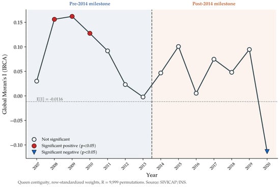
The series shows three successive regimes. Between 2008 and 2010, autocorrelation is positive and significant, with I values between 0.128 and 0.162: neighboring municipalities exhibited similar risk levels with a frequency that randomness does not explain. Between 2011 and 2013, the index declines monotonically until it nearly matches its expected value under randomness. From 2014 onward, the series fluctuates around low values without reaching significance, with the exception of the final year.

Several technical clarifications are important at this point. First, the reference point is not zero but E[I] = −0.0116; an observed value of 0.030, as in 2007, sits above that reference but within the range compatible with randomness. Second, p-values close to the conventional threshold are unstable. The year 2015 yields p = 0.051, just above 0.05; since inference is built through randomization, values this close to the threshold fluctuate with the seed and the number of permutations. For this reason, no significance is attributed to it, and the article’s argument does not rest on any single year. Third, annual coverage varies between 82 and 87 municipalities; for each year the weights matrix is recalculated, restricted to the units with data, so no fictitious neighborhoods are introduced, at the cost of statistical power varying slightly across years.

The pattern observed, significant clustering in the early years dissolving toward a random distribution in later years, is not anomalous. Ngmenbelle et al. [25] document the same sequence when analyzing health-surveillance indicators at the district level in Ghana with the same trio of statistics used here. The coincidence suggests that the loss of spatial structure in an administrative surveillance indicator is a recognizable phenomenon, not a peculiarity of the Colombian case. Figure 1 traces this trajectory.

Figure 1. Global Moran’s I of annual municipal IRCA, 2007–2020. Filled markers indicate pseudo p < 0.05 with R = 9999 permutations; the dotted line corresponds to the expected value under the null hypothesis; the dashed vertical line marks the 2014 cutoff.

3.2. Comparison Between Periods and Robustness to the Definition of Neighborhood

Period averages reduce sampling noise and allow for a more stable contrast. The question is whether the spatial structure detectable before 2014 remains detectable afterward (see Table 5).

Table 5. Global Moran’s I on period averages, under five neighborhood specifications.

Weights Matrix	Mean Neighbors	Pre-2014: I (p)	Post-2014: I (p)	Total: I (p)
Queen (main)	5.22	0.113 (0.036)	0.046 (0.183)	0.090 (0.068)
K-nearest, k = 4	4.00	0.098 (0.061)	0.076 (0.100)	0.092 (0.068)
K-nearest, k = 5	5.00	0.107 (0.035)	0.067 (0.099)	0.090 (0.057)
K-nearest, k = 6	6.00	0.087 (0.047)	0.065 (0.087)	0.080 (0.059)
35 km band	12.85	−0.010 (0.477)	−0.018 (0.479)	−0.029 (0.378)

Notes: p-values in parentheses. Queen: R = 99,999 permutations; others: R = 9999. Results significant at 5% shown in bold.

The results support two claims and not a third. The supported claims are that in 2007–2013, the spatial autocorrelation of the IRCA is distinguishable from randomness under three of the five neighborhood specifications; and that in 2014–2020 it is not distinguishable under any of them. The unsupported claim is that the two I values differ significantly from one another. No widely accepted standard test exists for contrasting the equality of two Moran’s I statistics computed on the same population at different times, precisely because the observations are not independent between periods: they are the same 87 municipalities. Accordingly, the claim is that spatial dependence ceased to be detectable, not that it declined by a statistically significant magnitude.

The four-neighbor specification retains a magnitude comparable to the main one (0.098 versus 0.113) but does not reach the conventional threshold. Reducing the number of neighbors causes each local average to be computed over fewer observations, which increases its variance and widens the distribution of the statistic under permutation. That the three specifications with five or more neighbors agree in detecting the signal strengthens the conclusion. This is why significance is lost at k = 4.

With a 35 km radius, each municipality has an average of 12.85 neighbors, more than double that under contiguity. The resulting index is negative and not significant in all three periods. This does not invalidate the previous results; it places them on a scale. The spatial dependence detected operates among adjacent municipalities, not among municipalities located tens of kilometers apart. When the neighborhood widens to cover a substantial portion of the department, the average of the neighbors approaches the departmental average and the statistic loses its discriminating power. This behavior is a manifestation of the modifiable areal unit problem in its scale dimension, and reporting it explicitly delimits the scope of the finding: the structure is local, not subregional.

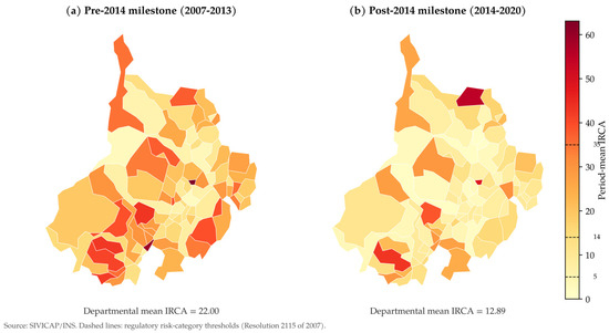
The squared correlation between the standardized indicator and its spatial lag ($R_{spatial}^2$, defined in Section 2.4) fell from 5.0% to 1.0% between periods. This figure guards against overinterpretation: geography was never the main determinant of water risk in Santander, since 95% of the variation across municipalities was already attributable, in the first period, to factors specific to each municipality rather than to its neighborhood. What the analysis documents is that this geographic component, always a minority share, fell to one-fifth of its original size. Figure 2 maps the period-mean IRCA for each municipality.

Figure 2. Mean drinking-water quality risk (IRCA) by municipality, Santander: (a) 2007–2013; (b) 2014–2020. Dashed lines on the color bar mark the regulatory category thresholds. Source: SIVICAP/INS; authors’ elaboration.

The 2014 milestone was adopted because it marks the close of the PNGIRH’s short-term implementation phase, not the year the policy itself was adopted (2010). To verify that the reported pattern does not depend on this specific choice, global Moran’s I was re-estimated for five alternative cutoff years (2012 through 2016) (see Table 6).

Table 6. Sensitivity of global Moran’s I to the choice of cutoff year.

Cutoff Year	Pre-Cutoff: I (p)	Post-Cutoff: I (p)
2012	0.142 (0.015)	0.042 (0.191)
2013	0.124 (0.025)	0.038 (0.207)
2014 (main)	0.113 (0.038)	0.046 (0.177)
2015	0.105 (0.045)	0.049 (0.161)
2016	0.105 (0.047)	0.030 (0.233)

Notes: Queen contiguity, row-standardized weights, R = 9999 permutations. Pre-cutoff window: 2007 through year − 1; post-cutoff window: cutoff year through 2020. The 2014 row therefore uses fewer permutations than the corresponding Queen-contiguity estimate in Table 5 (R = 99,999), which is why the p-values for the 2014 cutoff differ marginally between the two tables (0.036 vs. 0.038 pre-cutoff; 0.183 vs. 0.177 post-cutoff); the point estimates of I are identical. Bold values indicate results significant at the 5% level.

The qualitative pattern, significant positive autocorrelation before the cutoff and non-significant autocorrelation after it, holds across all five candidate years, confirming that the finding does not depend on the specific choice of 2014 as the breakpoint.

3.3. The Improvement Did Not Spread Geographically

The previous sections describe where risk was located. This question is different: where did the reduction occur? If the improvement had spread across contiguous territories, the change in IRCA should exhibit spatial clustering.

For the change between periods (Δ = 2014–2020 average − 2007–2013 average; mean = −9.11 points; standard deviation = 9.50):

$$I_{\mathsf{\Delta }}=0.044 z=0.836 p=0.198$$

(10)

No spatial structure is detected in the improvement. Municipalities that reduced their risk substantially and municipalities that reduced it only slightly are intermingled without forming clusters. The result is consistent with an improvement driven by factors operating above the municipal scale, reaching the entire territory regardless of each municipality’s location.

Failing to detect clustering does not equate to demonstrating its absence. With 87 units, the power to detect small values of I is limited, and weak clustering in the change could go unnoticed. What can be affirmed is that, if geographic diffusion of the improvement did occur, its intensity was smaller than that of the spatial dependence detected in the levels of the previous period, computed over the same population, with the same weights matrix and the same inference procedure.

3.4. Local Clusters, Multiple Testing, and Cross-Validation

As shown below (Table 7), no individual cluster on these single-period maps survives correction for multiple testing; this finding concerns the period-mean LISA maps specifically and is distinct from the year-by-year persistence test introduced in Section 3.5, where several clusters do survive correction.

Table 7. Significant local clusters (LISA, p < 0.05, R = 99,999).

	Pre-2014 (2007–2013)	Post-2014 (2014–2020)
High–High	3: Aguada (30.6), La Paz (29.9), Onzaga (25.3)	3: Jesús María (22.9), Suratá (17.0), La Belleza (13.6)
Low–Low	10 municipalities	8 municipalities
Spatial outliers	4	4
Total significant	17	15
Survive FDR correction	0	0

Notes: Mean municipal IRCA for the period shown in parentheses. Bold values indicate results significant at the 5% level.

Local indicators evaluate one hypothesis per municipality: 87 simultaneous contrasts. At a nominal 5% level, roughly 4.35 municipalities would be expected to be significant by chance even if no local structure existed at all.

The number of detected clusters far exceeds what would be expected by chance. Subjected to a binomial contrast, the excess is decisive: 17 of 87 versus 4.35 expected in the earlier period (p = 1.3 × 10⁻⁶) and 15 of 87 in the later period (p = 2.6 × 10⁻⁵). The combined reading is as follows: local structure exists in the territory, since the number of detected clusters cannot be attributed to chance, but the evidence from a single map is not enough to state with statistical confidence which individual municipalities constitute it. When the Benjamini–Hochberg correction is applied across the 87 contrasts, no municipality individually surpasses the threshold in either period. Both statements are simultaneously true: the first concerns the aggregate, the second each unit. This is the methodological reason why the persistence analysis constitutes the core of the article.

This comparison against the 4.35 expected count is presented only as an informal, descriptive check that the number of nominally significant local clusters exceeds what independent 5%-level tests would produce by chance; because neighboring LISA statistics are not spatially independent, by construction, since they share overlapping neighborhoods and the underlying spatial weights, this comparison is not a formally calibrated hypothesis test and should not be read as a substitute for the Benjamini–Hochberg correction that follows, which governs the substantive claims made in this article.

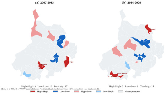
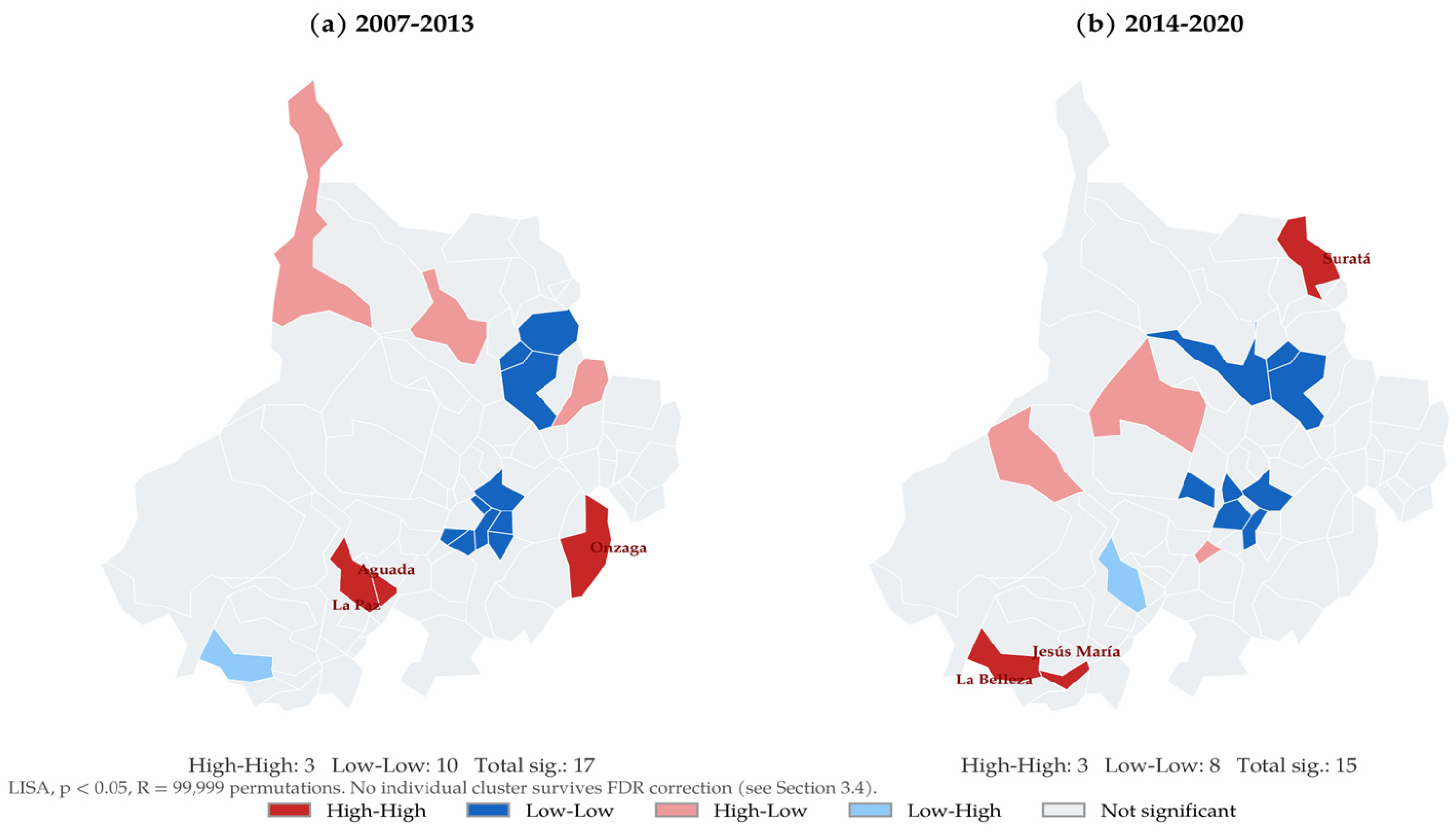
The three High–High clusters of the earlier period disappear entirely from the later set. Among Low–Low clusters, by contrast, San Gil, Piedecuesta, Floridablanca, and Páramo appear in both periods.

The Getis-Ord statistic identifies the same hotspots in both periods and adds La Belleza to the earlier set and La Paz to the later one. For coldspots, it detects 13 and 11 municipalities respectively, with substantial overlap. The discrepancies stem from the conceptual difference between the two statistics. That two statistics with different definitions converge on the same municipalities reinforces the conclusion that the clusters are not an artifact of the technique used. Figure 3 maps these clusters for both periods.

Figure 3. LISA cluster maps of period-mean IRCA (pseudo p < 0.05, R = 99,999): (a) 2007–2013; (b) 2014–2020. High–High clusters are labelled. The colour scheme was verified against simulated protanopia, deuteranopia and tritanopia ([26] model, colorspacious implementation) and remains distinguishable under all three conditions.

3.5. Cluster Persistence

Table 8 reports, for each municipality, the number of years as a significant cluster, the total years with a valid report, the binomial p-value, and whether the municipality survives Benjamini–Hochberg correction.

Table 8. Cluster persistence, 2007–2020.

Municipality	Years as Cluster	Years with Report	p (Binomial)	Significant After FDR
Low-risk clusters
Páramo	9	14	3.1 × 10−9	Yes
San Gil	8	14	8.9 × 10−8	Yes
Floridablanca	7	13	1.0 × 10−6	Yes
Cabrera	6	14	3.3 × 10−5	Yes
Piedecuesta	5	12	1.8 × 10−4	Yes
Confines	5	14	4.3 × 10−4	Yes
Valle de San José	5	14	4.3 × 10−4	Yes
Palmas del Socorro	4	14	4.2 × 10−3	Yes
High-risk clusters
La Belleza	4	12	2.2 × 10−3	No
La Paz	3	14	3.0 × 10−2	No
El Guacamayo	3	14	3.0 × 10−2	No
Contratación	2	14	1.5 × 10−1	No
Jesús María	2	14	1.5 × 10−1	No
Florián	2	14	1.5 × 10−1	No
Albania	2	14	1.5 × 10−1	No

Notes: Binomial contrast with α = 0.05 under the null hypothesis of chance significance; Benjamini–Hochberg correction with q = 0.05 across the 87 municipalities.

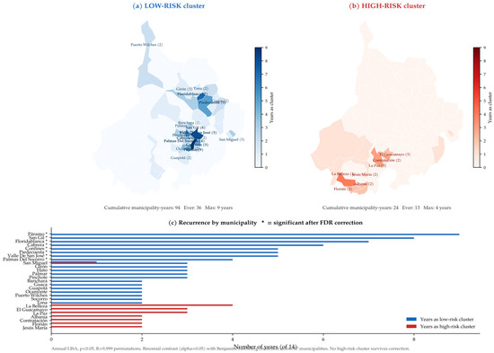
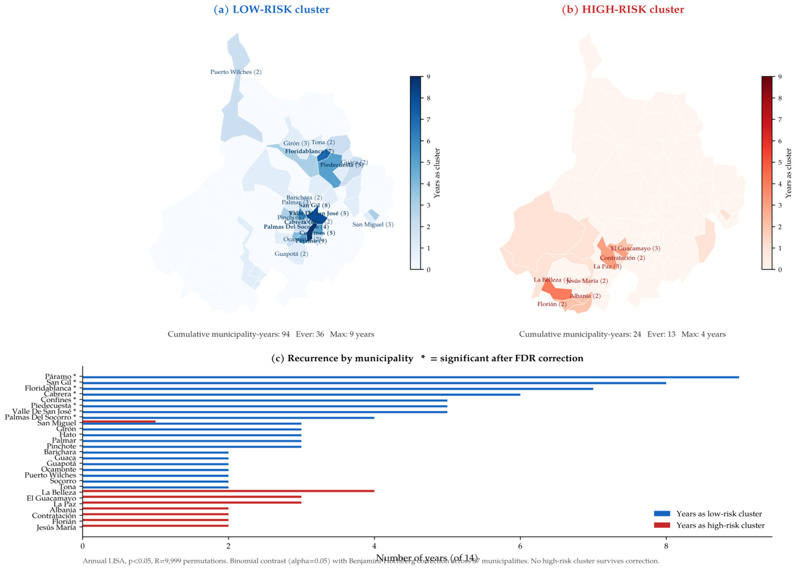
The contrast yields a sharp asymmetry: eight municipalities maintain statistically significant low-risk cluster status after controlling the false discovery rate, while no high-risk cluster reaches that threshold. The cumulative magnitudes reinforce the reading: 94 municipality-years in low-risk cluster status versus 24 in high-risk status; 36 municipalities reached the former condition at some point versus 13 the latter; and the maximum recurrence is nine years for low risk and four for high risk.

The binomial contrast assumes that the fourteen annual contrasts are independent of one another. This assumption does not strictly hold: a municipality’s IRCA in one year is related to that of the previous year. We estimated the first-order temporal autocorrelation of the municipal IRCA, obtaining a median of 0.210, and applying Bartlett’s correction (n_eff = T(1 − ρ)/(1 + ρ), with T = 14 and median ρ = 0.210) yields an approximate equivalent of 9.1 effectively independent years out of the 14 observed. The ratio n_eff/T = 9.1/14 = 0.650 was applied multiplicatively to both the observed count of significant years and the total number of years with a report; both scaled quantities were rounded down (floored) to the nearest integer, a conservative choice that avoids overstating the effective sample size, before evaluating the binomial test and reapplying the Benjamini–Hochberg correction. For Paramo (9 of 14 years), for example, this yields floored values of 5 of 9 years. Under that treatment, three municipalities retain significance as low-risk clusters, Páramo, San Gil, and Floridablanca, and no municipality retains it as a high-risk cluster. The central conclusion holds under both treatments, although the exact number of municipalities identified depends on the criterion adopted.

A single municipality, San Miguel, records both conditions over the course of the period: it was a high-risk cluster in 2009 and a low-risk cluster between 2017 and 2019. Examining its neighborhood explains the shift: the mean IRCA of its four neighbors, Macaravita, Capitanejo, Carcasí, and Enciso, fell from 42.85 to 1.16 points between the two moments, so the municipality moved from belonging to a high-risk neighborhood to belonging to a low-risk one without changing its relative position within it. The case illustrates that the documented reconfiguration operates on entire neighborhoods rather than on isolated municipalities, and that high-risk cluster status is not a permanent condition. Figure 4 maps the persistence counts and recurrence by municipality.

Figure 4. Persistence of annual LISA clusters, 2007–2020: (a) years as a low-risk cluster; (b) years as a high-risk cluster; (c) recurrence by municipality. The symbol * indicates significance after FDR correction. The colour scheme was verified for colour-vision deficiency as described in the note to Figure 3. Numbers in parentheses indicate years as a significant cluster.

3.6. The Geometry of Aggregation

The statistics above require familiarity with spatial inference. The mean distance between municipalities is a physical, directly interpretable quantity that allows the asymmetry to be verified without relying on distributional assumptions or weights matrices (see Table 9).

Table 9. Mean distance between municipal centroids, by number of municipalities considered.

Municipalities Considered	Pre: Lowest IRCA	Pre: Highest IRCA	Post: Lowest IRCA	Post: Highest IRCA
5	65.7 km	69.9 km	49.0 km	103.3 km
10	61.9 km	70.6 km	59.1 km	90.2 km
15	69.1 km	96.4 km	66.9 km	89.6 km
20	66.0 km	92.2 km	70.3 km	101.0 km

Note: Mean departmental distance between centroid pairs: 82.1 km.

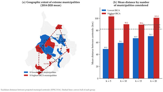
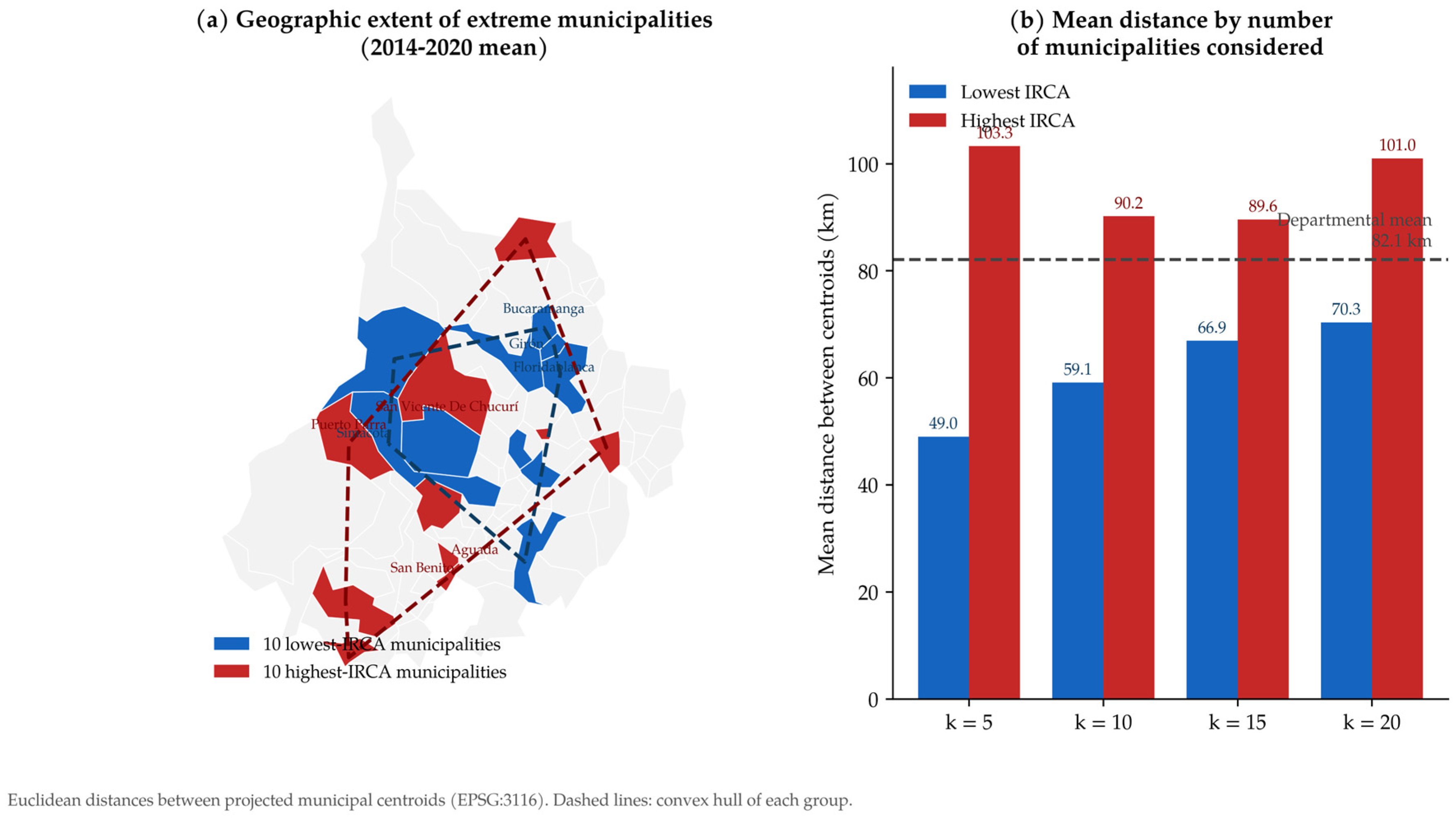
Under all four specifications and in both periods, lower-risk municipalities lie below the departmental average, while higher-risk municipalities exceed it consistently in the later period. The sharpest contrast corresponds to the five extreme municipalities after 2014: 49.0 km among the lowest-risk municipalities versus 103.3 km among the highest-risk ones.

The same conclusion follows from comparing the geographic extent occupied by each persistent group: the eight statistically significant coldspots are distributed across a band of 0.26° of longitude and 0.70° of latitude, while the eight municipalities with the greatest recurrence of high risk span 1.13° and 1.68° respectively, an area 4.3 times wider and 2.4 times taller. Low risk occupies a compact corridor in the center-east of the department; high risk is dispersed toward the west and southwest without forming a corridor. Figure 5 illustrates the geographic extent of each group and the mean inter-centroid distances.

Figure 5. Geometry of aggregation: (a) geographic extent of extreme municipalities in the 2014–2020 average, with the convex hull of each group; (b) mean distance between centroids by the number of municipalities considered. The dashed horizontal line in panel (b) indicates the departmental mean distance between centroid pairs (82.1 km).

3.7. The 2020 Anomaly

Table 10 contrasts three key reporting indicators for 2018, 2019, and 2020.

Table 10. Reporting indicators, 2018–2020.

Year	n	Municipalities with IRCA = 0	%	Coefficient of Variation	Moran’s I (p)
2018	87	1	1%	1.25	0.048 (0.173)
2019	86	13	15%	1.31	0.095 (0.064)
2020	87	31	36%	1.54	−0.114 (0.040)

Note: Bold values indicate results significant at the 5% level.

Before attributing the pattern to a disruption in reporting, alternative explanations must be examined. The 2020 departmental mean (10.12) is nearly identical to that of 2019 (10.68) and 2018 (10.27), so there was no jump in the aggregate level that would justify a structural change. No regulatory modification of the IRCA occurred that year. And all 87 municipalities reported in 2020, the highest coverage of the series, which rules out a problem of missing units.

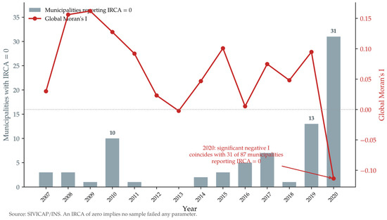
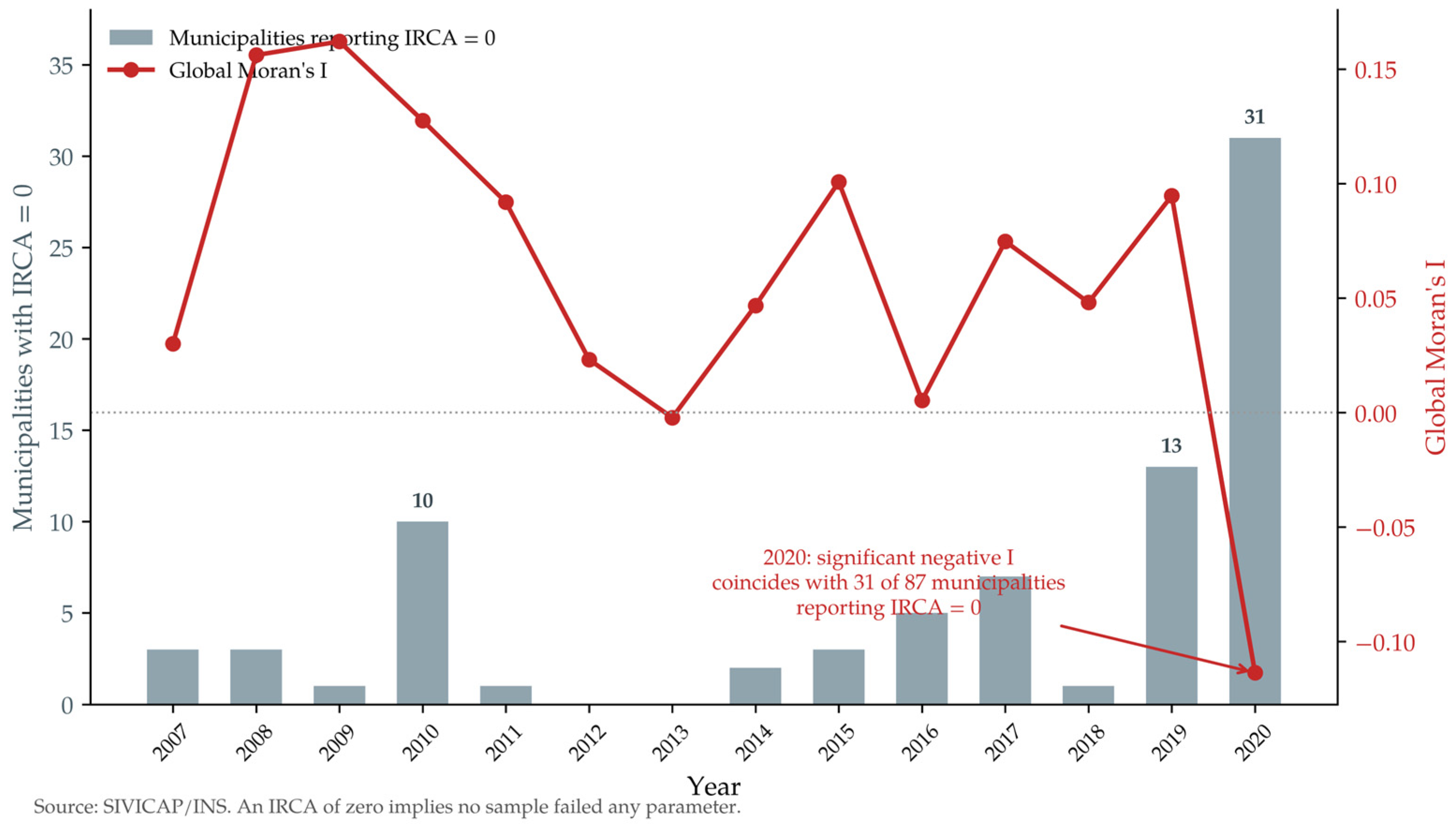
What did change abruptly was the composition of the report: municipalities with an IRCA of exactly zero rose from 1 in 2018 to 13 in 2019 and to 31 in 2020, that is, from 1% to 36% of the department in two years. A value of zero implies that no sample taken failed any parameter; its sudden multiplication is more consistent with a reduction in the number of samples taken than with a simultaneous sanitary improvement across a third of the municipalities. At the same time, very high values persisted in other territories (El Playón 80.0; Jordán 63.6; Charta 51.0; Sucre 49.5). The coexistence of a large block of zeros with scattered extreme values is the configuration that generates negative autocorrelation, and it is reflected in the −0.274 correlation between each municipality’s standardized value and that of its neighborhood.

The contrast with 2019 clarifies that 2020 is a distinct anomaly rather than the tail of a gradual trend. The correlation between each municipality’s standardized IRCA and the mean of its neighbors was 0.113 in 2018 (1% of municipalities reporting zero) and 0.201 in 2019 (15% reporting zero), remaining positive in both years; only in 2020, when 36% of municipalities reported zero, does this correlation invert to −0.274. The intermediate rise in zero-reporting observed in 2019 was therefore not sufficient to disrupt the underlying positive spatial structure, whereas the substantially higher proportion reached in 2020 was. Figure 6 shows the parallel evolution of zero-reporting municipalities and global Moran’s I.

Figure 6. The 2020 anomaly: number of municipalities reporting an IRCA of zero (bars) and global Moran’s I (line), 2007–2020. The dotted horizontal line marks zero on the Moran’s I axis.

4. Discussion

4.1. The Dissolution of Spatial Structure and What Can Be Inferred from It

Between 2007 and 2013, municipal water risk exhibited detectable spatial dependence (I = 0.113; p = 0.036), sustained under three of the five neighborhood specifications tested. Between 2014 and 2020, dependence ceased to be detectable under any of them. The share of IRCA variance attributable to the neighborhood fell from 5.0% to 1.0%.

What the data support is that the spatial structure was distinguishable from randomness in the first period and is not in the second. What cannot be stated, and therefore is not stated, is that the two coefficients differ from each other in a statistically significant way, given that the units are not independent between periods.

The decisive piece is not the comparison of the two indices but the analysis of the change. Applying the statistic to the change in IRCA between periods, no clustering is detected (I = 0.044; p = 0.198). If the improvement had spread across contiguous territories, through diffusion of practices among neighboring providers, subregional programs, or spillover effects from better-performing municipalities, the change should have shown spatial structure. It does not.

This result allows one mechanism to be ruled out and another to remain plausible. It rules out territorial diffusion as the main channel of improvement. It leaves standing the possibility that the reduction in risk responded to conditions reaching the entire department regardless of each municipality’s location. The literature on administrative surveillance indicators offers a direct precedent [25], suggesting that the loss of spatial structure in indicators of this kind is a recognizable phenomenon.

Detectability should not be confused with importance. Even in the period when spatial dependence was statistically detectable, the squared correlation between the indicator and its spatial lag ($R_{spatial}^2$, Section 2.4) was 5.0%. The finding is not that geography determined water risk, but that the geographic component, always a minority share, ceased to be distinguishable from randomness.

4.2. An Asymmetry Between Low and High Risk

Eight municipalities maintain statistically significant low-risk cluster status after controlling the false discovery rate across 87 simultaneous contrasts; none maintains the opposite condition. The asymmetry recurs across every available magnitude: 94 municipality-years versus 24; 36 municipalities versus 13; nine years of maximum recurrence versus four. The same asymmetry appears in physical units: the ten lowest-risk municipalities lie, in both periods, at a mean distance of approximately 60 km from one another, below the departmental average of 82.1 km, while the highest-risk municipalities moved from 70.6 km to 90.2 km.

The two conditions have a different nature. Low risk behaves as a property of the territory: it is located within a defined corridor, persists there over the years, and affects contiguous municipalities simultaneously. High risk behaves as a property of the unit: it appears and disappears, rotates among different municipalities, and does not form a corridor.

That difference is consistent with distinct generating processes. The conditions that sustain low risk over time, that is, installed technical capacity, consolidated providers, accessibility for technical assistance and input supply, are structural, change slowly, and are shared among nearby municipalities, thereby producing stable aggregation. The conditions that produce episodes of elevated risk in small providers are operational in nature, are resolved or reappear over short horizons, and have no reason to coincide in time among neighboring municipalities. The literature on the sustainability of rural water systems extensively documents this second type of fragility [27], and the spatial pattern observed is what would be expected if such failures occurred independently across units.

The asymmetry admits a competing, methodologically grounded reading. Thirty-two of the 87 municipalities (37%) border another department, and their neighborhoods are truncated: their actual neighbors in Boyacá, Norte de Santander, Cesar, Bolívar, or Antioquia are not part of the analysis. These municipalities have an average of 4.50 neighbors versus 5.64 for interior municipalities, which reduces the information available for their local statistics. The relevant fact is that four of the eight municipalities with the greatest recurrence of high risk lie on that border, while none of the eight significant coldspots does. One could therefore argue that hotspots fail to reach significant persistence because they are systematically measured with less precision.

The objection is pertinent and cannot be fully dismissed, but it does not explain the result. When the comparison is restricted to interior municipalities, where the neighborhood is complete, the asymmetry holds: the maximum recurrence among interior coldspots is nine years, while among interior hotspots it does not exceed three. Truncated neighborhoods likely lead to an underestimate of the number of hotspots, but the difference in magnitude between the two groups persists within the subset unaffected by the problem.

The interior-only counts underlying this comparison are reported numerically in Table 11.

Table 11. Persistence counts restricted to interior (non-border) municipalities.

Municipality	Years as Cluster	Years with Report	Status
Low-Risk Clusters (Interior)
Páramo	9	14	Yes (FDR)
San Gil	8	14	Yes (FDR)
Floridablanca	7	13	Yes (FDR)
Cabrera	6	14	No
Piedecuesta	5	12	No
Confines	5	14	No
Valle de San José	5	14	No
Palmas del Socorro	4	14	No
High-risk clusters (interior)
El Guacamayo	3	14	No
La Paz	3	14	No
Contratación	2	14	No
Jesús María	2	14	No

Note: Interior municipalities: those not bordering another department (n = 55 of 87).

4.3. Implications for Territorial Targeting

If low risk aggregates territorially and high risk does not, then the appropriate unit of intervention differs depending on the objective pursued.

In the corridor where low risk persists, the conditions that sustain it are shared among contiguous municipalities. Zonal instruments, shared laboratory networks, joint operator training, pooled procurement of inputs, and associative schemes among providers act on these shared conditions and take advantage of the documented physical proximity. Aggregation is not a design assumption: it is a measured fact.

In territories where elevated risk recurs without forming a corridor, a zonal instrument applied over an administratively defined area is highly likely to miss its target, for two reasons. First, the municipalities that register high risk in one year are not necessarily the same ones that register it three years later, so targeting based on a single period’s diagnosis arrives late. Second, the absence of clustering means that high-risk municipalities do not share a neighborhood: intervening in a zone would mean covering, for the most part, municipalities that do not need it, while omitting those that do, located at a mean distance of more than 90 km from one another.

The results support a dual targeting logic: territorial-scale instruments where demonstrated aggregation exists, and provider-level instruments where it does not. The absence of clustering in the change in IRCA reinforces this conclusion, indicating that an intervention concentrated in one municipality should not be expected to benefit its neighbors through diffusion.

The scope of these implications should be clarified. The article identifies where each targeting logic should apply, not what should be done in each case. Determining the specific instruments and their financing mechanisms lies beyond the scope of an exploratory spatial data analysis.

4.4. Spatial Diagnostics as a Surveillance Consistency Check

The year 2020 shows significant negative spatial autocorrelation (I = −0.114; p = 0.040), the only such case in the series, coinciding with an increase in municipalities reporting an IRCA of zero to 31 of 87.

A pattern of this kind is difficult to reconcile with actual changes in water quality, which do not reverse from one year to the next among territories that share watersheds and providers. What changed abruptly was the composition of the report. The sudden multiplication of null values is more consistent with a reduction in the number of samples taken than with a simultaneous sanitary improvement across a third of the department’s municipalities, in the year of the COVID-19 health emergency; this interpretation is inferential, since municipality-level sample counts are not available to the authors, and direct verification against SIVICAP’s internal sampling records would be required to confirm the mechanism.

Autocorrelation statistics are normally used to describe territorial patterns; here they function as a consistency check on the data that feed them. A sign change in Moran’s index, without a corresponding change in the mean level of the indicator, signals that the structure of reporting has been altered and that data integrity should be verified before interpretation. Applied routinely to the SIVICAP series, this check carries negligible computational cost and would allow years and territories requiring review to be identified.

4.5. Limitations

The study is descriptive. It documents the spatial structure of risk and its evolution, but does not identify causal mechanisms. Interpretations regarding the processes that would generate each pattern are consistent with the results but are not derived from them.

The IRCA is reported aggregated at the municipal level, which prevents observing internal heterogeneity between urban seats and scattered rural areas. In a department where 24% of the population lives outside municipal seats, this aggregation may conceal substantial divergences within a single unit. This is a manifestation of the modifiable areal unit problem.

The contiguity matrix assigns equal weight to all neighbors regardless of size, equating units whose population ranges from 1457 to 601,668 inhabitants and whose area ranges from 25 to 3179 km². Five alternative neighborhood specifications were tested, but none corrects for the heterogeneous content of the administrative unit.

More fundamentally, administrative contiguity approximates shared institutional context (overlapping providers, joint participation in the departmental water plan, comparable logistics for technical assistance) rather than hydrological connectivity per se, since georeferenced data on shared watersheds, raw-water intake points, and provider service areas are not available at the municipal level for the full study period. The present results should therefore be read as evidence of administrative and institutional proximity effects, not as confirmation of a specific hydrological transmission mechanism.

The detected structure is local, not subregional (Section 2.3 and Section 3.2).

As noted in Section 3.4, no individual cluster on the period maps survives the false discovery rate correction, even though the aggregate count of detected clusters exceeds chance expectations.

The persistence contrast assumes independence across the fourteen annual cross-sections. Under a conservative adjustment, the number of significant coldspots falls from eight to three and the number of hotspots remains at zero. The central conclusion holds, but the exact number of municipalities identified depends on the treatment adopted.

This effective-sample-size adjustment is a standard approximation (Bartlett’s correction) rather than a fully formal block-permutation or moving-block bootstrap procedure that would explicitly resample contiguous year-blocks to preserve the temporal dependence structure; implementing such a procedure across 87 municipalities and 14 years is identified here as a direction for future methodological work.

As shown in Section 4.2 and Table 11, the 37% of municipalities with truncated border neighborhoods likely lead to an underestimate of high-risk clusters at the periphery, though the central asymmetry holds within the unaffected interior subset.

The analysis depends on the completeness of SIVICAP, whose annual coverage ranged between 82 and 87 municipalities. Municipality-years without a report were treated as missing without imputation, which preserves data integrity but reduces power in years with lower coverage.

5. Conclusions

This article examined the spatial structure of drinking-water quality risk in the 87 municipalities of Santander between 2007 and 2020, based on 1202 municipality-year observations from the national surveillance system.

Municipal water risk exhibited positive, statistically detectable spatial autocorrelation during 2007–2013 (I = 0.113; p = 0.036), sustained under three of the five neighborhood specifications tested, and ceased to be detectable during 2014–2020 (I = 0.046; p = 0.183). The share of IRCA variance attributable to the neighborhood fell from 5.0% to 1.0%. These results support the claim that the geographic structure of risk ceased to be distinguishable from randomness, but do not warrant the claim that the two coefficients differ from each other in a statistically significant way.

The reduction in risk did not spread geographically. Applied to the change in IRCA between periods, Moran’s index detects no clustering (I = 0.044; p = 0.198). This result rules out diffusion across contiguous territories as the main channel of improvement. It should be noted that a nonsignificant result does not demonstrate the absence of clustering.

Eight municipalities maintain statistically significant low-risk cluster status after correcting for the false discovery rate, led by Páramo, significant in 9 of 14 years, San Gil in 8, and Floridablanca in 7, while no high-risk cluster reaches that threshold. The asymmetry recurs across every available magnitude: 94 municipality-years versus 24, 36 municipalities versus 13, and nine years of maximum recurrence versus four. Under a conservative adjustment for temporal dependence, the number of significant coldspots falls from eight to three and the number of hotspots remains at zero. The same asymmetry is verified in physical units: the ten lowest-risk municipalities lie at a mean distance of approximately 60 km in both periods, below the departmental average of 82.1 km, while the highest-risk municipalities moved from 70.6 km to 90.2 km. In substantive terms, low risk behaves as a property of the territory and high risk as a property of the unit.

No cluster identified on the period maps individually survives multiple-testing correction, even though the total number detected far exceeds what would be expected by chance (17 versus 4.35 expected; p = 1.3 × 10⁻⁶). Local structure exists in the territory, and the evidence from a single map is not enough to determine with confidence which municipalities constitute it. This finding motivated the design of the persistence contrast and constitutes a methodological warning applicable to other uses of local indicators on administrative units.

The year 2020 showed significant negative autocorrelation, coinciding with an increase in municipalities reporting an IRCA of zero from 1 in 2018 to 31 in 2020. The departmental mean remained stable and coverage was the highest in the series, pointing the explanation toward a disruption in sampling intensity. A practical application follows from this: spatial autocorrelation statistics can serve as a consistency check on surveillance data.

Where demonstrated aggregation exists, zonal-scale instruments act on conditions genuinely shared among nearby municipalities. Where elevated risk recurs without forming a corridor, zonal targeting would cover mostly units that do not require it. The article identifies where each targeting logic should apply, not which specific instrument corresponds to each case.

Three extensions follow from the limitations noted: incorporating weights matrices built on hydrological connectivity rather than administrative contiguity; disaggregating the indicator within municipalities where reporting permits it; and extending the series beyond 2020. In addition, applying the persistence contrast proposed here to other departments would help determine whether the documented asymmetry is a general feature of the sector or a peculiarity of the case analyzed.

References

- Wolf, J.; Johnston, R.B.; Ambelu, A.; Arnold, B.F.; Bain, R.; Brauer, M.; Brown, J.; Caruso, B.A.; Clasen, T.; Colford, J.M., Jr.; et al. Burden of disease attributable to unsafe drinking water, sanitation, and hygiene in domestic settings: A global analysis for selected adverse health outcomes. Lancet 2023, 401, 2060–2071. [Google Scholar] [CrossRef] [Scilit]
- UNICEF; WHO. Progress on Household Drinking Water, Sanitation and Hygiene 2000–2022: Special Focus on Gender; UNICEF: New York, NY, USA; WHO: Geneva, Switzerland, 2023. [Google Scholar]
- World Health Organization. Guidelines for Drinking-Water Quality, 4th ed.; Incorporating the first addendum; WHO: Geneva, Switzerland, 2017. [Google Scholar]
- UN-Water. SDG 6 Data Portal—Country Profile: Colombia; United Nations: Geneva, Switzerland, 2024; Available online: https://www.sdg6data.org/es/country-or-area/Colombia (accessed on 30 July 2026).
- Ministerio de la Protección Social. Decreto 1575 de 2007; Diario Oficial 46.623: Bogotá, Colombia, 2007. [Google Scholar]
- Ministerio de la Protección Social; Ministerio de Ambiente, Vivienda y Desarrollo Territorial. Resolución 2115 de 2007; Ministerio de la Protección Social: Bogotá, Colombia, 2007. [Google Scholar]
- Instituto Nacional de Salud. SIVICAP: Datos Municipales de IRCA 2007–2020; INS: Bogotá, Colombia, 2021. [Google Scholar]
- Ministerio de Ambiente, Vivienda y Desarrollo Territorial. Política Nacional para la Gestión Integral del Recurso Hídrico; MAVDT: Bogotá, Colombia, 2010. [Google Scholar]
- Henao-Rodríguez, C.; Lis-Gutiérrez, J.-P.; Vidal, D.G. Water injustice in Colombia: Perceptions and realities of water quality examined through advanced machine learning. PLoS ONE 2025, 20, e0332274. [Google Scholar] [CrossRef] [Scilit]
- Castillo-Castillo, A.; El-Khattabi, A.R.; Fernandez, J. A spatio-temporal analysis of water investment allocation in Colombia and its impacts on drinking water quality. Environ. Res. Lett. 2025, 20, 034025. [Google Scholar] [CrossRef] [Scilit]
- Peña-Guzmán, C.A.; Soto, L.; Diaz, A. A proposal for redesigning the water quality network of the Tunjuelo River in Bogotá, Colombia through a spatio-temporal analysis. Resources 2019, 8, 64. [Google Scholar] [CrossRef] [Scilit]
- Matta-Ortíz, A.F.; Güiza-Valdes, I.A.; Trujillo-González, J.M.; Rojas-Peña, J.I.; Torres-Mora, M.A.; García-Navarro, F.J.; Jiménez-Ballesta, R. Assessing rainwater quality and harvesting potential: A spatial analysis in a medium-sized city of Colombia. Water 2024, 16, 3411. [Google Scholar] [CrossRef] [Scilit]
- Tobler, W.R. A computer movie simulating urban growth in the Detroit region. Econ. Geogr. 1970, 46, 234–240. [Google Scholar] [CrossRef] [Scilit] [PubMed]
- Demoze, L.; Adane, K.C.; Azanaw, J.; Akalewold, E.; Enawugaw, T.; Tigabie, M.; Tesfaye, A.H.; Yitageasu, G. Spatial analysis of unimproved drinking water source in East Africa: Using Demographic and Health Survey data from 2012–2023. PLoS ONE 2025, 20, e0318189. [Google Scholar] [CrossRef] [Scilit]
- Yitageasu, G.; Alemu, E.A.; Gebrehana, A.K.; Asnake, A.A.; Demoze, L. Geospatial analysis and prevalence estimation of household drinking water treatment in sub-Saharan African countries: Insights from recent Demographic and Health Surveys. J. Egypt. Public Health Assoc. 2026, 101, 10. [Google Scholar] [CrossRef] [Scilit]
- Chaudhari, U.; Kumari, D.; Mittal, S.; Sahoo, P.K. GIS-based spatial autocorrelation and multivariate statistics for understanding groundwater uranium contamination and associated health risk in semiarid region of Punjab, India. Water 2025, 17, 2064. [Google Scholar] [CrossRef] [Scilit]
- Departamento Administrativo Nacional de Estadística. Marco Geoestadístico Nacional 2018; DANE: Bogotá, Colombia, 2018. [Google Scholar]
- Departamento Administrativo Nacional de Estadística. Proyecciones de Población Municipal 2005–2042, Base CNPV 2018; DANE: Bogotá, Colombia, 2020. [Google Scholar]
- Asamblea Departamental de Santander. Ordenanza 009 de 2019; por la Cual se Crean las Provincias Administrativas y de Planificación; Asamblea Departamental de Santander: Bucaramanga, Colombia, 2019. [Google Scholar]
- Moran, P.A.P. Notes on continuous stochastic phenomena. Biometrika 1950, 37, 17–23. [Google Scholar] [CrossRef] [Scilit]
- Anselin, L. Local indicators of spatial association—LISA. Geogr. Anal. 1995, 27, 93–115. [Google Scholar] [CrossRef] [Scilit]
- Ord, J.K.; Getis, A. Local spatial autocorrelation statistics: Distributional issues and an application. Geogr. Anal. 1995, 27, 286–306. [Google Scholar] [CrossRef] [Scilit]
- Benjamini, Y.; Hochberg, Y. Controlling the false discovery rate: A practical and powerful approach to multiple testing. J. R. Stat. Soc. Ser. B (Methodol.) 1995, 57, 289–300. [Google Scholar] [CrossRef] [Scilit]
- Rey, S.J.; Anselin, L. PySAL: A Python library of spatial analytical methods. Rev. Reg. Stud. 2007, 37, 5–27. [Google Scholar] [CrossRef] [Scilit]
- Ngmenbelle, D.; Amoa-Saah, B.; Nimirkpen, S.; Akesem, M.A.; Idan, J.S.; Mohammed, A. Spatiotemporal hotspot analysis of tuberculosis lost to follow-up cases in Ghana: A district-level study from 2019–2023. PLoS ONE 2025, 20, e0326444. [Google Scholar] [CrossRef] [Scilit]
- Machado, A.; Oliveira, M.; Fernandes, C. A physiologically-based model for simulation of color vision deficiency. IEEE Trans. Vis. Comput. Graph. 2009, 15, 1291–1298. [Google Scholar] [CrossRef] [Scilit]
- Lockwood, H.; Smits, S. Supporting Rural Water Supply: Moving Towards a Service Delivery Approach; Practical Action Publishing: Rugby, UK, 2011; ISBN 978-1-85339-729-5. [Google Scholar]
Disclaimer/Publisher’s Note: The statements, opinions and data contained in all publications are solely those of the individual author(s) and contributor(s) and not of MDPI and/or the editor(s). MDPI and/or the editor(s) disclaim responsibility for any injury to people or property resulting from any ideas, methods, instructions or products referred to in the content. |
© 2026 by the authors. Licensee MDPI, Basel, Switzerland. This article is an open access article distributed under the terms and conditions of the Creative Commons Attribution (CC BY) license.