Heterogeneity-Aware Multi-Step Chlorophyll-a Forecasting for Marine Water Quality Monitoring Using a Multi-Scale Spatio-Temporal Mixture-of-Experts Network

Abstract

Chlorophyll-a concentration (Chl-a) is a key indicator of marine water quality, phytoplankton biomass, and aquatic ecosystem status. Multi-step forecasting is challenging because Chl-a dynamics exhibit regional heterogeneity, multi-scale variability, and complex spatial dependence. Existing models often optimize domain-averaged errors, which can mask unstable node-level predictions at high-variability nodes. We propose MS-STMoE, a heterogeneity-aware multi-scale spatio-temporal mixture-of-experts framework. It uses a Haversine-distance-based K-nearest-neighbor graph, gated multi-scale temporal convolutions with seasonal encoding to model short-term and periodic variations, and node-level sparse top-k routing that assigns differentiated expert pathways to nodes with distinct dynamics based on recent-state, temporal-mean, temporal-change, and node-prior features. Using 30-day histories to forecast the next 15 days, experiments on 300 Bohai Sea and 265 South China Sea nodes show that MS-STMoE achieves the lowest average MAE and RMSE among six recent spatio-temporal baselines. Compared with the best baseline, MAE and RMSE decrease by 5.6% and 2.7%, respectively, in the Bohai Sea, and by 11.0% and 5.0%, respectively, in the South China Sea. Step-wise and node-wise analyses indicate improved medium-to-late-horizon accuracy and modest, region-dependent reductions in high-error node tails, supporting more reliable region-aware short- to medium-term water quality monitoring.

1. Introduction

Chlorophyll-a concentration (Chl-a) is a key indicator of marine water quality, phytoplankton biomass, primary productivity, and aquatic ecosystem status. Its spatio-temporal variability provides important information for harmful algal bloom monitoring, eutrophication assessment, fishery resource evaluation, coastal ecosystem protection, and marine environmental management [1]. With the development of satellite remote sensing, ocean color observations, and marine monitoring technologies, long-term and large-scale Chl-a datasets have become increasingly available, providing a valuable basis for data-driven water quality forecasting and ecological early-warning applications [2]. Reliable short- to medium-term Chl-a forecasting can support timely identification of abnormal phytoplankton variations and marine water quality management.

Reliable Chl-a forecasting remains challenging because Chl-a dynamics are jointly affected by seasonal variability, solar radiation, nutrient availability, terrestrial inputs, ocean current transport, water mixing, and local hydrodynamic processes [3]. These factors can lead to strong nonlinearity, nonstationary temporal variations, complex spatial dependence, and pronounced regional heterogeneity. Coastal waters are often affected by river discharge, anthropogenic inputs, and nearshore mixing processes; semi-enclosed seas may exhibit stronger retention effects and seasonal accumulation; and offshore regions are more strongly influenced by large-scale circulation, fronts, and climate-related processes [4]. Therefore, simultaneously modeling multi-scale temporal dependencies, spatial correlations, and region-specific variation patterns remains an important problem in marine Chl-a forecasting [5].

Existing Chl-a forecasting studies have evolved from traditional statistical and machine learning methods to deep learning models. Traditional approaches, such as autoregressive models, support vector regression, and random forests, can describe certain temporal variations in Chl-a concentration, but they often rely on linear assumptions, handcrafted features, or fixed model structures [6,7]. Deep learning methods, including convolutional neural networks (CNNs), long short-term memory networks (LSTMs), ConvLSTM, Transformer-based models, and graph neural networks (GNNs), have been increasingly used for Chl-a forecasting and marine environmental prediction [8,9,10,11,12]. Although these models can improve nonlinear spatio-temporal representation ability, many of them mainly optimize global average errors and pay limited attention to spatially uneven prediction behavior among marine regions, which may lead to unstable performance in coastal waters, high-variability areas, or locations with abrupt Chl-a changes [13].

For marine water quality monitoring, spatially heterogeneous prediction behavior is particularly important. A forecasting model that performs well on average may still produce large errors at ecologically sensitive or high-Chl-a locations. Different marine nodes may correspond to different ecological and hydrodynamic regimes [14]. For example, Chl-a variations in coastal or semi-enclosed waters may be related to local nutrient enrichment, terrestrial inputs, and water retention, whereas offshore Chl-a variations may be more affected by large-scale circulation and seasonal oceanographic processes [15]. Since Chl-a variations also occur at multiple temporal scales, a single shared forecasting structure may be insufficient to represent diverse spatio-temporal patterns across heterogeneous marine environments.

Mixture-of-Experts (MoE) models provide a flexible mechanism for modeling heterogeneous data patterns by dynamically routing input representations to different expert subnetworks through a gating network [16]. In spatio-temporal forecasting, sparse expert routing allows different spatial units and temporal states to use different forecasting pathways. Previous studies have shown that expert-based routing can improve heterogeneous spatio-temporal forecasting [17]. This idea is relevant to marine Chl-a forecasting because different spatial nodes may exhibit distinct and time-varying dynamics. Therefore, sparse expert routing may be suitable for adapting forecasting models to region-specific Chl-a variation patterns under heterogeneous marine water quality conditions.

Based on this motivation, this study develops MS-STMoE, a multi-scale spatio-temporal mixture-of-experts framework for heterogeneity-aware multi-step Chl-a forecasting in marine water quality monitoring. The proposed framework constructs a geographical distance graph from observation nodes to describe spatial adjacency among marine locations, uses graph convolution to extract spatial dependencies, and applies multi-scale temporal convolution to capture both short-term fluctuations and longer temporal evolution. A sparse MoE module further routes node-level spatio-temporal representations to expert subnetworks, supporting differentiated modeling of diverse marine variation patterns. In addition to overall forecasting accuracy, this study evaluates step-wise prediction errors and node-level spatial error distributions to characterize model behavior across heterogeneous marine regions.

The main contributions of this study are summarized as follows:

• To address the limitation that globally shared predictors may overlook distinct node-level Chl-a dynamics, we develop MS-STMoE, a heterogeneity-aware forecasting framework with node-level sparse expert routing. The routing mechanism assigns differentiated expert pathways to nodes with distinct dynamic patterns rather than enforcing a uniform prediction pathway across the study region.
• To provide the routing mechanism with informative representations across spatial locations and temporal scales, the framework integrates a Haversine-distance-based geographical graph, gated multi-scale temporal convolutions, and seasonal encoding. Recent-state, temporal-mean, temporal-change, and node-prior features are jointly used to distinguish node-specific forecasting requirements.
• Experiments across the semi-enclosed Bohai Sea and the open South China Sea demonstrate consistent improvements over six recent spatio-temporal baselines. Step-wise and node-wise analyses show that the complete framework achieves its strongest gains at medium-to-late forecast horizons and reduces high-error node tails relative to STAEformer, while the incremental contribution of sparse routing remains modest and region-dependent.

2. Related Work

2.1. Chl-a Forecasting for Marine Water Quality Monitoring

Chlorophyll-a concentration (Chl-a) forecasting is an important task in marine water quality monitoring, harmful algal bloom early warning, and aquatic ecosystem assessment. Since Chl-a reflects phytoplankton biomass and primary productivity, reliable prediction of its temporal evolution can provide useful information for identifying abnormal ecological changes and supporting coastal environmental management. Early Chl-a forecasting studies mainly relied on statistical models and traditional machine learning methods. Autoregressive models have been used to describe temporal variations in water quality variables, while support vector regression, random forests, and other machine learning methods have been applied to Chl-a prediction and bloom-related assessment [6,18,19]. These methods can be effective for specific regions or short-term forecasting tasks, but their performance may be limited by handcrafted features, fixed parameter structures, or insufficient nonlinear representation ability.

With the increasing availability of satellite observations and in situ monitoring data, deep learning methods have been introduced to improve Chl-a forecasting. LSTM-based models have been used to capture temporal dependencies in water quality sequences [20], while CNN- or ConvLSTM-based structures can extract spatial and temporal features from remote sensing observations [21]. These developments have strengthened nonlinear temporal representation, but jointly capturing short-term fluctuations, longer periodic variations, and spatial context remains challenging. This motivates spatio-temporal modeling approaches that make more explicit use of the structure and characteristics of marine observations.

2.2. Remote Sensing and Spatio-Temporal Deep Learning for Marine Environmental Prediction

Ocean color remote sensing provides an important data source for large-scale Chl-a monitoring because it enables repeated and synoptic observation of phytoplankton variability over broad marine regions [22,23]. Compared with sparse field observations, satellite-derived Chl-a products offer wider spatial coverage and longer temporal records, making them suitable for data-driven marine water quality forecasting [22,24]. However, remote sensing-based Chl-a data can be affected by cloud contamination, sun glint, atmospheric correction uncertainty, missing observations, and complex coastal optical conditions [23,24]. These factors increase the difficulty of constructing reliable forecasting models, especially in coastal waters and semi-enclosed seas where Chl-a variability can be highly irregular [23].

Recent studies have used remote sensing observations together with spatio-temporal deep learning models to predict Chl-a and related marine environmental variables. Yao et al. [8] predicted sea surface Chl-a concentrations using deep learning and time-series remote sensing data. Sun et al. [9] integrated Fourier analysis and Transformer networks to enhance Chl-a forecasting in coastal waters. Zhou et al. [10] developed a spatio-temporal fusion Transformer model for large-area Chl-a prediction using satellite time series. Similar spatio-temporal modeling ideas have also been applied to sea surface temperature and other marine variables [25,26]. These studies demonstrate the potential of remote sensing and deep learning for marine environmental prediction. However, many of these approaches are developed for regular satellite grids, whereas selected observation nodes or spatially incomplete marine data may require more flexible representations of spatial relationships.

Graph neural networks provide a flexible way to model irregular spatial relationships by representing observation locations as graph nodes. This is useful for marine observation points and remote sensing sampling locations that cannot always be represented as regular grids. Graph-based neural representations have been explored for nonuniform spatial data [27], while related spatio-temporal models have been developed for marine-variable forecasting [28]. For Chl-a prediction, graph-based and hybrid deep learning models have also been used to model spatial interactions among marine locations [11,12]. These studies indicate that graph-based models can be suitable for irregular marine nodes and complex spatial dependence. However, graph-based spatial connectivity alone does not ensure adaptation to node-specific dynamics, because many existing spatio-temporal models still apply a largely shared prediction structure across locations. Thus, the remaining challenge is not only how nodes are spatially connected, but also whether distinct nodes can follow different forecasting pathways.

2.3. Spatio-Temporal Heterogeneity in Chl-a Dynamics

Chl-a concentration exhibits significant regional heterogeneity due to differences in nutrient supply, light availability, hydrodynamic conditions, terrestrial inputs, and biological processes. Large-scale studies have reported changes in ocean greenness and phytoplankton bloom patterns, indicating that Chl-a variations are closely related to regional environmental conditions and climate-related processes [1,29]. In coastal and semi-enclosed waters, Chl-a dynamics can be strongly affected by river discharge, anthropogenic nutrient inputs, retention effects, and seasonal accumulation. Shafeeque et al. [30] showed that semi-enclosed bays can present strong regional Chl-a modulation, while Kim et al. [14] reported that coastal and offshore waters may exhibit different seasonal Chl-a patterns. These broad regional contrasts emerge from interacting processes operating across multiple spatial and temporal scales, and local studies provide further evidence of how individual drivers generate distinct Chl-a dynamics at specific marine locations.

Several studies have further examined the mechanisms behind local Chl-a variability. Xu et al. [31] showed that phytoplankton blooms near the Changjiang River Estuary are jointly influenced by river discharge, monsoon forcing, and hydrodynamic processes. Zhu et al. [32] found that mesoscale eddies can modify offshore Chl-a distributions through upwelling or the transport of nearshore high-Chl-a water. Li et al. [33] also emphasized the influence of offshore circulation, fronts, and eddies on primary production and Chl-a distributions. Collectively, these processes can produce node-specific concentration ranges, variability amplitudes, rates of change, seasonal patterns, and levels of predictability. These findings suggest that different marine locations may have different forecasting difficulties. A model that only minimizes global average errors may fit dominant or stable regions well but still perform poorly in coastal, high-variability, or locally abnormal regions. Therefore, Chl-a forecasting studies should not only consider overall accuracy but also spatial error distributions and local prediction behavior. Beyond evaluation, this heterogeneity also imposes explicit constraints on model design. Spatial representations should preserve geographically meaningful relationships among irregular marine nodes, temporal representations should capture both short-term fluctuations and recurring or seasonal variations, and the forecasting mechanism should permit node-level adaptation rather than rely exclusively on a single globally shared prediction pathway. These requirements motivate geographical graph modeling, multi-scale temporal representation learning, and adaptive node-level routing in the subsequent methodology.

2.4. Mixture-of-Experts for Heterogeneous Forecasting

Mixture-of-Experts (MoE) models dynamically assign input representations to different expert subnetworks through a gating network, providing a flexible mechanism for modeling heterogeneous and nonstationary data patterns. Recent studies have applied MoE to time series forecasting to improve the representation of diverse temporal dynamics [16,34,35]. In spatio-temporal forecasting, MoE can be useful because different spatial units may require different forecasting pathways. Li et al. [17] showed that sparse expert routing can improve heterogeneous spatio-temporal forecasting by assigning different spatial units to suitable expert pathways. Marine Chl-a forecasting faces a related modeling challenge because different spatial nodes may exhibit distinct and time-varying dynamics under heterogeneous ecological and hydrodynamic conditions. This makes sparse expert routing relevant for heterogeneity-aware Chl-a forecasting, although the learned experts should be interpreted as data-driven representations rather than fixed physical regimes. Accordingly, sparse expert routing provides a direct mechanism for satisfying the node-adaptation requirement identified above while retaining shared spatio-temporal representations. This motivates integrating geographical graph modeling and multi-scale temporal features with node-level sparse expert routing in the proposed heterogeneity-aware Chl-a forecasting framework.

3. Proposed Method

3.1. Problem Definition and Notations

In this study, marine chlorophyll-a concentration (Chl-a) multi-step forecasting is formulated as a graph-based multi-node spatio-temporal sequence forecasting problem for marine water quality monitoring. Let $V=\{v_1,v_2,\dots ,v_N\}$ denote a set of N marine observation nodes, where each node corresponds to a spatial location with latitude and longitude information. The spatial relationships among nodes are represented by a graph $G=(V,\mathcal{E},A)$, where $\mathcal{E}$ is the edge set and $A\in {\mathbb{R}}^{N\times N}$ is the adjacency matrix.

Let $c_t^i$ denote the original Chl-a concentration at node $v_i$ and time step t, and let $x_t^i$ denote the corresponding transformed and standardized value. Given historical input features over the past T time steps, the input tensor is denoted by

$${\mathbf{Z}}_{t-T+1:t}=[{\mathbf{Z}}_{t-T+1},{\mathbf{Z}}_{t-T+2},\dots ,{\mathbf{Z}}_t]\in {\mathbb{R}}^{T\times N\times C},$$

(1)

where ${\mathbf{Z}}_t\in {\mathbb{R}}^{N\times C}$ denotes the node-level input features at time step t, and C is the input feature dimension. In this study, the input features consist of standardized historical Chl-a values and seasonal encodings. The forecasting target is the future standardized Chl-a sequence over all marine nodes:

$${\widehat{\mathbf{X}}}_{t+1:t+H}=f_{\theta }({\mathbf{Z}}_{t-T+1:t},G),{\widehat{\mathbf{X}}}_{t+1:t+H}\in {\mathbb{R}}^{H\times N},$$

(2)

where H denotes the forecasting horizon and $\theta$ denotes the learnable parameters. The corresponding ground-truth sequence is denoted as ${\mathbf{X}}_{t+1:t+H}\in {\mathbb{R}}^{H\times N}$. Model training and prediction are performed on the transformed and standardized Chl-a scale, while evaluation metrics are calculated on the original Chl-a concentration scale after inverse standardization and inverse logarithmic transformation.

3.2. Overview of the Proposed Framework

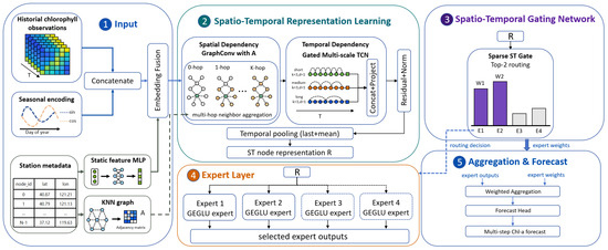
As shown in Figure 1, the proposed MS-STMoE framework consists of four main components: input representation and geographical graph construction, spatio-temporal representation learning, sparse spatio-temporal mixture-of-experts, and multi-step forecasting. Standardized historical Chl-a values are concatenated with seasonal encodings and projected into a latent representation. A geographical K-nearest-neighbor (KNN) graph is constructed from node coordinates to describe spatial adjacency among marine locations. The spatio-temporal representation module captures spatial dependencies through graph convolution and nonstationary multi-scale temporal variations through gated multi-scale temporal convolution. Based on the learned node-level spatio-temporal representations, a sparse gating network routes different marine nodes to suitable expert subnetworks. The experts are not assumed to represent fixed physical mechanisms; rather, they are designed to learn different data-driven spatio-temporal regimes under heterogeneous marine conditions. The aggregated expert outputs are then used to generate multi-step Chl-a forecasts.

3.3. Input Representation and Geographical Graph Construction

Before model training, original Chl-a values are transformed using $\log (1+c)$ to reduce the influence of extreme values and right-skewed concentration distributions. The transformed values are then standardized using the mean and standard deviation computed only from the training set:

$$x_t^i={\displaystyle \frac{\log (1+c_t^i)-{\mu }_{\mathrm{tr}}}{s_{\mathrm{tr}}}},$$

(3)

where $c_t^i$ is the original Chl-a concentration at node $v_i$ and time step t and ${\mu }_{\mathrm{tr}}$ and $s_{\mathrm{tr}}$ are the mean and standard deviation calculated from the training set. The same training-set statistics are applied to the validation and test sets to avoid information leakage. Latitude and longitude metadata are also standardized before being used as static node features.

To explicitly represent annual periodicity, day-of-year encoding is introduced:

$${\mathbf{s}}_t=\left[\sin \left({\displaystyle \frac{2\pi d_t}{P}}\right),\cos \left({\displaystyle \frac{2\pi d_t}{P}}\right)\right],$$

(4)

where $d_t$ is the day index and P denotes the annual period. For node $v_i$, the input feature is obtained by concatenating the standardized Chl-a value and seasonal encoding:

$${\mathbf{z}}_t^i=[x_t^i;{\mathbf{s}}_t].$$

(5)

Node metadata are projected into the latent space through a static feature multilayer perceptron:

$${\mathbf{m}}_i={\mathrm{MLP}}_s\left({\ell }_i\right),$$

(6)

where ${\ell }_i$ denotes the standardized latitude and longitude metadata of node $v_i$. The initial hidden representation is then computed as

$${\mathbf{H}}_{\mathrm{hid},t,i}^{\left(0\right)}={\mathbf{z}}_t^i{\mathbf{W}}_{in}+{\mathbf{e}}_i+{\mathbf{m}}_i,$$

(7)

where ${\mathbf{W}}_{in}$ is the input projection matrix, ${\mathbf{e}}_i$ is the learnable node embedding, and ${\mathbf{H}}_{\mathrm{hid}}^{\left(0\right)}\in {\mathbb{R}}^{T\times N\times D}$ denotes the initial hidden representation.

The geographical graph is constructed according to the Haversine distance between marine nodes. Geographically nearby marine locations are more likely to share similar coastal forcing, hydrodynamic conditions, and phytoplankton variability, making distance-based graph construction a reasonable baseline for representing spatial adjacency in Chl-a forecasting. For each node, its $K_g$ nearest neighbors are selected, and the initial adjacency weight is defined as

$$A_{ij}^0=\left\{\begin{array}{cc}\exp \left(-d_{ij}^2/{\sigma }_A^2\right),\hfill & v_j\in {\mathcal{N}}_{K_g}\left(v_i\right),\hfill \\ 0,\hfill & \mathrm{otherwise},\hfill \end{array}\right.$$

(8)

where $d_{ij}$ is the Haversine distance between nodes $v_i$ and $v_j$, ${\mathcal{N}}_{K_g}\left(v_i\right)$ denotes the $K_g$ nearest neighbors of $v_i$, and ${\sigma }_A$ is set as the median of all positive distances among the selected KNN edges. To avoid directional artifacts caused by the KNN procedure, the adjacency matrix is symmetrized as

$$A=\max (A^0,{\left(A^0\right)}^{\top }).$$

(9)

Self-loops are added and the adjacency matrix is symmetrically normalized:

$$\tilde{A}=D_A^{-\frac{1}{2}}(A+I)D_A^{-\frac{1}{2}},$$

(10)

where $D_A$ is the degree matrix of $A+I$.

3.4. Spatio-Temporal Representation Learning

The spatio-temporal representation learning module consists of a multi-hop graph convolution module and a gated multi-scale temporal convolution module. The spatial module captures dependencies among marine nodes, while the temporal module extracts Chl-a variation patterns over different time scales.

3.4.1. Spatial Dependency Modeling

Marine Chl-a dynamics may be affected by both local interactions and broader regional processes. Therefore, multi-hop graph convolution is adopted to capture spatial dependencies at different neighborhood ranges:

$${\mathbf{H}}_{\mathrm{sp}}^{\left(l\right)}={\displaystyle \sum _{k=0}^{K_s}}{\tilde{A}}^k{\mathbf{H}}_{\mathrm{hid}}^{(l-1)}{\mathbf{W}}_k^{\left(l\right)},$$

(11)

where $K_s$ denotes the maximum spatial hop, ${\tilde{A}}^k$ represents the k-hop graph propagation matrix, and ${\mathbf{W}}_k^{\left(l\right)}$ is the learnable transformation matrix. The term $k=0$ corresponds to self-representation. A residual connection and layer normalization are then applied:

$${\mathbf{S}}^{\left(l\right)}=\mathrm{LayerNorm}\left({\mathbf{H}}_{\mathrm{hid}}^{(l-1)}+\mathrm{GELU}\left({\mathbf{H}}_{\mathrm{sp}}^{\left(l\right)}\right)\right).$$

(12)

3.4.2. Temporal Dependency Modeling

To capture temporal dependencies at different scales, M temporal convolution branches are applied along the time dimension. Each branch uses a specific kernel size and dilation rate:

$${\mathbf{U}}_m^{\left(l\right)}={\mathrm{Conv}}_{k_m,d_m}\left({\mathbf{S}}^{\left(l\right)}\right),m=1,2,\dots ,M,$$

(13)

where $k_m$ and $d_m$ denote the kernel size and dilation rate of the m-th branch, respectively. The temporal convolutions are applied only to the historical input window, so future observations are not used when generating forecasts. The specific kernel sizes and dilation rates are treated as dataset-specific hyperparameters and are reported in the experimental settings.

Each branch adopts a gated mechanism:

$${\mathbf{T}}_m^{\left(l\right)}={\mathbf{P}}_m^{\left(l\right)}\odot \sigma \left({\mathbf{Q}}_m^{\left(l\right)}\right),[{\mathbf{P}}_m^{\left(l\right)};{\mathbf{Q}}_m^{\left(l\right)}]={\mathbf{U}}_m^{\left(l\right)}.$$

(14)

The outputs of all temporal branches are concatenated and projected back to the latent dimension:

$${\mathbf{T}}^{\left(l\right)}={\mathrm{MLP}}_t\left([{\mathbf{T}}_1^{\left(l\right)};{\mathbf{T}}_2^{\left(l\right)};\cdots ;{\mathbf{T}}_M^{\left(l\right)}]\right).$$

(15)

The output of the l-th spatio-temporal layer is obtained as

$${\mathbf{H}}_{\mathrm{hid}}^{\left(l\right)}=\mathrm{LayerNorm}\left({\mathbf{S}}^{\left(l\right)}+\mathrm{GELU}\left({\mathbf{T}}^{\left(l\right)}\right)\right).$$

(16)

After stacking L spatio-temporal layers, the recent state, temporal mean state, and temporal change state are extracted as

$${\mathbf{R}}^{\mathrm{last}}={\mathbf{H}}_{\mathrm{hid},T}^{\left(L\right)},{\mathbf{R}}^{\mathrm{mean}}={\displaystyle \frac{1}{T}}{\displaystyle \sum _{\tau =1}^T}{\mathbf{H}}_{\mathrm{hid},\tau }^{\left(L\right)},{\mathbf{R}}^{\mathrm{change}}={\mathbf{H}}_{\mathrm{hid},T}^{\left(L\right)}-{\mathbf{H}}_{\mathrm{hid},1}^{\left(L\right)}.$$

(17)

The node-level spatio-temporal representation used for forecasting is computed as

$$\mathbf{R}=\mathrm{LayerNorm}\left({\mathbf{R}}^{\mathrm{last}}+{\mathbf{R}}^{\mathrm{mean}}\right),$$

(18)

where $\mathbf{R}\in {\mathbb{R}}^{N\times D}$. The temporal change state is further used in the routing context to support expert selection under temporally varying Chl-a conditions.

3.5. Sparse Spatio-Temporal Mixture-of-Experts

Due to the regional heterogeneity of marine Chl-a dynamics, different nodes may require different transformations of their spatio-temporal representations. To provide differentiated forecasting pathways, a sparse spatio-temporal mixture-of-experts module is introduced. Here, an “expert” denotes a trainable neural subnetwork rather than a human participant or a predefined geographical group. All experts use the same GEGLU feed-forward architecture but have independently learned parameters, allowing them to represent different data-driven transformations. They are not assigned fixed physical meanings, such as coastal, semi-enclosed, or offshore regimes. The module adopts node-level and input-dependent routing, through which each marine node selects an expert combination according to its current spatio-temporal representation.

To make the routing decision aware of local temporal variation and node-specific priors, a compact routing context is constructed as

$${\mathbf{r}}_i={\mathrm{MLP}}_r\left([{\mathbf{R}}_i^{\mathrm{last}};{\mathbf{R}}_i^{\mathrm{mean}};{\mathbf{R}}_i^{\mathrm{change}};{\mathbf{p}}_i]\right),$$

(19)

where ${\mathbf{p}}_i$ denotes the node prior formed by the learnable node embedding and static coordinate representation. The routing context therefore jointly encodes the recent state, temporal-mean condition, temporal-change tendency, and node-specific prior of each marine location.

Given the representation ${\mathbf{R}}_i$ of node $v_i$, the router logits are computed as

$${\mathbf{q}}_i=\mathrm{LayerNorm}\left({\mathbf{R}}_i+{\mathbf{r}}_i\right){\mathbf{W}}_g,$$

(20)

where ${\mathbf{W}}_g\in {\mathbb{R}}^{D\times E}$ and E is the number of experts. Each component of ${\mathbf{q}}_i$ represents a learned compatibility score between node $v_i$ and one expert. Only the top $K_e$ experts are selected:

$${\mathcal{S}}_i=\mathrm{TopK}({\mathbf{q}}_i,K_e).$$

(21)

The sparse routing weight is computed by applying softmax over the selected experts:

$$g_{i,e}=\left\{\begin{array}{cc}{\displaystyle \frac{\exp \left(q_{i,e}\right)}{{\sum }_{j\in {\mathcal{S}}_i}\exp \left(q_{i,j}\right)},}\hfill & e\in {\mathcal{S}}_i,\hfill \\ 0,\hfill & e\notin {\mathcal{S}}_i.\hfill \end{array}\right.$$

(22)

For each node in each input sample, the router activates the top-$K_e$ experts with the highest routing scores, whereas all remaining experts receive zero routing weight. The normalized weights determine the relative contribution of the selected experts to the aggregated expert representation. Therefore, expert selection is based on learned node-level routing scores rather than manually specified thresholds, regional labels, or predefined node groups. Because the routing context is partly derived from the current historical input window, the same node may activate different expert combinations under different temporal conditions.

Each expert is implemented as a GEGLU feed-forward network:

$$E_e\left({\mathbf{R}}_i\right)={\mathbf{W}}_{e,2}\left[\left({\mathbf{R}}_i{\mathbf{W}}_{e,1}\right)\odot \mathrm{GELU}\left({\mathbf{R}}_i{\mathbf{W}}_{e,g}\right)\right].$$

(23)

The sparse expert aggregation is defined as

$${\overline{\mathbf{o}}}_i=\sum _{e\in {\mathcal{S}}_i}{g}_{i,e}{E}_e\left({\mathbf{R}}_i\right).$$

(24)

A residual connection with a learnable scaling coefficient is used to stabilize the MoE block:

$${\mathbf{o}}_i={\mathbf{R}}_i+{\alpha }_{\mathrm{moe}}{\overline{\mathbf{o}}}_i,$$

(25)

where ${\alpha }_{\mathrm{moe}}$ controls the contribution of the sparse expert output. The router and expert subnetworks are jointly optimized end-to-end through the training objective described in Section 3.6. The prediction loss encourages useful routing pathways, while the expert balance and router regularization terms discourage routing collapse and stabilize the routing logits. No expert labels or manual node-to-expert assignments are required.

3.6. Forecasting Output and Training Objective

The aggregated expert output is fed into a forecasting head to generate multi-step predictions on the transformed and standardized Chl-a scale:

$${\widehat{\mathbf{x}}}_i={\mathrm{MLP}}_{out}\left({\mathbf{o}}_i\right),{\widehat{\mathbf{x}}}_i\in {\mathbb{R}}^H.$$

(26)

The predictions of all nodes are stacked to form the final forecasting output:

$${\widehat{\mathbf{X}}}_{t+1:t+H}=[{\widehat{\mathbf{x}}}_1,{\widehat{\mathbf{x}}}_2,\dots ,{\widehat{\mathbf{x}}}_N]\in {\mathbb{R}}^{H\times N}.$$

(27)

The main prediction loss is defined over all training samples, future time steps, and spatial nodes using the Huber loss:

$${\mathcal{L}}_{pred}={\displaystyle \frac{1}{BHN}}{\displaystyle \sum _{b=1}^B}{\displaystyle \sum _{h=1}^H}{\displaystyle \sum _{i=1}^N}{\rho }_{\delta }\left({\widehat{x}}_{b,h}^i-x_{b,h}^i\right),$$

(28)

where B denotes the batch size; ${\widehat{x}}_{b,h}^i$ and $x_{b,h}^i$ denote the predicted and ground-truth standardized Chl-a values of node $v_i$ at forecasting step h in sample b, respectively; and ${\rho }_{\delta }(·)$ denotes the Huber loss with threshold $\delta$. The Huber loss is used to reduce the sensitivity of model training to occasional high Chl-a values while retaining sensitivity to ordinary forecasting errors.

To avoid routing collapse, two auxiliary regularization terms are introduced. The average routing probability and the top-1 routing fraction of expert e are defined as

$$P_e={\displaystyle \frac{1}{BN}}{\displaystyle \sum _{b=1}^B}{\displaystyle \sum _{i=1}^N}\mathrm{Softmax}{\left({\mathbf{q}}_{b,i}\right)}_e,F_e={\displaystyle \frac{1}{BN}}{\displaystyle \sum _{b=1}^B}{\displaystyle \sum _{i=1}^N}\mathbb{I}[\arg \underset{j}{\max }{q}_{b,i,j}=e].$$

(29)

The expert balance loss is

$${\mathcal{L}}_{balance}=E{\displaystyle \sum _{e=1}^E}{F}_e{P}_e.$$

(30)

The router z-loss is defined as

$${\mathcal{L}}_{router}={\displaystyle \frac{1}{BN}}{\displaystyle \sum _{b=1}^B}{\displaystyle \sum _{i=1}^N}{\left(\log {\displaystyle \sum _{e=1}^E}\exp \left(q_{b,i,e}\right)\right)}^2.$$

(31)

The final training objective is

$$\mathcal{L}={\mathcal{L}}_{pred}+{\lambda }_b{\mathcal{L}}_{balance}+{\lambda }_z{\mathcal{L}}_{router},$$

(32)

where ${\lambda }_b$ and ${\lambda }_z$ control the contributions of the auxiliary losses.

During evaluation, the predicted values are transformed back to the original Chl-a concentration scale by inverse standardization and inverse logarithmic transformation:

$${\widehat{c}}_{t+h}^i=\exp \left({\widehat{x}}_{t+h}^i{s}_{\mathrm{tr}}+{\mu }_{\mathrm{tr}}\right)-1.$$

(33)

In the implementation, the latent dimension is set to $D=64$, and the number of spatio-temporal representation layers is set to $L=2$. The multi-scale temporal convolution module contains three temporal branches. The kernel sizes and dilation rates are selected on the validation set for each dataset, as reported in Section 4.3. Other dataset-specific settings, including the number of experts, the top-k routing number, the MoE residual coefficient, and the graph connectivity, are selected according to the parameter sensitivity analysis reported in Section 4.7.

4. Results and Discussion

4.1. Study Areas and Datasets

The Chl-a datasets used in this study were derived from the NOAA CoastWatch Multi-Sensor Level-1 to Level-2 (MSL12) ocean-color product (https://coastwatch.noaa.gov/cwn/processing-algorithms/msl12.html (accessed on 13 August 2026)). The original satellite observations were gap-filled using the Data Interpolating Empirical Orthogonal Functions (DINEOF) method to obtain spatially complete daily Chl-a fields. The processed data have a spatial resolution of 9 km and a daily temporal resolution, and Chl-a concentration is expressed in mg m⁻³. Before model training, Chl-a values were transformed using $\log (1+c)$ and standardized using statistics calculated only from the training set, where c denotes the original Chl-a concentration. The same training-set statistics were applied to the validation and test sets to avoid information leakage.

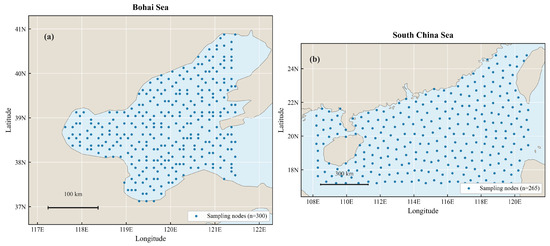
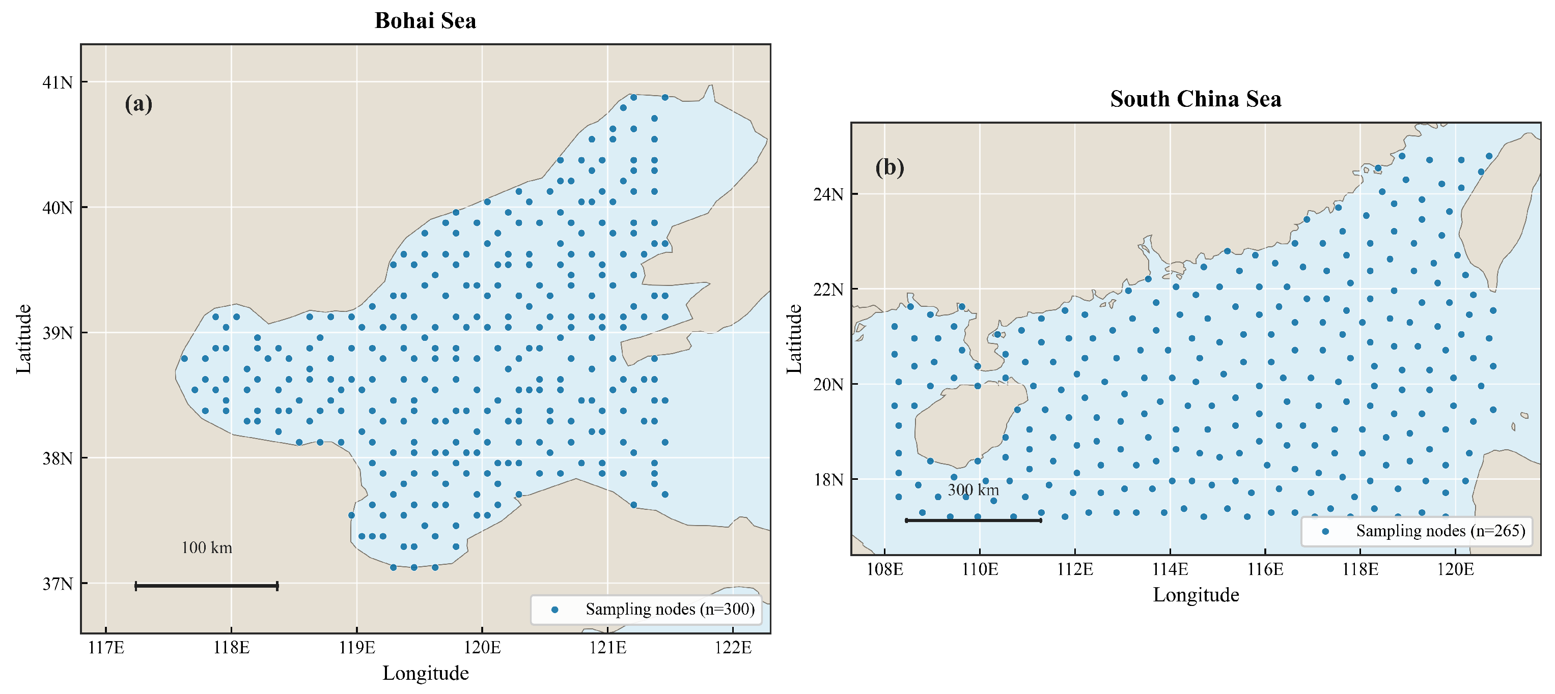
To evaluate forecasting performance under different marine water quality conditions, two representative regions were selected: the Bohai Sea and the South China Sea. The Bohai Sea is a semi-enclosed marginal sea strongly affected by coastal inputs, shallow-water processes, and human activities, whereas the South China Sea covers a broader marine region influenced by seasonal circulation and offshore processes. These two regions provide suitable test beds for evaluating multi-step Chl-a forecasting under different ecological and hydrodynamic conditions. The study areas and spatial distributions of Chl-a sampling nodes are shown in Figure 2.

For each region, spatial sampling nodes were extracted according to their latitude and longitude, and the daily Chl-a time series at these nodes were used for model training and evaluation. The dataset information is summarized in

Table 1. Summary of the Chl-a datasets.

Dataset	Temporal Coverage	Latitude Range	Longitude Range	Nodes
Bohai Sea	9 February 2018–30 August 2024	$37.12$–$40.{87}^{\circ }$ N	$117.63$–$121.{46}^{\circ }$ E	300
South China Sea	9 February 2018–16 October 2023	$17.21$–$24.{79}^{\circ }$ N	$108.21$–$120.{79}^{\circ }$ E	265

.

All datasets were chronologically split into training, validation, and test sets with a ratio of 70%, 10%, and 20%, respectively. A sliding-window strategy was adopted, using 30 days of historical Chl-a observations to predict the following 15 days. The chronological split ensured that future observations were not included in model training. Node coordinates were used for geographical graph construction and static feature representation.

4.2. Baseline Models

To evaluate the effectiveness of MS-STMoE, six recent spatio-temporal forecasting models were selected as baselines. These models cover graph diffusion networks, dynamic graph neural networks, heterogeneous spatio-temporal graph models, and Transformer-based architectures. Since marine Chl-a prediction can be formulated as a graph-based multi-node sequence forecasting task, these models provide suitable comparisons for evaluating temporal evolution and spatial dependency modeling. All baseline models were implemented under the same protocol as MS-STMoE, including identical data splits, input windows, forecasting horizons, preprocessing procedures, and evaluation metrics.

RGDAN: RGDAN combines random graph modeling, diffusion mechanisms, and attention modules to capture complex spatio-temporal dependencies [36].

DST-SGNN: DST-SGNN models dynamic graph structures under Stiefel manifold constraints for efficient spatio-temporal time series forecasting [37].

DVGNN: DVGNN integrates dynamic causal explanation, diffusion modeling, and variational graph learning to capture evolving spatial dependencies [38].

DSTAGNN: DSTAGNN dynamically constructs spatial-temporal aware graphs to model changing dependencies among spatial nodes [39].

HSTGNN: HSTGNN is designed to capture heterogeneous spatio-temporal dependencies among variables and spatial nodes [40].

STAEformer: STAEformer introduces spatio-temporal adaptive embeddings into a Transformer architecture for multi-node time series forecasting [41].

For fair comparison, all baseline models and the proposed model were evaluated on the original Chl-a concentration scale.

4.3. Evaluation Metrics and Experimental Settings

Mean absolute error (MAE) and root mean square error (RMSE) were adopted as evaluation metrics. Both metrics were calculated on the original Chl-a concentration scale after inverse standardization and inverse logarithmic transformation, and are reported in mg m⁻³. For multi-step forecasting, metrics were computed for each prediction step and then averaged over all forecasting steps.

Let ${\widehat{c}}_{s,h}^i$ and $c_{s,h}^i$ denote the predicted and observed Chl-a concentrations of node $v_i$ at the h-th forecasting step of test sample s, respectively. Let S denote the number of test samples, N denote the number of spatial nodes, and H denote the forecasting horizon. The step-wise MAE is defined as

$${\mathrm{MAE}}_h={\displaystyle \frac{1}{SN}}{\displaystyle \sum _{s=1}^S}{\displaystyle \sum _{i=1}^N}\left|{\widehat{c}}_{s,h}^i-c_{s,h}^i\right|,h=1,2,\dots ,H.$$

(34)

The step-wise RMSE is defined as

$${\mathrm{RMSE}}_h=\sqrt{{\displaystyle \frac{1}{SN}}{\sum }_{s=1}^S{\sum }_{i=1}^N{\left({\widehat{c}}_{s,h}^i-c_{s,h}^i\right)}^2},h=1,2,\dots ,H.$$

(35)

The average MAE and RMSE over all prediction steps are calculated as

$$\mathrm{MAE}={\displaystyle \frac{1}{H}}{\displaystyle \sum _{h=1}^H}{\mathrm{MAE}}_h,$$

(36)

$$\mathrm{RMSE}={\displaystyle \frac{1}{H}}{\displaystyle \sum _{h=1}^H}{\mathrm{RMSE}}_h.$$

(37)

A lower MAE indicates a smaller average absolute error, while a lower RMSE indicates fewer large deviations because RMSE is more sensitive to high-error predictions. Step-wise MAE and RMSE curves were also used to analyze error accumulation over the 15-day forecasting horizon.

For MS-STMoE, the latent dimension was set to 64, and the number of spatio-temporal representation layers was set to 2. Hyperparameters related to expert capacity, sparse routing, temporal convolution, graph connectivity, and auxiliary loss weights were selected according to validation performance and the sensitivity analysis in Section 4.7. The final dataset-specific settings are summarized in

Table 2. Dataset-specific hyperparameter settings of the proposed MS-STMoE model.

Dataset	Experts E	Top-k Routing ${\mathit{K}}_{\mathit{e}}$	Graph Neighbors ${\mathit{K}}_{\mathit{g}}$
Bohai Sea	8	3	12
South China Sea	6	4	6

.

The multi-scale temporal convolution module used three temporal branches. The kernel sizes and dilation rates were set to $[3, 5, 7]$ and $[1, 1, 2]$ for the Bohai Sea dataset, and $[3, 7, 9]$ and $[1, 2, 4]$ for the South China Sea dataset, respectively. Unless otherwise specified, the model was trained using the AdamW optimizer with a learning rate of $1\times {10}^{-3}$, weight decay of $1\times {10}^{-4}$, batch size of 16, and Huber loss with $\delta =1.0$. The router z-loss weight was set to ${\lambda }_z=0.001$ for both datasets, while the expert balance loss weight ${\lambda }_b$ was set to $0.01$ for the Bohai Sea dataset and $0.0003$ for the South China Sea dataset. The MoE residual scaling coefficient was initialized to $0.3$, and a 10-epoch residual warm-up was used. Router noise was used during training and disabled during evaluation. Early stopping with a patience of 10 epochs was adopted based on the validation loss, and the random seed was fixed to 42.

4.4. Multi-Step Forecasting Performance

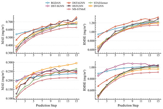
To evaluate forecasting performance under increasing prediction horizons, the step-wise MAE and RMSE values over the 15-day forecasting horizon were compared on the Bohai Sea and South China Sea datasets.

Table 3. Multi-step forecasting performance on the two datasets. Each cell reports MAE/RMSE in mg m⁻³.

Dataset	Model	Step 1	Step 3	Step 5	Step 7	Step 9	Step 11	Step 13	Step 15	Avg.
Bohai Sea	RGDAN	0.540/0.944	0.568/1.008	0.593/1.071	0.614/1.114	0.633/1.151	0.650/1.182	0.665/1.207	0.678/1.231	0.618/1.116
	DST-SGNN	0.369/0.640	0.449/0.813	0.520/0.951	0.571/1.038	0.604/1.100	0.655/1.158	0.664/1.186	0.678/1.211	0.568/1.020
	DVGNN	0.390/0.669	0.490/0.835	0.545/0.953	0.592/1.037	0.626/1.098	0.657/1.147	0.678/1.178	0.691/1.193	0.587/1.021
	DSTAGNN	0.469/0.891	0.557/1.019	0.600/1.123	0.638/1.169	0.673/1.236	0.703/1.275	0.688/1.275	0.759/1.328	0.634/1.168
	HSTGNN	0.336/0.555	0.477/0.815	0.563/1.008	0.601/1.076	0.657/1.160	0.673/1.193	0.717/1.250	0.734/1.286	0.600/1.052
	STAEformer	0.329/0.621	0.485/0.845	0.525/0.946	0.576/1.054	0.615/1.125	0.654/1.197	0.674/1.222	0.667/1.230	0.570/1.038
	MS-STMoE	0.316/0.599	0.429/0.802	0.506/0.939	0.549/1.025	0.581/1.081	0.609/1.125	0.629/1.142	0.628/1.149	0.536/0.992
South China Sea	RGDAN	0.200/0.889	0.210/0.930	0.218/0.964	0.224/0.985	0.229/0.998	0.232/1.009	0.235/1.018	0.238/1.021	0.224/0.979
	DST-SGNN	0.194/0.853	0.221/0.961	0.234/1.011	0.246/1.057	0.251/1.062	0.252/1.057	0.248/1.030	0.248/1.018	0.239/1.014
	DVGNN	0.165/0.507	0.212/0.685	0.241/0.797	0.258/0.881	0.270/0.931	0.277/0.957	0.286/0.970	0.296/0.967	0.253/0.846
	DSTAGNN	0.156/0.675	0.185/0.774	0.239/0.854	0.228/0.909	0.238/0.952	0.241/0.985	0.249/0.999	0.244/1.008	0.224/0.899
	HSTGNN	0.125/0.510	0.181/0.688	0.210/0.809	0.240/0.906	0.254/0.974	0.249/0.988	0.253/1.017	0.253/1.032	0.228/0.875
	STAEformer	0.109/0.480	0.166/0.679	0.202/0.809	0.221/0.902	0.231/0.956	0.244/0.982	0.250/0.998	0.264/1.001	0.212/0.860
	MS-STMoE	0.105/0.472	0.153/0.663	0.182/0.771	0.200/0.846	0.210/0.884	0.213/0.899	0.214/0.908	0.214/0.914	0.189/0.804

Note: Bold numerical values indicate the best (lowest) result for each metric at each forecasting step and for the average within each dataset.

reports the quantitative results at representative odd prediction steps, together with the average errors over all 15 steps. Figure 3 further shows the complete error evolution curves.

As shown in Table 3, MS-STMoE achieves the lowest average MAE and RMSE on both datasets. On the Bohai Sea dataset, MS-STMoE obtains an average MAE of 0.536 and an average RMSE of 0.992, outperforming the second-best model DST-SGNN by approximately 5.6% and 2.7%, respectively. On the South China Sea dataset, MS-STMoE reduces the average MAE from 0.212 to 0.189 compared with STAEformer and the average RMSE from 0.846 to 0.804 compared with DVGNN, corresponding to improvements of approximately 11.0% and 5.0%, respectively.

The step-wise results further show that MS-STMoE maintains stable performance as the forecasting horizon increases. In the Bohai Sea, several baseline models remain competitive at very short horizons, especially in terms of RMSE, whereas MS-STMoE becomes more advantageous from the medium-term prediction steps onward. This is relevant for marine water quality monitoring because short- to medium-term Chl-a prediction is often needed for early warning and management responses. In the South China Sea, MS-STMoE achieves the best MAE and RMSE at all reported odd prediction steps, indicating robust performance across the forecasting horizon.

Figure 3 visualizes the complete 15-step error evolution. Prediction errors generally increase with the forecasting horizon, reflecting the accumulation of uncertainty in multi-step prediction. Compared with the baseline models, MS-STMoE exhibits lower and smoother error curves, especially in the South China Sea. For the Bohai Sea, MS-STMoE maintains the lowest MAE across the forecasting horizon and shows clearer RMSE advantages after the short-term prediction steps.

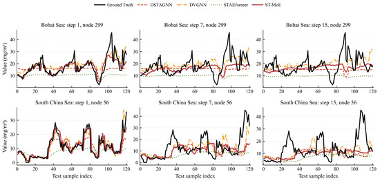
To further examine temporal forecasting behavior, Figure 4 presents representative fitting curves at prediction steps 1, 7, and 15. MS-STMoE follows the temporal variations in the ground truth more closely in most cases and better preserves Chl-a fluctuation patterns. Several displayed extreme peaks are nevertheless underestimated, which may reflect both the absence of contemporaneous environmental drivers and the use of logarithmic transformation and Huber loss, which improve robustness but reduce the influence of abrupt high-concentration values during training.

The increasing advantage at medium-to-late forecast horizons is consistent with the combined contribution of multi-scale temporal convolution and seasonal encoding: multi-scale receptive fields represent temporal variations over different ranges, while seasonal encoding provides periodic information as the forecast horizon increases. Sparse routing further supplies node-conditioned refinement, although the subsequent ablation and node-level analyses show that its incremental contribution is modest and region-dependent. Overall, the horizon-wise advantage should therefore be attributed to the complete framework rather than to the MoE module alone.

The spatial distribution of prediction errors is further analyzed in the following subsection to examine model performance across different marine nodes.

4.5. Spatial Error Distribution and Expert Routing Analysis

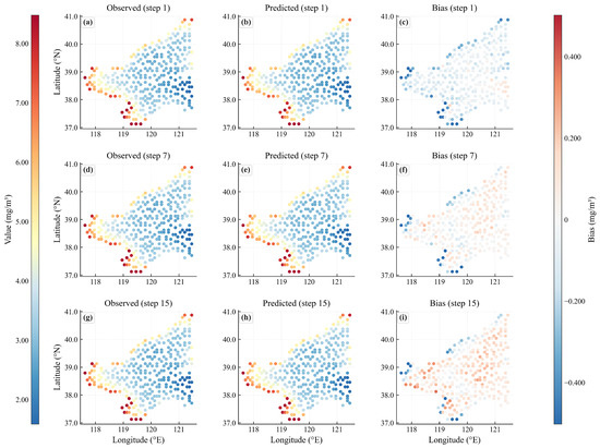
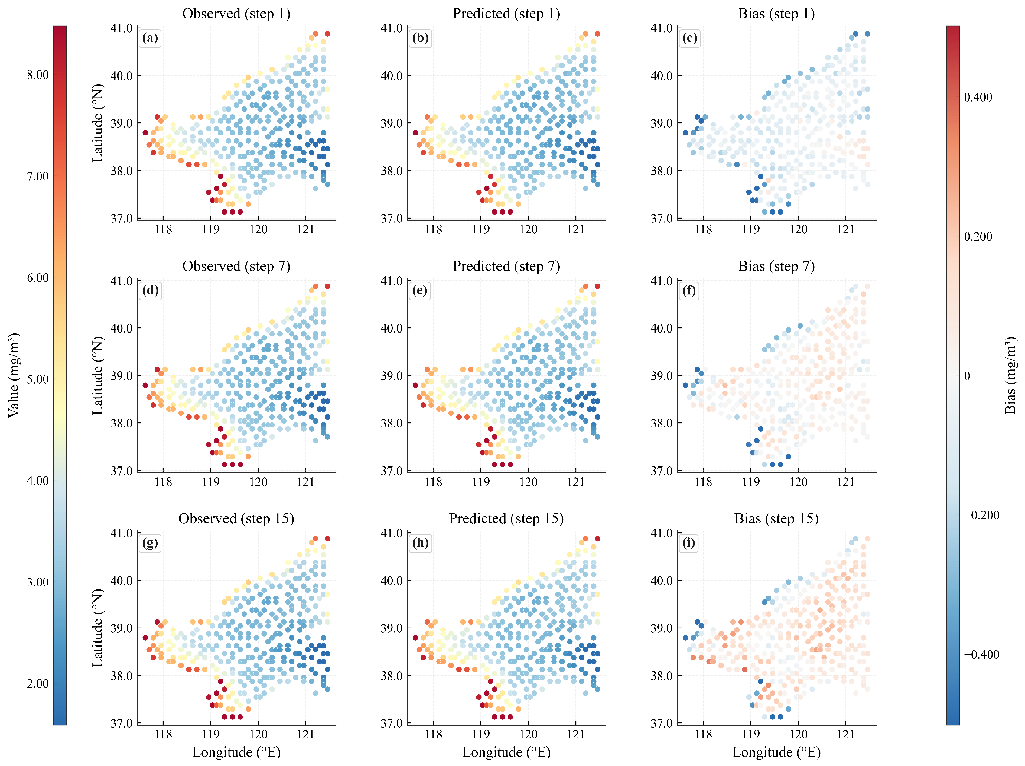
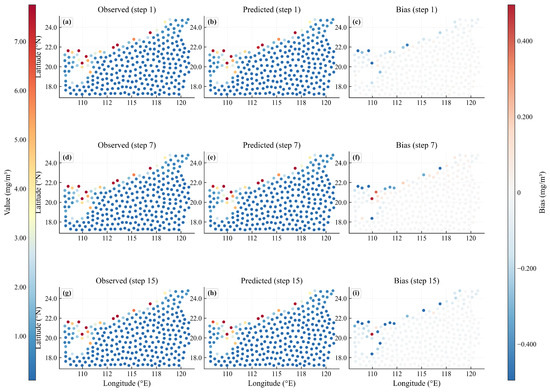
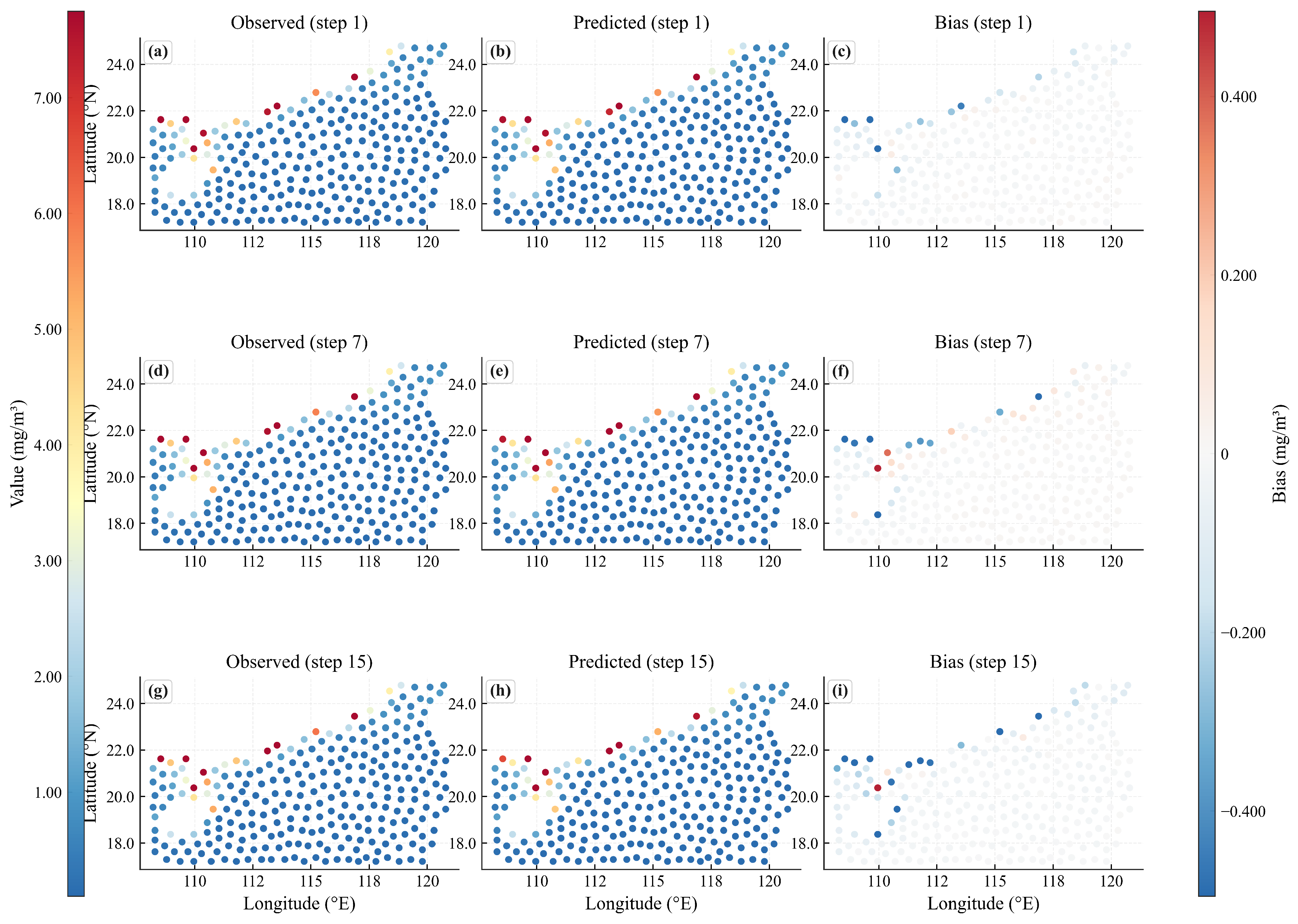
Step-wise MAE and RMSE quantify overall forecasting accuracy, but they do not reveal how prediction errors are distributed across marine nodes. For marine water quality monitoring, spatial error behavior is important because large local errors may occur in coastal or high-Chl-a regions even when the overall average error is low. To examine the spatial behavior of MS-STMoE, Figure 5 and Figure 6 present the test-set mean observed fields, predicted fields, and prediction bias at prediction steps 1, 7, and 15 for the Bohai Sea and South China Sea datasets, respectively.

Figure 5 shows that MS-STMoE captures the principal spatial gradient of Bohai Sea Chl-a, although localized biases become more visible near coastal or high-concentration nodes at longer horizons because sharp local variations and unobserved environmental forcing are more difficult to extrapolate from historical Chl-a and geographical adjacency alone.

Figure 6 shows that MS-STMoE reproduces the dominant low-concentration background of the South China Sea without producing large continuous error regions, while several localized concentration peaks remain comparatively difficult to predict.

To further quantify node-level spatial error distribution, node-wise MAE was calculated over all test samples and forecasting steps:

$${\mathrm{MAE}}_i^{\mathrm{node}}={\displaystyle \frac{1}{SH}}{\displaystyle \sum _{s=1}^S}{\displaystyle \sum _{h=1}^H}\left|{\widehat{c}}_{s,h}^i-c_{s,h}^i\right|,$$

(38)

where S is the number of test samples, H is the forecasting horizon, and i denotes the spatial node index. The node-wise MAE measures the average local forecasting error at each marine node.

For a paired comparison at the same spatial locations, the MAE difference between a comparison model b and MS-STMoE was defined for node i as

$${\Delta }_i^{\left(b\right)}={\mathrm{MAE}}_i^{\left(b\right)}-{\mathrm{MAE}}_i^{\left(\mathrm{M}\mathrm{S-}\mathrm{S}\mathrm{T}\mathrm{M}\mathrm{o}\mathrm{E}\right)}.$$

(39)

A positive value indicates a lower node-wise MAE for MS-STMoE; the P95 node error was additionally calculated at each prediction step, and the mean P95 gain represents its average relative reduction over the 15-step horizon.

Table 4. Node-wise MAE improvements and P95 high-error-tail comparisons.

Dataset	Comparison	Mean ΔMAE	Median ΔMAE	Improved Nodes	P95 Improved Steps	Mean P95 Gain
Bohai Sea	vs. STAEformer	0.0340	0.0473	96.67%	15/15	6.55%
Bohai Sea	vs. w/o MoE	0.0060	0.0032	55.67%	9/15	$-1.47\%$
South China Sea	vs. STAEformer	0.0230	0.0294	100%	15/15	16.70%
South China Sea	vs. w/o MoE	0.0035	0.0032	83.40%	1/15	$-1.82\%$

shows that the complete MS-STMoE framework outperforms STAEformer at 96.67% of the Bohai Sea nodes and all South China Sea nodes and reduces the P95 error at all 15 prediction steps, demonstrating that its overall advantage extends to most individual nodes and high-error locations.

Compared with the w/o MoE variant, sparse routing improves 55.67% and 83.40% of the nodes in the two regions, respectively, but its small mean MAE differences and negative mean P95 gains indicate that the incremental improvement is modest and does not consistently extend to the high-error tail.

To examine the mechanism underlying this incremental effect, the test-set-averaged routing weight and dominant expert of each node were defined as

$${\overline{g}}_{i,e}={\displaystyle \frac{1}{S}}{\displaystyle \sum _{s=1}^S}{g}_{s,i,e},e_i^{*}=\arg \underset{e}{\max }{\overline{g}}_{i,e},$$

(40)

where $g_{s,i,e}$ is the deterministic sparse routing weight assigned to expert e for node i in test sample s.

Global expert loads were obtained by averaging the deterministic routing weights over all test samples and nodes, and their Shannon entropy was normalized by $\log E$ so that a value of one represents uniform expert utilization.

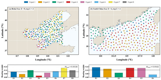
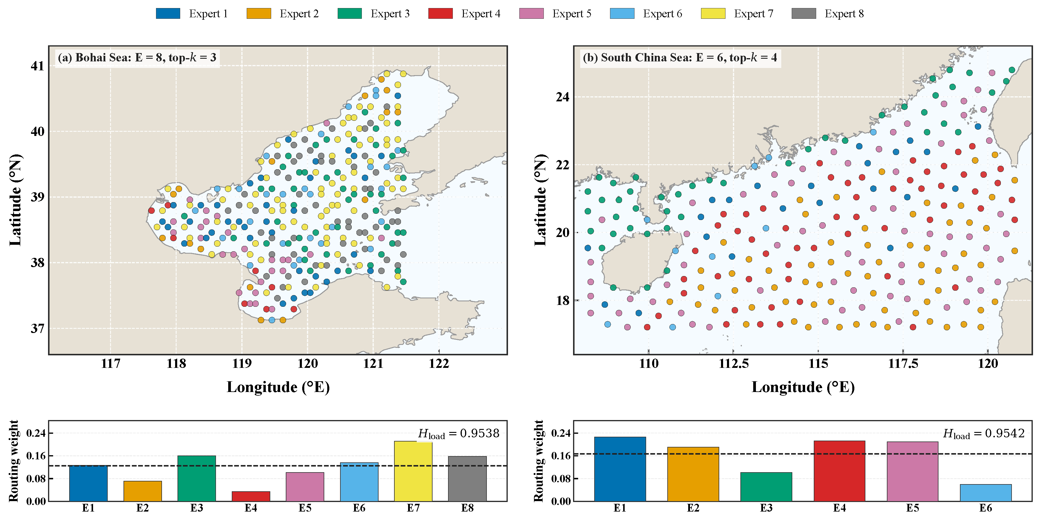
Figure 7 shows differentiated and locally structured expert utilization, with four-nearest-neighbor agreement reaching 1.31 and 1.69 times the random expectation and normalized global load entropies of 0.9538 and 0.9542 in the Bohai Sea and South China Sea, respectively, indicating that spatially varying routing is achieved without evident expert collapse.

The routing results support the use of node-differentiated prediction pathways but do not establish a direct causal relationship between individual expert assignments and error reduction; therefore, sparse routing is interpreted as a node-adaptive refinement mechanism with modest, region-dependent gains, while the broader node-level and high-error-tail improvements arise from the combined contribution of the complete MS-STMoE framework.

4.6. Ablation Study

To evaluate the contribution of each component, ablation experiments were conducted by removing the MoE module, seasonal encoding, and multi-scale TCN module, respectively. The results are reported in

Table 5. Ablation study results. Each cell reports MAE/RMSE in mg m⁻³.

Dataset	Variant	MAE				RMSE
		Step 1	Step 7	Step 15	Avg.	Step 1	Step 7	Step 15	Avg.
Bohai Sea	MS-STMoE	0.316	0.549	0.628	0.536	0.599	1.025	1.149	0.992
	w/o MoE	0.306	0.563	0.632	0.542	0.576	1.029	1.160	0.991
	w/o Seasonal Encoding	0.318	0.567	0.650	0.552	0.597	1.059	1.211	1.027
	w/o Multi-scale TCN	0.342	0.549	0.634	0.540	0.621	1.046	1.183	1.013
South China Sea	MS-STMoE	0.105	0.200	0.214	0.189	0.472	0.846	0.914	0.804
	w/o MoE	0.110	0.206	0.218	0.192	0.488	0.853	0.921	0.816
	w/o Seasonal Encoding	0.101	0.206	0.236	0.197	0.468	0.882	0.980	0.846
	w/o Multi-scale TCN	0.112	0.205	0.221	0.194	0.486	0.854	0.907	0.809

Note: Bold numerical values indicate the best (lowest) result in each column for each dataset; tied best values are also shown in bold.

.

On the Bohai Sea dataset, the complete MS-STMoE model achieves the lowest average MAE and obtains the best MAE at steps 7 and 15. Removing seasonal encoding causes the most evident degradation, increasing the average MAE from 0.536 to 0.552 and the average RMSE from 0.992 to 1.027. This indicates that seasonal information is important for Chl-a forecasting in a semi-enclosed marginal sea where periodic environmental forcing can affect phytoplankton variability. Removing the multi-scale TCN also increases the average RMSE to 1.013, showing that multi-scale temporal modeling contributes to medium- and long-term forecasting. Although the w/o MoE variant obtains a slightly lower average RMSE, its average MAE and medium- to long-term errors are worse, indicating that the MoE module provides a small MAE-oriented refinement in this region without consistently improving every metric.

On the South China Sea dataset, the complete MS-STMoE model achieves the lowest average MAE and RMSE among all variants. Removing the MoE module increases the average MAE from 0.189 to 0.192 and the average RMSE from 0.804 to 0.816, indicating a modest but more consistent average-error improvement in the South China Sea. Removing seasonal encoding leads to the largest RMSE degradation, especially at medium- and long-term prediction steps. The w/o Multi-scale TCN variant obtains a slightly lower RMSE at step 15, but its average MAE and RMSE are both worse than those of the complete model.

Overall, seasonal encoding produces the largest average degradation when removed from either dataset, confirming the importance of periodic information in both regions. The contribution of multi-scale temporal convolution varies across metrics and forecast steps, while sparse routing provides a smaller, region-dependent refinement that is more consistent in the South China Sea. The components should therefore be interpreted as complementary, with seasonal and multi-scale representations forming the main forecasting foundation and MoE providing node-adaptive adjustment.

4.7. Parameter Sensitivity Analysis

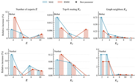
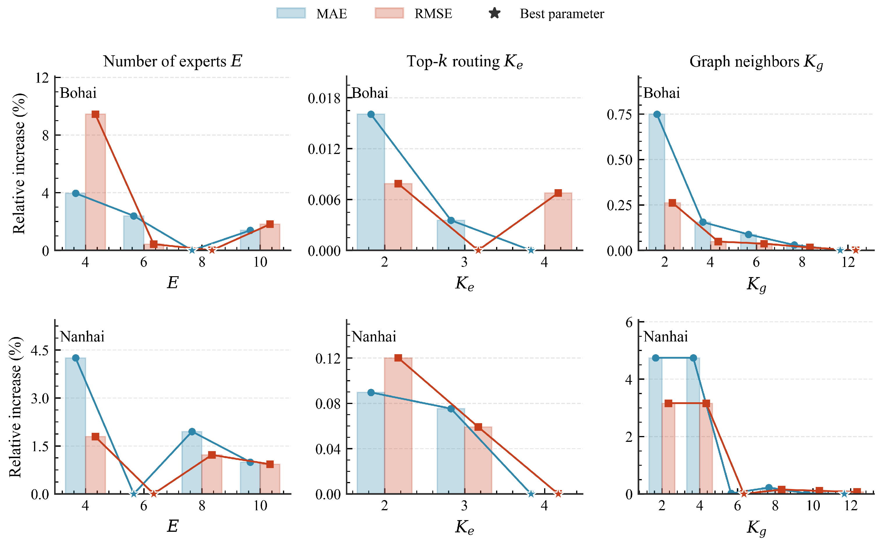
To examine the influence of key hyperparameters on the proposed model, sensitivity experiments were conducted on three important settings: the number of experts E, the top-k routing number $K_e$, and the number of graph neighbors $K_g$. These parameters correspond to expert capacity, routing sparsity, and spatial graph construction, respectively.

For clearer comparison, the relative increase in each metric under different parameter settings was calculated with respect to the best result within the same parameter group:

$${\Delta }_m\left(p\right)={\displaystyle \frac{m\left(p\right)-{\min }_{p}m\left(p\right)}{{\min }_{p}m\left(p\right)}}\times 100\%,$$

(41)

where $m\in \{\mathrm{MAE},\mathrm{RMSE}\}$, and a smaller value indicates better performance. In Figure 8, blue bars denote the relative increase in MAE, orange bars denote the relative increase in RMSE, and stars indicate the selected best parameter settings.

As shown in Figure 8, the optimal hyperparameter settings differ between the two study regions. For the number of experts, the best settings are $E=8$ for the Bohai Sea and $E=6$ for the South China Sea, indicating that expert capacity should be adjusted according to dataset-specific representation requirements. When the number of experts is too small, the model may not have sufficient capacity to represent diverse Chl-a variation patterns, whereas too many experts may introduce unnecessary complexity.

The top-k routing number controls how many experts are activated for each node representation. The best settings are $K_e=3$ for the Bohai Sea and $K_e=4$ for the South China Sea, suggesting that moderate routing sparsity helps balance expert specialization and representation flexibility. For graph connectivity, the Bohai Sea obtains the best result when $K_g=12$, whereas the South China Sea performs best when $K_g=6$. The larger neighborhood in the Bohai Sea may reflect the benefit of aggregating information from more nearby nodes under its spatial sampling configuration, whereas the smaller neighborhood in the South China Sea may help limit excessive smoothing across more widely distributed locations.

Based on the sensitivity results, the final settings are $E=8$, $K_e=3$, and $K_g=12$ for the Bohai Sea dataset, and $E=6$, $K_e=4$, and $K_g=6$ for the South China Sea dataset. These results indicate that the balance between expert capacity, routing sparsity, and graph connectivity is dataset-dependent. Because the parameters were selected empirically on the validation sets, they should not be interpreted as direct evidence that particular experts or graph neighborhoods correspond to specific ecological or hydrodynamic processes.

4.8. Comparative Discussion and Limitations

Previous Transformer- and graph-based Chl-a forecasting studies have demonstrated the value of nonlinear spatio-temporal representation learning for marine environmental prediction [9,10,11,12]. The present results are consistent with this general finding, as geographical graph modeling and multi-scale temporal representation enable MS-STMoE to outperform six recent spatio-temporal baselines under a common evaluation protocol. Direct numerical comparison with previously published accuracy values is difficult because the datasets, spatial resolutions, input variables, and forecasting horizons differ across studies. The additional contribution of this study is therefore not limited to domain-averaged accuracy but also includes paired node-wise and P95 analyses that clarify how broadly the improvements are distributed across marine locations.

Sparse expert routing has previously been used to address heterogeneous spatial prediction behavior in traffic forecasting [17]. The present study extends this idea to marine Chl-a forecasting by showing that different marine nodes form spatially structured expert-utilization patterns without evident expert collapse. However, the ablation results indicate that the incremental accuracy gain of MoE is modest and region-dependent, suggesting that sparse routing should complement rather than replace geographical graph modeling, multi-scale temporal representation, and seasonal encoding. The learned experts are data-driven subnetworks and cannot be directly interpreted as predefined water masses or ecological regimes.

This study has several limitations. First, the model does not incorporate contemporaneous environmental covariates such as sea surface temperature, wind, currents, or nutrient conditions, which may limit its ability to predict abrupt Chl-a changes. Second, the experiments cover only two marine regions, and broader multi-region evaluation is needed to assess transferability under different spatial sampling configurations and environmental conditions. Third, the routing analysis establishes differentiated expert utilization but not a causal relationship between expert selection and node-level error reduction. Future work may integrate multi-source environmental observations and physics-informed constraints into the routing mechanism and evaluate its generalizability across additional marine regions.

5. Conclusions

This study proposed MS-STMoE, a multi-scale spatio-temporal mixture-of-experts framework for heterogeneity-aware multi-step Chl-a forecasting in marine water quality monitoring. By integrating geographical graph modeling, multi-scale temporal convolution, and sparse expert routing, the proposed model captures spatial dependencies, temporal variations, and region-specific Chl-a dynamics within a unified forecasting framework and supports node-adaptive forecasting under heterogeneous marine conditions.

Experiments on the Bohai Sea and South China Sea datasets show that MS-STMoE improves multi-step forecasting accuracy and preserves the main spatial distribution patterns of Chl-a. Compared with the best-performing baseline models, the proposed framework reduces the average MAE/RMSE by approximately 5.6%/2.7% in the Bohai Sea and 11.0%/5.0% in the South China Sea, respectively. Node-wise analyses further show broad improvements relative to STAEformer, whereas the additional gains of the MoE module are modest and region-dependent. The ablation and sensitivity analyses indicate complementary component roles: seasonal encoding and multi-scale temporal modeling provide the main forecasting support, while sparse expert routing contributes a node-adaptive refinement. Overall, these results demonstrate the usefulness of heterogeneity-aware modeling for short- to medium-term Chl-a forecasting under different marine water quality conditions.

Several limitations remain. The current model mainly uses historical Chl-a observations and seasonal encodings, while physical and biogeochemical variables such as sea surface temperature, salinity, wind, nutrients, and ocean currents are not explicitly incorporated. In addition, the geographical graph is constructed from static node distances and may not fully represent dynamic ocean transport processes. The current evaluation covers two representative marine regions, and the routing analysis does not establish a direct causal relationship between individual expert assignments and node-level error reduction. Future work will incorporate multi-source environmental variables, dynamic ocean-aware graph structures, and event-level validation strategies to improve the prediction of abrupt Chl-a changes and support region-aware short- to medium-term marine water quality monitoring.

References

- Hong, Z.; Long, D.; Shan, K.; Zhang, J.M.; Woolway, R.I.; Liu, M.; Mann, M.E.; Fang, H. Declining ocean greenness and phytoplankton blooms in low- to mid-latitudes under a warming climate. Sci. Adv. 2025, 11, eadx4857. [Google Scholar] [CrossRef] [Scilit] [PubMed]
- Martinez Balbontin, G.; Jouanno, J.; Benshila, R.; Lamouroux, J.; Perruche, C.; Ciavatta, S. Forecasting seasonal global sea surface chlorophyll a with a lightweight data-driven approach. Biogeosciences 2026, 23, 2601–2620. [Google Scholar] [CrossRef] [Scilit]
- Zhang, F.; Kung, H.; Zhang, F.; Yang, C.; Gan, J. AI-powered spatiotemporal imputation and prediction of chlorophyll-a concentration in coastal ecosystems. Nat. Commun. 2025, 16, 7656. [Google Scholar] [CrossRef] [Scilit] [PubMed]
- Ruan, Q.; Pan, D.; Wang, D.; He, X.; Gong, F.; Tian, Q. Prediction of sea surface chlorophyll-a concentrations by remote sensing and deep learning. Remote Sens. 2025, 17, 1755. [Google Scholar] [CrossRef] [Scilit]
- Ding, W.; Zhang, C.; Li, X.; Zhang, L.; Chen, N. Enhanced forecasting of coastal chlorophyll-a through AdaBoost-optimized LSTM models. Acta Oceanol. Sin. 2025, 44, 147–160. [Google Scholar] [CrossRef] [Scilit]
- Liu, N.; Chen, S.; Cheng, Z.; Xing, W.; Yun, X.; Li, X.; Guo, Y.; Wang, T.; Zhang, X.; Li, S. Long-term prediction of sea surface chlorophyll-a concentration based on the combination of spatio-temporal features. Water Res. 2022, 211, 118040. [Google Scholar] [CrossRef] [Scilit] [PubMed]
- Huang, H.; Zhang, J. Prediction of chlorophyll a and risk assessment of water blooms in Poyang Lake based on a machine learning method. Environ. Pollut. 2024, 347, 123501. [Google Scholar] [CrossRef] [Scilit] [PubMed]
- Yao, L.; Wang, X.; Zhang, J.; Yu, X.; Zhang, S.; Li, Q. Prediction of sea surface chlorophyll-a concentrations based on deep learning and time-series remote sensing data. Remote Sens. 2023, 15, 4486. [Google Scholar] [CrossRef] [Scilit]
- Sun, X.; Yan, D.; Wu, S.; Chen, Y.; Qi, J.; Du, Z. Enhanced forecasting of chlorophyll-a concentration in coastal waters through integration of Fourier analysis and Transformer networks. Water Res. 2024, 263, 122160. [Google Scholar] [CrossRef] [Scilit] [PubMed]
- Zhou, G.; Liu, M.; Li, L. A spatiotemporal fusion transformer model for chlorophyll-a concentrations prediction over large areas with satellite time series data. IEEE Trans. Geosci. Remote Sens. 2024, 62, 4210211. [Google Scholar] [CrossRef] [Scilit]
- Yoon, S.; Ahn, K.H. Improved prediction of chlorophyll-a concentrations using advancing graph neural network variants. Sci. Total Environ. 2025, 979, 179481. [Google Scholar] [CrossRef] [Scilit] [PubMed]
- Zarbipour, P.; Akbari, H.; Nikoo, M.R.; Choolanak, A.K. Spatiotemporal prediction of chlorophyll-a in semi-enclosed gulfs using a hybrid graph neural network-transformer framework with satellite data and causal analysis. Sci. Rep. 2026, 16, 13973. [Google Scholar] [CrossRef] [Scilit] [PubMed]
- Kim, H.; Kim, B.G.; Kim, K.J.; Kim, T.-H.; Shin, H.-K.; Han, J.H. Chlorophyll-a prediction based on machine learning and satellite data in the South Sea of Korea. IEEE J. Sel. Top. Appl. Earth Obs. Remote Sens. 2025, 18, 19066–19075. [Google Scholar] [CrossRef] [Scilit]
- Kim, S.; Lee, D.; Kim, M.; Jang, H.K.; Park, S.; Kim, Y.; Kim, J.; Park, J.W.; Joo, H.; Lee, S.H. Seasonal patterns and bloom dynamics of phytoplankton based on satellite-derived chlorophyll-a in the eastern Yellow Sea. Mar. Environ. Res. 2024, 199, 106605. [Google Scholar] [CrossRef] [Scilit] [PubMed]
- Liu, M.; Gu, B.; Liu, C.; Su, B.; Meng, Q.; Zhang, Y.; Li, M. Phenological patterns and driving mechanisms of autumn phytoplankton blooms in the Yellow Sea Cold Water Mass (2000–2022). J. Mar. Sci. Eng. 2026, 14, 313. [Google Scholar] [CrossRef] [Scilit]
- Ni, R.; Lin, Z.; Wang, S.; Fanti, G. Mixture-of-linear-experts for long-term time series forecasting. In Proceedings of the International Conference on Artificial Intelligence and Statistics, Valencia, Spain, 2–4 May 2024; pp. 4672–4680. [Google Scholar]
- Li, S.; Cui, Y.; Zhao, Y.; Yang, W.; Zhang, R.; Zhou, X. ST-MoE: Spatio-temporal mixture-of-experts for debiasing in traffic prediction. In Proceedings of the 32nd ACM International Conference on Information and Knowledge Management; Association for Computing Machinery: New York, NY, USA, 2023; pp. 1208–1217. [Google Scholar]
- Sukkuea, A.; Akkajit, P.; Suwannarat, K.; Foithong, P.; Afsarimanesh, N.; Alahi, M.E.E. AI-driven time series forecasting of coastal water quality using Sentinel-2 imagery: A case study in the Gulf of Thailand. Water 2025, 17, 1798. [Google Scholar] [CrossRef] [Scilit]
- Wang, W.; Hu, X.; Meng, H.; Liu, C.; Wang, Y.; Jiao, T.; Chang, Q.; Lai, B. Machine learning-based prediction and interpretability analysis of chlorophyll-a and algal density using high-frequency water quality data. Diversity 2026, 18, 282. [Google Scholar] [CrossRef] [Scilit]
- Zhang, C.; Ding, W.; Zhang, L. Impacts of missing buoy data on LSTM-based coastal chlorophyll-a forecasting. Water 2024, 16, 3046. [Google Scholar] [CrossRef] [Scilit]
- Gupta, S.; Gupta, S. Time series forecasting of chlorophyll-a concentrations in the Chesapeake Bay. Sci. Rep. 2025, 15, 30877. [Google Scholar] [CrossRef] [Scilit] [PubMed]
- Hong, Z.; Long, D.; Li, X.; Wang, Y.; Zhang, J.; Hamouda, M.A.; Mohamed, M.M. A global daily gap-filled chlorophyll-a dataset in open oceans during 2001–2021 from multisource information using convolutional neural networks. Earth Syst. Sci. Data 2023, 15, 5281–5300. [Google Scholar] [CrossRef] [Scilit]
- Gilerson, A.; Malinowski, M.; Agagliate, J.; Herrera-Estrella, E.; Tzortziou, M.; Tomlinson, M.C.; Meredith, A.; Stumpf, R.P.; Ondrusek, M.; Jiang, L.; et al. Development of VIIRS-OLCI chlorophyll-a product for the coastal estuaries. Front. Mar. Sci. 2024, 11, 1476425. [Google Scholar] [CrossRef] [Scilit]
- Liu, X.; Wang, M. Global daily gap-free ocean color products from multi-satellite measurements. Int. J. Appl. Earth Obs. Geoinf. 2022, 108, 102714. [Google Scholar] [CrossRef] [Scilit]
- Zhao, Y.; Yang, D.; He, J.; Zhu, K.; Deng, X. Hierarchical stacked spatiotemporal self-attention network for sea surface temperature forecasting. Ocean Model. 2024, 191, 102427. [Google Scholar] [CrossRef] [Scilit]
- Song, D.; Dai, S.; Li, W.; Ren, T.; Wei, Z.; Liu, A.-A. STVformer: A spatial-temporal-variable transformer with auxiliary knowledge for sea surface temperature prediction. Appl. Ocean Res. 2024, 153, 104218. [Google Scholar] [CrossRef] [Scilit]
- Sainsbury-Dale, M.; Zammit-Mangion, A.; Richards, J.; Huser, R. Neural Bayes estimators for irregular spatial data using graph neural networks. J. Comput. Graph. Stat. 2025, 34, 1153–1168. [Google Scholar] [CrossRef] [Scilit]
- Peng, B.; Hong, Z.; Wang, G. A hybrid Mamba–ConvLSTM framework for multi-day sea surface temperature forecasting at 0.05 degree resolution. J. Mar. Sci. Eng. 2026, 14, 898. [Google Scholar] [CrossRef] [Scilit]
- Li, Z.; Sun, D.; Wang, S.; Huan, Y.; Zhang, H.; Yuan, Y.; He, Y. Ocean-scale patterns of environment and climate changes driving global marine phytoplankton biomass dynamics. Sci. Adv. 2024, 10, eadm7556. [Google Scholar] [CrossRef] [Scilit] [PubMed]
- Shafeeque, M.; Saleem, A.A.; Chaitanya, A.V.S.; Abdulla, C.P.; Lateef, S.; Albert, J. Chlorophyll-a modulation in the Arabian Gulf using two decades of merged ocean-color data. Front. Mar. Sci. 2025, 12, 1619821. [Google Scholar] [CrossRef] [Scilit]
- Xu, M.; Wang, Y.; Feng, Z.; Wu, H. Rapid variations of phytoplankton blooms and their dynamics off the Changjiang River Estuary. Front. Mar. Sci. 2024, 11, 1345940. [Google Scholar] [CrossRef] [Scilit]
- Zhu, Q.; Lee, Z. Offshore high chlorophyll eddies: Separating upwelling from nearshore migration from ocean color remote sensing. Prog. Oceanogr. 2024, 223, 103232. [Google Scholar] [CrossRef] [Scilit]
- Li, D.; Ruan, X.; Le-Quy Pham, A.; Damien, P.; Bianchi, D. Role of eddies in primary production in the California Current System. Geophys. Res. Lett. 2025, 52, e2025GL118614. [Google Scholar] [CrossRef] [Scilit]
- Alkilane, K.; He, Y.; Lee, D.H. MixMamba: Time series modeling with adaptive expertise. Inf. Fusion 2024, 112, 102589. [Google Scholar] [CrossRef] [Scilit]
- Shi, X.; Wang, S.; Nie, Y.; Li, D.; Ye, Z.; Wen, Q.; Jin, M. Time-MoE: Billion-scale time series foundation models with mixture of experts. arXiv 2024, arXiv:2409.16040. [Google Scholar]
- Fan, J.; Weng, W.; Tian, H.; Wu, H.; Zhu, F.; Wu, J. RGDAN: A random graph diffusion attention network for traffic prediction. Neural Netw. 2024, 172, 106093. [Google Scholar] [CrossRef] [Scilit] [PubMed]
- Zheng, J.; Xie, L. A dynamic Stiefel graph neural network for efficient spatio-temporal time series forecasting. arXiv 2025, arXiv:2506.00798. [Google Scholar]
- Liang, G.; Tiwari, P.; Nowaczyk, S.; Byttner, S.; Alonso-Fernandez, F. Dynamic causal explanation based diffusion-variational graph neural network for spatiotemporal forecasting. IEEE Trans. Neural Netw. Learn. Syst. 2025, 36, 9524–9537. [Google Scholar] [CrossRef] [Scilit] [PubMed]
- Lan, S.; Ma, Y.; Huang, W.; Wang, W.; Yang, H.; Li, P. DSTAGNN: Dynamic spatial-temporal aware graph neural network for traffic flow forecasting. In Proceedings of the International Conference on Machine Learning; PMLR: Cambridge, MA, USA, 2022; pp. 11906–11917. [Google Scholar]
- Zhang, Y.; Li, Z.; Chen, Z.; Qi, Y.; Gui, N. Heterogeneous Spatial Temporal Graph Neural Network for Multivariate Time Series Forecasting. In Proceedings of the IEEE International Conference on Acoustics, Speech and Signal Processing (ICASSP), Barcelona, Spain, 3–8 May 2026; pp. 4356–4360. [Google Scholar]
- Liu, H.; Dong, Z.; Jiang, R.; Deng, J.; Deng, J.; Chen, Q.; Song, X. Spatio-temporal adaptive embedding makes vanilla transformer SOTA for traffic forecasting. In Proceedings of the 32nd ACM International Conference on Information and Knowledge Management; Association for Computing Machinery: New York, NY, USA, 2023; pp. 4125–4129. [Google Scholar]
Disclaimer/Publisher’s Note: The statements, opinions and data contained in all publications are solely those of the individual author(s) and contributor(s) and not of MDPI and/or the editor(s). MDPI and/or the editor(s) disclaim responsibility for any injury to people or property resulting from any ideas, methods, instructions or products referred to in the content. |
© 2026 by the authors. Licensee MDPI, Basel, Switzerland. This article is an open access article distributed under the terms and conditions of the Creative Commons Attribution (CC BY) license.