Observed and Projected Monthly Precipitation Distribution Shifts as Hydroclimatic Indicators for Regional Water-Resource Assessment Using PRISM and NEX-GDDP-CMIP6

Abstract

Monthly precipitation distributions provide screening-level hydroclimatic information relevant to regional water-resource assessment that is not captured by annual or seasonal means alone. This study evaluates observed and projected shifts in monthly precipitation distributions across the nine NOAA Climate Regions of the contiguous United States using PRISM observations and NEX-GDDP-CMIP6 projections. Observed changes were assessed using PRISM monthly precipitation for 1941–2020 by comparing 1941–1980 with 1981–2020, with sensitivity tests using 1981–2014 and an alternative bootstrap block length. Future changes were evaluated using five NEX-GDDP-CMIP6 models under four SSP scenarios, relative to each model’s 1981–2014 historical reference. To strengthen the statistical and water-resource interpretation, the analysis additionally evaluates historical CMIP6 performance against PRISM, tests explicit hypotheses using permutation/bootstrap procedures with Benjamini–Hochberg false-discovery-rate control, and introduces a categorical Hydroclimatic Screening Matrix. The selected models reproduced the regional monthly climatological cycle well, with monthly climatology correlations of 0.943–0.969 and monthly climatology Kling–Gupta Efficiency values of 0.834–0.886, although raw monthly time-series skill was lower. Observed PRISM results show robust mean increases in the Northeast, Upper Midwest, and Ohio Valley, while monthly Q95 increased robustly in the Northeast and South. Future projections indicate broad late-century increases in monthly mean and upper-tail precipitation, especially under SSP5-8.5. Statistical testing showed that late-century SSP5-8.5 projected changes fell outside the empirical PRISM historical-change envelope in 14 of 18 region-metric pairs, whereas upper-tail amplification was not FDR-significant across regions. The Hydroclimatic Screening Matrix identifies aligned planning-relevant signals, emerging upper-tail concerns, seasonal-storage follow-up priorities, and directional-uncertainty cases. These results support precipitation-based screening for identifying where detailed hydrologic impact modeling may be warranted, without treating monthly precipitation metrics as direct runoff, recharge, reservoir-operation, or flood-risk estimates. The observational endpoint of 2020 was selected to form two equal 40-year periods, thereby keeping the sample lengths balanced for distributional comparisons.

1. Introduction

Regional water-resource planning increasingly requires precipitation information that goes beyond stationary annual averages. Changes in precipitation timing, distribution, and upper-tail monthly totals can affect seasonal storage, soil-water availability, recharge-season conditions, drought and wetness persistence, and the need for more detailed hydrologic impact assessment, even though precipitation metrics alone cannot quantify runoff, recharge, reservoir operation, or flood generation [1,2,3,4,5].

Many precipitation-change assessments focus on changes in annual or seasonal mean precipitation. Although mean precipitation provides a useful first-order indicator, it does not fully describe changes in precipitation distribution. A region may show a modest change in mean precipitation while experiencing stronger changes in the upper tail, seasonal concentration, or high-month precipitation behavior [6,7,8,9,10]. These distributional changes are especially important for hydrological applications because monthly precipitation totals influence seasonal water availability, high-flow potential, agricultural water demand, and cumulative wet-period conditions [1,11].

Monthly precipitation provides an intermediate temporal scale between daily events and annual totals. Daily precipitation is useful for event-scale extremes, while annual precipitation can mask seasonal and monthly redistribution. Monthly precipitation distributions capture changes in wet-season strength, dry-season persistence, upper-tail monthly totals, and annual maximum monthly precipitation [12,13]. Therefore, examining the full monthly precipitation distribution can reveal hydroclimatic changes that are not visible from annual or seasonal averages alone.

The availability of high-resolution gridded observed climate data and downscaled CMIP6 projections allows observed and future precipitation changes to be examined within a consistent regional framework. PRISM provides long-term observed monthly precipitation data suitable for assessing historical distributional shifts across the contiguous United States [14,15]. NEX-GDDP-CMIP6 provides bias-corrected and downscaled daily precipitation projections that can be aggregated to monthly totals for future distributional analysis under multiple SSP scenarios [16,17]. Combining PRISM and NEX-GDDP-CMIP6 allows observed historical shifts and projected future changes to be evaluated together, while keeping the two data sources on their own appropriate historical baselines.

Despite the availability of these datasets, there remains a need for regional studies that explicitly evaluate monthly distributional precipitation shifts across observed and projected periods. Previous U.S. regional assessments have examined observed and projected precipitation changes across the nine NOAA Climate Regions, including temperature-precipitation relationships and regional total precipitation changes [18]. The present study differs by focusing on monthly distribution-shift diagnostics, including central tendency, upper-tail monthly precipitation, seasonal redistribution, annual totals, and annual maximum monthly precipitation, and by applying these diagnostics to PRISM observations and NEX-GDDP-CMIP6 projections within a common regional framework.

This study addresses three related research gaps. First, many regional precipitation-change assessments emphasize annual or seasonal totals or daily extremes, while monthly distributional shifts provide an intermediate temporal scale that is directly useful for water-resource screening. Second, observed PRISM shifts and downscaled CMIP6 projections are often discussed without a parallel evaluation of historical model performance against observations. Third, precipitation-change diagnostics are rarely translated into a transparent regional screening classification that links observed signals, projected changes, model-evaluation qualifiers, and follow-up hydrologic modeling needs.

This study combines the PRISM and NEX-GDDP-CMIP6 regional comparison with historical model-performance evaluation, explicit hypotheses, FDR-aware statistical testing, effect-size diagnostics, and a categorical Hydroclimatic Screening Matrix intended for practitioner-facing follow-up prioritization rather than direct hydrologic-risk prediction.

This study evaluates observed and projected shifts in monthly precipitation distributions across U.S. climate regions as screening-level hydroclimatic indicators for regional water-resource assessment. The observed component uses PRISM monthly precipitation for 1941–2020 and compares 1941–1980 with 1981–2020. The future component uses NEX-GDDP-CMIP6 daily precipitation aggregated to monthly totals for historical and future CMIP6 experiments. The analysis is not designed to estimate runoff, reservoir operation, or flood risk directly; instead, it identifies regions and seasons where more detailed hydrologic impact modeling may be warranted.

The specific objectives are: (i) to quantify observed changes in monthly precipitation distributions across NOAA Climate Regions using PRISM data; (ii) to assess changes in central tendency, upper-tail precipitation, seasonal totals, annual totals, and annual maximum monthly precipitation; (iii) to evaluate projected future distributional shifts under four SSP scenarios using NEX-GDDP-CMIP6; (iv) to compare PRISM-based historical shifts and CMIP6 late-century projections directionally rather than as a direct validation exercise; and (v) to assess selected-model spread in projected monthly mean and upper-tail precipitation shifts.

These objectives are addressed sequentially in the manuscript: Section 3.1 and Section 3.2 summarize observed PRISM distributional and seasonal shifts, Section 3.3, Section 3.4 and Section 3.5 present CMIP6 projected mean, upper-tail, and seasonal changes, Section 3.6 reports the supplementary sensitivity checks for the observed component, Section 3.7 presents the historical-projected directional comparison, and Section 3.8 summarizes selected-model spread and leave-one-model-out sensitivity.

The main contribution of this study is a regional, distribution-based hydroclimatic assessment that links observed and projected monthly precipitation changes to water-resource screening needs without treating precipitation metrics as direct hydrological-impact estimates. By focusing on monthly precipitation distributions rather than only annual or seasonal means, the study provides a more detailed view of central tendency, upper-tail monthly totals, seasonal redistribution, and annual high-month behavior. This framing is particularly relevant for water-resource assessment because monthly precipitation controls seasonal storage, soil-water availability, drought and wetness persistence, and the need for subsequent basin-scale hydrologic evaluation.

The analysis tests four explicit hypotheses:

H1. 

Observed monthly precipitation distribution shifts differ among NOAA Climate Regions.

H2. 

Upper-tail monthly precipitation changes exceed mean monthly precipitation changes in selected regions.

H3. 

Late-century projected CMIP6 changes fall outside the empirical PRISM historical-change envelope in selected regions.

H4. 

Historical performance metrics differ among the selected CMIP6 models across NOAA Climate Regions.

2. Materials and Methods

2.1. Study Area and Regional Framework

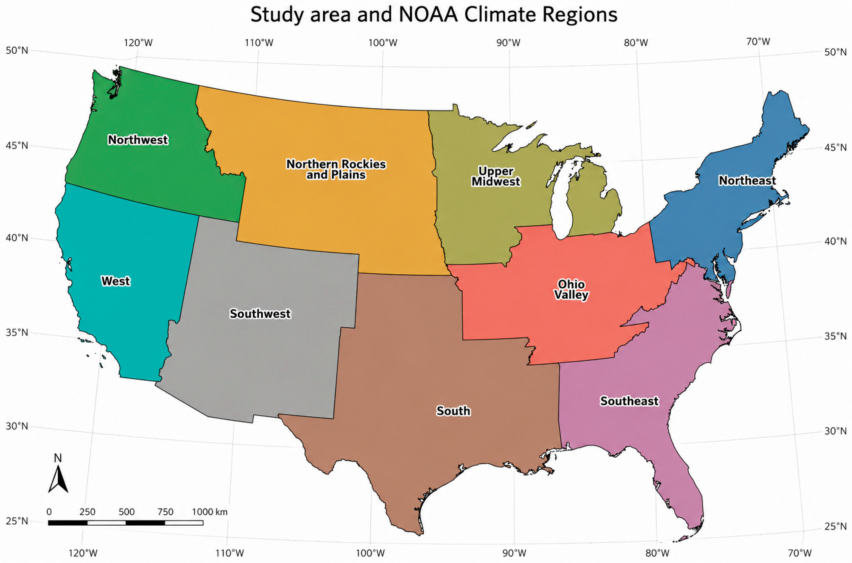
The study was conducted over the contiguous United States using the nine NOAA Climate Regions as the primary regional framework [19]. These regions provide a consistent spatial basis for evaluating large-scale precipitation changes across climatically distinct parts of the United States. The nine regions considered in this study were the Northeast, Upper Midwest, Ohio Valley, Southeast, Northern Rockies and Plains, South, Southwest, Northwest, and West. The regional framework used for aggregation is shown in Figure 1.

All analyses were performed at the regional scale rather than at the grid-cell scale. This choice was made to provide hydroclimatically interpretable regional summaries and to avoid direct pixel-level comparison between PRISM and NEX-GDDP-CMIP6, which differ in spatial resolution and data-generation methodology.

2.2. Observed Precipitation Data: PRISM

Observed precipitation changes were assessed using PRISM monthly precipitation data for 1941–2020. PRISM uses a physiographically informed interpolation framework designed to represent spatial climate patterns across the conterminous United States [14]. The observed period was divided into two 40-year subperiods: the early observed period, 1941–1980, and the recent observed period, 1981–2020.

Monthly PRISM precipitation grids were spatially aggregated over the NOAA Climate Regions to obtain regional monthly precipitation time series. For each region, the resulting time series contained 960 monthly values, corresponding to 80 years and 12 months per year. These regional monthly series formed the basis for the observed historical distributional analysis. Data sources and temporal coverage are summarized in Table S1.

2.3. Future Precipitation Projections: NEX-GDDP-CMIP6

Future precipitation changes were evaluated using NEX-GDDP-CMIP6 daily precipitation projections [16,17]. NEX-GDDP-CMIP6 is based on CMIP6 model output and was produced using a daily variant of the monthly Bias Correction/Spatial Disaggregation (BCSD) method. It provides bias-corrected, spatially downscaled daily climate projections under multiple SSP scenarios. CMIP6 model experiments follow the CMIP6 design framework [20], while the future scenarios follow the ScenarioMIP framework [21,22].

Four future SSP scenarios were evaluated: SSP1-2.6, SSP2-4.5, SSP3-7.0, and SSP5-8.5. The CMIP6 analysis used a selected five-model ensemble consisting of ACCESS-CM2, CanESM5, EC-Earth3, MRI-ESM2-0, and MIROC6. These models were retained because they provided complete NEX-GDDP-CMIP6 precipitation coverage for the historical experiment and all four SSP scenarios considered in this study, while also representing distinct modeling centers or model systems within the data-complete subset. The ensemble should be interpreted as a consistent selected-model set rather than as a probabilistic sample of the full CMIP6 archive. The selected models may not be fully independent because CMIP6 models can share components, development histories, or structural assumptions. Accordingly, ensemble medians were used as descriptive projected-change estimates, while selected-model spread was reported only to indicate model-to-model agreement or divergence. A supplementary model-coverage table lists the modeling centers and data-availability rationale for the selected models (Table S9). The selected models are therefore interpreted as a data-complete multi-model subset rather than as five statistically independent samples from a formal model population.

For each model, experiment, year, and region, monthly precipitation totals were summarized over the NOAA Climate Regions. Future changes were computed relative to each model’s own historical 1981–2014 regional climatology, rather than by directly comparing raw PRISM and raw CMIP6 values.

2.4. Regional Aggregation

For both PRISM and NEX-GDDP-CMIP6, precipitation fields were summarized over NOAA Climate Regions using spatial overlay between gridded precipitation data and regional polygons. For PRISM, regional means were computed from valid raster cells within each NOAA Climate Region after applying the regional mask in the raster-native grid. For NEX-GDDP-CMIP6, the NOAA polygons were represented in geographic coordinates (EPSG:4326), grid-cell centers were assigned to regions, and latitude-based cosine weights were used when calculating regional means. In all cases, missing or non-finite precipitation cells were excluded from regional averages.

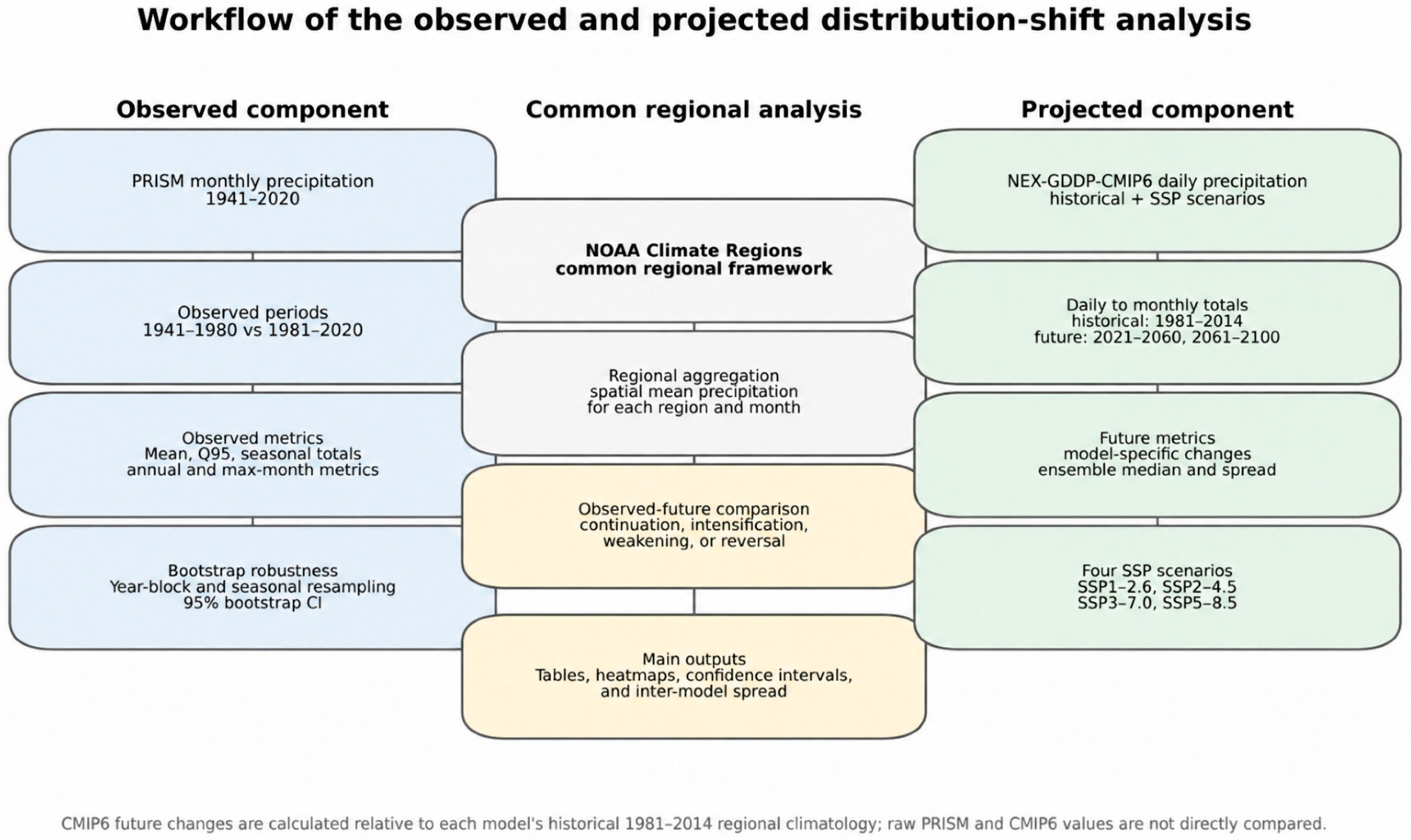
The same regional framework was used for the observed and future components of the study. All data processing, statistical analyses, and visualization were performed using author-developed Python scripts in Python 3.14.4 (64-bit). This provided a common spatial reporting basis while avoiding direct grid-cell-level comparison between PRISM and NEX-GDDP-CMIP6, which differ in spatial resolution, observational constraint, and data-generation methodology. The complete analysis workflow is summarized in Figure 2.

2.5. Distributional Shift Metrics

The analysis focused on changes in monthly precipitation distributions rather than only changes in annual or seasonal means. For each region and period, the following metrics were calculated: mean monthly precipitation, median monthly precipitation, coefficient of variation, skewness, Q95 monthly precipitation, Q99 monthly precipitation, seasonal precipitation totals, annual total precipitation, and annual maximum monthly precipitation. Here, Q95 and Q99 denote the 95th and 99th percentiles of monthly precipitation totals and are used as upper-tail monthly total diagnostics.

For PRISM, percentage changes were computed between the early observed period and the recent observed period. For CMIP6, percentage changes were computed between each model’s future period and its own historical reference period. CMIP6 ensemble results were summarized using the selected-model median, with the full selected-model range used as the main descriptive spread indicator. Supplementary percentile summaries are provided only as descriptive diagnostics and are not interpreted as formal probability intervals.

2.6. Seasonal and Annual Aggregation

Seasonal precipitation totals were calculated for DJF, MAM, JJA, and SON. Complete seasonal totals were retained for seasonal analysis. For DJF, December was assigned to the following season year, and incomplete winters at period boundaries were removed; therefore, complete DJF seasons were retained as 1942–1980 and 1982–2020 for the two PRISM-observed subperiods.

Annual total precipitation was calculated as the sum of monthly precipitation totals within each year. Annual maximum monthly precipitation was calculated as the maximum monthly precipitation value within each year. This metric was used to characterize high-month precipitation behavior at an annual scale.

2.7. Bootstrap Confidence Intervals for Observed Shifts

Bootstrap confidence intervals were used to evaluate the robustness of PRISM-based observed changes. For overall monthly distributional metrics, a year-block bootstrap approach was used to preserve the 12-month structure within each resampled year. For monthly climatology metrics, years were resampled within each calendar month. For seasonal metrics, complete seasonal totals were resampled.

Percentile-based 95% bootstrap confidence intervals were calculated using 5000 bootstrap replicates [23,24]. Observed changes were interpreted as robust only when the bootstrap confidence interval excluded zero. Intervals that included or touched zero were treated as not robust, even when the point estimate was positive. The percentile approach does not require symmetric bootstrap distributions, but it can be sensitive to serial dependence and block-length choices; this issue is evaluated using the supplementary 5-year block-bootstrap sensitivity test.

For clarity, robust means that the primary percentile-based 95% bootstrap confidence interval excluded zero, whereas not robust means that the interval included or touched zero. The term threshold-sensitive is used only as a qualitative qualifier for boundary cases or cases whose robust/not-robust classification changed under a supplementary sensitivity test; it is not a third statistical category and is not used to replace the robust/not robust decision rule.

2.8. CMIP6 Ensemble and Selected-Model Spread

For each CMIP6 model, future changes were calculated separately for each SSP scenario, region, metric, and future period. Model-specific percentage changes were then summarized across the five-model ensemble. The ensemble median was used as the primary projected change estimate.

Selected-model spread was represented primarily using the full min-max range across the five models, with ensemble medians used as descriptive central estimates. These spread estimates are indicators of model-to-model variation within the selected model set, not formal statistical confidence intervals or probabilistic uncertainty estimates [22,24]. This distinction is important because the selected ensemble was designed for consistent scenario comparison and is too small to support robust probabilistic inference about the full CMIP6 uncertainty space.

2.9. Method for Historical–Projected Directional Comparison

The historical-projected comparison was designed as a directional comparison, not as a model validation exercise. It evaluates whether PRISM-based historical shifts and CMIP6 late-century projected changes have similar signs, stronger projected magnitudes, weaker projected magnitudes, or divergent directions. The comparison focused on monthly mean precipitation and Q95 monthly precipitation. Observed PRISM changes were calculated between 19411980 and 1981–2020, while projected CMIP6 late-century changes were calculated for 2061–2100 relative to each model’s historical 1981–2014 reference period.

This comparison was not intended as a direct dataset-to-dataset validation, attribution analysis, or proof that observed changes will continue into the future. It was used only as a regional directional synthesis of historical PRISM shifts and scenario-based CMIP6 projected changes.

2.10. Supplementary Sensitivity Analyses

Three supplementary sensitivity analyses were conducted to evaluate whether key observed signals depended on methodological choices. First, the PRISM observed comparison was recalculated by replacing the 1981–2020 recent period with 1981–2014, matching the end year of the CMIP6 historical reference period. This test was used to evaluate whether the historical component of the directional comparison was sensitive to inclusion of 2015–2020.

Second, the bootstrap analysis was repeated using a 5-year block resampling design in addition to the primary 1-year-block bootstrap. This diagnostic test was used to assess whether robust/not-robust classifications were sensitive to multi-year precipitation variability. The sensitivity tests are reported in the Supplementary Materials and were used to qualify interpretation rather than replace the primary 40-year observed comparison.

Third, a leave-one-model-out sensitivity analysis was added for the CMIP6 SSP5-8.5 late-century monthly mean and Q95 changes. The test recalculated the selected-model median after omitting each model in turn and compared the resulting median range with the five-model median. This analysis was used descriptively to evaluate whether the reported CMIP6 medians were dominated by any single selected model; it does not estimate formal CMIP6 uncertainty, model genealogy, or effective sample size.

2.11. Historical CMIP6 Model-Performance Evaluation Against PRISM

To address historical model skill, the selected NEX-GDDP-CMIP6 historical simulations were evaluated against PRISM regional monthly precipitation for 1981–2014. Evaluation was conducted for each model and NOAA Climate Region using monthly time-series diagnostics and 12-month climatological-cycle diagnostics. The metrics included percent bias, mean absolute percent bias, RMSE, normalized RMSE, MAE, Pearson correlation, Kling–Gupta Efficiency, monthly climatology correlation, and monthly climatology Kling–Gupta Efficiency. The evaluation assesses whether the selected model subset reproduces regional monthly precipitation climatology sufficiently for screening-level interpretation; it does not convert the five-model subset into a probabilistic representation of the full CMIP6 uncertainty space. Taylor-diagram and monthly climatology validation figures are provided as supplementary diagnostics.

The historical evaluation was used as a suitability assessment rather than a model-selection filter, because the selected-model subset had already been defined by complete availability across the historical experiment and all four SSP scenarios. Therefore, performance metrics were used to contextualize the projected-change results, not to exclude or weight individual models.

Kling–Gupta Efficiency and Taylor-diagram diagnostics were used following Gupta et al. [25] and Taylor [26], respectively, and were added to address the reviewer request for historical model-performance evaluation.

2.12. Statistical Hypotheses, Effect Sizes, and FDR-Aware Testing

The analysis uses a hypothesis-testing structure to reduce reliance on descriptive percentage changes. H1 was evaluated using omnibus permutation tests of regional heterogeneity for observed mean and Q95 shifts, with pairwise post hoc diagnostics controlled within the H1 family when used. H2 was evaluated by bootstrapping the difference between upper-tail and mean changes (Delta Q95 minus Delta mean) and applying Benjamini–Hochberg false-discovery-rate correction across region-wise tests. H3 compared late-century SSP5-8.5 ensemble-median projected CMIP6 changes with an empirical PRISM historical-change envelope, defined as the 5th–95th percentile range of bootstrapped 40-year PRISM period-difference estimates. H4 evaluated whether historical model-performance metrics differed among the selected CMIP6 models. FDR correction was applied separately within each hypothesis family rather than across unrelated analyses.

Benjamini–Hochberg false-discovery-rate correction [27] was applied separately within each predefined hypothesis family, and Cliff’s delta [28] was used as a non-parametric effect-size diagnostic suitable for non-normal precipitation distributions.

2.13. Categorical Hydroclimatic Screening Matrix

A categorical Hydroclimatic Screening Matrix was developed a priori as a practitioner-facing classification tool rather than as a hydrologic risk index or predictive impact model. The matrix combines observed PRISM signal direction and robustness, projected late-century mean and Q95 change, seasonal redistribution, historical CMIP6 model skill, selected-model spread, and leave-one-model-out sensitivity. Categories were assigned using predefined if–then decision rules reported in Table S14a,b. Category A indicates an aligned planning-relevant precipitation signal; Category B indicates an emerging upper-tail concern; Category C indicates a seasonal-storage follow-up priority; Category E indicates directional uncertainty; and Category U indicates weak or unclassified screening evidence. Low model-performance or high-spread situations were retained as confidence qualifiers rather than being used as a primary hydrological category, so that category assignment did not overstate the certainty of projected magnitudes. When more than one rule was satisfied, the primary category was assigned according to the priority order defined in Table S14a,b.

3. Results

3.1. Observed Shifts in Monthly Precipitation Distributions

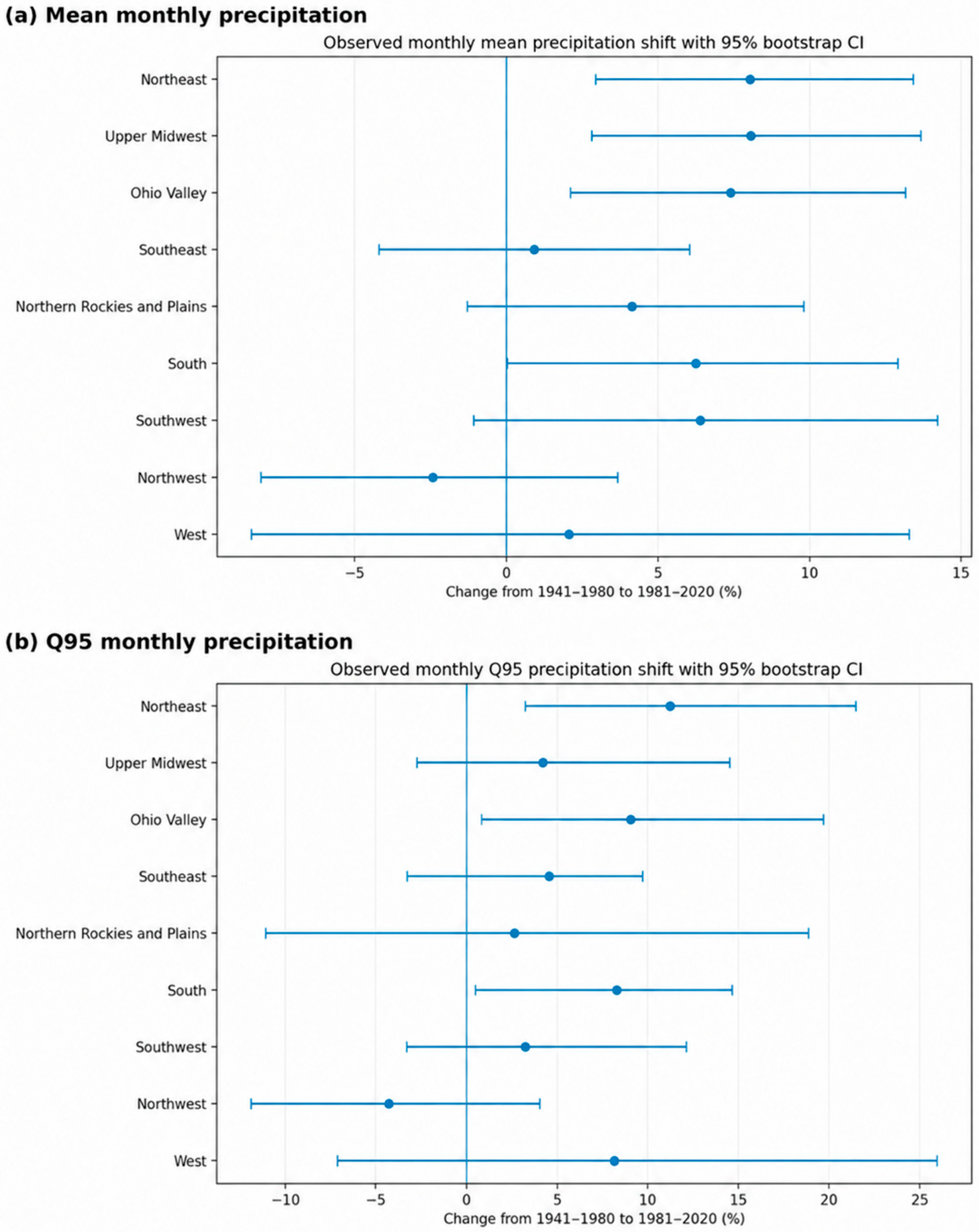
The PRISM-based observed analysis indicates that monthly precipitation distributions shifted upward in several U.S. climate regions between 1941–1980 and 1981–2020 (Figure 3;

Table 1. Observed PRISM monthly precipitation shift summary (1941–1980 to 1981–2020). Confidence intervals are percentile-based 95% bootstrap intervals.

Region	Mean Change (%)	Mean 95% CI (%)	Mean Bootstrap Result	Q95 Change (%)	Q95 95% CI (%)	Q95 Bootstrap Result	Interpretation
Northeast	8.0	[2.9, 13.4]	Robust	11.2	[3.2, 21.5]	Robust	Robust mean and Q95 wetting
Upper Midwest	8.1	[2.8, 13.7]	Robust	4.2	[−2.8, 14.5]	Not robust	Robust mean; Q95 not robust
Ohio Valley	7.4	[2.1, 13.1]	Robust	9.0	[0.8, 19.7]	Robust	Robust mean and Q95 wetting
Southeast	0.9	[−4.2, 6.0]	Not robust	4.6	[−3.3, 9.7]	Not robust	Weak observed signal
Northern Rockies and Plains	4.1	[−1.3, 9.8]	Not robust	2.7	[−11.1, 18.9]	Not robust	Weak observed signal
South	6.2	[0.0, 12.9]	Not robust	8.3	[0.5, 14.7]	Robust	Robust Q95; mean not robust (threshold-sensitive)
Southwest	6.4	[−1.1, 14.2]	Not robust	3.2	[−3.3, 12.1]	Not robust	Weak observed signal
Northwest	−2.4	[−8.1, 3.7]	Not robust	−4.3	[−11.9, 4.0]	Not robust	Negative but not robust
West	2.1	[−8.4, 13.3]	Not robust	8.1	[−7.1, 26.0]	Not robust	Weak observed signal

). Mean monthly precipitation increased robustly in the Northeast, Upper Midwest, and Ohio Valley. The South also showed a positive mean change of approximately 6.2%, but its bootstrap interval touched zero and is therefore classified as not robust; because the lower bound is near the decision threshold, it is described qualitatively as threshold-sensitive. Mean monthly precipitation increased by approximately 8.0% in the Northeast, 8.1% in the Upper Midwest, and 7.4% in the Ohio Valley, with bootstrap confidence intervals excluding zero. Full observed monthly metrics, monthly climatology shifts, annual diagnostics, and bootstrap diagnostics are provided in Table S2 and Figures S1–S3.

Upper-tail monthly precipitation also increased in selected regions. The Q95 of monthly precipitation increased robustly by approximately 11.2% in the Northeast and 8.3% in the South. The Ohio Valley Q95 increase was positive in the primary analysis, but its bootstrap classification was sensitive to the alternative 5-year block-bootstrap test. These regions therefore exhibited changes not only in central tendency but also in the upper tail of the monthly precipitation distribution. In contrast, some regions showed positive point estimates that were not robust under the bootstrap intervals, indicating greater uncertainty in the magnitude of observed changes.

The Northwest showed a different observed behavior, with negative point estimates for both mean monthly precipitation and Q95 precipitation. However, the broader regional pattern indicates that observed precipitation changes over the last 80 years were spatially heterogeneous, with the strongest and most robust wetting signals concentrated in central and eastern U.S. climate regions.

3.2. Observed Seasonal Redistribution

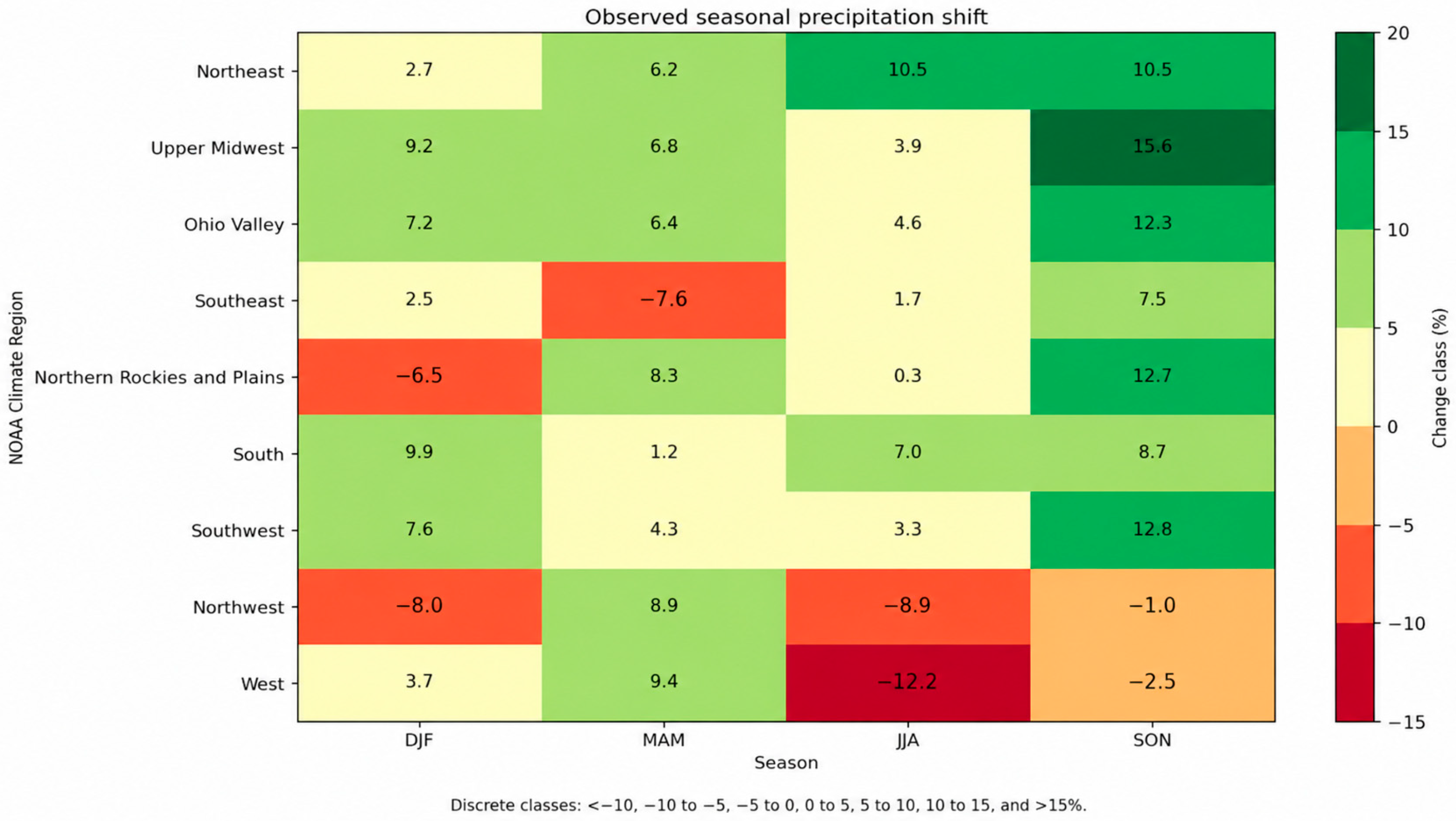
Seasonal aggregation revealed that observed precipitation changes were not uniform throughout the year (Figure 4; Table S3). Autumn precipitation showed the most spatially consistent positive shift across several regions. SON precipitation showed bootstrap-supported increases in the Upper Midwest, Ohio Valley, and Northeast, with changes of approximately 15.6%, 12.3%, and 10.5%, respectively. The Northeast also showed a robust JJA increase, while the Northern Rockies and Plains exhibited a bootstrap-supported MAM increase.

These results suggest that the observed historical wetting signal was partly associated with seasonal redistribution rather than uniform increases across all months. In several central and eastern regions, increases in autumn precipitation contributed strongly to the overall observed distributional shift. In western and northwestern regions, seasonal changes were more complex, with negative point estimates in some seasons but wider bootstrap uncertainty.

3.3. Projected Future Shifts in Monthly Mean Precipitation

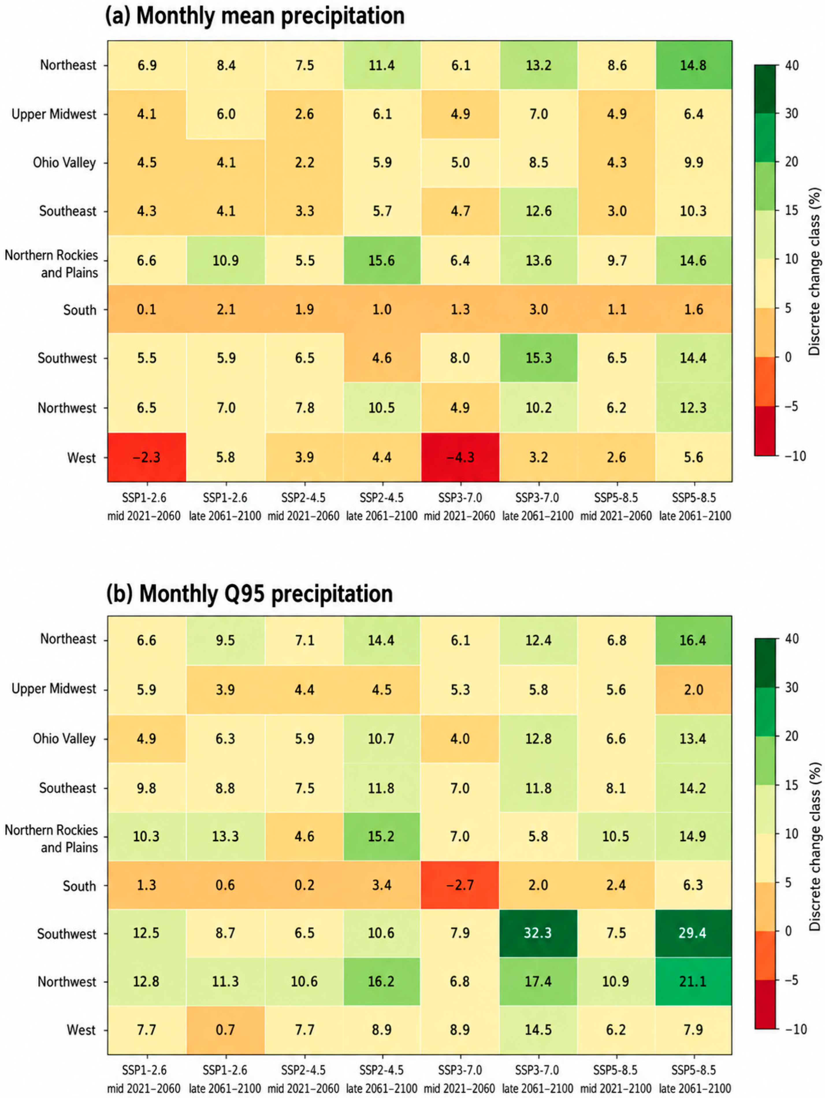
The CMIP6 future analysis indicates broad projected increases in monthly mean precipitation across most U.S. climate regions, with larger changes under higher-emission scenarios and during the late-century period (Figure 5;

Table 2. CMIP6 late-century SSP5-8.5 projected precipitation shift summary (1981–2014 to 2061–2100). Values are ensemble medians relative to each model’s historical reference period.

Region	n Models	Monthly Mean Change (%)	Monthly Q95 Change (%)	Annual Total Mean Change (%)	Annual Max-Month Q95 Change (%)
Northeast	5	14.8	16.4	14.8	13.7
Upper Midwest	5	6.4	2.0	6.4	9.8
Ohio Valley	5	9.9	13.4	9.9	9.2
Southeast	5	10.3	14.2	10.3	20.6
Northern Rockies and Plains	5	14.6	14.9	14.6	9.4
South	5	1.6	6.3	1.6	3.7
Southwest	5	14.4	29.4	14.4	28.9
Northwest	5	12.3	21.1	12.3	16.6
West	5	5.6	7.9	5.6	23.8

). Under SSP5-8.5 during 2061–2100, ensemble-median mean monthly precipitation increased most strongly in the Northeast, Northern Rockies and Plains, Southwest, Northwest, Southeast, and Ohio Valley. Full scenario-period monthly summaries and monthly climatology diagnostics are provided in Table S4 and Figure S4.

The largest late-century SSP5-8.5 mean monthly increases were approximately 14.8% in the Northeast, 14.6% in the Northern Rockies and Plains, 14.4% in the Southwest, and 12.3% in the Northwest. The Southeast and Ohio Valley also showed positive changes of approximately 10.3% and 9.9%, respectively. In contrast, the South showed a comparatively weak late-century SSP5-8.5 mean increase of approximately 1.6%, indicating that projected future wetting is not spatially uniform.

Scenario dependence was evident across the CMIP6 results. Projected changes were generally smaller under SSP1-2.6 and larger under SSP5-8.5, especially during 2061–2100. This indicates that monthly precipitation distribution shifts are expected to intensify under higher-emission pathways, although the magnitude and regional pattern of change vary substantially. Because the analysis used relative changes within each model, these scenario differences represent projected distributional responses rather than direct comparisons between raw PRISM and CMIP6 precipitation amounts.

3.4. Projected Upper-Tail Intensification

Projected changes in the upper tail of the monthly precipitation distribution were generally stronger than changes in the mean in several regions. Under SSP5-8.5 during 2061–2100, the Q95 of monthly precipitation increased by approximately 29.4% in the Southwest, 21.1% in the Northwest, 16.4% in the Northeast, 14.9% in the Northern Rockies and Plains, 14.2% in the Southeast, and 13.4% in the Ohio Valley. These Q95 values describe upper-tail monthly totals in the downscaled product and should not be interpreted as daily event extremes or direct flood-risk estimates.

These results indicate that future precipitation change is not limited to shifts in central tendency. In several regions, high-month precipitation behavior is projected to intensify more strongly than mean monthly precipitation. This pattern is particularly evident in the Southwest, where the projected late-century SSP5-8.5 Q95 increase is substantially larger than the corresponding mean increase.

Annual maximum monthly precipitation results were generally consistent with the monthly upper-tail findings. Under late-century SSP5-8.5, the upper tail of annual maximum monthly precipitation intensified particularly in the Southwest, West, Southeast, Northwest, and Northeast. These findings should be interpreted as screening-level indicators of high-month precipitation behavior rather than direct estimates of flood risk or runoff response.

3.5. Projected Seasonal Redistribution

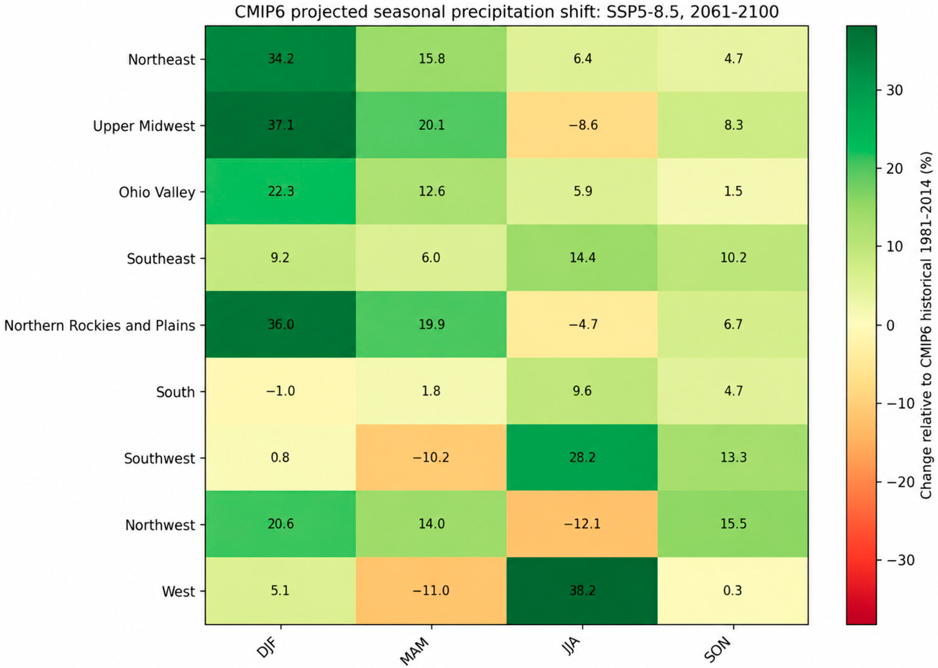
Future precipitation changes showed a strong seasonal structure (Figure 6). Under SSP5-8.5 during 2061–2100, winter precipitation increased markedly in northern and interior regions. DJF precipitation increased by approximately 37.1% in the Upper Midwest, 36.0% in the Northern Rockies and Plains, 34.2% in the Northeast, 22.3% in the Ohio Valley, and 20.6% in the Northwest. Detailed seasonal values are reported in Table S5, and projected annual total and annual maximum monthly precipitation diagnostics are provided in Figure S5.

Western and southwestern regions showed more complex seasonal redistribution. The West and Southwest exhibited large projected summer increases under SSP5-8.5 during 2061–2100, while some spring changes were negative. These results indicate that projected future precipitation shifts involve not only regional wetting but also redistribution of precipitation across seasons.

The seasonal results are important because annual or overall monthly statistics can mask changes in the timing of precipitation. In several regions, projected increases are concentrated in particular seasons, suggesting that further hydrologic impact modeling may be needed to evaluate how seasonal precipitation redistribution interacts with snow-season processes, soil moisture, evapotranspiration, and runoff generation.

3.6. Supplementary Sensitivity Checks for the Observed Component

The PRISM reference-period sensitivity test showed that the sign of the mean change was unchanged in eight of nine regions when the recent observed period was limited to 1981–2014 rather than 1981–2020 (Figure S6a,b; Table S7). The only mean-direction difference occurred in the Southeast, where both the primary and sensitivity estimates were non-robust. For Q95, all regions retained the same change direction under the alternative observed reference period.

The 5-year block-bootstrap sensitivity test indicated that most robust/not-robust classifications were unchanged, but three of eighteen region-metric pairs changed classification (Figure S7; Table S8). Ohio Valley Q95 changed from robust to not robust under the longer block design, whereas Southwest mean and Southwest Q95 changed from not robust to robust. The South mean signal remained not robust under the conservative primary classification and the 5-year block design, but its confidence interval boundary was close to zero, illustrating the sensitivity of boundary cases. Thus, classification changes occurred in both directions rather than systematically weakening the observed signals. The final column of Table S8 identifies the direction of classification changes and marks boundary-sensitive cases.

Such threshold sensitivity is plausible for regional precipitation because multi-year wet and dry episodes, teleconnection-related variability, and low-frequency ocean-atmosphere variability can affect the effective number of independent years represented in a resampling experiment. The sensitivity analysis therefore supports the broad directional stability of the main observed patterns while showing that marginal robust/not-robust labels should not be overinterpreted.

3.7. Historical-Projected Directional Comparison

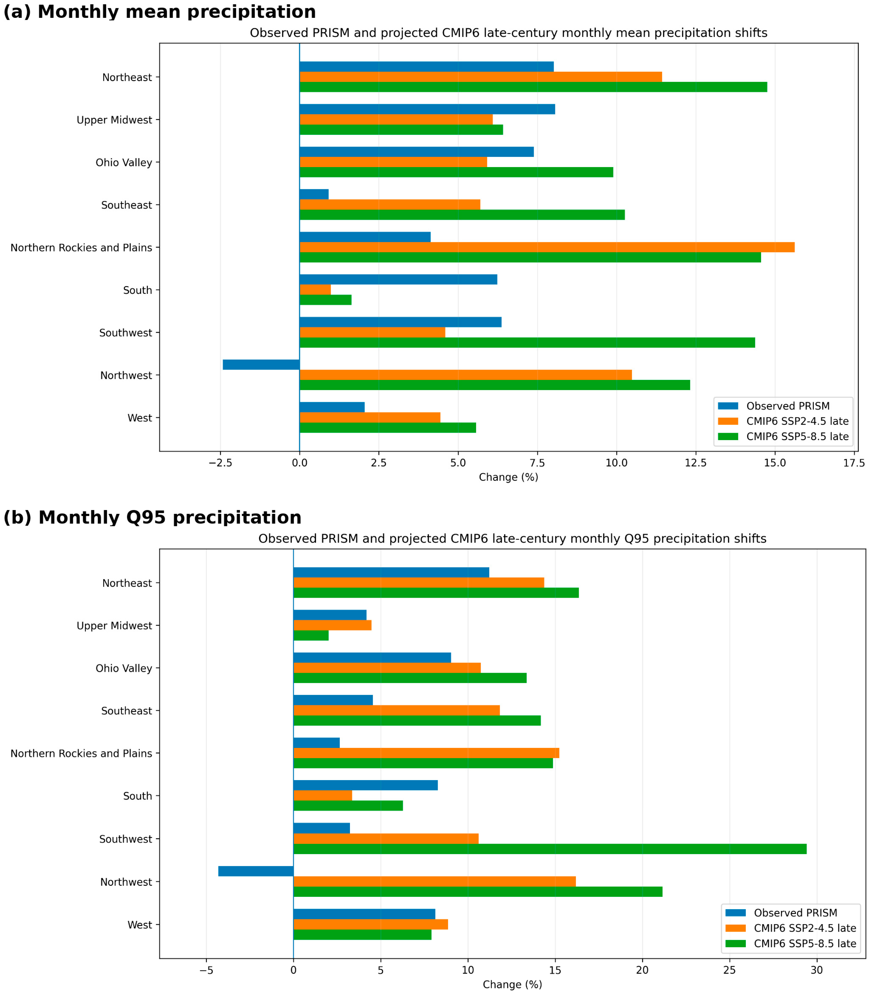
The directional comparison between PRISM observed shifts and CMIP6 projected late-century shifts indicates both regional alignment and regional divergence (Figure 7;

Table 3. Historical-projected directional comparison summary. PRISM historical shifts are compared directionally with CMIP6 late-century SSP2-4.5 and SSP5-8.5 projections; the comparison is not a direct validation.

Region	Observed Mean (%)	SSP2-4.5 Late Mean (%)	SSP5-8.5 Late Mean (%)	Observed Q95 (%)	SSP2-4.5 Late Q95 (%)	SSP5-8.5 Late Q95 (%)	Interpretation
Northeast	8.0	11.4	14.8	11.2	14.4	16.4	Aligned positive; projected intensification
Upper Midwest	8.1	6.1	6.4	4.2	4.5	2.0	Aligned mean; weak projected Q95
Ohio Valley	7.4	5.9	9.9	9.0	10.7	13.4	Aligned positive signal
Southeast	0.9	5.7	10.3	4.6	11.8	14.2	Projected wetting; weak historical signal
Northern Rockies and Plains	4.1	15.6	14.6	2.7	15.2	14.9	Projected intensification; weak historical signal
South	6.2	1.0	1.6	8.3	3.4	6.3	Observed Q95 wetting; weak projected mean
Southwest	6.4	4.6	14.4	3.2	10.6	29.4	Projected intensification; weak historical signal
Northwest	−2.4	10.5	12.3	−4.3	16.2	21.1	Divergent historical and projected directions
West	2.1	4.4	5.6	8.1	8.9	7.9	Weak historical; modest projected wetting

). The Northeast and Ohio Valley show aligned positive signals across the observed and future analyses. In these regions, observed PRISM increases in mean and upper-tail monthly precipitation have the same direction as projected CMIP6 increases under SSP2-4.5 and SSP5-8.5.

Other regions show more divergent historical-projected behavior. The Northwest exhibited negative observed point estimates but positive projected future changes, indicating divergent historical and projected directions rather than a validated reversal. The Southwest showed modest observed changes but much stronger projected future increases, especially in upper-tail monthly precipitation under SSP5-8.5. The South showed robust observed Q95 increases but comparatively weak projected future mean changes, indicating that future change may not simply continue the observed historical pattern.

These results show that observed historical changes should not be interpreted as direct analogs of future projected changes in all regions. Instead, the historical and projected signals should be evaluated together to identify regions where directions align, where projected changes intensify, and where future scenario-based changes diverge from recent historical behavior.

3.8. Selected-Model Spread and Leave-One-Model-Out Sensitivity in CMIP6 Projections

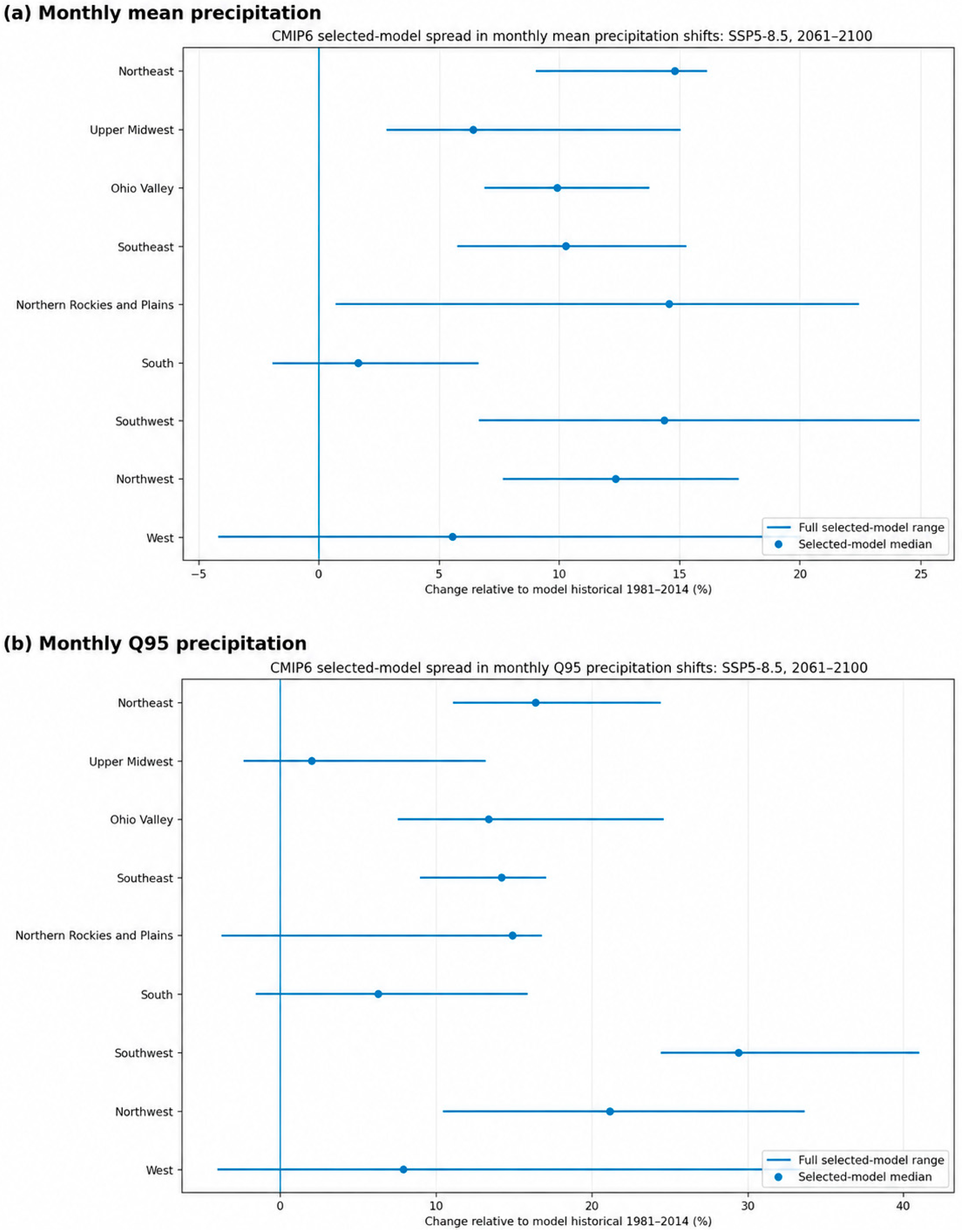
Selected-model spread analysis shows that projected changes vary substantially across regions and metrics (Figure 8; Table S6). Mean monthly precipitation shifts generally show clearer positive ensemble-median signals than upper-tail shifts. However, some regions exhibit wide selected-model ranges, indicating greater model-to-model variation in projected magnitudes.

Under SSP5-8.5 during 2061–2100, the Northeast shows a relatively consistent positive mean precipitation signal across the selected model ensemble. In contrast, regions such as the West, Southwest, and Northern Rockies and Plains exhibit wider selected-model ranges, especially for Q95 precipitation. This indicates that upper-tail precipitation projections have greater model-to-model variation than mean precipitation projections, which is expected because upper-tail metrics are more sensitive to model structure, sample variability, and downscaling behavior.

The selected-model spread results should be interpreted as descriptive model-to-model variation rather than formal statistical confidence intervals. They provide useful information about whether the selected models point in similar or divergent directions, but they do not quantify internal variability, model structural dependence, or the full CMIP6 uncertainty space. Regions with wider ranges therefore require more cautious interpretation.

The leave-one-model-out sensitivity analysis further showed that the late-century SSP5-8.5 selected-model medians were not controlled by a single model for most region-metric pairs (Figure S8a,b; Table S10). Of the 18 monthly mean and Q95 region-metric pairs, 11 had a maximum leave-one-model-out shift smaller than 3 percentage points, six had moderate sensitivity between 3 and 5 percentage points, and one pair, Northern Rockies and Plains Q95, had high sensitivity of at least 5 percentage points. All leave-one-model-out median ranges remained positive, but the larger sensitivity in selected western and northern regions reinforces the need to treat upper-tail projected magnitudes as descriptive rather than probabilistic.

3.9. Historical CMIP6 Model Performance Against PRISM

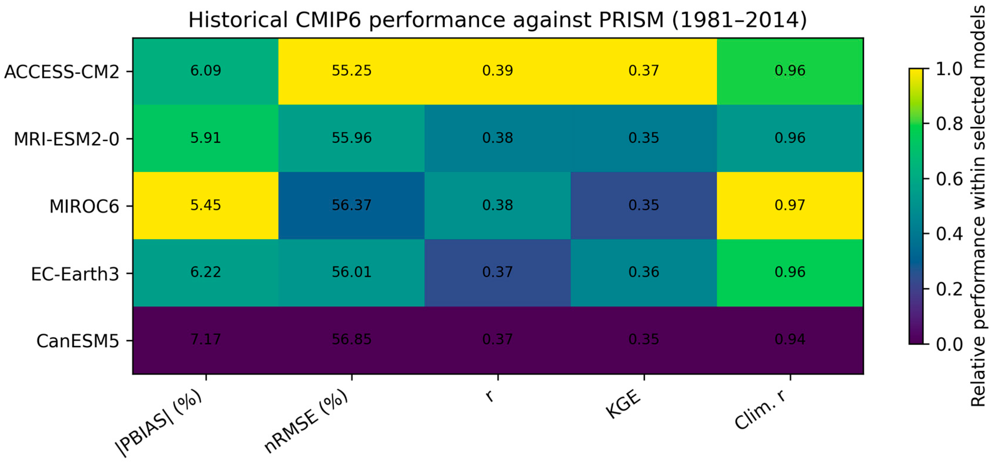
The added historical evaluation showed that the selected five NEX-GDDP-CMIP6 models reproduced the regional monthly climatological cycle substantially better than they reproduced month-to-month anomalies. Across the nine NOAA Climate Regions, monthly climatology correlations ranged from 0.943 to 0.969 and monthly climatology KGE ranged from 0.834 to 0.886 (

Table 4. Historical CMIP6 model-performance summary against PRISM for 1981–2014. Values are averages across the nine NOAA Climate Regions.

Model	Mean Abs. Bias (%)	RMSE (mm)	r	KGE	Climatology r	Climatology KGE	Rank
ACCESS-CM2	6.088	35.383	0.388	0.366	0.963	0.870	1
MRI-ESM2-0	5.910	35.878	0.376	0.354	0.957	0.886	2
MIROC6	5.449	35.907	0.377	0.351	0.969	0.877	3
EC-Earth3	6.216	35.936	0.372	0.355	0.963	0.873	4
CanESM5	7.172	36.226	0.366	0.346	0.943	0.834	5

; Figure 9). Mean absolute percent bias ranged from approximately 5.4% to 7.2%. In contrast, raw monthly time-series correlations were lower, approximately 0.37–0.39, and monthly time-series KGE values were approximately 0.35–0.37. These results support the use of the selected ensemble for screening-level climatological and relative-change diagnostics, while reinforcing the need for caution in interpreting year-to-year variability or probabilistic uncertainty.

3.10. Hypothesis-Testing and FDR-Aware Statistical Diagnostics

The hypothesis-testing results indicate that the analysis is not limited to descriptive percentage changes (

Table 5. Summary of formal hypotheses, statistical tests, and FDR-aware interpretations used in this study.

Hypothesis	Question	Primary Test	Metric/Family	Main Result	Interpretation
H1	Observed shifts differ among NOAA Climate Regions	omnibus regional heterogeneity permutation	mean	p = 0.294	regional heterogeneity not supported at 0.05
H1	Observed shifts differ among NOAA Climate Regions	omnibus regional heterogeneity permutation	q95	p = 0.189	regional heterogeneity not supported at 0.05
H2	Upper-tail changes exceed mean changes	bootstrap ΔQ95−ΔMean with BH-FDR	region-wise amplification tests	0/9 regions FDR-significant	see Table S12 for regional details
H3	Late-century projections fall outside empirical historical-change envelope	comparison with PRISM bootstrapped 40-year change envelope	mean and Q95, region-wise	14/18 region-metric pairs outside envelope	screening diagnostic, not attribution or validation
H4	Historical performance metrics differ among selected CMIP6 models	permutation test of between-model performance differences	KGE, nRMSE, climatology correlation	0/3 model-performance tests FDR-significant	see Table 4 and Table S11 for model ranking/performance

). H1 omnibus regional-heterogeneity tests were not significant for observed mean or Q95 shifts. H2 upper-tail amplification tests showed no FDR-significant regional cases for Delta Q95 minus Delta mean. H3 provided the strongest envelope-based screening comparison: late-century SSP5-8.5 projected CMIP6 changes fell outside the empirical PRISM historical-change envelope in 14 of 18 region-metric pairs. This result is interpreted as a screening diagnostic rather than attribution, validation, or proof of forced response. H4 indicated that between-model differences in selected historical performance metrics were not FDR-significant, although descriptive model ranking and regional skill diagnostics remain informative.

The purpose of these tests was not to maximize the number of statistically significant findings, but to evaluate whether the descriptive interpretations remained statistically defensible. Accordingly, the non-significant H1, H2, and H4 results are informative: they indicate that regional differences, upper-tail amplification, and model-performance contrasts should not be overinterpreted as formally significant in this dataset. The H3 envelope comparison provides complementary screening evidence by showing that most late-century SSP5-8.5 projected mean and Q95 changes exceed the empirical PRISM historical-change envelope; this supports the use of the results as screening diagnostics rather than deterministic hydrological-impact estimates.

3.11. Hydroclimatic Screening Matrix Classification

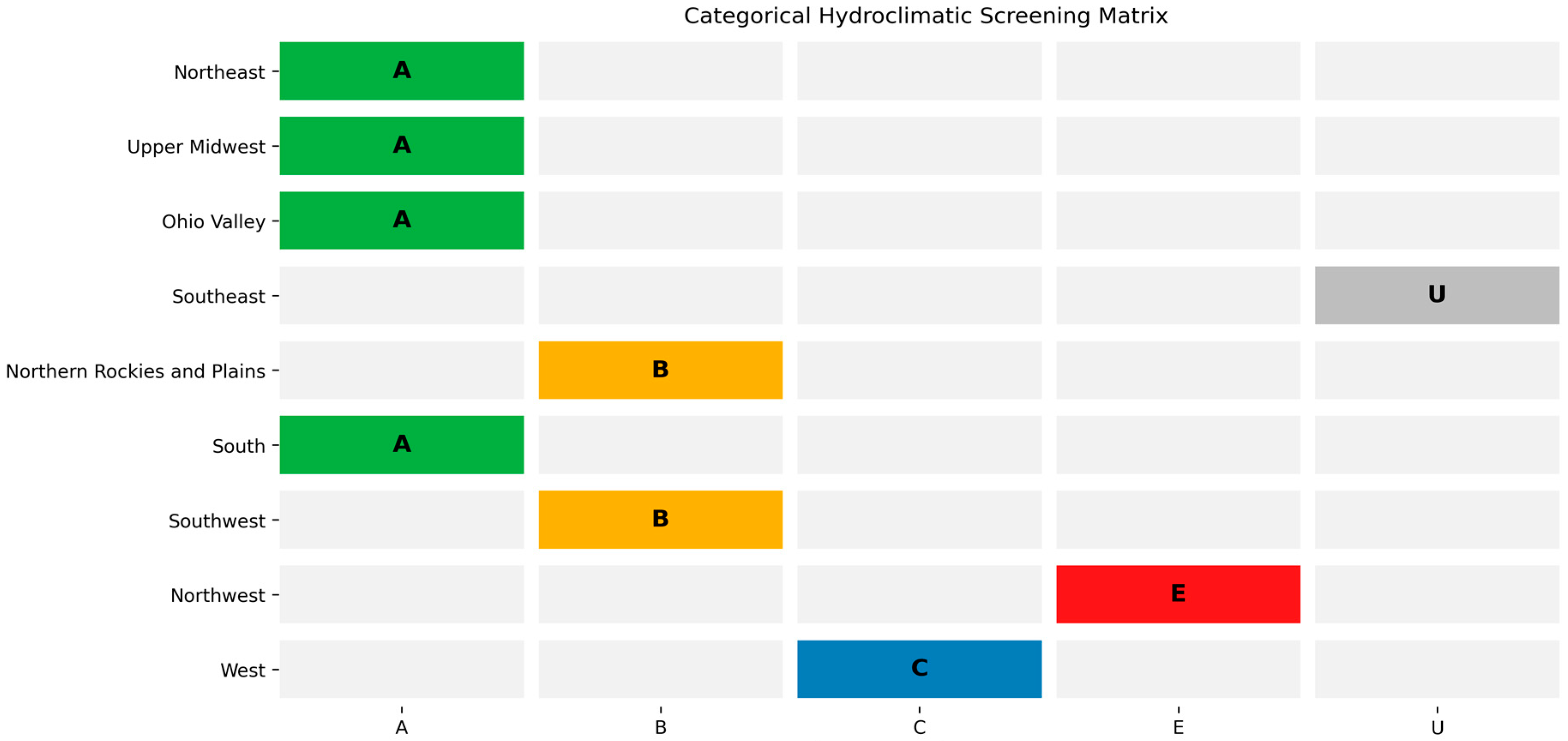
The categorical Hydroclimatic Screening Matrix translated observed, projected, seasonal, and model-evaluation diagnostics into regional follow-up categories (

Table 6. Categorical Hydroclimatic Screening Matrix classification. Projected basis uses late-century SSP5-8.5 summary values from the existing directional-comparison results; confidence qualifiers are reported separately to avoid overstating magnitude certainty.

Region	Category	Primary Interpretation	Observed Basis	SSP5-8.5 Late Basis	Qualifier
Northeast	A	Aligned planning-relevant precipitation signal	mean 8.0%, Q95 11.2%	mean 14.8%, Q95 16.4%	confidence qualifier reported separately
Upper Midwest	A	Aligned planning-relevant precipitation signal	mean 8.1%, Q95 4.2%	mean 6.4%, Q95 2.0%	confidence qualifier reported separately
Ohio Valley	A	Aligned planning-relevant precipitation signal	mean 7.4%, Q95 9.0%	mean 9.9%, Q95 13.4%	confidence qualifier reported separately
Southeast	U	Unclassified/weak screening signal	mean 0.9%, Q95 4.6%	mean 10.3%, Q95 14.2%	confidence qualifier reported separately
Northern Rockies and Plains	B	Emerging upper-tail concern	mean 4.1%, Q95 2.7%	mean 14.6%, Q95 14.9%	confidence qualifier reported separately
South	A	Aligned planning-relevant precipitation signal	mean 6.2%, Q95 8.3%	mean 1.6%, Q95 6.3%	confidence qualifier reported separately
Southwest	B	Emerging upper-tail concern	mean 6.4%, Q95 3.2%	mean 14.4%, Q95 29.4%	confidence qualifier reported separately
Northwest	E	Directional uncertainty; avoid trend-continuation assumptions	mean −2.4%, Q95 −4.3%	mean 12.3%, Q95 21.1%	confidence qualifier reported separately
West	C	Seasonal-storage follow-up priority	mean 2.1%, Q95 8.1%	mean 5.6%, Q95 7.9%	confidence qualifier reported separately

; Figure 10). The Northeast, Upper Midwest, Ohio Valley, and South were classified as Category A, indicating aligned planning-relevant precipitation signals. The Northern Rockies and Plains and Southwest were classified as Category B, indicating emerging upper-tail concerns. The West was classified as Category C because seasonal redistribution was the dominant screening feature. The Northwest was classified as Category E because observed and projected directions diverged. The Southeast was classified as U because it lacked a strong primary screening pattern under the defined rules. As a worked example, the Southwest had weak or non-robust historical signals but strong projected late-century upper-tail change under SSP5-8.5, leading to an emerging upper-tail concern classification while retaining a confidence qualifier for magnitude interpretation. Category assignments were generated from the predefined Table S14a,b rules rather than from post hoc interpretation of individual regions.

4. Discussion

4.1. Regional Heterogeneity of Observed Monthly Precipitation Shifts

The PRISM-based results demonstrate that observed changes in monthly precipitation distributions across U.S. climate regions are regionally heterogeneous. This heterogeneity is physically plausible because precipitation over the United States is shaped by regional moisture transport, synoptic storm tracks, convective activity, topography, and seasonally varying circulation patterns [5,6,18,29,30]. The stronger observed wetting in the Northeast, Upper Midwest, and Ohio Valley is consistent with the broader tendency for humid central and eastern regions to show increasing precipitation and heavy-precipitation behavior, whereas western regions are more strongly affected by seasonal redistribution and multidecadal variability.

The Northeast and Ohio Valley are regions where frontal systems, extratropical cyclones, and moisture convergence can contribute to both frequent precipitation and high monthly totals. In such settings, an increase in atmospheric moisture availability can affect not only average monthly precipitation but also the upper part of the monthly distribution when favorable dynamical conditions occur. This provides a process-based context for the observed alignment between mean and Q95 increases in these regions.

In contrast, western and northwestern regions showed more complex behavior. The Northwest exhibited negative observed point estimates, while the West showed limited mean change and non-robust positive upper-tail point estimates. These patterns may be influenced by precipitation seasonality, atmospheric-river variability, snow-season processes, and low-frequency Pacific variability. Therefore, the western results are better interpreted as period-to-period distributional shifts than as simple monotonic trends.

4.2. Importance of Seasonal Redistribution

The observed seasonal results indicate that precipitation shifts were strongly influenced by seasonal redistribution. Autumn precipitation increases in the Upper Midwest, Ohio Valley, and Northeast suggest that the historical wetting signal was not uniform across all months. This distinction matters because identical annual precipitation changes can have different water-resource implications depending on whether they occur during the growing season, recharge season, or snow-influenced part of the year [6,12,31].

The future CMIP6 results also showed strong seasonal structure, especially under SSP5-8.5 during 2061–2100. DJF increases in northern and interior regions may be relevant to snow-rain partitioning, seasonal storage, soil-moisture recharge, and melt timing, while western and southwestern regions showed more complex redistribution.

These seasonal diagnostics identify where process-based follow-up analyses would be most relevant. They do not simulate hydrological pathways directly, but they help prioritize where basin-scale hydrologic or land-surface modeling could evaluate runoff, recharge, snowpack, or storage responses.

4.3. Upper-Tail Precipitation Metrics and Downscaling Considerations

Upper-tail monthly precipitation changes were often larger than mean changes, particularly in projected late-century results. This pattern is consistent with the broader understanding that high-end precipitation can intensify under warming conditions when increased moisture availability coincides with favorable circulation and triggering conditions [7,8,9,10,32,33,34,35]. However, the Q95 and Q99 metrics used here are upper-tail diagnostics of monthly totals, not daily event extremes.

This distinction is central to interpretation. Monthly Q95 increases indicate wetter high-precipitation months, but they do not directly quantify storm intensity, flood peaks, design rainfall, runoff coefficients, or reservoir inflow extremes. Because NEX-GDDP-CMIP6 is bias-corrected and spatially downscaled using a BCSD-based approach [16,17], projected upper-tail metrics are treated as downscaled monthly total diagnostics rather than direct hydrological-impact estimates.

4.4. Historical-Projected Alignment and Divergence

The historical-projected directional comparison was retained as a synthesis rather than a validation or attribution exercise. PRISM-based historical shifts reflect observed gridded precipitation changes over 1941–2020, including forced change, internal variability, and gridded-data characteristics, whereas CMIP6 future shifts represent scenario-based model responses relative to each model’s historical baseline.

Alignment between observed and projected changes therefore indicates directional coherence, while divergence indicates that recent historical behavior should not be assumed to continue directly into the future. The Northeast and Ohio Valley showed aligned positive signals, whereas the Northwest and Southwest illustrated divergent or intensifying projected behavior. These differences support the screening framing while keeping observational and projection baselines conceptually separate.

4.5. Scenario Dependence of Future Distributional Shifts

The CMIP6 results show that projected precipitation changes are scenario dependent, with stronger late-century changes generally occurring under SSP5-8.5. This scenario dependence is consistent with the CMIP6/ScenarioMIP design, where future forcing pathways represent different socioeconomic and emissions trajectories [4,21,22]. The scenario differences are most appropriately interpreted as relative distributional responses within each model rather than as comparisons of raw precipitation magnitudes across datasets.

However, scenario dependence is not uniform across all regions. Some regions show positive projected changes across scenarios, while others show larger differences between lower- and higher-emission pathways. This regional variation indicates that precipitation distribution changes are shaped by both large-scale forcing and regional circulation dynamics. The results are therefore useful for identifying scenario-sensitive regions, but they do not assign probabilities to individual SSP pathways.

4.6. Selected-Model Spread in CMIP6 Projections

Selected-model spread was larger for upper-tail metrics than for mean precipitation metrics. This is expected because upper-tail and extreme-value metrics are more sensitive to model differences, internal variability, sample size, and downscaling behavior [24,36,37,38]. Therefore, upper-tail projections should be interpreted with greater caution than mean changes, especially in regions where the selected-model range is wide.

The spread analysis indicates that some projected changes are more consistent across the selected models than others. For example, the Northeast showed a relatively consistent positive late-century mean precipitation signal, while regions such as the West, Southwest, and Northern Rockies and Plains showed wider ranges for some metrics. Because only five models were used, these ranges should not be treated as robust percentiles of the CMIP6 population. They are descriptive summaries of the selected ensemble.

It is important to emphasize that the selected-model spread shown in this study does not represent a formal statistical confidence interval and does not separate model structural uncertainty from internal variability. The leave-one-model-out test showed that 11 of 18 monthly mean and Q95 region-metric pairs had a maximum median shift below 3 percentage points, six had moderate shifts of 3–5 percentage points, and only one had a shift of at least 5 percentage points. This reduces the risk that the SSP5-8.5 late-century medians are dominated by a single selected model, but it does not replace a larger ensemble, model genealogy analysis, or initial-condition ensemble assessment. Future work may expand the model set, evaluate model dependence more explicitly, and test whether performance-based weighting changes the regional conclusions.

The non-significant tests also help constrain the revised claims. They show that the manuscript should emphasize robust observed changes, projected changes outside historical-change envelopes, and screening classifications, rather than claiming that all regions differ significantly or that all upper-tail changes exceed mean changes. This conservative interpretation strengthens the analysis by limiting claims to statistically defensible findings.

The historical model evaluation also supports a measured interpretation of the projections. Monthly climatology skill was relatively strong, whereas month-to-month time-series skill was lower. This result is consistent with the use of CMIP6 output for regional climatological screening, but it cautions against interpreting the selected models as precise predictors of individual monthly anomalies. The evaluation therefore contextualizes, rather than guarantees, the reliability of future distributional shifts.

4.7. Categorical Hydroclimatic Screening for Water-Resource Follow-Up Prioritization

The Hydroclimatic Screening Matrix provides a more direct water-resource contribution while remaining within the precipitation-based scope of the study. The matrix was developed a priori from predefined if–then rules reported in Table S14a,b and is intended as a practitioner-facing classification tool for follow-up prioritization, not as a hydrologic risk index or predictive impact model.

The matrix organizes observed robustness, projected upper-tail and seasonal changes, model-evaluation results, selected-model spread, and directional agreement into categories that identify where basin-scale hydrologic modeling may be prioritized. When more than one rule is satisfied, the primary category follows the priority order Table S14a,b, while model-performance and selected-model spread are retained as confidence qualifiers rather than overriding the primary hydroclimatic category.

For example, the Southwest was classified as an emerging upper-tail concern because observed historical signals were relatively weak but projected late-century Q95 increases were large. This classification does not imply a quantified flood or runoff impact; rather, it identifies a region where daily event analysis, soil-moisture assessment, and basin-scale hydrologic modeling would be a logical next step. This worked example illustrates how the matrix translates precipitation diagnostics into follow-up priorities without overstating hydrological consequences.

The South was retained as an aligned planning-relevant signal because the matrix prioritizes the combined observed upper-tail signal and positive projected direction; however, its weak projected mean change and non-robust observed mean are explicitly reflected in the confidence qualifier and in Table 6 rather than treated as a direct hydrologic-impact result.

4.8. Implications for Hydroclimatic Assessment and Water-Resource Planning

The results support the use of monthly precipitation distributions as a regional screening layer for water-resource assessment. Rather than relying only on annual mean precipitation, planners can use distributional, upper-tail, seasonal, and historical-projected diagnostics to identify regions where follow-up assessment may be warranted.

The findings are most useful for prioritizing dedicated hydrologic analyses of streamflow response, soil-moisture storage, snow-rain partitioning, reservoir operation, drought persistence, and flood-generating processes. Observed changes and future projections should be interpreted together, but not as a simple continuation of historical trends, because CMIP6 results represent scenario-based future responses relative to each model’s historical baseline.

This interpretation is particularly relevant for the Water Resources Management, Policy and Governance section because it separates planning relevance from impact quantification. The study provides a defensible regional screening layer that can inform where more detailed hydrological analysis is needed, while leaving runoff, groundwater recharge, reservoir storage, and flood/drought diagnostics to models designed for those processes.

Related recent applications have used downscaled CMIP6 or NEX-GDDP-CMIP6 products for regional extreme-precipitation assessment and hydrological runoff modeling [39,40], while recent CMIP6 performance-evaluation studies similarly emphasize the need to evaluate historical model skill before interpreting projections [41]. These studies support the use of historical model evaluation and precipitation-based screening as precursors to more detailed water-resource modeling.

4.9. Scope and Future Extensions

The CMIP6 component was based on a selected five-model ensemble with complete historical and four-SSP coverage. This design enabled consistent comparison across SSP1-2.6, SSP2-4.5, SSP3-7.0, and SSP5-8.5, but selected-model spread and leave-one-model-out diagnostics should not be interpreted as a complete characterization of CMIP6 uncertainty or effective sample size. Future work should expand the model set, evaluate model dependence, and include initial-condition ensembles where available.

The observed PRISM comparison used two 40-year periods to provide stable distributional samples, but it does not explicitly separate long-term forced trends from multidecadal internal variability. The supplementary 1981–2014 reference-period test and the 5-year block-bootstrap sensitivity analysis showed that the principal directions were generally stable, while several marginal robust/not-robust classifications remained threshold-sensitive.

The analysis was conducted at the NOAA Climate Region scale and focused on monthly precipitation distributions. This framework supports interpretable regional screening, but future studies could extend the analysis to climate divisions, watersheds, or Köppen–Geiger climate classes and incorporate daily event-scale extremes, wet-day frequency, dry-spell characteristics, and process-based hydrologic response modeling.

5. Conclusions

This study evaluated observed and projected monthly precipitation distribution shifts across NOAA Climate Regions as screening-level hydroclimatic indicators for regional water-resource assessment. The analysis integrates the PRISM and NEX-GDDP-CMIP6 regional comparison with explicit hypotheses, historical CMIP6 performance evaluation against PRISM, FDR-aware statistical tests, effect-size diagnostics, and a categorical Hydroclimatic Screening Matrix.

The historical model-evaluation analysis showed that the selected NEX-GDDP-CMIP6 models reproduced the PRISM-based regional monthly climatological cycle well, with monthly climatology correlations of 0.943–0.969 and monthly climatology KGE values of 0.834–0.886. However, raw monthly time-series skill was lower, indicating that the selected ensemble is more suitable for screening-level climatological and relative-change diagnostics than for year-to-year anomaly interpretation or probabilistic uncertainty quantification.

Formal hypothesis testing provided a more cautious statistical interpretation. Regional heterogeneity and upper-tail amplification were not FDR-significant under the defined tests, whereas late-century SSP5-8.5 projected changes fell outside the empirical PRISM historical-change envelope in 14 of 18 region-metric pairs. This result is interpreted as a screening diagnostic, not as attribution, model validation, or proof that observed changes will continue into the future.

The Hydroclimatic Screening Matrix classified the Northeast, Upper Midwest, Ohio Valley, and South as aligned planning-relevant precipitation-signal regions; the Northern Rockies and Plains and Southwest as emerging upper-tail concern regions; the West as a seasonal-storage follow-up priority; and the Northwest as a directional-uncertainty case. These classifications provide a practitioner-facing way to identify where detailed hydrologic impact modeling may be warranted.

Overall, monthly precipitation distributions provide useful screening information for water-resource assessment, especially when combined with model evaluation, uncertainty-aware interpretation, and explicit statistical testing. The results should not be interpreted as direct estimates of runoff, recharge, reservoir operation, drought, or flood risk. Instead, they identify regional and seasonal precipitation signals that can guide subsequent basin-scale hydrologic and water-resource modeling.