Assessment of Nutrient Impacts on Surface Water Quality in the Polissia Region Using Intelligent Data Analysis

Abstract

In crisis times, traditional models of water quality assessment and water resources management lose their effectiveness. In the current conditions of local climate change, accidental pollution, emergencies or military operations, there is an urgent need to transition from traditional descriptive hydrochemical monitoring toward intelligent analysis of spatial-temporal datasets. In this paper, the integrated approach combining spatial cluster analysis, GIS-based visualization, and machine learning is proposed for assessing the surface water quality under conditions of limited and incomplete hydrochemical monitoring data. A geospatial assessment of nutrient impacts on surface water quality was conducted using 192 hydrochemical observations collected during the 2024–2025 monitoring period at eight state monitoring stations located in the basins of the Teteriv, Uzh, Irsha, Ubort, Sluch, Hnylopiat, and Voznia rivers, Polissia, Ukraine. Permutation feature importance analysis based on the Random Forest model showed that nitrate concentration accounted for approximately 75% of the total relative importance, whereas phosphate concentration contributed approximately 14%, indicating that these variables were the most informative predictors among the investigated hydrochemical parameters. The latter parameters are associated with dissolved oxygen variability among the analyzed hydrochemical parameters. According to the results of this study, three interpretable groups of monitoring stations were formed: Cluster 1, representing moderate water quality with increased nutrient pressure, Cluster 2, representing comparatively favourable background conditions, and Cluster 3, representing a nitrate-dominated hydrochemical type. The Random Forest model demonstrated limited predictive performance (R² = 0.154), indicating that nutrient-related variables alone explain only a small proportion of dissolved oxygen variability. Hence, additional factors, including hydrological conditions, water temperature, organic matter decomposition, biological productivity, and catchment-specific characteristics, also play an important role in shaping oxygen dynamics. The spatial visualization of cluster membership showed that geographical location alone does not fully determine the surface water quality patterns in Ukrainian Polissia. Instead, the local catchment characteristics and land-use conditions appear to exert a stronger influence on the formation of nutrient-related water quality differences. The authors propose to employ the spatial cluster analysis and machine learning as a basic supporting tool for the transition from retrospective interpretation of hydrochemical monitoring data to predictive and adaptive water resources management. The integration of geospatial analysis and machine learning provides a practical decision-support framework for the early detection of anomalies, identification of potential pollution sources, and prioritization of river sub-basins for implementing nature-based solutions.

1. Introduction

According to estimates by international organizations [1], water quality degradation is one of the key environmental threats of the 21st century, directly affecting public health, food security, the functioning of natural ecosystems, and regional economic development. Achieving Sustainable Development Goal 6 “Clean Water and Sanitation” requires the implementation of innovative approaches to assessing the state of water bodies and forecasting potential environmental risks. In many countries around the world, there is a transition from traditional monitoring to the concept of smart water management, which involves the use of large environmental datasets, geoinformation technologies, Earth remote sensing, and machine learning methods [2].

Such approaches become particularly relevant in regions with insufficient monitoring coverage (for example, Ukraine in the context of crisis and hostilities) or in conditions of limited data access. The problem of identifying management solutions that require rapid analysis and rely on a severely limited set of monitoring data (both in terms of historical depth and the range of metrically validated parameters) remains methodologically unresolved. Limited and incomplete monitoring datasets or heterogeneity of these data affect the results of qualitative, spatial and retrospective assessments [3,4]. In such cases, machine learning and artificial intelligence algorithms make it possible to compensate for the deficit of observations [5], forecast changes in the ecological state of water bodies based on incomplete datasets, or formulate scientifically grounded scenarios for management decisions [6,7].

The implementation of the EU Water Framework Directive [8] and current requirements for the development of River Basin Management Plans (RBMPs) in Ukraine (in particular, the Dnipro RBMP for 2025–2030) [9] highlight the need for a detailed analysis of anthropogenic pressure on hydroecosystems. Traditional water resource management models, based primarily on the retrospective analysis of monitoring data and the assumption of the relative stationarity of natural processes, increasingly demonstrate limited effectiveness under conditions of global environmental change. Growing anthropogenic pressure, urbanization, agricultural intensification, climate change, the degradation of aquatic ecosystems, as well as the consequences of military conflicts create new challenges for water resource management systems not only in Ukraine but also on a global scale.

Global experience [10,11,12,13,14,15,16,17,18,19] demonstrates that the application of intelligent data analysis methods in the water sector contributes to enhancing the efficiency of environmental monitoring, the early detection of crisis phenomena, the optimization of environmental conservation measures, and the reduction in risks to the population and the environment [2].

This approach enables prompt environmental management interventions, the identification of hidden patterns in the formation of water chemical composition, and the clustering of environmental risks. Consequently, the development and implementation of artificial intelligence methods to assess the impact of anthropogenic factors on the state of river basins is not only an urgent scientific task for Ukraine but also aligns with modern global trends in the digitalization of environmental management and the assurance of water security.

2. Related Work

Studies of the ecological state of river systems indicate that the excessive input of macrocomponents, biogenic elements (nutrients), and potentially toxic elements is a key destabilizing factor for aquatic biota. The authors of [16] emphasize the importance of biogenic indicators for assessing the scale of human impact on river ecosystems, proving a direct link between urbanization, agriculture, and the deterioration of the ecological status of water bodies.

The multifactorial nature of processes in river basins highlights the limitations of classical statistical methods, prompting researchers to utilize intelligent data analysis and machine learning technologies [17,18]. The wide range of applications for artificial intelligence algorithms in river research, along with an analysis of their trends, opportunities, and key challenges, is systematized in a large-scale review paper [10]. Current trends in the integration of intelligent models are aimed at solving tasks related to typification, environmental forecasting, and the optimization of water quality indices. The authors of [2,19] show the practical potential of using machine learning methods to analyze empirical or remote sensing [20] water quality monitoring data [21]. For example, study [12] demonstrates the effectiveness of using spatiotemporal data to optimize the water-ecological quality index through a machine learning-based synergetic ENTROPY-CRITIC approach. Work [10] confirms the high accuracy of optimized machine learning models for sustainable water quality management under the complex influence of toxic elements. The combined use of various machine learning methods (HCA, IDW, PCA), Geographic Information System (GIS) techniques and water quality indices creates an effective evidence base for assessing water quality in sub-basins and can help justify the prioritization of nature-based solutions in particularly vulnerable points [22].

For the operational assessment of the dynamics of specific critical indicators, such as total phosphorus or nitrate nitrogen, scientists are increasingly employing interpretable data-driven models [23], as well as hybrid deep learning approaches for the hourly forecasting of nitrate concentrations based on routine monitoring [13].

At the intersection of environmental and computer sciences, mathematical foundations are being laid for the digitalization of water monitoring in Ukraine. Studies [15,24] substantiate the use of time series analysis and forecasting methods, as well as machine learning models, to simulate the hydroecological state of surface waters. The detection of anomalous deviations [14,25] can serve as a foundation for the digital operational environmental control of hydroecological monitoring data. Utilizing such tools makes it possible to implement an integrated decision-support system for water bodies under conditions of multiple environmental stressors [25,26], demonstrating the practical capability of these methods in solving local water management tasks.

In this context, the clustering methods proposed in this paper (K-means, hierarchical analysis, Kohonen self-organizing maps, etc.) serve as a fundamental tool that allows for the automatic division of water bodies (hydrographic units) within the Prypiat river basin into homogeneous classes based on the level of biogenic load, the identification of critical time periods, and the classification of observation points.

The rationale for implementing the proposed clustering methods is based on existing ecological and hydrochemical studies of specific river basins. A significant body of scientific work is devoted to the Prypiat river basin, which is characterized by unique landscape conditions and a high sensitivity to climate change and anthropogenic impact. The classical features of dissolved substance runoff formation, particularly humic compounds, in the Prypiat basin are described in work [27]. A comprehensive analysis of the functioning of hydroecosystems in the protected areas of the Prypiat under the conditions of the global climate crisis is presented in study [28].

The issue of chemical element migration, particularly the forms of metal migration in the rivers of the Prypiat basin, is explored in detail in work [28]. The current ecological state of the surface waters of the Prypiat and its right tributaries, alongside the analysis of hydrochemical indicators and water quality assessment using various methods, are highlighted in studies [29]. The assessment of biogenic element emissions in domestic scientific practice relies on modern methodological approaches for evaluating the chemical pressure from point and diffuse sources. A significant contribution to the development of methods for assessing surface water pollution by nutrients is reflected in work [30]. The specifics of the input of nitrogen and phosphorus compounds, as well as organic matter, were investigated using the example of various hydrographic units in Ukraine [28,31].

Biological and landscape indicators hold particular value for spatial clustering. Thus, in studies [27,32], the state of the surface waters of the right tributaries of the Prypiat was assessed using the Macrophyte Index for Rivers (MIR), which allows for the comparison of chemical data with the biotic response of the ecosystem. Furthermore, a direct mathematical relationship has been proven between the ecological stability indicators of the surrounding landscapes and the processes shaping the hydroecological state in the upper part of the Prypiat basin.

An analysis of the literature indicates that despite the in-depth study of the hydrochemical regime of Ukrainian rivers [27,28,29,30,31,32] and significant progress in developing general machine learning models for monitoring [14,15,18,24,25], there remains a shortage of specialized solutions for the rapid operational assessment of sub-basin water conditions.

Therefore, we propose below using machine learning and clustering methods as tools for intelligently grouping spatially distributed monitoring data based on biogenic criteria. This will help to fill the gap mentioned above by providing local and national authorities with clearly defined parameters of environmental well-being or risk, which will facilitate rapid decision-making regarding water quality in river basins.

3. Materials and Methods

3.1. Study Area and Water Monitoring Site

To analyze nutrients’ impact, machine learning algorithms data from the State Monitoring of Surface Waters of Ukraine were used. Dataset forming was based on the results of systematic hydrochemical observations at monitoring sites within the Pripyat River sub-basin and Middle Dnieper River sub-basin, located within the Ukrainian Polissya region (

Table 1. Reference information on water monitoring site *.

Monitoring Site ID	Water Body Name	Control Point **	Water Body Sub-Basin	Surface Water Body Code	Location ***	Specific Conditions
26951	Sluch River	203 km	Horyn River right tributary (Pripat River sub-basin)	UA_M5.1.4_0485	Near the Zvyahel city	Water monitoring in the drinking water intake location
26957	Ubort River	120 km	Pripat River right tributary (Pripat River sub-basin)	UA_M5.1.4_0808	Near the Rudnya Khochynska village	Monitoring of transitional waters on the border with the Republic of Belarus
26960	Uzh River	172 km	Pripat River right tributary (Pripyat River sub-basin)	UA_M5.1.4_ 0890	Near the Korosten city	Water monitoring in the drinking water intake location
26963	Teteriv River	259 km	Dnipro River right tributary (Middle Dnipro River sub-basin)	UA_M5.1.2_0018	Near the Zhytomyr city	Vidsichne Reservoir. Water monitoring in the drinking water intake location
26966	Gnylopyat River	59 km	Teteriv River right tributary (Middle Dnipro River sub-basin)	UA_M5.1.2_ 0052	Near the Bperdychyv city	Berdychiv Reservoir. Water monitoring in the drinking water intake location
26967	Irsha River	93 km	Teteriv River left tributary (Middle Dnipro River sub-basin)	UA_M5.1.2_0197	Near the Nova Borova village	Irsha Reservoir. Water monitoring in the drinking water intake location
26968	Irsha River	31 km	Teteriv River left tributary (Middle Dnipro River sub-basin)	UA_M5.1.2_0200	Near the Malyn village	Malyn Reservoir. Water monitoring in the drinking water intake location
26969	Voznya River	8 km	Irsha River right tributary (Middle Dnipro River sub-basin)	UA_M5.1.2_0200	Near the Rudnya Horodyschenska village	Water monitoring in the drinking water intake location

Notes: * Reference information on the location of water monitoring is compiled on the basis of open data archives for the State Water Monitoring Program of Ukraine, published on the web portal of the State Agency for Water Resources of Ukraine URL: https://www.davr.gov.ua/monitoring-poverhnevih-vod1 (accessed on 14 June 2026). ** Control point distance from the river outfall. *** In this study, the monitoring site locations are provided conceptually via the GIS map (see Figure 9).

).

The study was conducted for the Polissia region of Ukraine using long-term hydrochemical monitoring data obtained from eight surface water monitoring stations located within the Teteriv, Uzh, Irsha, Ubort, Sluch, Hnylopiat and Voznia river basins. All monitoring stations selected for the study belong to the Dnipro River Basin (Middle Dnipro sub-basin and Pripyat River sub-basin) [9].

Ukrainian Polissia is a physical-geographical region of the mixed forest zone located in the north of Ukraine, which is part of the larger Polissia region of Eastern Europe. It accounts for approximately 19–20% of the territory of Ukraine and fully or partially covers the Volyn, Rivne, Zhytomyr, Kyiv, Chernihiv, and Sumy oblasts [9,29].

The climate of the territory is characterized as temperate continental with warm, humid summers and relatively mild winters. Ukrainian Polissia is a unique natural region due to the following characteristics: high moisture levels (average annual precipitation reaches 600 mm/year), forested and swampy terrain (swampiness reaches 45% in some places, forests occupy 40% of the area), a dense river network (an average of 0.25–0.34 rkm/km²), a relatively low population density (up to 70 people/km²) compared to other regions of the country, and the presence of large transboundary river catchment basins (the Dnipro and the Prypiat) [27,29].

The socio-economic structure of the territory creates preconditions for a significant anthropogenic load, which impacts surface water ecosystems. Agriculture is the leading sector of the economy in all oblasts of the region and forms the foundation of the agro-industrial complex. In terms of the organizational structure of crop farming, agricultural enterprises and farms dominate, accounting for up to 60% [15,28,32]. The main branches of industrial production include the forestry and paper industries, the food industry, and the construction industry.

As a result of the combined influence of the aforementioned natural and anthropogenic factors, the water bodies of the studied region are characterized by an elevated content of biogenic elements, namely nitrogen and phosphorus compounds. Inadequate levels of municipal wastewater treatment, industrial and agricultural enterprises, and runoff from the catchment area can lead to the input of large quantities of biogenic elements into the river network. Natural aquatic ecosystems are extremely sensitive to the content of biogenic elements. Their continuous influx accelerates the development of algae and macrophytes, leading to the phenomenon of algal “blooming” [30,33]. The consequence of this is an increase in the trophic status of the ecosystem, an undesirable disruption of the balance of organisms in the aquatic environment, and a decline in water quality, which manifests as a decrease in oxygen content, pH imbalance, and the accumulation of toxic substances [34].

3.2. Dataset

Hydrochemical observations were organized into a unified database [35] for the medium-term retrospective period from January 2024 to December 2025. The dataset included measurements of dissolved oxygen (O₂), ammonium nitrogen (NH₄⁺), nitrite nitrogen (NO₂⁻), nitrate nitrogen (NO₃⁻), and inorganic phosphorus (PO₄³⁻). Water samples were collected monthly within the operational monitoring programme, providing 12 observations per year for each river during the study period.

The metrological quality of the dataset was confirmed by certified analytical laboratories: the Water and Soil Monitoring Laboratory of the Pripyat State Water Resources and Environment Department (monitoring site ID 26951, 26957, 26960, 26963, 26967-26969, Table 1) and the Water Monitoring Laboratory of the Northern Region (monitoring site ID 26966, Table 1). These laboratories apply national and international standards (EN ISO IDT) and procedures for sampling, storage, and instrumental and laboratory hydrochemical analysis of water samples. Concentrations of inorganic nitrogen (nitrate, nitrite, and ammonium) and inorganic phosphorus were measured in the laboratories of the State Monitoring of Surface Waters of Ukraine using established photometric methods based on sodium salicylate (ISO 7890-3:1988, MOD [36]), Griess reagent (ISO 6777:1984, IDT [37]), Nessler reagent (ISO 7150/1:1984, IDT [38]) and ammonium molybdate (ISO 6878:2004, IDT [39]), respectively. Concentrations of dissolved oxygen were measured by the Winkler modified procedure (ISO 5813:1983, IDT [40]).

The input dataset included measurements of dissolved oxygen (O₂), ammonium nitrogen (NH₄⁺), nitrite nitrogen (NO₂⁻), nitrate nitrogen (NO₃⁻), and phosphates (PO₄³⁻). In addition, derived water quality indices calculated according to the national methodology for surface water assessment (

Table 2. Chemical and tropho-saprobiological criteria of water quality assessment *.

Water Quality Index (UA, 2012)	1.00	1.01…2.00	2.01…3.00	3.01…4.00	4.01…5.00	5.01…6.00	7
Water quality class [8]	High	Good	Good	Moderate	Moderate	Poor	Bad
Water quality category (UA, 2012)	High	Very Good	Good	Moderate	Poor	Bad	Very Bad
Water pollution category (UA, 2012)	Highly Clean	Clean	Fair Clean	Fair Polluted	Moderately Polluted	Polluted	Highly Polluted
Hydrochemical parameter (P)	Minimum and maximum concentration values for hydrochemical parameters P of the WQC category
Dissolved oxygen (DO, mgO2/L	>8.0	7.6–8.0	7.1–7.5	6.1–7.0	5.1–6.0	4.0–5.0	<4.0
Total ammonia nitrogen (TAN, N-NH4+), mgN/L	<0.10	0.10–0.20	0.21–0.30	0.31–0.50	0.51–1.00	1.01–2.50	>2.50
Total nitrite nitrogen (N-NO2−). mgN/L	<0.002	0.002–0.005	0.006–0.010	0.011–0.020	0.021–0.050	0.051–0.100	>0.100
Total nitrate nitrogen (N-NO3−), mgN/L	<0.20	0.20–0.30	0.31–0.50	0.51–0.70	0.71–1.00	1.01–2.50	>2.50
Total inorganic nitrogen (TIN, SumN) sum of bioavailable, non-carbon-based nitrogen compounds	<1.0	1.1–1.5	1.6–2.0	2.1–4.0	4.1–6.0	6.1–10.0	>10.0
Total phosphorus phosphate (P-PO43−), mgP/L	<0.015	0.015–0.030	0.031–0.050	0.051–0.100	0.101–0.200	0.201–0.300	>0.300

Note: * The criteria are based on the Methodology for the Ecological Assessment of Surface Water Quality by Relevant Categories [41].

) were used for cluster-based spatial classification of monitoring stations. Data cleaning included verification of records, conversion of variables to numerical format, removal of inconsistent entries, and aggregation of observations by monitoring station and sampling date. Additional temporal attributes (year and month) were extracted for seasonal analysis.

For machine learning and clustering, in this study, water quality indices were used as additional derived indicators for detailed analysis of environmental and water quality and safety. For all observation parameters in dataset, water quality indices were calculated according to the national methodology used for surface water assessment and chemical and tropho-saprobiological criteria (Table 2):

$${WQI}_P={\displaystyle \frac{C_P- {C\left(min\right)}_{P;WQC}}{{C\left(max\right)}_{P;WQC}-{C\left(min\right)}_{P;WQC}}}+{WQC\left(min\right)}_{P;WQC} ,$$

(1)

where ${WQI}_P$—calculated water quality index for parameter P and water quality category WQC; $C_P$—concentration of the hydrochemical parameter P; ${C\left(min\right)}_{P;WQC}$—minimum concentration value for the hydrochemical parameter P of the WQC category (Table 2); ${C\left(max\right)}_{P;WQC}$—maximum concentration value for the hydrochemical parameter P of the WQC category (Table 2); ${WQI\left(min\right)}_{P;WQC}$—minimum water quality index for the hydrochemical parameter P and water quality category WQC (Table 2, table line 1).

Water quality indices are widely used [41] for in-depth study of changes in water quality and pollution in combination with machine learning [42] and geospatial analysis tools [43]. We explain our choice by a combination of the following factors:

(a)

The water quality index is a simple tool that transforms metric results of water monitoring into relative dimensionless numerical values. This allows for comparison of water quality changes between several parameters. The use of the water quality index is a priority in complex cases of weak correlation between metric concentrations.

(b)

The water quality index is a more informative basis for management level and crisis prevention in aquatic ecosystems. The use of the water quality index (for machine learning or forecasting purposes) allows for the formation of a reliable connection between the measurement result and the assessment of water quality and safety.

3.3. Analytical Research Design

Relationships between hydrochemical parameters were evaluated using the Pearson correlation coefficient. Correlation matrices were calculated to identify interactions among nutrient compounds and dissolved oxygen. The results were visualized using heat maps to facilitate interpretation of statistically significant relationships.

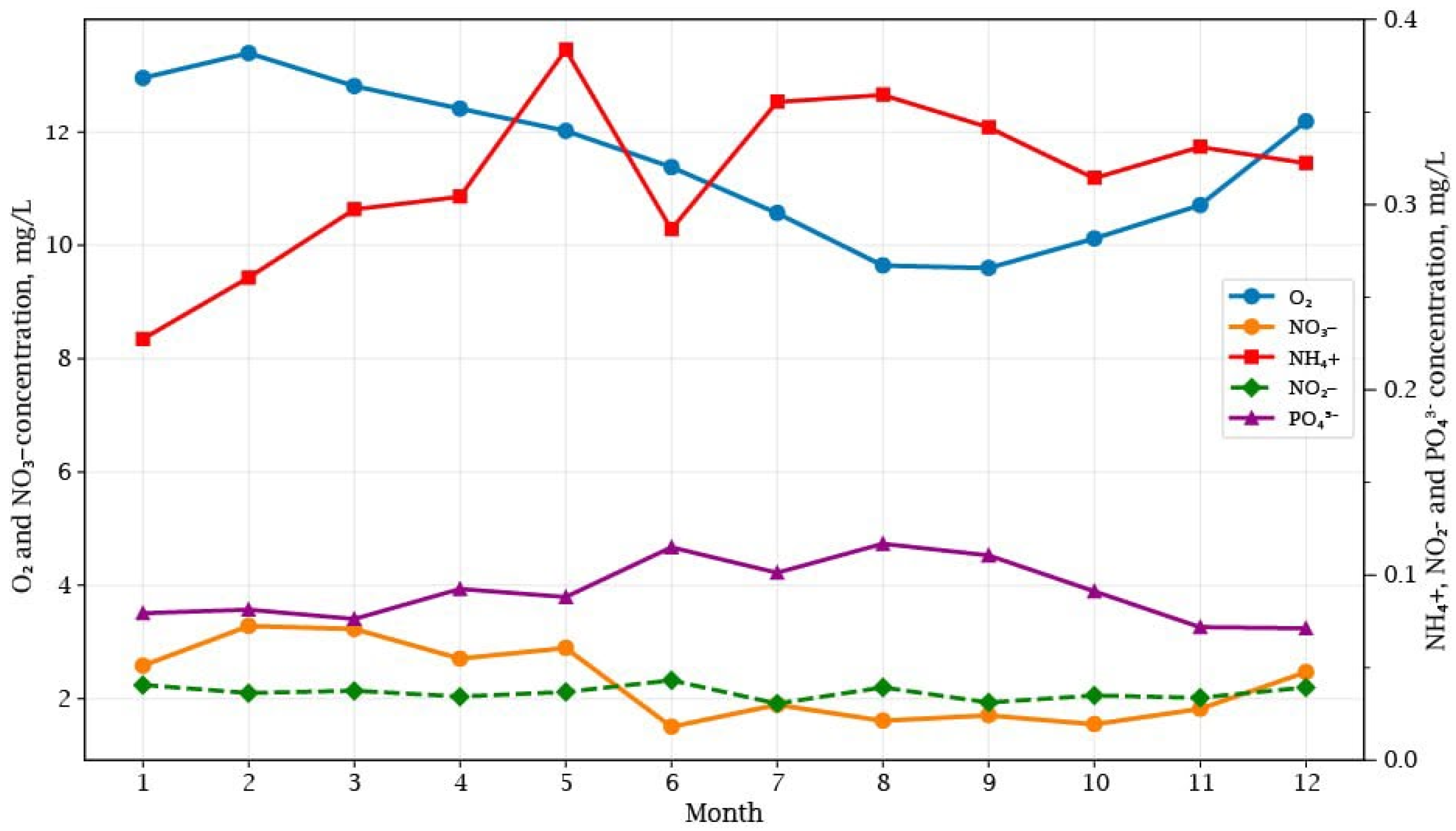
Seasonal variability of hydrochemical parameters was assessed using monthly averaged concentrations. Seasonal profiles were constructed for dissolved oxygen, ammonium, nitrites, nitrates, and phosphates. To improve visualization of variables with different concentration ranges, dual-axis plots were used, where dissolved oxygen and nitrates were displayed on the primary axis and ammonium, nitrites, and phosphates on the secondary axis.

To quantify the influence of nutrient compounds on dissolved oxygen dynamics, a Random Forest regression model was applied. Random Forest is an ensemble machine learning algorithm that combines multiple decision trees and aggregates their predictions to improve model stability and predictive performance. The method is particularly suitable for environmental datasets because it can capture nonlinear relationships and interactions among variables without requiring assumptions regarding data distribution.

In this study, dissolved oxygen concentration (O₂) was selected as the target variable, while concentrations of ammonium (NH₄⁺), nitrites (NO₂⁻), nitrates (NO₃⁻), and phosphates (PO₄³⁻) were used as predictor variables. Temporal variables (month and year) were excluded from the final model to focus exclusively on hydrochemical controls and avoid the dominance of seasonal effects.

The dataset was randomly divided into training (75%) and testing (25%) subsets. A Random Forest Regressor consisting of 500 decision trees was trained using the training dataset. Model performance was evaluated using the coefficient of determination (R²) and mean absolute error (MAE).

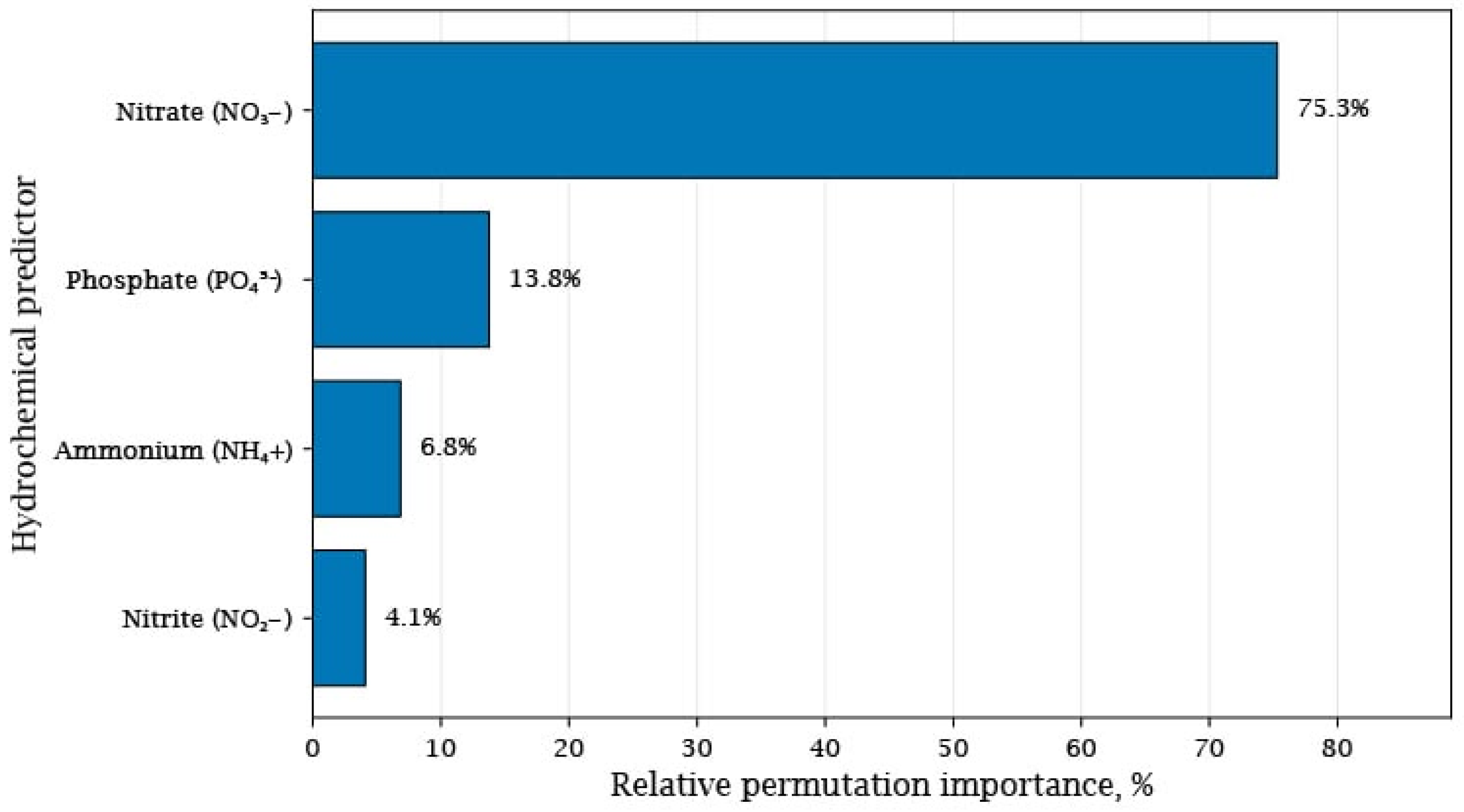
In the design of this study, we took into account the known experience [17,19] of using machine learning technologies to assess the ecological status, quality, and pollution of surface waters. To assess the contribution of individual predictors, permutation feature importance analysis was employed. This approach estimates variable importance by repeatedly shuffling the values of each predictor and measuring the resulting decrease in model performance. Variables causing the largest decline in predictive accuracy are considered the most influential factors controlling dissolved oxygen variability.

The obtained importance values were normalized and expressed as relative percentages to facilitate comparison among hydrochemical parameters. The results provide a quantitative assessment of the role of individual nutrient compounds in shaping oxygen conditions within the monitored river systems.

Cluster analysis was applied to identify groups of monitoring stations characterized by similar water quality conditions and nutrient-related ecological responses. The analysis was performed using the K-means clustering algorithm, which partitions observations into homogeneous groups by minimizing within-cluster variance and maximizing between-cluster differences.

The clustering procedure was based on mean values of water quality indices calculated for each monitoring station. The following indices were included in the analysis: dissolved Oxygen Index, Ammonium Index, Nitrite Index, Nitrate Index, Total Nitrogen Index and Phosphate Index. These indicators were selected because they represent the principal components of nutrient-related water quality assessment and provide an integrated description of ecological conditions [19].

Prior to clustering, all variables were standardized using z-score normalization to eliminate the influence of differences in measurement scales and to ensure equal contribution of each variable to the clustering process. Standardization transformed each variable to a mean value of zero and a standard deviation of one.

The K-means algorithm was implemented with 30 random initializations to improve solution stability and reduce sensitivity to initial centroid placement. Based on exploratory analysis and the limited number of monitoring stations, three clusters were selected as the optimal compromise between interpretability and differentiation of ecological conditions.

For each cluster, mean values of all water quality indices were calculated to characterize the environmental profile of the identified groups. Cluster centroids were subsequently used to interpret the dominant hydrochemical features associated with each group of monitoring stations.

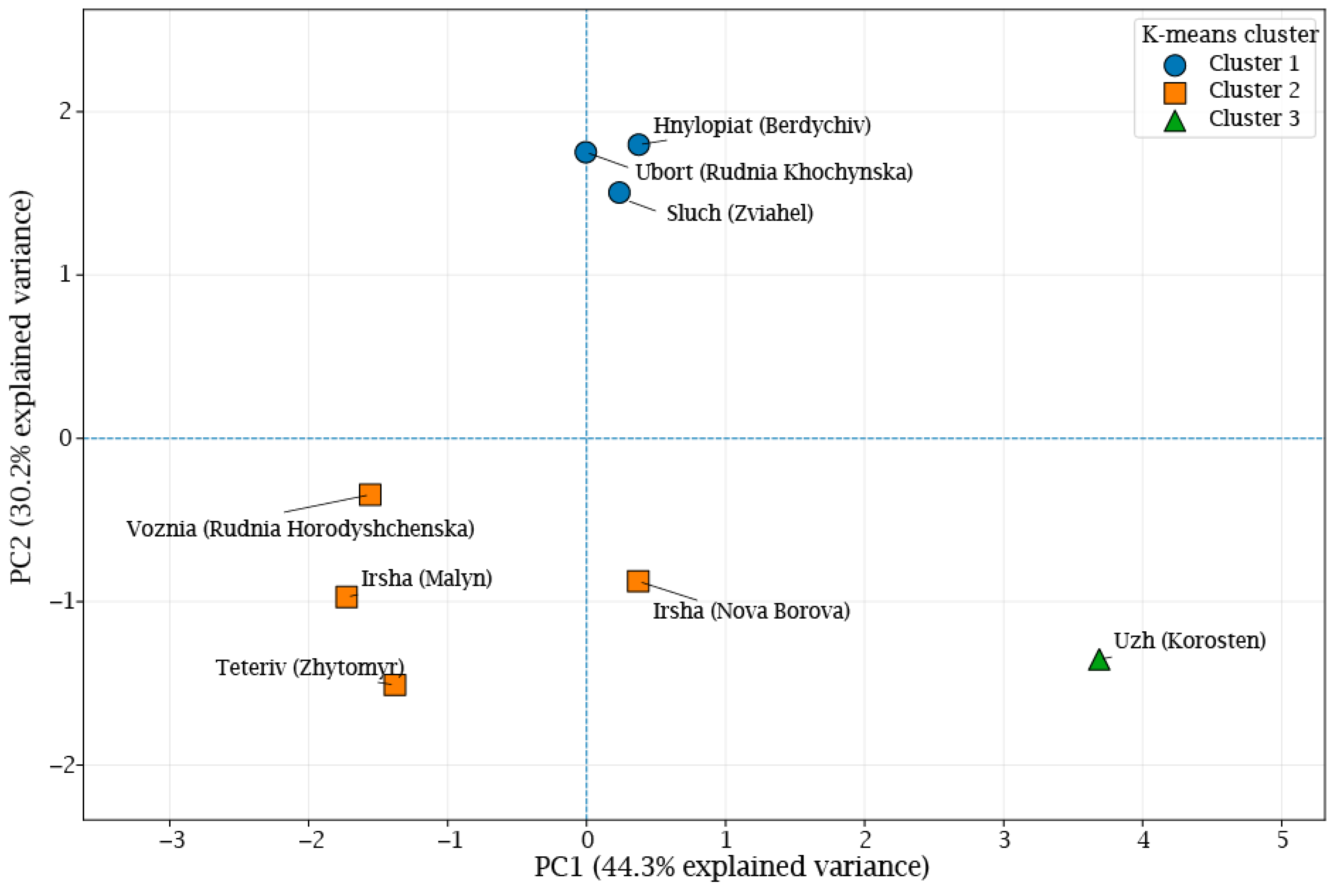
To visualize multidimensional relationships among monitoring stations and evaluate cluster separation, Principal Component Analysis (PCA) was applied. PCA transforms correlated variables into a reduced set of orthogonal components while retaining the maximum possible variance of the original dataset. The first two principal components were used for graphical representation of station similarity and cluster structure.

The resulting clusters were integrated into a GIS environment, enabling spatial visualization of cluster membership and identification of geographical patterns in water quality conditions across the Polissia region. Our choice is due to the fact that the combination of GIS and machine learning can provide valuable information [19,44] for decision-making in the final stages of intelligent surface water management.

Geospatial analysis was performed to investigate the spatial distribution of monitoring stations and the resulting cluster assignments. Geographic coordinates of monitoring sites were integrated into a GIS environment and linked with hydrochemical and clustering results.

Cluster membership obtained from the K-means algorithm was visualized using thematic mapping techniques. Monitoring stations were displayed according to their assigned cluster, enabling identification of spatial patterns in nutrient-related water quality conditions across the Polissia region. Spatial visualization facilitated interpretation of regional similarities and differences among river monitoring sites and supported the assessment of potential geographical drivers of water quality variability.

Data processing, statistical analysis, machine learning, and visualization were performed using Python (version 3.8.10). The analysis employed Pandas (version 2.0.3), NumPy (version 1.24.3), Scikit-learn (version 1.3.2), Matplotlib (version 3.7.5), GeoPandas (version 0.13.2), and OpenPyXL (version 3.1.2).

4. Case Study

4.1. Methodology

In practice, to solve the problem of assessing the status or changes in the quality of surface water resources (or their pollution level), various tools for analyzing empirical monitoring data are used, for example: correlation analysis and analysis of variance (ANOVA), factor analysis (FA), discriminant analysis (DA), principal component analysis (PCA), cluster analysis (CA) [41,45] and others. This study proposes an integrated methodology for assessing the influence of nutrient compounds on surface water quality using a combination of statistical analysis, machine learning, clustering methods, and GIS-based spatial visualization. The methodological framework was designed to identify both temporal and spatial patterns of nutrient-related water quality variability in the surface waters of the Polissia region of Ukraine.

The proposed experimental procedure was based on the known experience of solving a similar problem [15,21,22] and consisted of several consecutive stages: data preprocessing, statistical analysis of hydrochemical relationships, assessment of seasonal variability, machine learning-based evaluation of nutrient impacts on dissolved oxygen, clustering of monitoring stations according to water quality indices, dimensionality reduction using Principal Component Analysis, and GIS-based spatial visualization of the obtained results.

At the first stage, hydrochemical observations were organized into a unified analytical database. Data preprocessing included verification of records, conversion of variables into numerical format, removal of inconsistent entries, and aggregation of observations by monitoring station and sampling date. Additional temporal attributes, namely year and month, were extracted to support seasonal analysis. This stage ensured consistency of the input data and prepared the dataset for further statistical and machine learning procedures.

To evaluate linear relationships among hydrochemical parameters, the Pearson correlation coefficient was calculated [46]:

$$r_{xy}={\displaystyle \frac{{\sum }_{i=1}^n \left(x_i-\underset{¯}{x}\right)\left(y_i-\underset{¯}{y}\right)}{\sqrt{{\sum }_{i=1}^n {\left(x_i-\underset{¯}{x}\right)}^2}\sqrt{{\sum }_{i=1}^n {\left(y_i-\underset{¯}{y}\right)}^2}}},$$

(2)

where $x_i$ and $y_i$ are observed values of two hydrochemical variables, $\underset{¯}{x}$ and $\underset{¯}{y}$ are their mean values, and n is the number of observations. This metric was selected because it provides a quantitative measure of the direction and strength of linear association between nutrient compounds and dissolved oxygen. Correlation analysis was used as an exploratory tool to determine whether direct linear dependencies exist in the dataset and to justify the need for nonlinear modelling methods.

Seasonal variability was assessed by calculating monthly average concentrations of the investigated parameters:

$${\underset{¯}{X}}_m={\displaystyle \frac{1}{n_m}}{\sum }_{i=1}^{n_m} X_i,$$

(3)

where ${\underset{¯}{X}}_m$ is the mean concentration of a given hydrochemical parameter in month m, $X_i$ is an individual observation, and $n_m$ is the number of observations available for that month. Monthly aggregation was used to reduce the influence of short-term fluctuations and to reveal stable seasonal patterns associated with hydrological conditions, biological activity, nutrient transformation processes, and temperature-dependent oxygen dynamics.

Dissolved oxygen was selected as the target variable because it is one of the most informative indicators of the ecological state of river ecosystems and reflects the balance between oxygen production, consumption, reaeration, and biochemical transformation processes. The concentrations of ammonium, nitrites, nitrates, and phosphates were used as predictor variables. Temporal variables were not included in the final machine learning model in order to focus specifically on hydrochemical controls and avoid the dominance of seasonal effects.

To quantify the influence of nutrient compounds on dissolved oxygen concentration, a Random Forest regression model was applied. The general prediction of the ensemble model can be written as [47]:

$$\widehat{y}={\displaystyle \frac{1}{B}}{\sum }_{b=1}^B T_b\left(x\right),$$

(4)

where $\widehat{y}$ is the predicted dissolved oxygen concentration, $T_b\left(x\right)$ is the prediction of the b-th decision tree, B is the total number of trees, and x is the vector of predictor variables. Random Forest was selected because environmental hydrochemical data often contain nonlinear relationships, interactions among variables, and non-normally distributed observations. Unlike simple linear regression, this method does not require strict assumptions about the distribution of variables and is suitable for identifying complex patterns in environmental monitoring datasets.

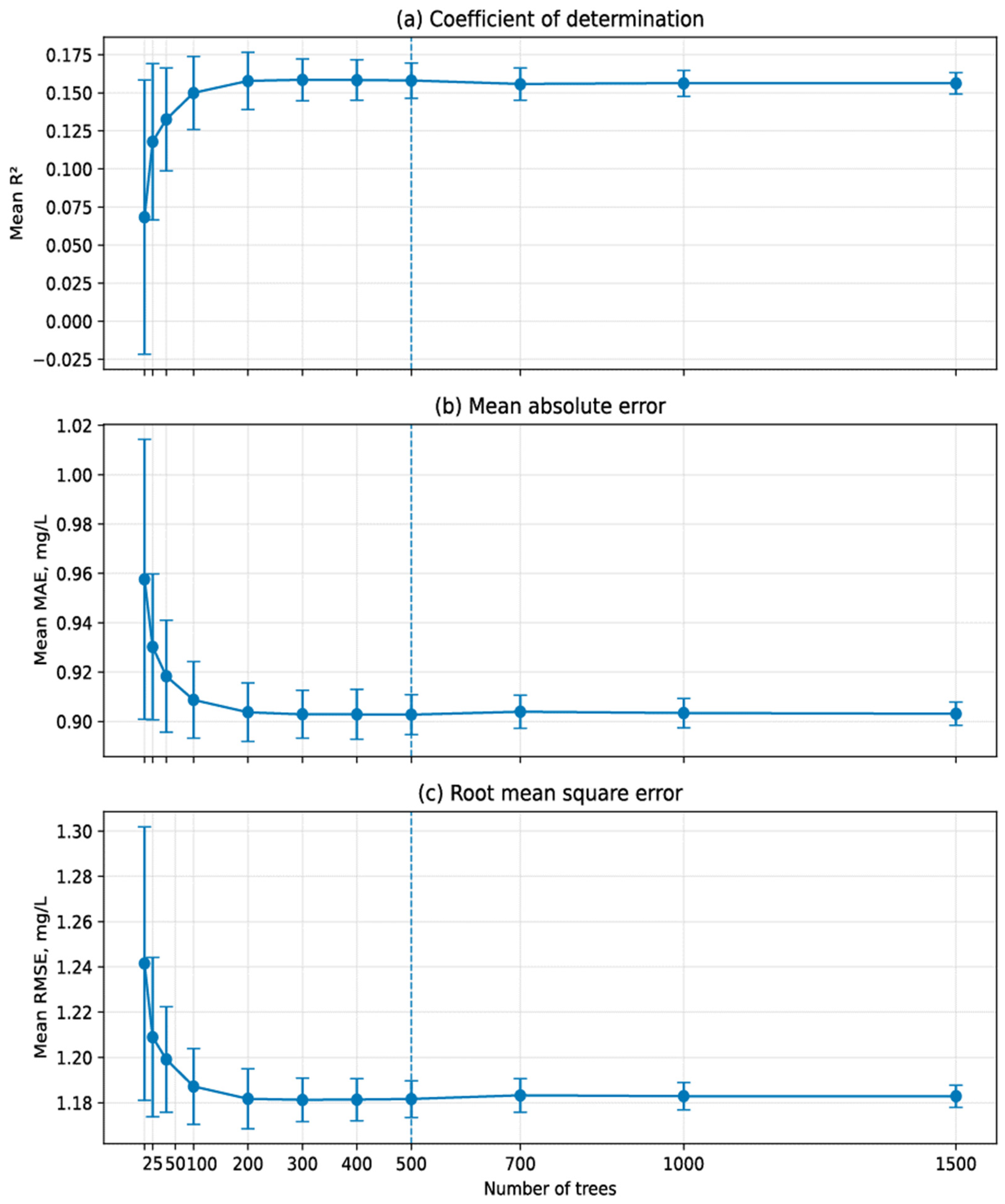
The dataset was randomly divided into training and testing subsets in the proportion of 75% and 25%, respectively. To justify the ensemble size, a sensitivity analysis was performed for 11 values of the number of trees: 10, 25, 50, 100, 200, 300, 400, 500, 700, 1000, and 1500. For each configuration, the Random Forest model was fitted 30 times using different random seeds, while the training and testing subsets remained unchanged. Model stability was assessed using the mean and standard deviation of R², MAE, and RMSE. The performance metrics improved markedly as the number of trees increased to approximately 200–300 and subsequently reached a stable plateau. At 500 trees, the model achieved a mean R² of 0.1580 ± 0.0116, a mean MAE of 0.9028 ± 0.0081 mg/L, and a mean RMSE of 1.1816 ± 0.0081 mg/L. Increasing the ensemble size beyond 500 trees changed the mean RMSE by less than 0.14% (Figure 1). Therefore, 500 trees were selected as a reasonable compromise between prediction stability and computational efficiency.

Model performance was evaluated using three complementary metrics: coefficient of determination, mean absolute error, and root mean square error. The coefficient of determination was calculated as [47]:

$$R^2=1-{\displaystyle \frac{{\sum }_{i=1}^n {\left(y_i-{\widehat{y}}_i\right)}^2}{{\sum }_{i=1}^n {\left(y_i-\underset{¯}{y}\right)}^2}},$$

(5)

where $y_i$ is the observed dissolved oxygen concentration, ${\widehat{y}}_i$ is the predicted value, and $\underset{¯}{y}$ is the mean observed value. The $R^2$ metric was used to estimate the proportion of dissolved oxygen variability explained by the selected nutrient predictors.

The mean absolute error was calculated as:

$$MAE={\displaystyle \frac{1}{n}}{\sum }_{i=1}^n \left|y_i-{\widehat{y}}_i\right|.$$

(6)

MAE was selected because it provides an easily interpretable estimate of the average prediction error in the same measurement units as dissolved oxygen concentration.

The root mean square error was calculated as:

$$RMSE=\sqrt{{\displaystyle \frac{1}{n}}{\sum }_{i=1}^n {\left(y_i-{\widehat{y}}_i\right)}^2}.$$

(7)

RMSE was included because it gives greater weight to larger prediction errors and therefore allows assessment of the model’s sensitivity to substantial deviations between observed and predicted values. The combined use of $R^2$, MAE, and RMSE provides a more complete evaluation of model performance than any single metric alone.

To assess the relative contribution of individual nutrient compounds to dissolved oxygen variability, permutation feature importance was applied. The importance of the j-th predictor was defined as [47]:

$${PI}_j={Perf}_{base}-{Perf}_{perm,j},$$

(8)

where ${Perf}_{base}$ is the baseline model performance and ${Perf}_{perm,j}$ is the model performance after random permutation of the values of predictor j. A larger decrease in performance indicates a greater importance of the corresponding variable. The obtained importance values were normalized and expressed as relative percentages to facilitate comparison among hydrochemical parameters.

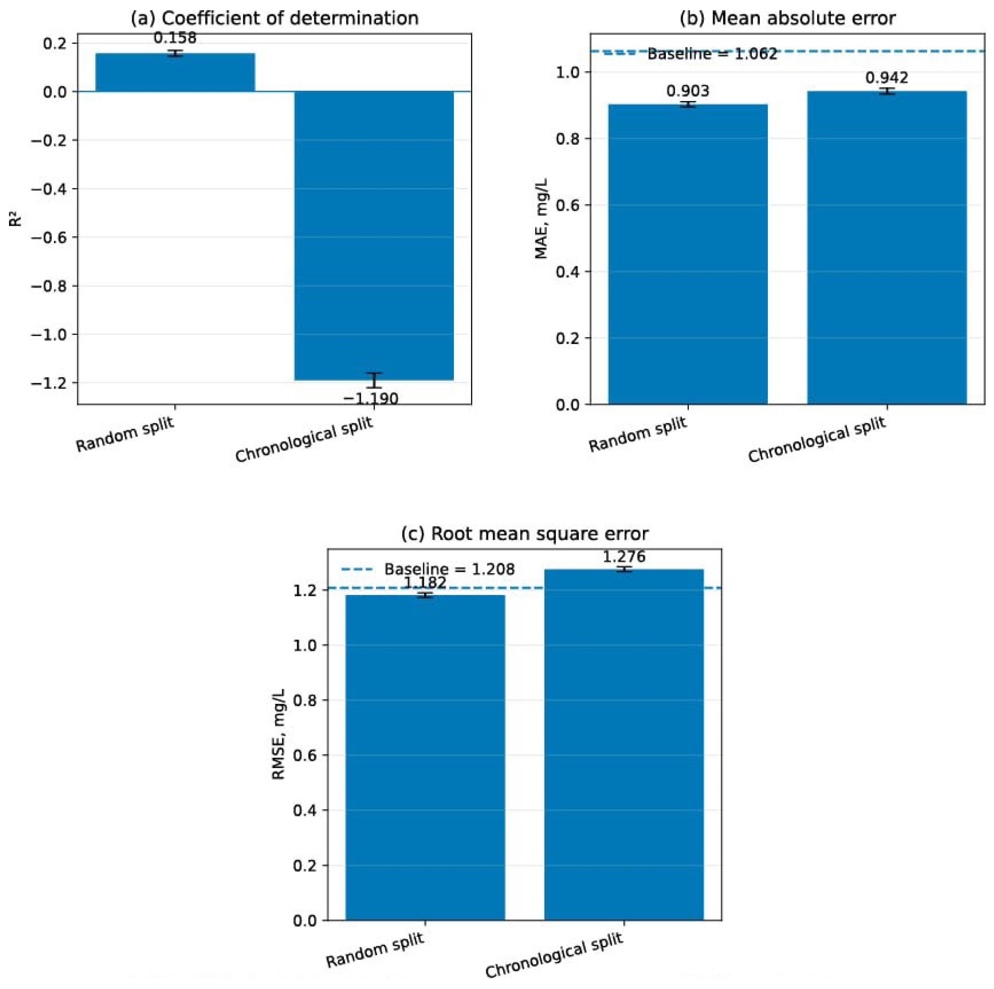
To assess the influence of the validation strategy on model performance, an additional chronological validation was conducted. In this approach, the first 75% of the monitoring period (January 2024–June 2025) was used for model training, whereas the remaining 25% (June 2025–December 2025) served as an independent testing dataset. Unlike random sampling, this procedure preserves the temporal order of observations and minimizes the potential influence of temporal autocorrelation on model evaluation. The predictive performance obtained using the chronological split was subsequently compared with that of the conventional random train–test split to evaluate the robustness of the Random Forest model under a more conservative validation framework (Figure 2).

The relatively small standard deviations obtained across the 30 repeated model fits indicate that the observed differences between the random and chronological validation strategies are stable and reproducible rather than being caused by random initialization of the ensemble.

At the next stage, cluster analysis was used to identify groups of monitoring stations with similar nutrient-related water quality conditions. The K-means algorithm was applied to mean values of water quality indices calculated for each monitoring station. The following indices were included in the clustering procedure: dissolved Oxygen Index, Ammonium Index, Nitrite Index, Nitrate Index, Total Nitrogen Index, and Phosphate Index. These indicators were selected because they represent the main components of nutrient-related water quality assessment and provide an integrated description of ecological conditions.

The K-means algorithm minimizes the within-cluster sum of squared distances [48]:

$$J={\sum }_{k=1}^K {\sum }_{x_i\in C_k} {\Vert x_i-{\mu }_k\Vert }^2,$$

(9)

where K is the number of clusters, $C_k$ is the set of observations assigned to cluster k, $x_i$ is an observation vector, and ${\mu }_k$ is the centroid of the corresponding cluster. The method partitions monitoring stations into homogeneous groups by minimizing within-cluster variability and maximizing differences between clusters.

Prior to clustering, all variables were standardized using z-score normalization [44]:

$$z_i={\displaystyle \frac{x_i-\mu }{\sigma }},$$

(10)

where $x_i$ is the original value, $\mu$ is the mean value of the variable, and $\sigma$ is its standard deviation. Standardization was necessary because the water quality indices have different numerical ranges, and without normalization variables with larger absolute values could dominate the clustering procedure.

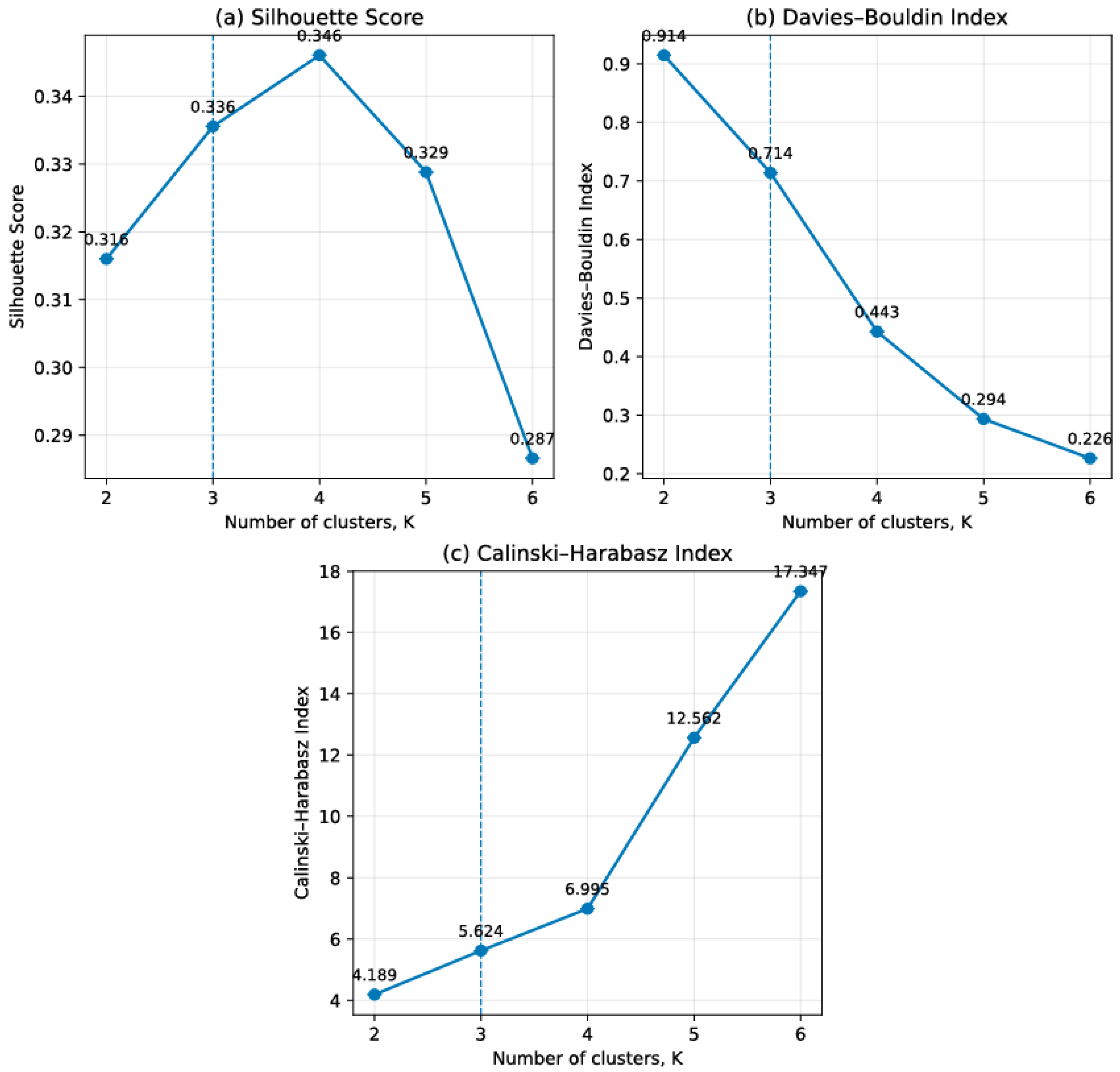
The K-means algorithm was implemented with 30 random initializations to improve the stability of the final clustering solution and reduce sensitivity to initial centroid placement. To justify the selection of the number of clusters, additional structural validation was performed by comparing solutions with K = 2 and K = 3 using the Silhouette Score, Davies–Bouldin Index, and Calinski–Harabasz Index. The three-cluster solution consistently demonstrated better internal validation metrics (Silhouette Score = 0.336 vs. 0.316; Davies–Bouldin Index = 0.714 vs. 0.915; Calinski–Harabasz Index = 5.624 vs. 4.189), while both solutions exhibited identical clustering stability (Adjusted Rand Index = 1.0). Although higher values of K further improved some internal validation indices, these solutions fragmented the dataset of eight monitoring stations into very small clusters containing only one or two stations, thereby reducing their ecological interpretability. Therefore, the three-cluster solution was selected as the best compromise between statistical quality and environmental interpretability (Figure 3).

To visualize multidimensional relationships among monitoring stations and assess cluster separation, Principal Component Analysis was applied. PCA transforms the original standardized variables into a new set of uncorrelated components [49]:

$$Z=XW,$$

(11)

where X is the standardized data matrix, W is the matrix of eigenvectors, and Z is the matrix of principal component scores. The first two principal components were used for graphical representation because they retain the largest share of total variance and allow interpretation of similarities and differences among monitoring stations in a reduced two-dimensional space.

At the final stage, the results of cluster analysis were integrated into a GIS environment. Combining machine learning technologies with traditional analysis methods [24,50] provides better classification and clustering results in conditions of uncertainty and lack of empirical data for analysis. Geographic coordinates of the monitoring stations were linked with hydrochemical characteristics and cluster assignments. GIS-based visualization made it possible to display the spatial distribution of nutrient-related water quality types, identify regional heterogeneity, and determine whether the observed differences were associated with geographical location or local catchment-specific factors.

All stages of data processing, statistical analysis, machine learning, clustering, dimensionality reduction, and visualization were implemented Python (version 3.8.10). Pandas (version 2.0.3) and NumPy (version 1.24.3) were used for data preprocessing and numerical calculations; Scikit-learn (version 1.3.2) was used for Random Forest regression, permutation importance, K-means clustering, and PCA; Matplotlib (version 3.7.5) was used for graphical visualization; GeoPandas (version 0.13.2) was used for spatial data processing and thematic mapping; and OpenPyXL (version 3.1.2) was used for working with tabular data files.

Thus, the proposed methodology provides a consistent analytical framework for assessing nutrient impacts on surface water quality. The combination of correlation analysis, seasonal aggregation, Random Forest modelling, permutation importance, cluster analysis, PCA, and GIS visualization enables both quantitative evaluation of hydrochemical relationships and spatial interpretation of ecological differences among river monitoring stations.

4.2. Results

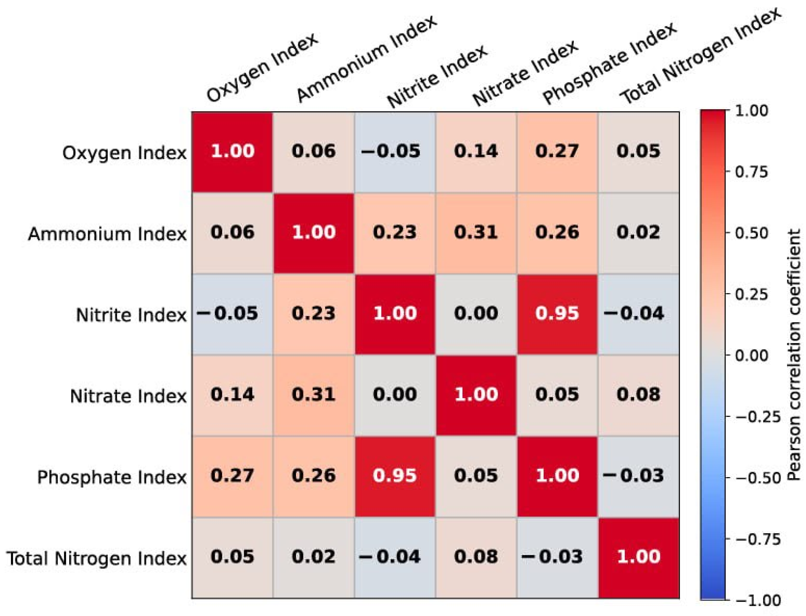
Correlation analysis revealed generally weak relationships among the investigated hydrochemical parameters (Figure 4). The strongest positive correlation was observed between dissolved oxygen and nitrate concentration (r = 0.35), indicating that higher nitrate concentrations tend to be associated with slightly elevated oxygen levels. However, the magnitude of this relationship suggests only a weak-to-moderate association.

A moderate positive relationship was also identified between phosphate and nitrite concentrations (r = 0.31), which may indicate common nutrient sources or similar biogeochemical transformation pathways. Nitrite concentration showed a weaker positive correlation with nitrates (r = 0.23), suggesting partial coupling of nitrogen transformation processes within the aquatic environment.

Negative correlations were observed between dissolved oxygen and ammonium (r = −0.26) as well as dissolved oxygen and phosphates (r = −0.28). These relationships are consistent with the tendency of increased nutrient loading to be associated with oxygen consumption during decomposition and biochemical transformation processes. Nevertheless, the relatively low correlation coefficients indicate that nutrient concentrations alone do not fully explain oxygen dynamics in the studied river systems.

Virtually no relationship was detected between nitrates and phosphates (r = 0.00), suggesting independent variability of these nutrient groups within the monitoring dataset. This indicates different mechanisms and sources of these nutrients entering the water sub-mass: if nitrates mainly come from diffuse and non-point source pollution sources (e.g., agricultural lands), then phosphate water pollution mainly occurs from point sources and “hot spots” (e.g., Human Wastewater and Urban Runoff with phosphate residues from detergents). Similarly, ammonium exhibited only negligible correlations with nitrites (r = 0.06) and nitrates (r = −0.05).

Overall, the correlation structure indicates that the hydrochemical regime of the monitored rivers is controlled by multiple interacting environmental factors rather than by direct linear relationships among individual nutrient compounds. The predominance of weak correlations also supports the application of machine learning methods capable of identifying nonlinear relationships within the dataset.

The seasonal profiles of dissolved oxygen and nutrient compounds demonstrate pronounced temporal variability throughout the year (Figure 5). The presented curves were constructed using mean monthly concentrations calculated from all observations collected during the 2024–2025 monitoring period. The observed patterns indicate the influence of seasonal hydrological conditions, biological activity, and nutrient transformation processes within the river ecosystems of the Polissia region during different vegetation seasons.

Dissolved oxygen concentrations exhibited a clear annual cycle. The highest values were observed during winter and early spring (January–March), reaching approximately 13.0–13.4 mg/L. Oxygen concentrations gradually declined during late spring and summer, reaching a minimum of approximately 9.6 mg/L in August–September. Subsequently, oxygen levels increased again during autumn and early winter. This pattern is primarily associated with seasonal water temperature variations, as oxygen solubility decreases with increasing temperature, while biological oxygen consumption intensifies during the warm period.

Nitrate concentrations (NO₃⁻) displayed moderate seasonal variability. Maximum concentrations were observed during late winter and spring (February–May), reaching approximately 2.8–3.3 mg/L. A pronounced decrease occurred in June, when concentrations dropped to about 1.5 mg/L. Lower nitrate concentrations persisted throughout summer and autumn before increasing again in December. This seasonal behaviour is consistent with enhanced nutrient uptake by aquatic vegetation during the growing season and reduced biological assimilation during colder months.

Among the investigated nutrient compounds, ammonium (NH₄⁺) exhibited the highest seasonal variability. Concentrations increased steadily from winter to late spring, reaching a maximum of approximately 0.39 mg/L in May. Following a temporary decline in June, elevated ammonium concentrations persisted during summer and early autumn. Such fluctuations may reflect seasonal changes in organic matter decomposition, microbial activity, and local nutrient inputs from the catchment area.

Nitrite concentrations (NO₂⁻) remained relatively stable throughout the year, varying within a narrow range of approximately 0.035–0.050 mg/L. The absence of pronounced seasonal peaks suggests that nitrites represent a transitional component of the nitrogen cycle and are rapidly transformed into other nitrogen forms under prevailing environmental conditions.

Phosphate concentrations (PO₄³⁻) demonstrated a seasonal pattern characterized by elevated values during summer and early autumn. The highest concentrations, exceeding 0.11 mg/L, were observed during June–September, whereas lower values occurred during winter months. This behaviour may indicate enhanced phosphorus release from bottom sediments, intensified mineralization processes, and increased anthropogenic inputs during the warm period.

Overall, the seasonal analysis indicates that dissolved oxygen follows a pattern opposite to that of nutrient enrichment, particularly during summer months. The simultaneous reduction in oxygen concentrations and increase in ammonium and phosphate levels during the warm season suggests intensified biological and biogeochemical processes. These results confirm the importance of seasonal factors in controlling nutrient dynamics and ecological conditions in the monitored river systems.

To evaluate the relative contribution of nutrient compounds to dissolved oxygen variability, a Random Forest regression model was applied. Dissolved oxygen concentration was used as the target variable, while ammonium, nitrite, nitrate, and phosphate concentrations served as predictors. The analysis was conducted without temporal variables to focus specifically on hydrochemical influences. Because preliminary correlation analysis indicated weak linear relationships among hydrochemical variables, a machine learning approach was employed to identify potentially nonlinear patterns affecting dissolved oxygen variability.

Model performance metrics indicated limited predictive capability (R² = 0.154, MAE = 0.922 mg/L, RMSE = 1.184 mg/L). These values suggest that nutrient concentrations alone explain only a relatively small proportion of dissolved oxygen variability. This result should be interpreted as evidence of the limited explanatory power of the selected nutrient predictors rather than as evidence for the absence of industrial, accidental, or other anthropogenic pollution. Since the model included only nutrient-related variables, it did not account for other potential pollutants or important environmental drivers, such as water temperature, hydrological conditions, organic matter decomposition, biological productivity, and atmospheric reaeration, which may also substantially influence dissolved oxygen dynamics within the studied river systems.

An additional chronological validation (Figure 2) produced more conservative performance estimates than the conventional random split. The mean coefficient of determination decreased from 0.158 ± 0.012 to −1.190 ± 0.030, while the mean MAE increased from 0.903 ± 0.008 to 0.942 ± 0.009 mg/L and the mean RMSE increased from 1.182 ± 0.008 to 1.276 ± 0.009 mg/L. These findings indicate that the predictive performance of the Random Forest model is sensitive to the validation strategy and further confirm that nutrient variables alone are insufficient for reliable temporal prediction of dissolved oxygen. The observed deterioration in performance under chronological validation highlights the need to incorporate additional hydro-meteorological predictors, including water temperature, river discharge, flow velocity, and seasonal characteristics, in future model development.

Despite the modest predictive performance, the Random Forest model provided valuable information regarding the relative importance of individual hydrochemical variables (Figure 6). Permutation importance analysis revealed that nitrate concentration (NO₃⁻) was by far the most influential predictor, accounting for approximately 75% of the total relative importance.

Phosphate concentration (PO₄³⁻) represented the second most important variable with a contribution of approximately 14%, while ammonium concentration (NH₄⁺) accounted for about 7%. Nitrite concentration (NO₂⁻) exhibited the lowest contribution, representing approximately 4% of total model importance.

The pronounced dominance of nitrate importance suggests that nitrate dynamics are more strongly associated with dissolved oxygen variability than other investigated nutrient forms. This finding may reflect the influence of nitrogen transport from the catchment, nutrient cycling processes, and biological transformations occurring within river ecosystems.

Although the model was not intended as a predictive tool, the feature importance ranking provides insight into the relative contribution of nutrient compounds to oxygen dynamics. Among the investigated hydrochemical parameters, nitrates can therefore be considered the most informative indicator associated with dissolved oxygen variability in the monitored rivers of the Polissia region. The dominance of nitrates indirectly indicates that nitrification processes (nitrogen cycle in the aquatic ecosystem) shape the oxygen regime of the basin waters in the study region.

To identify groups of monitoring stations with similar hydrochemical characteristics, K-means clustering was applied using water quality indices as input variables. The analysis resulted in three distinct clusters representing different ecological conditions and nutrient-related water quality patterns.

The separation of monitoring stations in the multidimensional space is illustrated by Principal Component Analysis (PCA) (Figure 7). The first two principal components explained 74.5% of the total variance (PC1 = 44.3%, PC2 = 30.2%), indicating that the PCA representation adequately captures the dominant structure of the dataset.

The PCA diagram demonstrates a clear differentiation among the identified clusters, indicating that the selected water quality indices effectively characterize distinct hydrochemical conditions. Monitoring stations grouped within the same cluster exhibit similar ecological profiles, whereas stations belonging to different clusters are characterized by contrasting nutrient and water quality conditions.

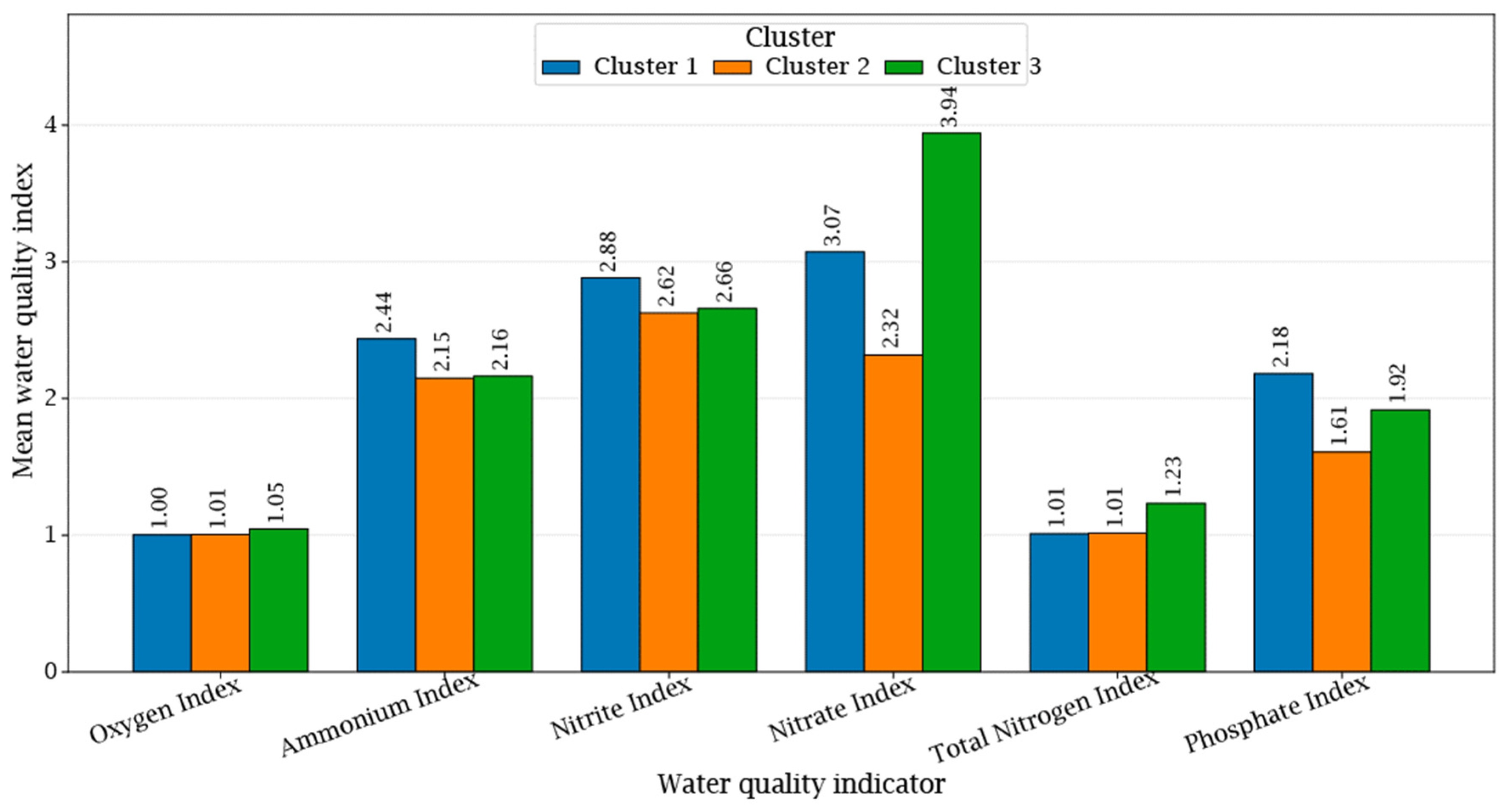
The ecological characteristics of the identified clusters are presented in Figure 8. Mean values of water quality indices reveal distinct hydrochemical profiles among the three groups of monitoring stations.

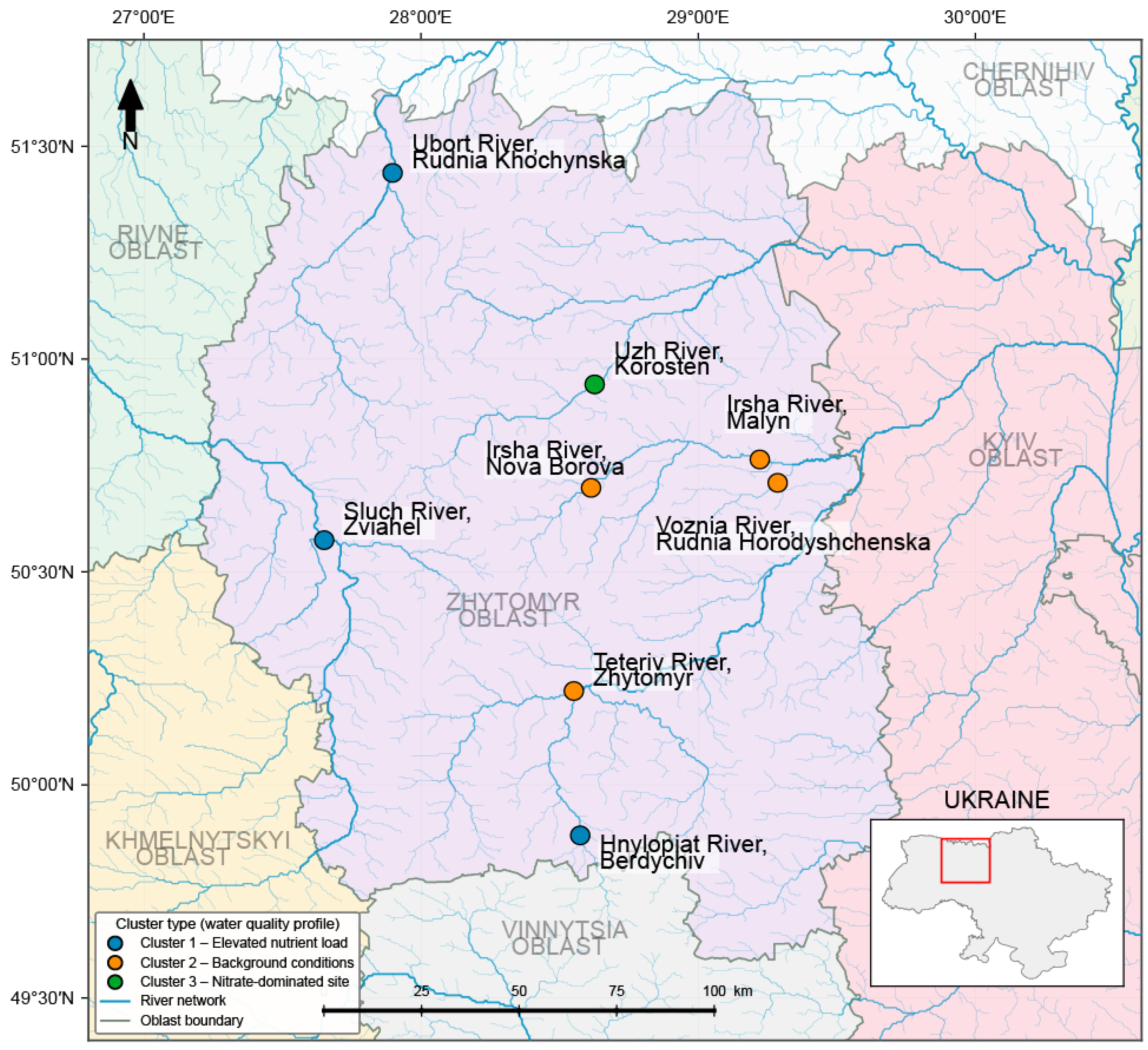
Cluster 1 includes the monitoring stations located at the Hnylopiat, Sluch, and Ubort rivers. This cluster is characterized by elevated values of the Ammonium Index (Ammonium Index ≈ 2.4), Nitrite Index (Nitrite Index ≈ 2.9), Phosphate Index (Phosphate Index ≈ 2.2), and relatively high Nitrate Index values (Nitrate Index ≈ 3.1). The simultaneous increase in several nutrient-related indices indicates enhanced nutrient pressure and a more pronounced anthropogenic influence compared to other monitoring sites.

Cluster 2 comprises monitoring stations located on the Teteriv, Irsha, and Voznia rivers, including both monitoring sites situated on the Irsha River. This group exhibits the lowest values for most nutrient-related indices, particularly nitrate (Nitrate Index ≈ 2.3) and phosphate (Phosphate Index ≈1.6). These characteristics suggest comparatively favourable water quality conditions and lower nutrient enrichment. Consequently, Cluster 2 may be interpreted as representing relatively background or less impacted environmental conditions within the study area.

Cluster 3 contained a single monitoring station located on the Uzh River near Korosten. Although represented by a single monitoring site, this cluster was retained because the three-cluster solution demonstrated better structural validation than the two-cluster solution (Silhouette Score = 0.336 vs. 0.316; Davies–Bouldin Index = 0.714 vs. 0.915; Calinski–Harabasz Index = 5.624 vs. 4.189), while maintaining identical clustering stability (Adjusted Rand Index = 1.0). Furthermore, the isolated position of this monitoring station was consistently confirmed by the Principal Component Analysis (Figure 3), indicating that it represents a hydrochemically distinct outlier rather than an artefact of the clustering algorithm. This cluster is distinguished by the highest Nitrate Index value (Nitrate Index ≈ 3.9), which substantially exceeds the values observed in the other clusters. Elevated values of the Total Nitrogen Index (Total Nitrogen Index≈ 1.2) further support the predominance of nitrogen-related impacts at this site, whereas ammonium and nitrite indices remain comparatively moderate. Consequently, Cluster 3 can be interpreted as a nitrate-dominated hydrochemical outlier within the study area.

The cluster structure demonstrates that nutrient-related water quality conditions are heterogeneous across the monitored river systems. While most monitoring stations can be grouped into clusters representing either elevated nutrient pressure or comparatively background conditions, the Uzh River monitoring site forms a distinct hydrochemical category associated primarily with nitrate enrichment.

The spatial distribution of monitoring station clusters in the Polissia region is presented in Figure 9. Integration of clustering results into the GIS environment enabled visualization of geographical patterns in nutrient-related water quality conditions across the study area.

The spatial arrangement of clusters does not indicate a simple geographical gradient. Instead, stations located within relatively close proximity may belong to different clusters, reflecting the influence of local catchment characteristics, land-use patterns, hydrological connectivity, and anthropogenic pressures on nutrient dynamics and water quality conditions.

The occurrence of nutrient-enriched, background-condition, and nitrate-dominated clusters across different parts of the study area suggests that local environmental controls play a greater role than geographical location alone in determining water quality characteristics.

The integration of cluster analysis with GIS-based visualization proved effective for identifying spatial patterns in nutrient-related water quality variability. The results highlight priority areas for environmental monitoring and support the development of targeted management measures aimed at reducing nutrient inputs and improving ecological conditions within river systems of the Polissia region.

5. Discussion

5.1. Study Results Interpretation

We selected dissolved oxygen as the primary predictive variable for machine learning and analysis in this case study. We attribute this choice to the fact that the dissolved oxygen (DO) monitoring parameter is the most representative integral indicator of the tropho-saprobiological state of a water sub-body [30]. Furthermore, analyzing dissolved oxygen content in conjunction with changes in other hydrochemical parameters allows for evaluating the activity of self-purification processes and the overall resilience of the aquatic ecosystem [29].

Applying a Random Forest Regressor to quantify the impact of dissolved concentrations of ammonium, nitrites, nitrates, and phosphates on dissolved oxygen levels demonstrated a specific, statistically limited predictive capacity. The baseline model metrics recorded a coefficient of determination (R²) of only 0.154 (MAE = 0.922 mg/L, RMSE = 1.184 mg/L). In traditional hydrochemical modelling tasks, such a value is insufficient. For instance, analogous studies utilizing a hybrid deep learning architecture (CNN-LSTM) to predict nitrate content based on routine monitoring parameters demonstrate a Nash–Sutcliffe efficiency (NSE) score exceeding 0.70 [13].

In the context of this case study, the low coefficient of determination holds analytical value, as it indicates a marginal impact of biogenic element concentrations on the variability of dissolved oxygen in the waters of the studied Pripyat River and Middle Dnieper River sub-basins. Drawing an analogy to the results of study [12], this fact indirectly supports the hypothesis that there has been no dominant influence from industrial or “hot-spot” pollution in the studied sub-basins of the Ukrainian Polissya over a medium-term retrospective period. The statistically limited predictive capacity of the model suggests that dissolved oxygen dynamics in the aquatic ecosystems of the Ukrainian Polissya river sub-basins depend on non-anthropogenic and physicochemical factors. These include hydrological regime (flow velocity and turbulence) or thermal regime (water temperature inversely regulates the physical solubility of gases); different biochemical processes (the rate of microbial decomposition of autochthonous and allochthonous organic matter) or factors (the intensity of primary biological productivity of macrophytes and phytoplankton, among others).

Despite the limitations of the case study, the chosen methodological approach and the permutation feature importance analysis successfully identified the hierarchy of nutrient impacts on the oxygen balance inherent to this water sub-body. The clear and unambiguous distribution of predictor importance confirms that the hydrochemical water quality of the sub-basin is shaped by the dominant influence of nitrification processes and the diffuse input of nitrate nitrogen.

Detailing the seasonal changes in the concentration of biogenic elements in the sub-basin waters (

Table 3. Seasonal profiles of changes in key hydrochemical parameters of the Ukrainian Polissya region rivers.

Hydrochemical Parameter	Dynamics and Extremes		Explanations and Comments
	Winter–Spring Period	Summer–Autumn Active Vegetation Period
Dissolved oxygen (DO)	Maximum: 13.0–13.4 mg/L (January–March, the period before spring flooding start)	Minimum: ~9.6 mg/L (August–September)	The cycle of parameter changes can be explained by the influence of the average daily temperature (Henry’s law, the solubility of gases decreases with increasing temperature) and the balance between oxygen photosynthesis and BOD for the decomposition of organic matter in the summer.
Nitrates (NO3−)	Maximum: 2.8–3.3 mg/L (February–May, waterlogging period)	Decrease to ~1.5 mg/L (June–September, active vegetation period)	The increase in nitrate pollution in spring is associated with the combined effect of factors: the activity of surface and diffuse pollution in the catchment area and the absence of active biological assimilation of nitrogen in the aquatic ecosystem. The decrease in water nitrates pollution in the summer months is the result of active biological assimilation by aquatic vegetation.
Ammonium (NH4+)	Gradual increase to maximum in May: ~0.39 mg/L	Steadily increased concentration in July–September: 0.35–0.36 mg/L	Such fluctuations may reflect seasonal changes in organic matter decomposition, microbial activity, and local nutrient inputs from the catchment area.
Phosphates (PO43−)	Constantly low values in winter months	Maximum during active vegetation period (June–September): >0.11 mg/L	This behaviour may indicate enhanced phosphorus release from bottom sediments, intensified mineralization processes, and increased anthropogenic inputs during the warm period.
Nitrites (NO2−)	Stable values in a narrow range of 0.035–0.050 mg/L		The absence of pronounced seasonal peaks suggests that nitrites represent a transitional component of the nitrogen cycle and are rapidly transformed into other nitrogen forms under prevailing environmental conditions.

) is an undeniable strength of this study. These findings supplement the results of similar research on the hydroecological and hydrochemical properties of Ukrainian Polissya rivers [15,29,31]. Understanding background seasonal profiles establishes a reliable, empirically validated foundation for the future implementation of machine learning algorithms aimed at detecting anomalous deviations.

The methodological approach adopted in this study has demonstrated its effectiveness in addressing complex environmental challenges under crisis conditions characterized by limited data access and resource scarcity. The integration of correlation analysis, machine learning, and geospatial clustering enabled the identification of correlation dependencies and seasonal profiles of biogenic element (nutrient) variations within the sub-basin waters. Furthermore, it established an evidence-based foundation for water resource management at the local and sub-regional levels, using the river sub-basins of the Ukrainian Polissya as a case study (

Table 4. Main assessment results of biogenic elements’ impacts on surface water quality using machine learning analysis.

Water Monitoring Parameter	Identified Changes and Relationships	Results Supporting the Result	Hydrochemical and Ecological Changes Hypotheses	Water Resources Management and Pollution Prevention Opportunities
Total nitrate nitrogen (N-NO3−)	Most influential predictor of DO variability. Key indicator of ecological quality.	RF relative importance: ~75%. DO correlation: r = 0.35. Max: 2.8–3.3 mg/L (Feb–May). Cluster 3 (Uzh River): Nitrate-dominant.	Nitrification shapes DO regime. Summer decrease due to bio-assimilation.	Use as primary predictor in ML for risk assessment.
Total phosphorus phosphate (P-PO43+)	Second most influential variable for DO. Pronounced summer concentration increase.	RF relative importance: ~14%. DO correlation: r = −0.28. Max: >0.11 mg/L (June–Sept).	Summer increase linked to organic mineralization and point sources.	Apply ML anomaly detection for early response to point pollution.
Total ammonia nitrogen (TAN, N-NH4+)	Highest seasonal variability. Indirectly worsens water quality (Cluster 1)	RF relative importance: ~7%. DO correlation: r = −0.26. Max peak in May: ~0.39 mg/L.	Changes are related to secondary factors (microbial activity, organic decomposition).	Use as secondary predictor in complex analytical cases. Helps prioritize nature-based solutions.
Total nitrite nitrogen (N-NO2−)	Smallest contribution to DO variability. Stable concentrations throughout the year	RF relative importance: ~4%. Range: 0.035–0.050 mg/L. Positive correlation with P-PO4 (r = 0.31).	Transient component of the nitrogen cycle. Rapidly transformed into other forms.	Use as a basic indicator for ML tuning. Track emergencies in nitrogen cycle balance.

).

5.2. Limitations, Assumptions, and Methodological Trade-Offs

Modelling complex, open, and dynamic natural ecosystems requires methodological trade-offs. The authors of this case study acknowledge making deliberate assumptions, which simultaneously establish the objective boundaries of the model’s applicability and ensure the possibility of deriving robust and evidence-based management conclusions under conditions of scarce representative empirical data. Overall, the limitations in this case study can be classified into three primary areas:

(A)

Deliberate exclusion of temporal and hydrophysical variables from the machine learning model. The most prominent and debatable methodological trade-off was the authors’ decision to exclude temporal attributes (e.g., month ordinal number, season, or year), as well as key temperature and hydrological parameters, from the overall set of predictors in the Random Forest Regression model. In isolation from other factors, this decision enabled the investigation of weak correlations between the hydrochemical parameters of water quality and the ecological safety of aquatic ecosystems.

(B)

Use of calculated indices instead of absolute metric concentrations for clustering purposes. To perform multi-criteria spatial clustering using the K-means algorithm, the authors opted to use derived calculated water quality indices (Oxygen Index, Ammonium Index, Nitrite Index, Nitrate Index, Total Nitrogen Index, Phosphate Index). However, this methodological trade-off is justified given the applied managerial focus of the study. In the context of this case study, the use of indices serves as a powerful standardization tool, transforming metric results into relative dimensionless values (ranging from 1 to 7). This allows for the accurate comparison of parameters that vary by several orders of magnitude in the natural environment. Additionally, the water quality index establishes a reliable link between laboratory measurement results and the formal assessment of the ecological status and safety of water resources according to the criteria of the EU Water Framework Directive.

(C)

Limitations in the spatial and temporal representativeness of the sample. The third significant limitation is related to the volume and spatial coverage of the available empirical data. The study relies on a medium-term retrospective observation period (January 2024–December 2025) and a restricted spatial network consisting of eight official state monitoring stations located within the Pripyat River and Middle Dnieper sub-basins. Although the hydrochemical dataset comprised repeated monthly observations, the spatial clustering analysis was performed at the monitoring station level. Consequently, the limited number of monitoring stations may reduce the robustness of the identified clusters and limit the generalizability of both the clustering and machine learning results beyond the investigated monitoring network. Therefore, the obtained spatial patterns should be interpreted as representative of the analyzed monitoring stations rather than universally applicable to all river systems of the Ukrainian Polissia. Future research should expand the monitoring network, include additional observation sites, and extend the monitoring period to improve the robustness, spatial representativeness, and generalizability of the proposed analytical framework.

5.3. Opportunities for Further Research

This case study opens several promising avenues for scientific research and the practical development of a comprehensive ecosystem for the intelligent management of sub-basin water resources. To achieve this strategic goal, we plan to further develop this research along three primary directions:

• Expanding the Feature Space of Hybrid Models to Increase Predictive Accuracy: Despite the informative value of nitrate content as the primary hydrochemical predictor of the dissolved oxygen regime, subsequent modelling iterations must deliberately expand the set of input variables. Drawing on global experience [11,13] with multimodal datasets, it would be appropriate to augment the baseline predictor matrix of the Random Forest model with additional data blocks encompassing hydrological parameters, meteorological data, and landscape metrics.
• Integration of Advanced Time-Series Forecasting Methods: The seasonal profiles of variations in biogenic element and dissolved oxygen concentrations identified during the case study provide an empirical and mathematical foundation for a strategic transition toward predictive modelling of future water body states. In subsequent modelling iterations, it is necessary to expand the retrospective ranges of empirical data and increase the number of water monitoring sites. This will facilitate the integration of the Prophet additive model [11,21], enabling reliable forecasting of key hydrochemical indicator dynamics, even under conditions of a deficit in operational empirical water monitoring data.
• Development of an Integrated Decision-Support Framework for Managing Water Quality and Pollution. The combination of machine learning methods and geospatial clustering of ecological water monitoring data demonstrates analytical efficiency and prospects for use in the water resources management system at the sub-regional level. Analysis of the case study results allowed us to form a list of three promising vectors of practical water resources and environmental safety management:
  • The first practical management vector—management under uncertainty and resource scarcity. The Random Forest model results revealed that nitrate concentration (NO₃⁻) was by far the most influential predictor of dissolved oxygen in rivers of the Polissya region of Ukraine (75% of the total relative importance). This information is a valuable optimization tool and allows in case of crisis (or lack of field monitoring results) to assess the ecological risks of aquatic ecosystems using machine learning algorithms.
  • The second practical management vector—early detection of hot spot anomalies and response to dangerous water pollution. Despite weak correlations, the results of the analysis of seasonal profiles (Figure 2) revealed the influence of seasonal hydrological conditions, biological activity and nutrient transformation processes in the river ecosystems of Polissya in different vegetation seasons. The combination of the Random Forest model and clustering allowed us to determine the background hydrochemical profiles of seasonal changes in the content of the main biogenic elements. The detection of anomalous deviations in correlation series or clusters can be used for early detection of point sources of pollution. Combining this approach with advanced machine learning methods [51] will allow even fuzzy predictor relationships to be used for making management decisions.
  • The third practical management vector—optimization of investments through geospatial and hydrochemical planning. The combination of spatial clustering with the analysis of water quality indices made it possible to single out monitoring stations characterized by contrasting nutrient and water quality conditions. This information allows authorities and management in conditions of funding deficit to form a priority list of sub-basins for implementation of nature-based solutions or Green Recovery.

6. Conclusions

This study presents the results of a comprehensive geospatial assessment of the impact of major nutrients on the surface water state and quality of rivers in the Polissya region of Ukraine. The study was based on a comprehensive intelligent data analysis of five water quality indicators (DO, NO₃⁻, NO₂⁻, NH₄⁺ and PO₄³⁻) in the medium-term retrospective period (2024–2025) for eight monitoring points in the Teteriv, Uzh, Irsha, Ubort, Sluch, Hnylopyat, and Voznya river basins.

In this study, applying intelligent methods of big data analysis and machine learning, we were able to identify hidden patterns in the waters hydrochemical composition, classify environmental management risks in river sub-basins and determine the impact of biogenic elements pollution on the dissolved oxygen of waters in the river Middle Dnipro and Pripyat sub-basins.

The study results suggest that nutrient concentrations explain only a relatively small proportion of dissolved oxygen variability in the Ukrainian Polissia region river sub-basin. These results indicate that the selected nutrient variables explain only a limited proportion of dissolved oxygen variability. Therefore, the obtained predictive performance should be interpreted as evidence of the limited explanatory power of the selected predictors rather than as evidence regarding the presence or absence of industrial, accidental, or other anthropogenic pollution sources. The robustness of these findings was additionally confirmed through sensitivity analysis of the Random Forest hyperparameters and comparison of random and chronological validation strategies, both of which demonstrated that the limited predictive performance primarily reflects the restricted explanatory capability of nutrient variables rather than model instability. Despite generally weak relationships among the investigated hydrochemical parameters, correlation analysis revealed positive correlation between dissolved oxygen and nitrate concentration (r = 0.35) at all monitoring points. This indicates the dominant influence of nitrate pollution on the dissolved oxygen content and water quality in the studied river sub-masses of Ukrainian Polissya. This conclusion is further confirmed by the analysis of clustering results (Figure 5): for all identified clusters, the Nitrate Index (Nitrate Index from 2.3 to 3.9) and the Nitrite Index (Nitrite Index from 2.6 to 2.9) determine the ecological status and “Moderate” water quality category of the Water Framework Directive in the clusters.

Seasonal analysis and the Random Forest model jointly revealed important characteristics of nutrient dynamics and dissolved oxygen variability. Permutation importance analysis revealed that nitrate concentration (NO₃⁻) was by far the most influential predictor, accounting for approximately 75% of the total relative importance. Phosphate concentration (PO₄³⁻) in river sub-basins represented the second most important variable with a contribution of approximately 14%. Characteristic seasonal dynamics and extremes for hydrochemical parameters were determined for the waters of rivers of the sub-basins of Ukrainian Polissya: dissolved oxygen concentrations (clear annual cycle, highest values 13.0–13.4 mg/L during winter and early spring and lowest values 9.6 mg/L in August–September); nitrate concentrations (moderate seasonal variability, highest values 2.8–3.3 mg/L during late winter and spring and lowest values 1.5 mg/L in summer); phosphate concentrations (seasonal pattern characterized by elevated values during summer and early autumn, more than 0.11 mg/L). These results, together with the analysis of seasonal profiles, confirm the importance of seasonal factors in controlling nutrient dynamics and ecological conditions in controlled river systems (especially in times of crisis, uncertainty and lack of verified operational results of environmental monitoring). This analytical approach allows us to determine background and typical values of the main water quality parameters, which can be used for further machine learning and early detection of hot spot anomalies and response to dangerous water pollution in the rivers of the Middle Dnieper and Pripyat sub-basins.

Cluster analysis (K-means method) for water quality indicators as input variables allowed us to identify three clusters that characterize the rivers of the Ukrainian Polissia region by hydrochemical indicators of the content of biogenic elements. Environmental condition and pollution level of Cluster 1 water (Hnylopiat, Sluch, and Ubort rivers, PC1 = 44.3%) are determined by elevated values of all the biogenic elements (Nitrate Index ≈ 3.1 dominant, Nitrite Index ≈ 2.9 sub-dominant, Ammonium Index ≈ 2.4, Phosphate Index ≈ 2.2). These analysis results correspond to the “Moderate” water quality category of the Water Framework Directive and indicate increased nutrient pressure and more pronounced anthropogenic impact compared to other monitoring points. Cluster 2 water (Teteriv, Irsha, and Voznia rivers, PC2 = 30.2%) exhibits the lowest values for most nutrient-related indices (Nitrate Index ≈ 2.3 dominant, Phosphate Index ≈ 1.6 sub-dominant). These analysis results correspond to the “Good” water quality category of the Water Framework Directive and suggest that Cluster 2 hydrochemical monitoring results can be used for machine learning as data for sub-basins representing relatively the background or less impacted environmental conditions within the study area. Cluster 3 consisted of a single monitoring station located on the Uzh River near Korosten. Despite its size, this cluster was retained because it represented a distinct nitrate-dominated hydrochemical regime characterized by the highest Nitrate Index among all monitoring stations, indicating spatial heterogeneity in nutrient dynamics within the study area.

At the same time, the study demonstrates the importance of combining intelligent data analysis with expert hydrochemical interpretation, since nutrient variables alone cannot fully explain dissolved oxygen dynamics in complex river ecosystems. Future studies should therefore integrate hydro-meteorological, hydrological, and biological predictors to improve predictive performance and strengthen ecological decision support.

The practical contribution of the study is the demonstration of effective intelligent analysis methods for the transition from post-factum ecological water monitoring data analysis to predictive-adaptive water resources management. The methodology proposed in this study can become an effective express tool for complex risk management in river sub-basins in different practical management vectors in crisis conditions: (a) management under uncertainty and resource scarcity; (b) early detection of hot spot anomalies and response to dangerous water pollution and (c) optimization of investments through geospatial and hydrochemical planning.

References

1. WHO; UNICEF; World Bank. State of the World’s Drinking Water: An Urgent Call to Action to Accelerate Progress on Ensuring Safe Drinking Water for All; World Health Organization: Geneva, Switzerland, 2022; Available online: https://www.who.int/publications/i/item/9789240060807 (accessed on 18 June 2026).
2. Li, Y.; Han, F.; Zheng, Y. Artificial Intelligence in Surface Water Quality Research and Management: Recent Progress and Future Directions. Ecosyst. Health Sustain. 2026, 12, 0474. [Google Scholar] [CrossRef] [Scilit]
3. Zhi, W.; Appling, A.P.; Golden, H.E.; Podgorski, J.; Li, L. Deep learning for water quality. Nat. Water 2024, 2, 228–241. [Google Scholar] [CrossRef] [Scilit] [PubMed]
4. Kim, Z.; Jeong, H.; Shin, S.; Jung, J.; Kim, J.H.; Ki, S.J. Characterizing water quality and quantity profiles with poor quality data in a machine learning algorithm. Desalin. Water Treat. 2020, 182, 127–134. [Google Scholar] [CrossRef] [Scilit]
5. Sierra-Porta, D. Assessing the impact of missing data on water quality index estimation: A machine learning approach. Discov. Water 2024, 4, 11. [Google Scholar] [CrossRef] [Scilit]
6. Mahdian, M.; Noori, R.; Saravani, M.J.; Shahvaran, A.R.; Shahmohammad, M.; Gaffney, P.P.J.; Salamattalab, M.M.; Anboohi, M.S.; Hosseinzadeh, M.; Xia, F.; et al. Linking hypolimnion to epilimnion in a stratified arctic lake: Machine learning-based estimation of hypolimnetic water quality from epilimnetic measurements. Water Res. 2026, 294, 125367. [Google Scholar] [CrossRef] [Scilit] [PubMed]
7. Heidari, S.; Noori, R.; Bateni, S.M.; Karimi, O.; Kianmehr, P.; Qadir, M.; Zhang, Y.; Madani, K. Relative contribution of climate forcing and ice phenology to water quality in surface and deep layers of an arctic lake: Results from 44 years of in-situ measurements. J. Environ. Manag. 2026, 412, 130228. [Google Scholar] [CrossRef] [Scilit] [PubMed]
8. Directive 2000/60/EC of the European Parliament and of the Council of 23 October 2000 Establishing a Framework for Community Action in the Field of Water Policy. 2000. Available online: http://data.europa.eu/eli/dir/2000/60/oj (accessed on 17 June 2026).
9. Dnipro River Basin Management Plan for 2025–2030. Approved by the Order of the Cabinet of Ministers of Ukraine Dated 1 November 2024 No. 1077-p. Available online: https://davr.gov.ua/fls18/PURBDnipro7_ukr.pdf (accessed on 17 June 2026).
10. Eid, M.H.; Saeed, O.; Szűcs, P.; Kovács, A.; Székács, A.; Mörtl, M.; Alrakhami, M.S.; Al-Mashreki, M.H.; Elsherbiny, O.; Elsayed, S.; et al. Impacts and sources of potential toxic elements on water quality and optimizing machine learning models for sustainable management. Model. Earth Syst. Environ. 2025, 11, 375. [Google Scholar] [CrossRef] [Scilit]
11. Ho, L.; Goethals, P. Machine learning applications in river research: Trends, opportunities and challenges. Methods Ecol. Evol. 2022, 13, 2603–2621. [Google Scholar] [CrossRef] [Scilit]
12. Khan, I.; Umar, R. Machine Learning-driven Optimization of Water Quality Index: A Synergistic ENTROPY-CRITIC Approach Using Spatio-Temporal Data. Earth Syst. Environ. 2024, 8, 1453–1475. [Google Scholar] [CrossRef] [Scilit]
13. Hu, Y.; Liu, C.; Wollheim, W.M.; Jiao, T.; Ma, M. A hybrid deep learning approach to predict hourly riverine nitrate concentrations using routine monitored data. J. Environ. Manag. 2024, 360, 121097. [Google Scholar] [CrossRef] [Scilit] [PubMed]
14. Palka, M.; Dziubanovska, N.; Bytsyura, L.; Sachenko, A. Explainable One-Class Machine Learning for Anomaly Detection in Hydro-Ecological Monitoring. In Proceedings of the 2026 IEEE 18th International Conference on Advanced Trends in Radioelectronics, Telecommunications and Computer Engineering (TCSET), Lviv, Ukraine, 17–21 February 2026; pp. 1–5. [Google Scholar] [CrossRef] [Scilit]
15. Bytsyura, L.; Szczepanik-Scislo, N.; Desyatnyuk, O.; Shakhovska, N.; Scislo, L.; Sachenko, A.; Lototska, O.; Shevchuk, I.; Sofinska, O. Research on Surface Water State for Rivers in Western Ukraine Using Time Series Forecasting Methods. Water 2025, 17, 3148. [Google Scholar] [CrossRef] [Scilit]
16. Chen, D.; Zeng, Q.; Hu, P.; Yang, Z.; Yang, Q.; Liu, H.; Yan, L.; Wang, W.; A, Y.; Wang, H. Biogenic elements-informed assessment of the impact of human activities on river ecosystems. J. Environ. Manag. 2024, 353, 120276. [Google Scholar] [CrossRef] [Scilit] [PubMed]
17. Zhu, M.; Wang, J.; Yang, X.; Zhang, Y.; Zhang, L.; Ren, H.; Wu, B.; Ye, L. A review of the application of machine learning in water quality evaluation. Eco-Environ. Health 2022, 1, 107–116. [Google Scholar] [CrossRef] [Scilit] [PubMed]
18. Lutsiuk, A.; Lavriv, O.; Beshley, M.; Brych, M. Advanced Technique for Imbalance Mitigation in Predictive Monitoring and Anomaly Detection System. Int. J. Comput. 2026, 24, 633–644. [Google Scholar] [CrossRef] [Scilit]
19. Das, A. An optimization based framework for water quality assessment and pollution source apportionment employing GIS and machine learning techniques for smart surface water governance. Discov. Environ. 2025, 3, 117. [Google Scholar] [CrossRef] [Scilit]
20. Julian, J.; Gacu, J. Advances, Challenges, and Future Perspectives in Surface Water Quality Monitoring Using Remote Sensing and GIS: A Structured Literature Review. Rev. Int. Géomat. 2026, 35, 205–247. [Google Scholar] [CrossRef] [Scilit]
21. Rana, R.; Kalia, A.; Boora, A.; Alfaisal, F.M.; Alharbi, R.S.; Berwal, P.; Alam, S.; Khan, M.A.; Qamar, O. Artificial Intelligence for Surface Water Quality Evaluation, Monitoring and Assessment. Water 2023, 15, 3919. [Google Scholar] [CrossRef] [Scilit]
22. Azhari, H.E.; Cherif, E.K.; Sarti, O.; Azzirgue, E.M.; Dakak, H.; Yachou, H.; Esteves da Silva, J.C.G.; Salmoun, F. Assessment of Surface Water Quality Using the Water Quality Index (IWQ), Multivariate Statistical Analysis (MSA) and Geographic Information System (GIS) in Oued Laou Mediterranean Watershed, Morocco. Water 2022, 15, 130. [Google Scholar] [CrossRef] [Scilit]
23. Lin, W.; Zhou, Y.; Ren, Z.; Zou, W.; Guo, H.; Li, N.; Zhang, Y.; Elser, J.; Woolway, R.I.; Shi, K.; et al. Interpretable data-driven modeling of total phosphorus dynamics from 2005 to 2024 in a large shallow lake. Water Res. 2026, 291, 125169. [Google Scholar] [CrossRef] [Scilit] [PubMed]
24. Hamolia, V.; Melnyk, V.; Zhezhnych, P.; Shilinh, A. Intrusion detection in computer networks using latent space representation and machine learning. Int. J. Comput. 2020, 19, 442–448. [Google Scholar] [CrossRef] [Scilit]
25. Bytsyura, L.; Sachenko, A.; Kapusta, T.; Lipianina-Honcharenko, K.; Brukhanskyi, R. Modelling Hydroecomonitoring of Surface Water in Ukraine Using Machine Learning. In Proceedings of the ProfIT AI 2024: 4th International Workshop of IT-Professionals on Artificial Intelligence (ProfIT AI 2024), Cambridge, MA, USA, 25–27 September 2024; pp. 245–254. Available online: https://ceur-ws.org/Vol-3777/paper15.pdf (accessed on 17 June 2026).
26. Lousada, S.; Bondar, O.; Bytsyura, L.; Delehan, S.; Jankauskienė, D.; Pukite, V. From Monitoring to Remediation: An Integrated Decision-Support Framework for the Ternopil Reservoir Under Multiple Environmental Stressors. Water 2026, 18, 1273. [Google Scholar] [CrossRef] [Scilit]
27. Malovanyy, M.S.; Boiaryn, M.; Muzychenko, O.; Tsos, O. Assessment of the environmental state of surface waters of right-bank tributaries of the upper reaches of the Pripet River by macrophyte index MIR. J. Water Land Dev. 2022, 55, 97–103. [Google Scholar] [CrossRef] [Scilit]
28. Romanenko, V.D.; Afanasyev, S.A.; Osadchiy, V.I. (Eds.) Hydroecosystems at the Protected Areas of Upper Pripyat in Conditions of Climate Change; Kafedra Publisher: Kyiv, Ukraine, 2013; 228p. [Google Scholar] [CrossRef] [Scilit]
29. Khilchevskyi, V.K.; Netrobchuk, I.M.; Sherstyuk, N.P.; Zabokrytska, M.R. Environmental assessment of the quality of surface waters in the upper reaches of the Pripyat basin in Ukraine using different methods. J. Geol. Geogr. Geoecology 2022, 31, 71–80. [Google Scholar] [CrossRef] [Scilit] [PubMed]
30. Osadcha, N.M.; Luzovitska, Y.A.; Ukhan, O.O.; Biletska, S.V.; Osypov, V.V.; Bonchkovsky, A.S.; Nabyvanets, Y.B.; Osadchyi, V.I. Methodology for assessing the surface water pollution by nutrients. Ukr. Geogr. J. 2022, 37–48. [Google Scholar] [CrossRef] [Scilit]
31. Ukhan, O.; Klebanov, D.; Nabyvanets, Y.; Osadcha, N.; Verkhulevska, T. Nutrient and organic substances emissions from diffuse sources to the rivers of Ukrainian Carpathians. Visnyk V.N. Karazin Kharkiv Natl. Univ. Ser. Geol. Geogr. Ecol. 2024, 414–423. [Google Scholar] [CrossRef] [Scilit]
32. Malovanyy, M.; Boiaryn, M.; Biedunkova, O.; Voloshyn, V.; Netrobchuk, I. The impact of the ecological sustainability of landscapes on the formation of the hydro-ecological state in the upper part of the Prypiat River basin. Ecol. Quest. 2025, 36, 1–21. [Google Scholar] [CrossRef] [Scilit]
33. Fowler, D.; Coyle, M.; Skiba, U.; Sutton, M.A.; Cape, J.N.; Reis, S.; Sheppard, L.J.; Jenkins, A.; Grizzetti, B.; Galloway, J.N.; et al. The global nitrogen cycle in the twenty-first century. Philos. Trans. R. Soc. B Biol. Sci. 2013, 368, 20130164. [Google Scholar] [CrossRef] [Scilit] [PubMed]
34. Malagó, A.; Bouraoui, F. Global anthropogenic and natural nutrient fluxes: From local to planetary assessments. Environ. Res. Lett. 2021, 16, 054074. [Google Scholar] [CrossRef] [Scilit]
35. State Agency of Water Resources of Ukraine. State Monitoring Data of Surface Waters [Database]; State Agency of Water Resources of Ukraine: Kyiv, Ukraine, 2026. Available online: http://monitoring.davr.gov.ua/ (accessed on 6 June 2026).
36. DSTU 4078-2001; Water Quality. Determination of Nitrate. Part 3: Spectrometric Method Using Sulfosalicylic Acid (ISO 7890-3:1988, MOD). State Standard of Ukrain: Kyiv, Ukraine, 2002.
37. DSTU ISO 6777:2003; Water Quality. Determination of Nitrite. Molecular Absorption Spectrometric Method (ISO 6777:1984, IDT). State Standard of Ukrain: Kyiv, Ukraine, 2003.
38. DSTU ISO 7150-1:2003; Water Quality. Determination of Ammonium, Part 1. Manual Spectrometric Method (ISO 7150/1:1984, IDT). State Standard of Ukrain: Kyiv, Ukraine, 2003.
39. DSTU ISO 6878:2008; Water Quality. Determination of Phosphorus. Ammonium Molybdate Spectrometric Method (ISO 6878:2004, IDT). State Standard of Ukrain: Kyiv, Ukraine, 2008.
40. DSTU ISO 5813:2004; Water Quality. Determination of Dissolved Oxygen. Iodometric Method (ISO 5813:1983, IDT). State Standard of Ukrain: Kyiv, Ukraine, 2004.
41. Gritsenko, A.V.; Vasenko, O.G.; Vernichenko, G.A. Methodology of Ecological Assessment of Surface Water Quality by Relevant Categories; Ukrainian Research Institute of Environmental Problems: Kharkiv, Ukraine, 2012; p. 37. Available online: http://www.niiep.kharkov.ua/sites/default/files/metodika_2012_14_0.doc (accessed on 6 June 2026).
42. Güneş Şen, S. From Indices to Algorithms: A Hybrid Framework of Water Quality Assessment Using WQI and Machine Learning Under WHO and FAO Standards. Water 2025, 17, 3050. [Google Scholar] [CrossRef] [Scilit]
43. Uddin, M.G.; Nash, S.; Mahammad Diganta, M.T.; Rahman, A.; Olbert, A.I. Robust machine learning algorithms for predicting coastal water quality index. J. Environ. Manag. 2022, 321, 115923. [Google Scholar] [CrossRef] [Scilit] [PubMed]
44. Gidey, A. Geospatial distribution modeling and determining suitability of groundwater quality for irrigation purpose using geospatial methods and water quality index (WQI) in Northern Ethiopia. Appl. Water Sci. 2018, 8, 82. [Google Scholar] [CrossRef] [Scilit]
45. Varol, M. Spatio-temporal changes in surface water quality and sediment phosphorus content of a large reservoir in Turkey. Environ. Pollut. 2020, 259, 113860. [Google Scholar] [CrossRef] [Scilit] [PubMed]
46. Senthilnathan, S. Usefulness of Correlation Analysis. SSRN 2019. [Google Scholar] [CrossRef] [Scilit]
47. Hastie, T.; Tibshirani, R.; Friedman, J. The Elements of Statistical Learning. 2009. Available online: https://www.sas.upenn.edu/~fdiebold/NoHesitations/BookAdvanced.pdf (accessed on 8 June 2026).
48. Kodinariya, T.M.; Makwana, P.R. Review on determining number of Cluster in K-Means Clustering. Int. J. 2013, 1, 90–95. Available online: www.ijarcsms.com (accessed on 8 June 2026).
49. Jolliffe, I.T. Principal component analysis: A beginner’s guide—II. Pitfalls, myths and extensions. Weather 1993, 48, 246–253. [Google Scholar] [CrossRef] [Scilit]
50. Sirola, M.; Hulsund, J.E. Machine-Learning Methods in Prognosis of Ageing Phenomena in Nuclear Power Plant Components. Int. J. Comput. 2021, 20, 11–21. [Google Scholar] [CrossRef] [Scilit]
51. Zhang, M. Decision support approach for integrated maintenance program of urban rail transit. Int. J. Comput. 2017, 16, 143–151. [Google Scholar] [CrossRef] [Scilit]
Figure 1. Sensitivity of Random Forest performance to the number of trees: (a) coefficient of determination, (b) mean absolute error, and (c) root mean square error. Points represent mean values obtained from 30 repeated model fits with different random seeds, while error bars indicate standard deviations. The dashed vertical line marks the selected ensemble size of 500 trees.
Water 18 02001 g001
Figure 2. Comparison of Random Forest validation strategies using random and chronological train–test splitting: (a) coefficient of determination (R2), (b) mean absolute error (MAE), and (c) root mean square error (RMSE). Bars represent mean values from 30 repeated model fits, error bars indicate standard deviations, and dashed horizontal lines in panels (b,c) correspond to the baseline model.
Water 18 02001 g002
Figure 3. Structural validation of the K-means clustering solutions: (a) Silhouette Score, (b) Davies–Bouldin Index, and (c) Calinski–Harabasz Index for different numbers of clusters.
Water 18 02001 g003
Figure 4. Correlation matrix of hydrochemical parameters.
Water 18 02001 g004
Figure 5. Seasonal profiles of dissolved oxygen and nutrient compounds in surface waters of the Polissia region.
Water 18 02001 g005
Figure 6. Relative importance of hydrochemical factors affecting dissolved oxygen concentration based on Random Forest permutation importance analysis.
Water 18 02001 g006
Figure 7. PCA-based clustering of monitoring stations using water quality indices.
Water 18 02001 g007
Figure 8. Mean water quality indices for the identified monitoring station clusters.
Water 18 02001 g008
Figure 9. Spatial distribution of monitoring station clusters in the Polissia region of Ukraine.
Water 18 02001 g009