


Abstract
Addressing the challenge of stable cloud velocity field estimation under complex sky conditions in ground-based cloud imaging, this paper proposes a comprehensive 3D cloud velocity calculation framework. The methodology integrates binocular stereo vision geometry, self-supervised deep feature learning, and graph attention-based matching. First, a self-supervised feature detection and description model tailored to the radiometric characteristics of cloud images is developed. By incorporating a homography adaptation strategy constrained by physical priors, the model acquires robust feature representations for weakly textured and highly deformable cloud masses without requiring labeled datasets. Subsequently, a Transformer-based graph neural network matcher is employed to establish global feature correspondences across both cross-view and cross-temporal dimensions, thereby substantially augmenting matching robustness. On this basis, the framework establishes a rigorous calibration model for fisheye cameras to derive cloud base height (CBH) via binocular geometry. These geometric constraints are then coupled with sequential feature tracking results to construct 3D velocity inversion equations, enabling an end-to-end mapping from 2D pixel coordinates to 3D physical space and providing direct estimation of physical cloud motion velocity in meters per second (m/s). The experimental results show that the proposed method extracts 4.5 times more feature points than the traditional SIFT method. Furthermore, the Pearson correlation coefficient for cloud motion trends in continuous sequences reaches 0.662 relative to baseline models, indicating good relative consistency in motion estimation. The framework achieves high-precision and stable velocity estimation across diverse cloud types, including cirrus, cumulus, stratus, and mixed clouds.
1. Introduction
Cloud dynamics represent a primary driver of acute fluctuations in photovoltaic (PV) power output. Consequently, the precise estimation of cloud motion is paramount for ultra-short-term PV power forecasting [1], grid dispatch optimization [2], and extreme weather monitoring [3]. While satellite imagery offers extensive spatial coverage suitable for macro-scale meteorological tracking [4], its inherent temporal resolution—typically 15 min or longer—falls short of the granularity required for minute-level intra-hour forecasting. Although sophisticated ground-based remote sensing instruments, such as LIDAR or RADAR, provide high-fidelity data, their classification as regulated equipment restricts widespread commercial deployment.
In contrast, ground-based cloud images (GCI) captured by All-Sky Imagers (ASIs) provide a compelling alternative. Despite a more localized field of view, GCIs offer superior temporal resolution (down to 30 s) and deliver granular atmospheric insights, including cloud thickness, volume, and taxonomic classification. These capabilities facilitate real-time cloud cover monitoring and cloud base height (CBH) retrieval, serving as a vital synergy to satellite observations. The core objective of this study is to derive a physically interpretable 3D cloud motion velocity field (in m/s) from ground-based binocular all-sky images, thereby providing actionable inputs for ultra-short-term photovoltaic forecasting and atmospheric dynamics analysis. Driven by the intensifying demand for solar energy integration and localized meteorological precision, the analysis of cloud motion via GCIs has emerged as a significant research frontier [5,6]. Traditional methodologies primarily leverage image processing and optical flow techniques to trace trajectories [7], whereas recent advancements in deep learning have introduced transformative paradigms for robust motion analysis [8,9].
Early investigations into cloud motion estimation primarily centered on block matching, optical flow, and classical feature point matching [10]. Block matching partitions consecutive cloud images into discrete grids and estimates motion vectors by computing cross-correlation or other similarity metrics [11]. While Chow et al. [1] accelerated cloud feature matching using a Variational Optical Flow (VOF) approach based on nearest-region searching, the performance of such methods remains highly sensitive to hyperparameter configurations, such as grid dimensions and search radii. Furthermore, they exhibit significant fragility when encountering the inherent deformation and rotation of cloud structures [12].
Optical flow methods, predicated on the assumptions of brightness constancy and spatial smoothness, facilitate pixel-level instantaneous velocity estimation. Aicardi et al. [13] demonstrated that optical flow typically outperforms block matching in satellite imagery analysis. However, clouds undergo inevitable radiometric fluctuations and morphological transformations during transport, which directly violate the fundamental premises of optical flow, leading to performance degradation in complex cloud fields. For instance, the integration of Harris corner detection with Lucas–Kanade tracking by Dissawa et al. [14] yielded suboptimal results in weakly textured regions, such as stratus clouds. Similarly, Li et al. [15] observed substantial errors under rapid cumulus evolution and abrupt contrast variations. Although phase correlation-based methods (FPCT) [16] offer an alternative, their reliance on Fourier transforms limits their efficacy in capturing non-linear motions. These conventional methodologies, while effective in constrained scenarios, rely on hand-crafted features and rigid assumptions, lacking the robustness and generalization required to handle the intricate non-linear deformations and luminance shifts inherent in cloud dynamics [17].
The emergence of deep learning has introduced transformative paradigms for ground-based cloud imaging. Unlike hand-crafted descriptors, deep learning models autonomously extract high-dimensional, discriminative feature representations that are resilient to complex textures and illumination variances [18]. While the GRU-RCN model proposed by Su et al. [19] and the CCLSTM-SR-Net architecture by Lu et al. [20] have achieved notable success in sequence prediction, they either lack explicit physical velocity modeling or rely heavily on expansive annotated datasets, which constrains their utility in data-scarce environments. Consequently, self-supervised learning has emerged as a promising frontier due to its ability to leverage unlabeled data. However, designing effective self-supervised strategies tailored to the unique radiometric properties of clouds remains an underexplored challenge.
Furthermore, traditional feature matching—often restricted to simple distance metrics like the L2 norm—struggles with cloud deformation because it relies on low-level primitives (e.g., pixel intensity) that are destabilized by atmospheric turbulence [11]. A matching mechanism capable of capturing deep semantic contexts is essential for achieving robustness against morphological changes. Finally, most deep-learning-based Cloud Motion Vector (CMV) research focuses on 2D image-plane displacement, failing to reconstruct the 3D physical velocity field. Although some studies have integrated specialized hardware like Wind Lidar or satellite–ground fusion [21,22], their reliance on expensive, regulated equipment precludes large-scale commercial deployment at the station level.
To this end, the present study aims to achieve precise estimation of cloud motion velocity fields by coupling binocular stereo vision geometry with deep feature matching. Our core methodology utilizes a self-supervised feature detector trained specifically on cloud imagery, alongside a graph neural network matcher predicated on context-aware attention. This dual-model approach facilitates feature perception across two critical dimensions: in the spatial dimension, it matches synchronized binocular image pairs to compute cloud base height (CBH) via rigorous calibration parameters; in the temporal dimension, it performs feature tracking across consecutive image sequences to derive pixel-level displacement. By integrating the camera projection model, retrieved cloud heights, and temporal displacement data, we construct a comprehensive mapping from raw image sequences to the 3D physical domain, thereby resolving the velocity field.
The primary contributions of this paper are summarized as follows:
- A self-supervised feature learning framework optimized for ground-based cloud imagery: We propose a novel detection and description paradigm that leverages domain adaptation to overcome the limitations of traditional feature descriptors. This framework effectively addresses the failures in feature extraction caused by sparse textures and severe morphological deformations inherent in cloud structures.
- A robust feature matching mechanism integrating graph attention and geometric constraints: By incorporating a graph neural network (GNN) matcher with an enhanced context-interaction strategy, we facilitate sophisticated cross-view and cross-temporal associations. This mechanism, coupled with binocular geometric constraints, significantly augments matching robustness under heterogeneous and complex sky conditions.
- An end-to-end computational framework for 3D cloud velocity field estimation: We establish a rigorous mathematical mapping that fuses image-plane pixel correspondences with real-world physical geometry. This enables the direct derivation of 3D physical velocity fields from 2D image sequences, providing a systematic solution for translating visual motion into localized atmospheric dynamics.
2. Data and Methods
2.1. Equipment and Data
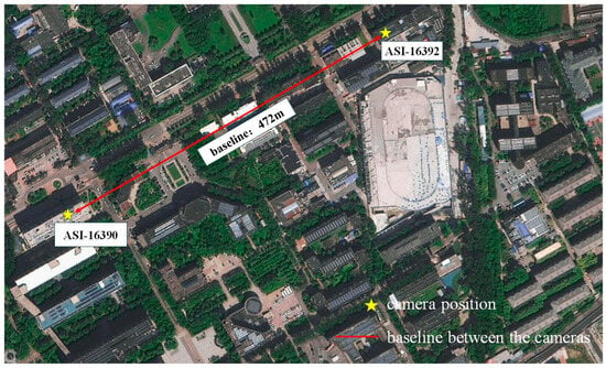
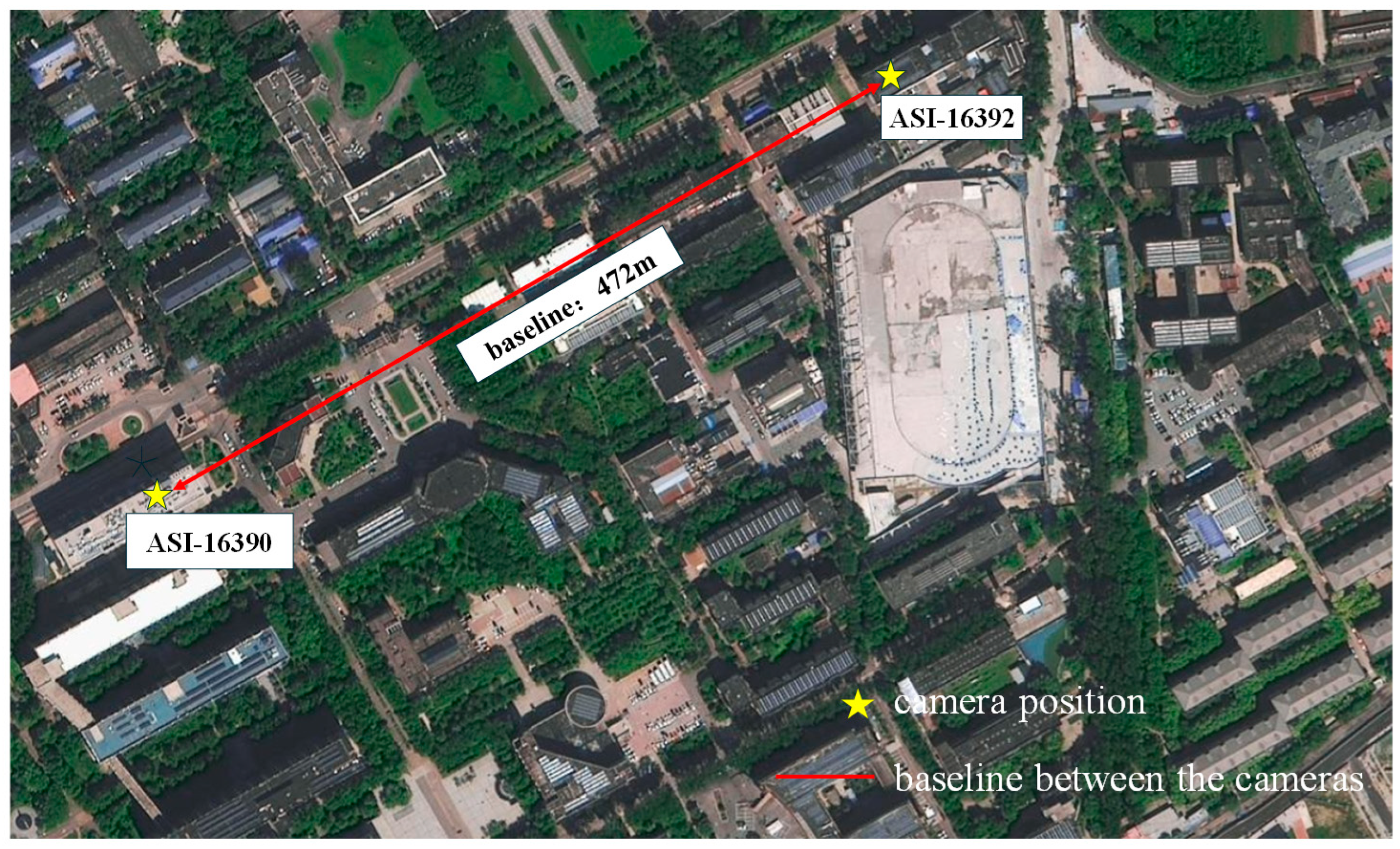
The ground-based cloud imagery utilized in this study was acquired by two EKO-ASI16 All-Sky Imagers (EKO Instruments, Tokyo, Japan, All-Sky Imager, Series Number 16) situated in Beijing, China (). The technical specifications of these instruments are detailed in Table 1. The two imagers are separated by a baseline distance of 472 m, as illustrated in Figure 1. Since their deployment in 2024, the system has continuously captured images at 30-s intervals with a resolution of 1920 × 1920 pixels. The resulting dataset encompasses a diverse range of cloud genera. For experimental consistency, the training and testing sets comprise 80,000 and 40,000 images, respectively, aligning with the structural scale of the MS-COCO dataset (Microsoft Common Objects in Context).
Table 1.
All-Sky Imager Equipment Parameters.
Figure 1.
Experimental site and Equipment.
To ensure robustness and generalizability, our methodology incorporates three distinct categories of image datasets:
Synthetic Geometric Dataset: A computer-generated dataset was constructed by stochastically rendering 2D primitives—including corners, lines, triangles, and rectangles—on solid-colored backgrounds. To enhance diversity, random affine transformations (e.g., rotation, scaling, and shearing) were applied to these primitives, providing a foundation for basic feature detection. To instill preliminary 3D spatial perception capabilities in the model from the initial training phase, we implemented a geometry-based augmentation strategy. Specifically, while generating basic 2D shapes, the system programmatically applies correlated rotations and translations to create image pairs with corresponding labels. This process effectively constructs a labeled dataset that encapsulates basic 3D geometric logic and spatial transformation consistency, enabling the model to transition from recognizing simple 2D structures to understanding simulated 3D spatial relationships before processing complex cloud imagery.
MS-COCO Public Dataset: This dataset, containing approximately 80,000 training and 40,000 testing images, covers an extensive array of natural scenes. Integrating this dataset ensures that the feature detector maintains superior generalization capabilities and avoids overfitting to specific environmental contexts.
Ground-based Cloud Imagery (GCI) Dataset: The core dataset consists of specialized cloud images. This dataset is instrumental in refining the model’s ability to extract features under the unique radiometric and morphological conditions characteristic of atmospheric clouds.
2.2. Methodology Overview
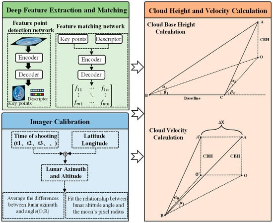
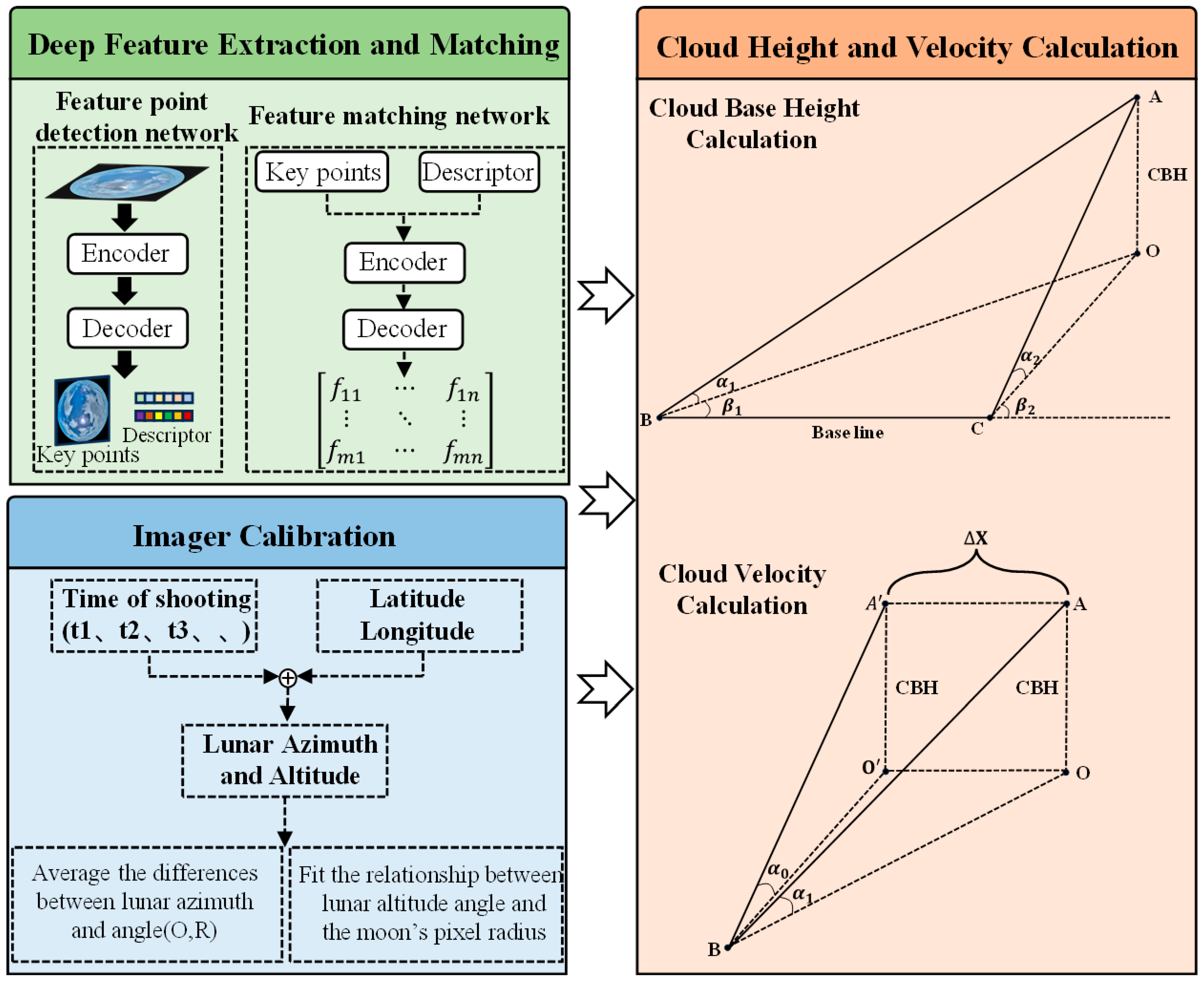
The proposed computational framework for 3D cloud velocity field estimation comprises three primary components: deep feature extraction and matching, fisheye camera calibration, and retrieval of cloud base height (CBH) and velocity. The comprehensive technical roadmap is illustrated in Figure 2.
Figure 2.
Framework for 3D cloud velocity field estimation via deep learning and binocular vision.
2.2.1. Deep Feature Extraction and Correspondence
Feature Point Extraction employs a joint learning architecture for detection and description, based on an encoder–decoder framework. The overall structure utilizes a shared feature encoder, followed by two parallel task-specific sub-networks: one for feature point localization and the other for descriptor computation [23]. The model is trained end-to-end to simultaneously optimize both tasks, thereby ensuring synergistic consistency between feature point localization and local description.
In the first phase, the model is pre-trained using the augmented synthetic geometric dataset described in Section 2.1. This “warm-up” stage focuses on establishing sensitivity to fundamental geometric edges and interest points within a simulated 3D transformation framework. By training on image pairs with predefined geometric motion, the encoder begins to internalize the spatial correspondence required for 3D analysis.
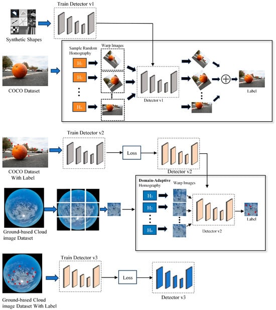
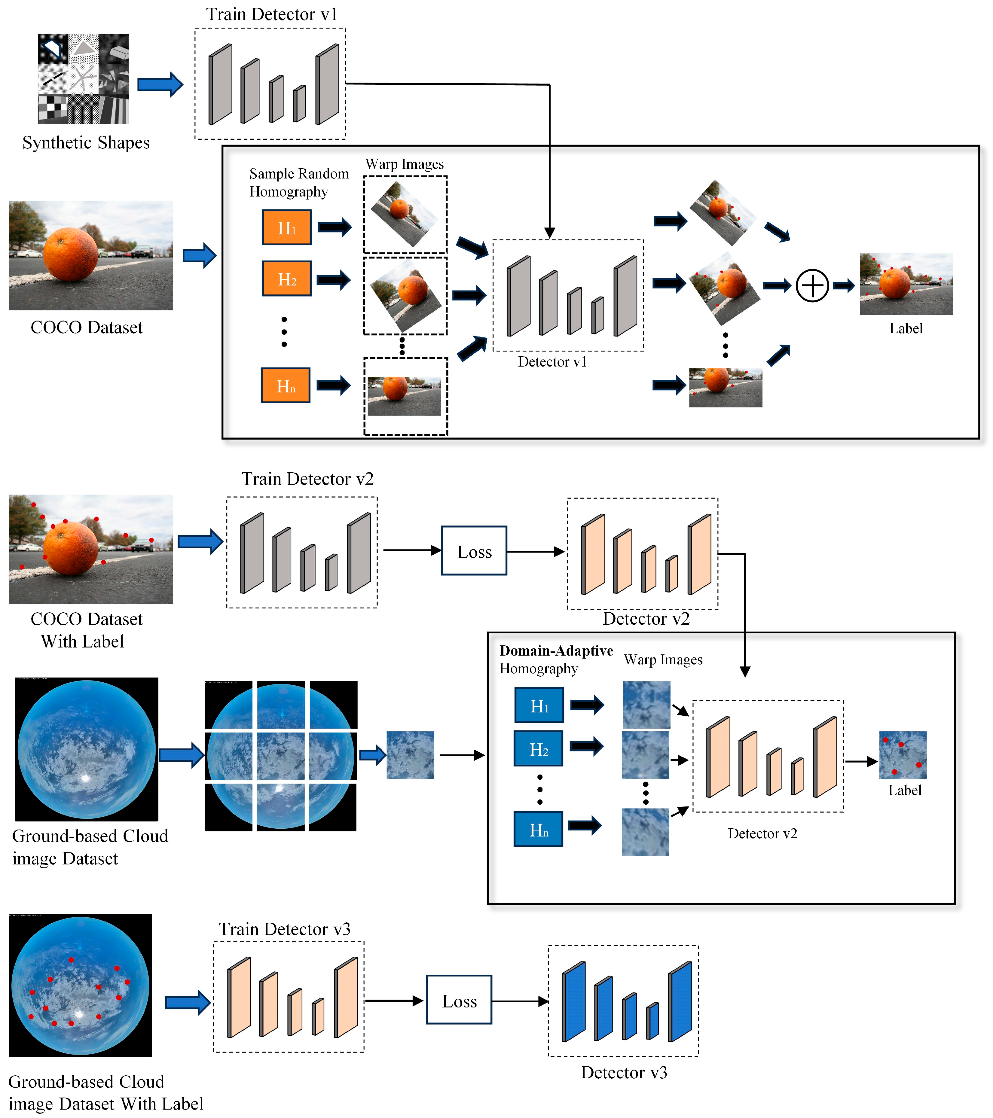
The training process adopts a “Homography Adaptation” self-supervised strategy, with key adaptations tailored to the characteristics of ground-based cloud images. The core idea of this strategy is to automatically generate pseudo keypoint labels for unlabeled real cloud images, as illustrated in Figure 3.
Figure 3.
Self-supervised training workflow for ground-based cloud feature detection.
Specifically, for an input cloud image , we first generate a sequence of N random homography transformations that conform to the physical motion patterns of cloud layer appearance. Mathematically, each transformation is represented as a 3 × 3 matrix that maps a pixel p = in the original image to a pixel in the transformed image, such that . To discuss the specific parameters, can be formulated as follows:
In this formulation, the parameters are constrained based on the specific geometry of zenith-view cloud imaging:
(1) Translation (): Unlike generic approaches, we assign the highest weight to translation, limiting the maximum shift to 30% of the image dimensions to simulate the primary horizontal drifting of clouds.
(2) Isotropic Scaling (s): The scaling factor s is constrained between 0.8 and 1.2 to simulate cloud movement toward or away from the observer (vertical velocity components or cloud growth/dissipation).
(3) In-plane Rotation (): The rotation angle is bounded within ±15° to represent slight wind-driven rotations.
(4) Perspective Distortion (): We strictly restrict these parameters (setting them near zero) to avoid severe pitch or tilt distortions, which rarely occur in natural sky scenes captured by stationary upward-looking imagers.
This biased transformation prior compels the model to focus on learning the most common and stable appearance features in cloud motion, thereby generating pseudo-labels that better align with physical reality. Subsequently, each transformation is applied to I to obtain a transformed image . An initial feature detector predicts a set of keypoints for each , which are then mapped back to the original image coordinate system via the inverse transformation to obtain pseudo-labels .
Finally, pseudo-labels generated from hundreds of random transformations are aggregated and subjected to non-maximum suppression, producing a high-quality, consistent keypoint ground-truth heatmap for the original cloud image I. This pipeline enables the model to learn the unique texture structures and appearance features of clouds directly from large-scale unlabeled ground-based cloud images, effectively mitigating the domain gap between synthetic data and real cloud imagery.
The overall loss function of the model is formulated as a weighted sum of the keypoint detection loss and the descriptor loss:
Here, represents a hyperparameter that balances the contributions of these two loss terms. We apply = 0.0001 to coordinate the detector and descriptor loss terms. This value was selected based on empirical validation across several orders of magnitude to align the scale of the cross-entropy detection loss with the high-dimensional descriptor matching loss. The use of this specific hyperparameter ensures that neither task dominates the gradient updates, thereby maintaining high localization accuracy for cloud features while achieving robust semantic description.
Here, denotes a positive pair (corresponding points), while indicates a negative pair (non-corresponding points). The terms and represent the margin boundaries for positive and negative pairs, respectively, and is the weighting factor for the positive pair loss.
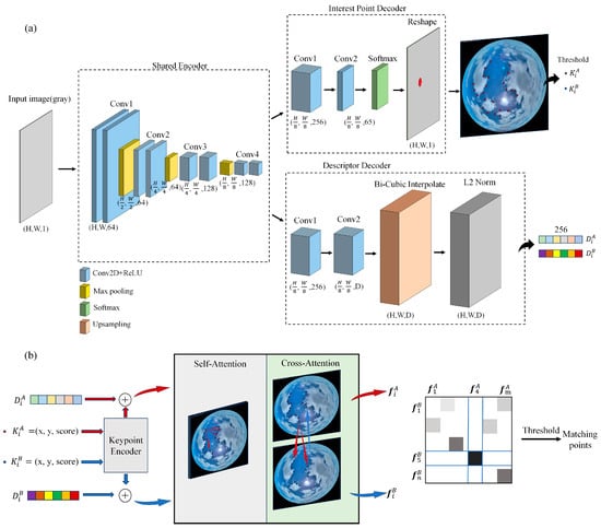
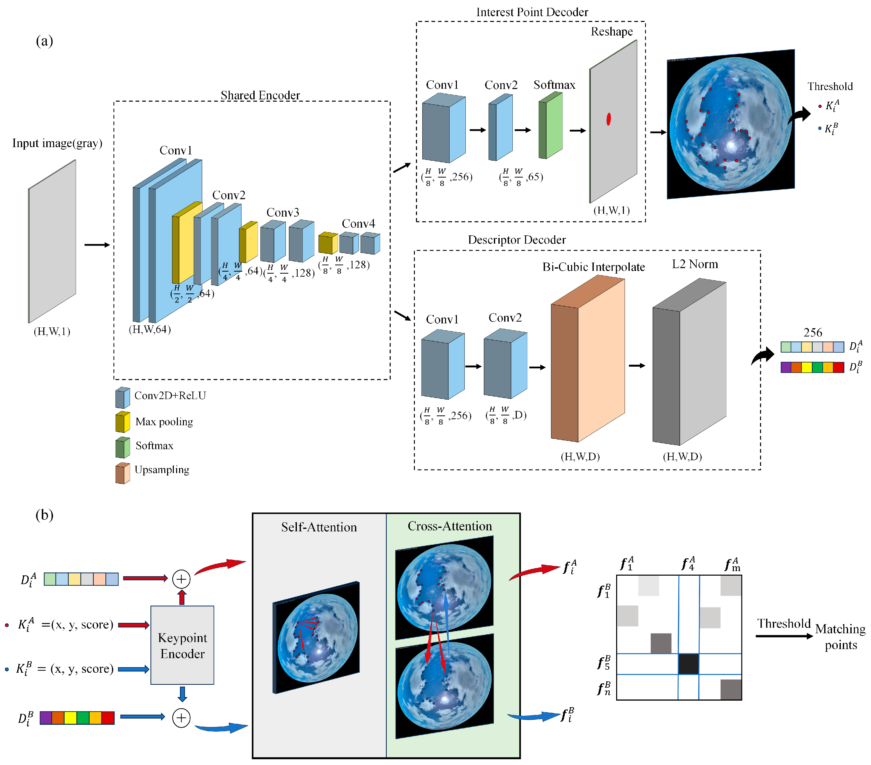
As shown in Figure 4a, an input image is first converted to grayscale with dimensions (H, W, 1). During the Encoder stage, multi-scale features are extracted through a series of convolutional layers, with three max-pooling operations progressively reducing the spatial resolution to . The resulting feature map is then fed separately into two dedicated heads: a keypoint detection head and a descriptor generation head for subsequent decoding.
Figure 4.
Deep feature perception network: (a) Shared encoder and decoder; (b) Attention-based graph matching network.
The keypoint detection head takes the encoder’s output feature map as input and processes it through two convolutional layers to produce a multi-channel response tensor with 65 channels. The first 64 channels encode the probability distribution of keypoints within each pixel cell of the encoder feature map, while the 65th channel represents the background or non-keypoint region. After applying channel-wise softmax normalization, the background channel is discarded, and the remaining 64 channels are rearranged into a 2D probability heatmap with the same resolution as the input image. Each pixel value in this heatmap indicates the confidence of being predicted as a keypoint, as illustrated in the Interest Point Decoder in Figure 4a.
Similarly, the descriptor generation head takes the encoder output and passes it through two convolutional layers to produce a dense feature map with 256 channels, corresponding to the dimensionality of the local feature vector at each cell location. This feature map is then upsampled to the original image size (H, W, D) using bicubic interpolation, where each spatial location (H, W) is associated with a 256-dimensional descriptor vector. Finally, each spatial feature vector is L2-normalized to unit length, ensuring stability in subsequent matching stages based on Euclidean distance or cosine similarity.
In terms of feature matching, we adopt the network architecture of SuperGlue [24] and incorporate a Transformer-based graph attention mechanism, which endows the matching process with global awareness and eliminates reliance on traditional nearest-neighbor search. As illustrated in Figure 4b, the model takes as input the keypoint locations, confidence scores, and corresponding descriptor vectors produced by the feature detection module. It then employs an attention-driven graph neural network to build contextualized representations for each feature. The keypoints from both images are treated as nodes in a graph, where attention mechanisms dynamically compute pairwise affinities between nodes.
A self-attention module is used to capture intra-image geometric and contextual constraints, while a cross-attention module facilitates feature interaction across the two images. Each node simultaneously attends to all nodes in the other image, thereby learning cross-image matching dependencies and enabling the model to establish a global matching context.
After nine layers of attention-based interaction, the resulting context-enhanced feature representations and are used to compute a similarity matrix , where each element represents the matching score between the -th keypoint in the first image and the -th keypoint in the second image. The similarity matrix is then normalized via Sinkhorn iteration, producing a probability distribution that approximates a doubly stochastic permutation matrix. Final correspondences are obtained by selecting the most probable matching pairs, followed by filtering based on a confidence threshold (e.g., 0.2) to reject potential outliers.
To ensure the reliability of subsequent cloud base height and velocity calculations, we implemented a two-stage abnormal matching filtering strategy to address potential mismatches during the matching process. The specific procedure is as follows:
(1) Bidirectional Consistency Verification: Based on the stereo image pairs, bidirectional feature matching is performed using both the left and right images as references. For any matching pair (A, B), if tracing back from the right image to the left image fails to return to the original point A, the match is considered inconsistent and is filtered out. This stage effectively eliminates one-way mismatches caused by ambiguous features or locally similar textures.
(2) Group Consistency Verification Based on GMS (Grid-based Motion Statistics): Considering that clouds typically move as a whole or in clusters, feature points within the same region should exhibit similar motion trends. The image is divided into uniform grids, and for any matching pair , we examine whether all matched points in the grid neighborhood of are concentrated in the corresponding neighborhood of . If the distribution of neighborhood matches is statistically significant (i.e., consistent with group motion coherence), the pair is considered a correct match; otherwise, it is filtered out. This strategy fully leverages the regional correlation of cloud motion, further enhancing the reliability of the matched set.
Through the two-stage filtering process described above, we have significantly improved the spatial consistency and physical plausibility of the matching results. This provides stable and accurate inputs for subsequent cloud height retrieval based on stereo vision and time-series velocity calculations.
2.2.2. All-Sky Imager Calibration Method
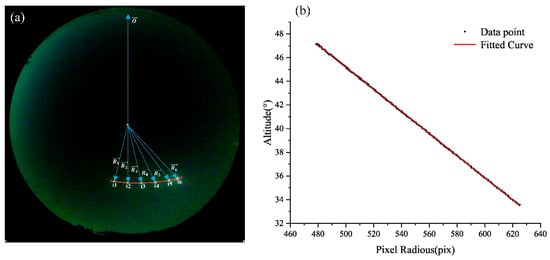
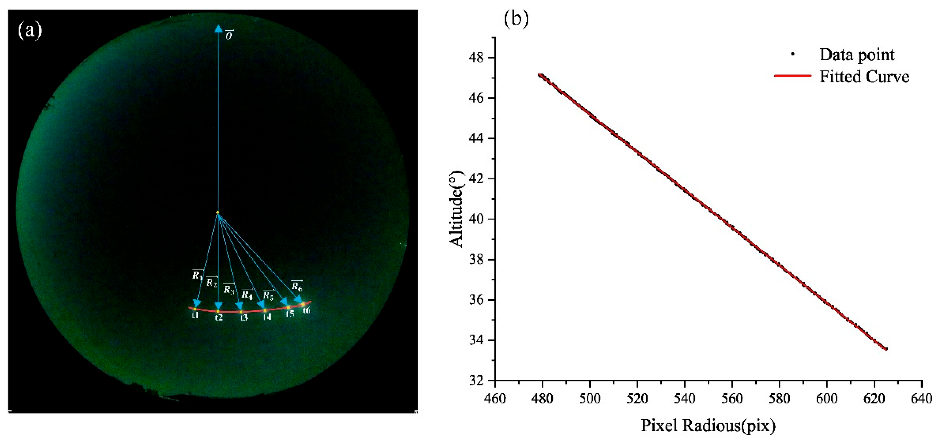
Imager calibration is the fundamental process of defining the camera’s projection function, which maps 2D pixel coordinates (x, y) to 3D celestial directions (azimuth α and altitude γ). This mapping serves as the geometric prerequisite for all subsequent physical retrievals, including Cloud Base Height (CBH) and Cloud Motion Velocity (CMV).
The design intent of using lunar observations is to utilize a high-precision celestial reference to solve the lens projection model and installation orientation bias. Unlike solar calibration, where extreme luminosity often causes “pixel blooming” and a halo effect that obscure the true solar center, the moon’s moderate brightness ensures sharp edges and stable sub-pixel centroid localization. Furthermore, at our observation site (Beijing), the moon provides a broader and more frequent range of altitude angles (12.76–90°) than the sun, ensuring a more comprehensive dataset for fitting the equidistant projection model (r = f θ).
The specific calibration procedure is illustrated in Figure 2. As shown in Figure 5a, for a lunar image captured at a known timestamp, the theoretical altitude angle is accurately determined based on the shooting time and the geographic longitude and latitude of the site. Simultaneously, the radial distance R from the lunar pixel coordinates (x, y) to the image center is calculated. By recording multiple sets of these correlated data points across various sky positions, we establish the functional relationship between the altitude angle and the pixel distance.
Figure 5.
Geometric calibration: (a) Azimuthal alignment; (b) Regression of elevation angle vs. pixel radius.
The logical connection between calibration and velocity inversion follows a rigorous pipeline:
- (1)
- Geometric Grounding: Calibration converts image displacements into angular displacements.
- (2)
- Binocular Triangulation (CBH): By combining the calibrated angles from two spatially separated imagers, we apply the principle of stereo triangulation to intersect rays in 3D space, thereby retrieving the absolute Cloud Base Height.
- (3)
- Physical Velocity Mapping (CMV): Once CBH is determined, the 2D pixel motion vectors are transformed into physical displacement vectors (in meters) using the calibrated angular scales. The 3D cloud velocity field is finally calculated by dividing these displacements by the time interval Δt.
In this study, the resulting linear fits for the altitude angle (y) and pixel distance (x) are as follows: Camera 1: , Camera 2: . These models ensure that the geometric foundation of our 3D reconstruction is both accurate and reproducible.
2.2.3. Cloud Height and Velocity Calculation Method
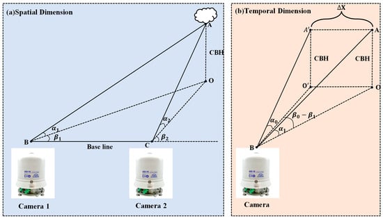
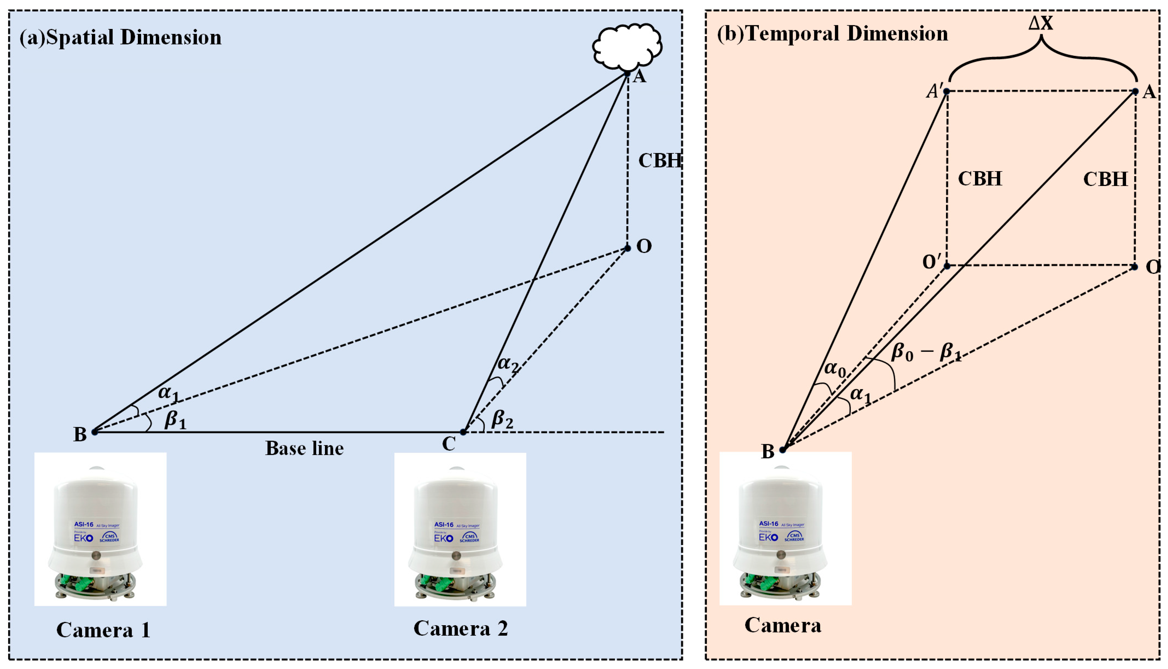
First, the cloud base height is solved stereoscopically in the spatial dimension. As shown in Figure 6a, point A represents a matched feature point output by the network from images captured simultaneously by two cameras. Based on its pixel positions in the images and the calibration results, the corresponding altitude and azimuth angles can be calculated. With the azimuth and altitude angles known, the cloud base height can then be derived using the baseline length:
where and are the altitude angles of the matched feature points in the two images, are the corresponding azimuth angles, and baseline is the distance between the two cameras, which in this experiment is set to 472 m.
Figure 6.
Cloud motion inversion: (a) Spatial binocular height estimation; (b) Temporal feature tracking for velocity.
For mixed cloud scenarios, to distinguish cloud motions at different altitudes, this study introduced a K-Means clustering algorithm based on cloud base height (CBH) for cloud layer stratification. The CBH values, retrieved through the binocular stereo vision model, were used as input features for clustering. Based on the 3σ principle, CBH outliers that significantly deviated from the overall distribution were removed. Redundant feature points in spatially adjacent areas were merged to avoid redundant calculations caused by dense textures, while sliding averaging was applied to the CBH values of the same physical points across consecutive frames to enhance temporal consistency. In this study, the number of clusters was set to K = 2, corresponding to the typical two-layer cloud structure (high cloud layer and low cloud layer). This setting was based on the analysis of a large number of measured CBH distributions and aligns with the general characteristics of two-layer clouds in meteorology. K-Means clustering was independently performed on the CBH set for each moment. To maintain temporal coherence, if the variation in the clustering center height of the same cloud layer between adjacent frames was less than 200 m, the layer was considered to have a stable and continuous height attribute. Finally, each feature point was labeled as “high-level” or “low-level” based on its assigned cluster and used for subsequent stratified velocity field calculations.
Following the stratification in the spatial dimension, feature tracking is conducted along the temporal dimension. For feature points already matched in the spatial domain, their motion across consecutive camera images is tracked. The temporal dimension calculations are built upon the spatial resolution, using the cloud base heights obtained from spatial matching as input parameters for the temporal computation, as illustrated in Figure 6b. Once all relevant parameters of the feature points are determined, their corresponding motion velocity can be calculated:
In the formula, represents the displacement of the feature point between consecutive frames, and denotes the time interval between these frames. In this experiment, the minimum time interval between consecutive frames can reach 30 s. The displacement is derived as follows:
In the formula, represents the altitude angle of the feature point in the previous frame, denotes the altitude angle in the current frame, and indicates the difference in azimuth angles between the two frames.
3. Results and Analysis
3.1. Cloud Height Calculation Validation
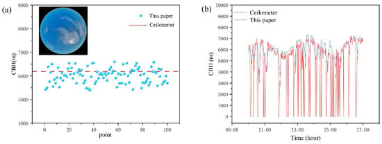
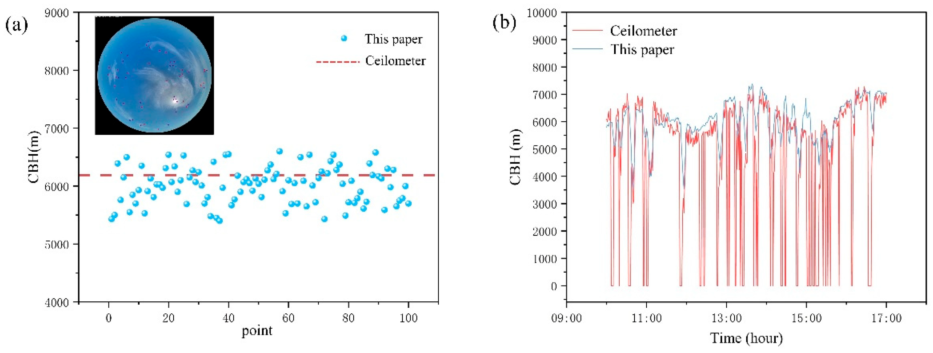
To evaluate the effectiveness of the method proposed in this study, we performed a comparative validation by comparing the calculated cloud base heights with measurements obtained from a laser ceilometer. As shown in Figure 7a, the results of cloud height estimation from a single frame are presented. For cirrus clouds, which typically have a cloud base above 5000 m, the laser ceilometer recorded an actual height of approximately 6100 m at the corresponding time. The scatter distribution of cirrus cloud heights calculated using our method shows that most results cluster around the measured value, indicating a high level of accuracy in the proposed approach.
Figure 7.
Validation against the Lidar Ceilometer: (a) Results from a single frame; (b) Results from consecutive frames.
Furthermore, we tested the performance of our method in continuous calculations, with the results illustrated in Figure 7b. It can be observed that the computational outcomes from our method align closely with the measurement trends obtained from the laser ceilometer, while maintaining a comparable level of accuracy. This consistency demonstrates the effectiveness of our approach when applied to ground-based cloud imagery.
3.2. Comparative Experiments
To thoroughly evaluate the performance of the proposed cloud motion velocity calculation method based on deep feature matching, we conducted a comparative study against two widely used classical approaches: the Scale-Invariant Feature Transform (SIFT) method and the Particle Image Velocimetry (PIV) method.
Due to the current lack of high-precision three-dimensional cloud motion ground truth data that can be directly matched with image sequences, this study did not conduct direct physical validation of the estimated cloud motion velocities. Therefore, this section compares the motion trends between the proposed method and traditional methods (SIFT, PIV) across continuous time sequences, aiming to assess their relative consistency rather than absolute physical accuracy. This approach serves as a common alternative evaluation strategy in the absence of ground truth data [13,16,25].
First, regarding feature extraction and matching capability, we adopted the following two evaluation metrics [26]:
In 3D cloud motion inversion, the spatial resolution of the resulting velocity field is highly dependent on the density of valid tracking points. Since ground-based cloud images often exhibit weak textures and diffuse boundaries, e serves as a critical measure of the model’s ability to extract sufficient landmarks in challenging regions, thereby ensuring a continuous and fine-grained velocity field.
High matching reliability is the absolute prerequisite for accurate Cloud Base Height (CBH) triangulation. By utilizing m, we can effectively filter out unstable or ambiguous matches caused by cloud deformation and perspective changes, ensuring that the retrieved 3D motion vectors remain physically and logically consistent.
In the formula, represents the feature extraction capability of the method used, where corresponds to the total number of feature points extracted by the SIFT method, and denotes the total number of feature points extracted by the evaluated method. A larger value of indicates a richer set of potential candidates for subsequent motion calculation and better spatial coverage.
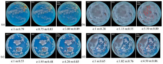
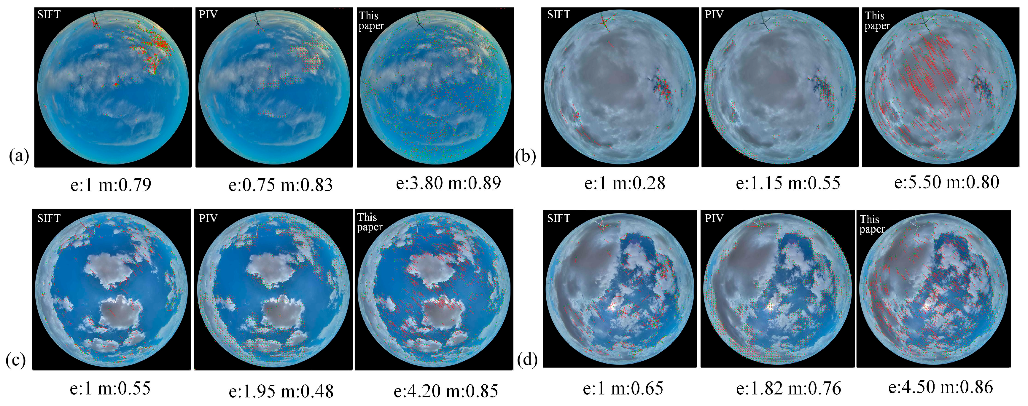
Figure 8 visually illustrates the performance of the three methods on different types of cloud images. It can be observed that the SIFT method tends to concentrate feature points in local regions with dense textures. The PIV method demonstrates a certain ability to capture global motion and extracts cloud motion in some areas; however, it performs poorly in stratiform clouds with weak texture features. In contrast, the proposed method achieves consistently better results across various cloud types.
Figure 8.
Performance of the three methods on different cloud types. (a) Cirrus; (b) Stratus; (c) Cumulus; (d) Mixed clouds.
Table 2 presents the computational results of the four methods across different types of cloud images. It can be observed that the proposed method, leveraging its self-supervised feature extraction network, demonstrates a clear advantage over the others across all cloud types. On average, its feature extraction capability reaches 4.5 times that of the SIFT method. Notably, for texture-sparse stratiform clouds, our approach effectively captures weak texture features that are difficult for traditional methods to detect, thereby providing a more substantial data foundation for subsequent calculations.
Table 2.
Comparison of feature extraction capability (e) and feature matching quality (m) for the three methods. (Bold values indicate the best performance for each metric).
We further applied the four methods to a continuous cloud motion velocity time series to evaluate the performance of the proposed method over an extended temporal scale. A cumulus cloud motion dataset spanning 80 min was selected for this analysis. To establish a more reliable baseline for comparison, the average results of the two traditional methods—SIFT and PIV—were used as the reference model.
Note that the traditional methods (SIFT and PIV) compute velocity in units of pixels per second (pix/s), whereas the proposed method estimates the actual physical cloud motion velocity in meters per second (m/s). To objectively compare the performance across methods, we employed the Pearson correlation coefficient to measure the correlation between the results of each method and the baseline outcomes:
where and represent the mean values of datasets X and Y, respectively. The computed results are presented in Table 3. The proposed method achieved the highest Pearson correlation coefficient (r = 0.662), indicating stronger relative consistency in motion trends with the benchmark model, rather than representing the absolute accuracy of physical velocities.
Table 3.
Results of Pearson Correlation Analysis. (Bold values indicate the best performance for each metric).
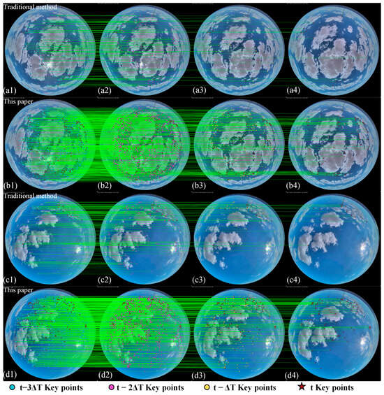
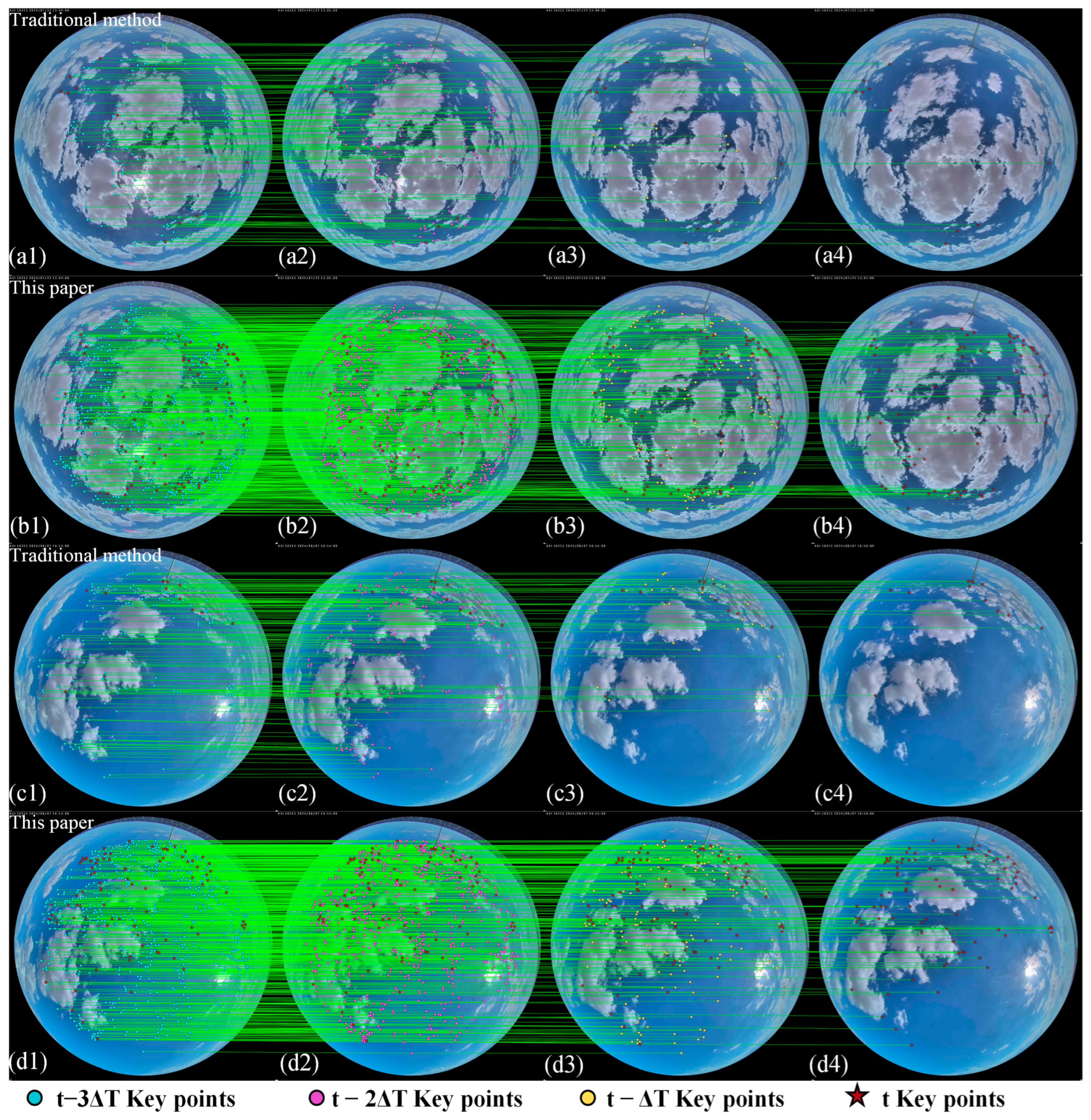
To further evaluate the long-term stability of this method in tracking cloud feature points across continuous time sequences, we conducted a multi-frame tracking experiment under a single-camera perspective. The experiment selected a continuous image sequence (t, t − ΔT, t − 2ΔT, t − 3ΔT) to persistently track the continuous presence of feature points.
To quantify the tracking capability, we introduce the Feature Point Retention Rate (FPR) as an evaluation metric. It is defined as the percentage of feature points initially detected in the starting frame that are still successfully matched and tracked in the third subsequent frame (i.e., at ), relative to the total number of initial feature points. This metric effectively reflects the algorithm’s robustness to changes in cloud appearance. The specific formula is as follows:
Among these, represents the feature points matched at the current moment, while represents the feature points that remain continuously detected and matched over the subsequent time interval. As shown in Figure 9, the feature tracking capabilities of the proposed method and the traditional method are compared. In the figure, the red five-pointed stars indicate the feature points that persist across multiple frames, which are subsequently used as inputs for cloud height and velocity calculations.
Figure 9.
Comparison of Feature Tracking Capabilities Between the Traditional Method and the Proposed Method in Single-Camera Continuous Time Frames. (a1–a4) Feature tracking results of the traditional method applied to the first cloud image sequence at time steps , , , and , respectively. (b1–b4) Feature tracking results of the proposed method applied to the same cloud image sequence as in (a), showing the tracking performance at , , , and . (c1–c4) Feature tracking results of the traditional method applied to the second cloud image sequence at time steps , , , and . (d1–d4) Feature tracking results of the proposed method applied to the same cloud image sequence as in (c) at , , , and . The colored markers (blue, purple, yellow circles, and red stars) indicate keypoints at different historical and current time steps, and the green lines represent the matching trajectories.
As shown in Table 4, the proposed method extracts a significantly higher number of feature points in the initial frame compared to the traditional method—approximately four times as many—providing a richer candidate feature set for subsequent temporal tracking. After cloud movement and deformation over two frames (60 s), the feature point retention rate of the traditional method is extremely low (approximately 5–6%), indicating that its descriptors are highly sensitive to the non-rigid deformation of clouds and struggle to maintain long-term matches. In contrast, after the same time interval, the proposed method maintains a feature point retention rate above 10%, demonstrating the advantage of the graph attention-based matching mechanism in modeling long-range dependencies and contextual information, which enables more robust handling of continuous changes in cloud texture. A higher feature point retention rate means longer and more coherent motion trajectories can be constructed in continuous time series. This directly improves the reliability and smoothness of estimating the instantaneous velocity from displacement , effectively reducing motion estimation noise caused by frequent feature point loss and re-detection. This provides a key guarantee for retrieving stable and continuous 3D cloud motion velocity fields from image sequences.
Table 4.
Feature Point Retention Rate (FPR) for the Traditional Method and the Proposed Method. (Bold values indicate the best performance for each metric).
3.3. Results Across Multiple Cloud Types
We conducted systematic experiments on four typical cloud types (cirrus, cumulus, stratus, and mixed clouds). First, cloud base height (CBH) data for each cloud sample were obtained using a binocular image-based CBH inversion model. Subsequently, through feature matching and motion estimation across consecutive temporal frames, dynamic tracking of cloud motion was achieved in both spatial and temporal dimensions. This process integrates CBH information, enabling accurate characterization of the three-dimensional features of cloud motion.
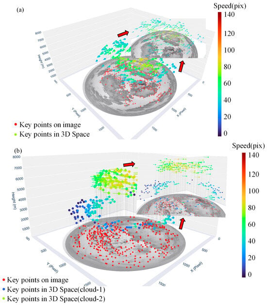
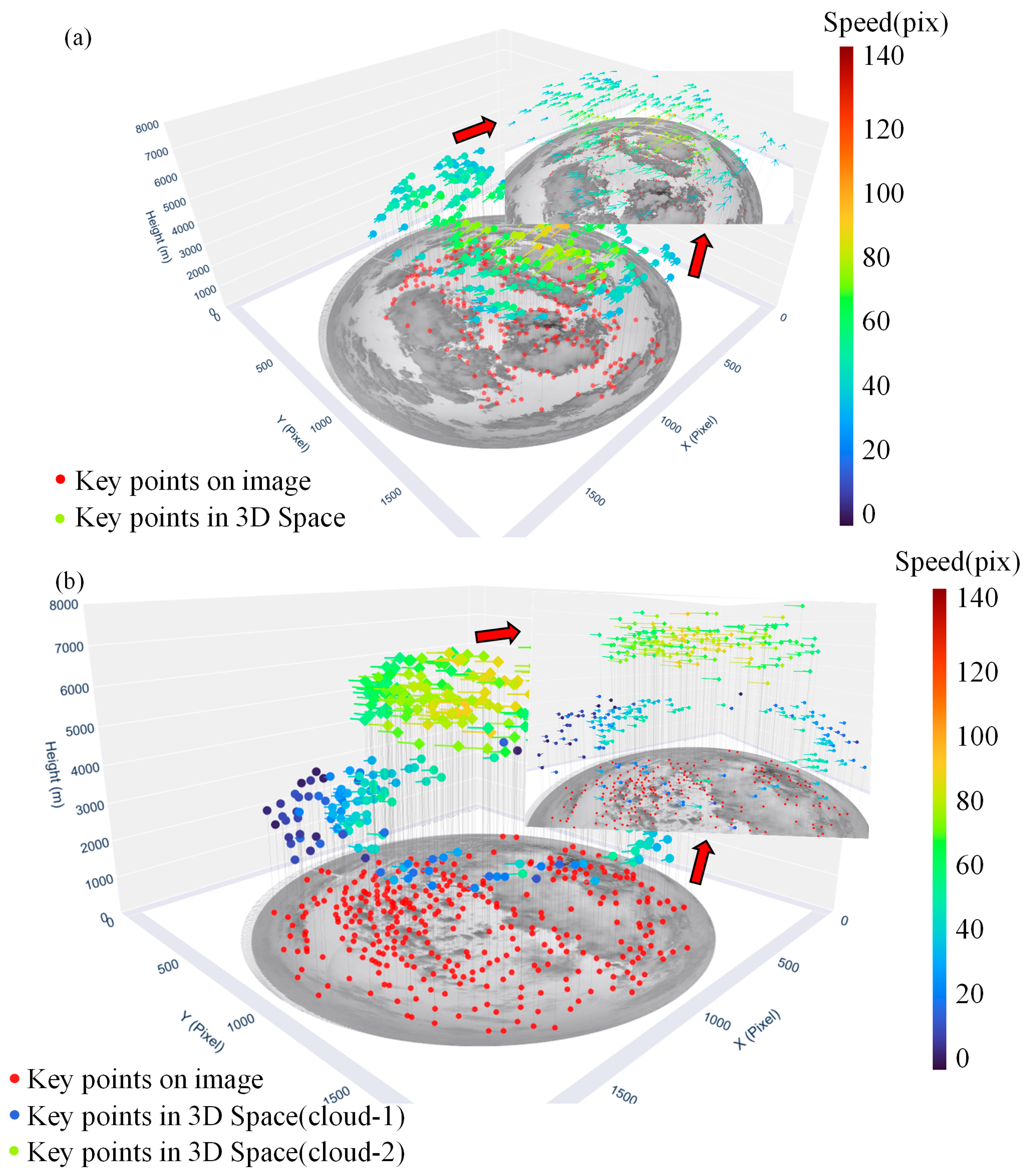
As shown in Figure 10, the proposed method demonstrates robust feature retention capability and motion consistency across various cloud-type scenarios. For single-layer clouds, despite their coarse texture and significant local deformation, the algorithm maintains high matching accuracy even under strong brightness variations and local shadow interference, thanks to the densely distributed feature points. In mixed cloud scenarios, the CBH-based K-Means clustering stratification method employed reveals that the proposed approach can effectively distinguish the motion states of cloud masses at different altitude layers (Figure 10b). The separated high- and low-layer clouds exhibit clear and independent motion trajectories in three-dimensional space, demonstrating the method’s effectiveness and adaptability in parsing complex multi-layer cloud structures.
Figure 10.
3D dynamic velocity field visualization for typical cloud types. (a) single-layer cloud. (b) Mixed-cloud.
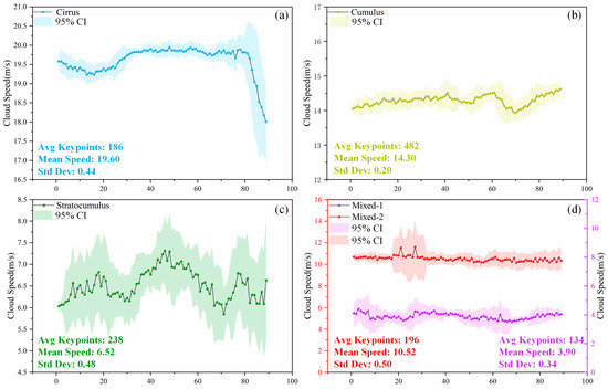
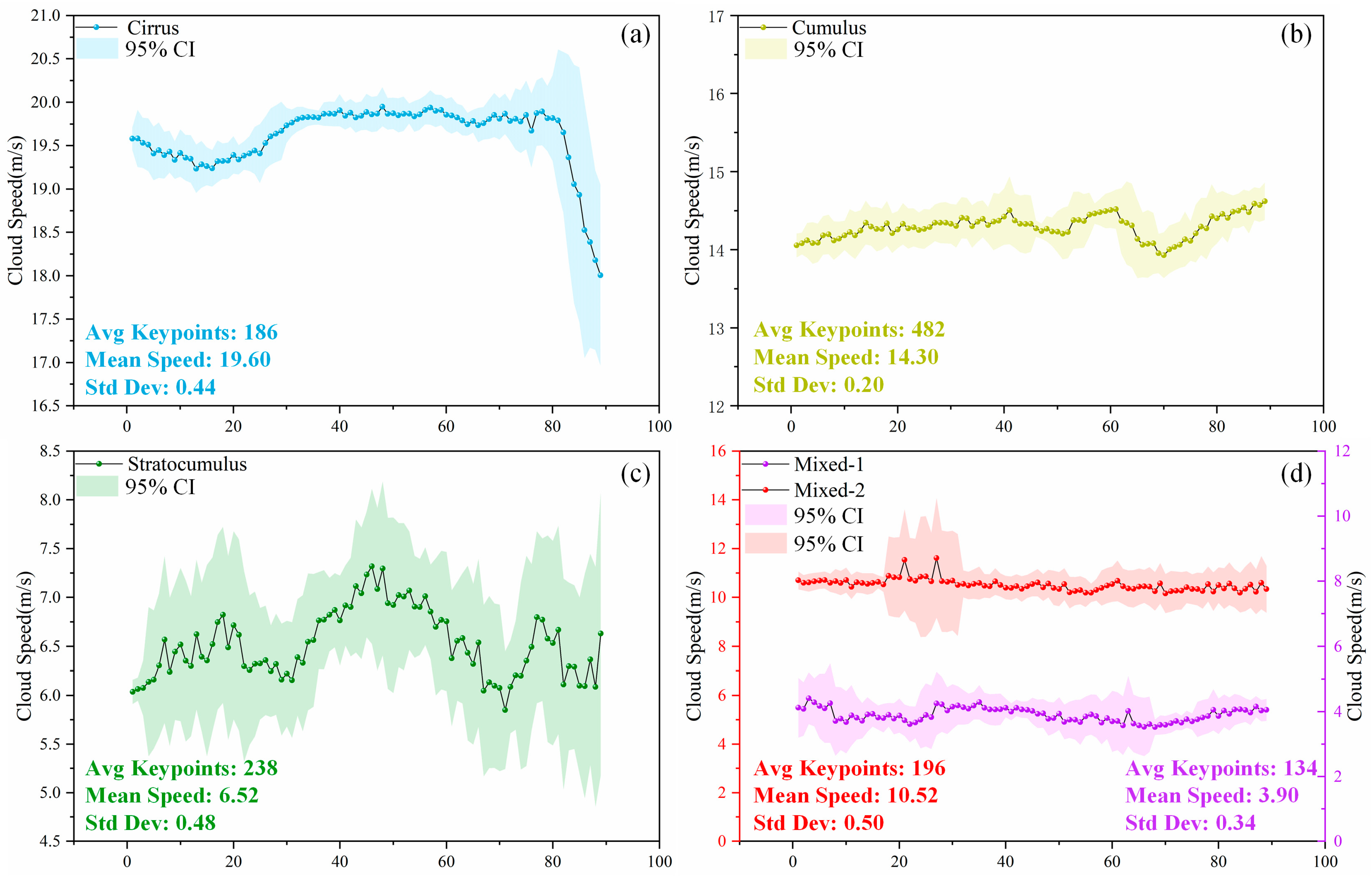
Furthermore, Figure 11 illustrates the continuous temporal variation in cloud motion velocities for the four cloud types during the experiment, accompanied by statistical indicators such as average keypoint count, mean velocity, and standard deviation. The results indicate that the motion characteristics of different cloud types are closely correlated with their physical properties and atmospheric altitudes. Cirrus clouds (Figure 11a), which are high-altitude clouds, exhibited the highest velocities, averaging 19.60 m/s with a low standard deviation of 0.44 m/s. This reflects their stable, large-scale circulation driven by high-altitude wind belts. The algorithm tracked an average of 186 keypoints, with a sharp decline around 80 min, consistently corresponding to the cirrus layer moving out of the field of view. Cumulus clouds (Figure 11b) showed an average speed of 14.30 m/s and the highest tracking density, with 482 average keypoints. The stability of their velocity curve, indicated by a standard deviation of 0.20 m/s, aligns with the moderate and steady wind speeds driven by local thermal convection in mid-to-low-level clouds. In the case of stratocumulus clouds (Figure 11c), the updated analysis reveals an average speed of 6.52 m/s. Despite the relatively slow horizontal drift under stable atmospheric stratification, their velocity fluctuations were more pronounced, with a standard deviation of 0.48 m/s compared to cumulus clouds. For mixed clouds (Figure 11d), the two-layer structure is clearly distinguishable. The higher-layer component (Mixed-2) recorded an average speed of 10.52 m/s, while the lower-layer component (Mixed-1) showed an average speed of only 3.90 m/s. The distinct differences in velocity and the number of tracked keypoints (196 for Mixed-2 versus 134 for Mixed-1) demonstrate the superior capability of the proposed framework in resolving multi-layer atmospheric dynamics.
Figure 11.
Continuous velocity evolution of cloud clusters at different altitudes during the observation period. (a) Cirrus (b) Cumulus (c) Stratocumulus (d) Mixed.
3.4. Uncertainty Propagation and Efficacy Analysis
To evaluate the instrumental and algorithmic efficacy of the 3D cloud motion inversion, this section quantifies how uncertainties in observational variables propagate to the final velocity estimates.
According to the binocular geometric model established in this paper, the inversion accuracy of cloud velocity (v) is primarily governed by the calculation of cloud base height (H) and the tracking precision of feature points across time series. All random errors associated with the observations have been uniformly mapped to the fundamental pixel-matching uncertainty (σp).
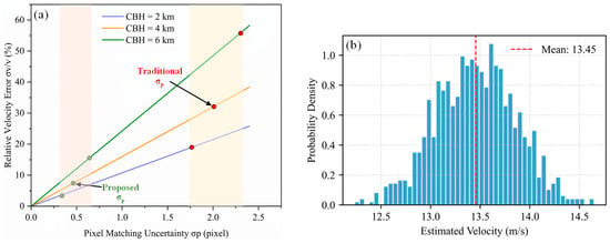
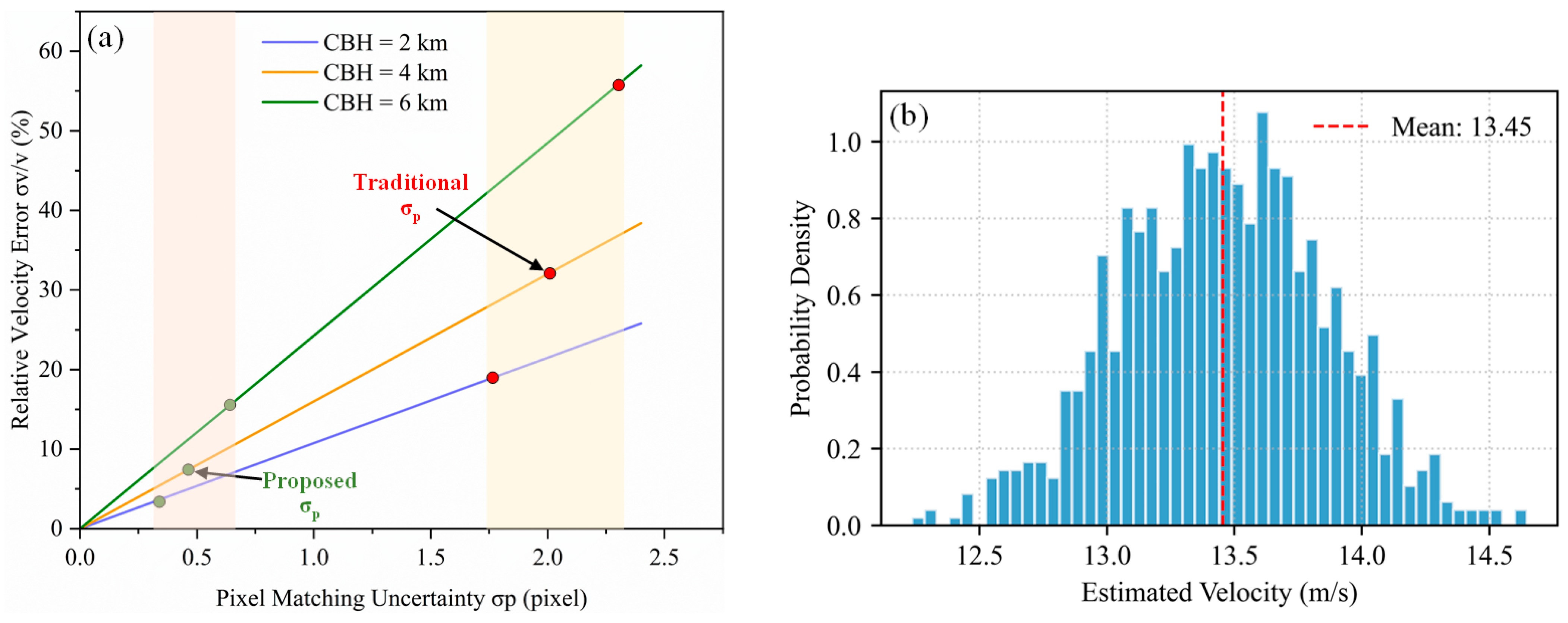
As shown in Figure 12a, the relative velocity error σv/v exhibits a linear increase with the growth of pixel error σp, a trend that is simultaneously influenced by the cloud base height H. We computed the σp values for both the conventional method and the proposed method under three different cloud height types. The results indicate that the matching error of the conventional method typically ranges between 1.5 and 2.5 pixels. In contrast, by employing a self-supervised feature extraction and matching mechanism, the proposed method consistently maintains σp around 0.5 pixels. This effectively constrains the associated error below 15%, thereby ensuring the validity of the inversion results.
Figure 12.
Error Analysis within the 3D Inversion Framework. (a) Sensitivity analysis of relative velocity error to pixel-matching uncertainty under different cloud base heights (H). (b) Probability density distribution of cloud velocity estimates from Monte Carlo simulations under 0.1° noise.
Given the nonlinear characteristics inherent in the trigonometric relationships of the cloud velocity calculation principle, we further introduced Monte Carlo simulation (N = 1000) to verify the system’s robustness under random noise. We simulated a standard mid-level cloud observation scenario and introduced Gaussian angular noise with a standard deviation of 0.1° to comprehensively account for instrumental errors and pixel-matching inaccuracies. The resulting probability density distribution of the simulated cloud velocities is presented in Figure 12b. The results show that the estimated cloud velocity has a mean error of 13.45 m/s with a standard deviation of 0.40 m/s. This compact distribution demonstrates that, although the 3D inversion is sensitive to angles, the errors remain convergent within the precision afforded by our framework. The 95% confidence interval [12.65, 14.23] lies within a physically plausible range, with no outlier divergence observed. This confirms that the strategy of improving feature-matching accuracy to compensate for inherent instrumental observational fluctuations is effective for 3D cloud motion inversion.
4. Conclusions
In this paper, we propose a cloud motion velocity field estimation method that integrates binocular camera imaging with self-supervised deep feature learning. This approach effectively addresses the limitations of traditional cloud motion estimation techniques, such as unstable feature extraction under complex cloud conditions, low matching accuracy, and the lack of physical dimensional information. By introducing a self-supervised feature point detection framework tailored for ground-based cloud images and a graph attention-based feature matching mechanism, our method significantly improves the ability to perceive and track cloud features in scenarios involving cloud deformation, weak-texture regions, and non-linear motion.
Experimental results demonstrate that the proposed method exhibits strong robustness and accuracy across multiple typical cloud types—cirrus, cumulus, stratus, and mixed clouds. In terms of feature extraction capability, it achieves an average of 4.5 times the number of features extracted by the conventional SIFT method. When evaluated on continuous time-series data, the Pearson correlation coefficient with the baseline model reaches 0.662, outperforming all compared methods. Furthermore, comparisons with laser ceilometer measurements validate the effectiveness and reliability of our approach in both cloud height retrieval and motion velocity calculation.
Future work will focus on exploring multi-scale cloud motion modeling, cross-modal data fusion (e.g., integrating meteorological radar and satellite data), and assessing the practical deployment performance of the method in photovoltaic power forecasting systems.
It should be noted that due to the lack of directly verifiable ground truth data for cloud motion velocity, the performance evaluation in this study primarily relies on comparative correlation analysis with traditional methods, emphasizing the relative consistency of motion trends. In the future, the accuracy of physical velocities will be further validated through multi-source data fusion, such as integrating wind profiler radar and meteorological radar observations.
Author Contributions
Conceptualization, S.J.; Methodology, S.J. and X.F.; Software, S.J., X.F. and L.L.; Validation, S.J. and L.L.; Formal analysis, S.J.; Investigation, S.J.; Resources, C.Z., X.F. and Z.W.; Data curation, C.Z., L.L. and Z.W.; Writing—original draft, C.Z. and L.L.; Writing—review & editing, C.Z.; Supervision, C.Z., X.F., Z.W., X.L. and J.S.; Project administration, C.Z. and X.L.; Funding acquisition, T.L. All authors have read and agreed to the published version of the manuscript.
Funding
This work was supported by the Science and Technology Project of China Power Engineering Consulting Group Co., LTD.: “Research and Application of Key Technologies for Intelligent Control and Operation Improvement of ‘CSP+’ Power Plants” (Grant No. DG2-K01-2024).
Institutional Review Board Statement
Not applicable.
Informed Consent Statement
Not applicable.
Data Availability Statement
The original contributions presented in this study are included in the article. Further inquiries can be directed to the corresponding authors.
Acknowledgments
The authors would like to express their gratitude to the technical staff at the China Power Engineering Consulting Group for their assistance in the deployment of the All-Sky Imagers and data collection at the experimental site in Beijing. We also thank the anonymous reviewers for their constructive comments that helped improve the quality of this manuscript.
Conflicts of Interest
Authors Shan Jiang, Zhikuan Wang, Xingtong Li and Tianying Liu were employed by the China Power Construction Engineering Consulting Corporation. Authors Chen Zhang and Xu Fu were employed by the China Power Engineering Consulting Group Co., LTD. Author Lei Lin was employed by the East China Electric Power Design Institute Co., LTD. of China Power Engineering Consulting Corporation. The remaining authors declare that the research was conducted in the absence of any commercial or financial relationships that could be construed as a potential conflict of interest.
Abbreviations
| CBH | Cloud Base Height |
| PV | Photovoltaic |
| LIDAR | Light Detection and Ranging |
| RADAR | Radio Detection and Ranging |
| GCI | Ground-based cloud images |
| ASI | All-Sky Imagers |
| VOF | Variational Optical Flow |
| CCLSTM-SR-Net | Channel-wise Correlation LSTM-Super-Resolution Network |
| GRU-RCN | Gated Recurrent Unit-Recurrent Convolutional Network |
| FPCT | Fourier Phase Correlation Theory |
| CMV | Cloud Motion Vector |
| GNN | Graph neural network |
| MS-COCO | Microsoft Common Objects in Context |
| FOV | Field of View |
| RGB | Red Green Blue |
| H, W, D | Height, Width, Depth |
| PIV | Particle Image Velocimetry |
| SIFT | Scale-Invariant Feature Transform |
References
- Chow, C.W.; Belongie, S.; Kleissl, J. Cloud motion and stability estimation for intra-hour solar forecasting. Sol. Energy 2015, 115, 645–655. [Google Scholar] [CrossRef] [Scilit]
- Chu, D. Accuracy Assessment of NOAA IMS 4 km Products on the Tibetan Plateau with Landsat-8 OLI Images. Atmosphere 2024, 15, 1234. [Google Scholar] [CrossRef] [Scilit]
- Gyasi, E.K.; Swarnalatha, P. Cloud-MobiNet: An Abridged Mobile-Net Convolutional Neural Network Model for Ground-Based Cloud Classification. Atmosphere 2023, 14, 280. [Google Scholar] [CrossRef] [Scilit]
- Zekoll, V.; de los Reyes, R.; Richter, R. A Newly Developed Algorithm for Cloud Shadow Detection—TIP Method. Remote Sens. 2022, 14, 2922. [Google Scholar] [CrossRef] [Scilit]
- Hu, F.; Hou, B.; Zhu, W.; Zhu, Y.; Zhang, Q. CloudY-Net: A Deep Convolutional Neural Network Architecture for Joint Segmentation and Classification of Ground-Based Cloud Images. Atmosphere 2023, 14, 1405. [Google Scholar] [CrossRef] [Scilit]
- Travieso-González, C.M.; Cabrera-Quintero, F.; Piñán-Roescher, A.; Celada-Bernal, S. A Review and Evaluation of the State of Art in Image-Based Solar Energy Forecasting: The Methodology and Technology Used. Appl. Sci. 2024, 14, 5605. [Google Scholar] [CrossRef] [Scilit]
- Zhang, Y.; Cao, D.; Yang, J.; Lu, F.; Wang, D.; Liu, R.; Zhang, H.; Liu, D.; Chen, Z.; Lyu, H.; et al. A Parallax Shift Effect Correction Based on Cloud Top Height for FY-4A Lightning Mapping Imager (LMI). Remote Sens. 2023, 15, 4856. [Google Scholar] [CrossRef] [Scilit]
- Zhen, Z.; Liu, J.; Zhang, Z.; Wang, F.; Chai, H.; Yu, Y.; Lu, X.; Wang, T.; Lin, Y. Deep Learning Based Surface Irradiance Mapping Model for Solar PV Power Forecasting Using Sky Image. IEEE Trans. Ind. Appl. 2020, 56, 3385–3396. [Google Scholar] [CrossRef] [Scilit]
- Park, S.; Kim, Y.; Ferrier, N.J.; Collis, S.M.; Sankaran, R.; Beckman, P.H. Prediction of Solar Irradiance and Photovoltaic Solar Energy Product Based on Cloud Coverage Estimation Using Machine Learning Methods. Atmosphere 2021, 12, 395. [Google Scholar] [CrossRef] [Scilit]
- He, M.; Zhang, J.; He, Y.; Zuo, X.; Gao, Z. Annotated Dataset for Training Cloud Segmentation Neural Networks Using High-Resolution Satellite Remote Sensing Imagery. Remote Sens. 2024, 16, 3682. [Google Scholar] [CrossRef] [Scilit]
- Ye, T.; Tan, Z.; Ai, W.; Ma, S.; Zhao, X.; Hu, S.; Liu, C.; Guo, J. On the Hybrid Algorithm for Retrieving Day and Night Cloud Base Height from Geostationary Satellite Observations. Remote Sens. 2025, 17, 2469. [Google Scholar] [CrossRef] [Scilit]
- Wang, Z.; Zhao, L.; Meng, J.; Han, Y.; Li, X.; Jiang, R.; Chen, J.; Li, H. Deep Learning-Based Cloud Detection for Optical Remote Sensing Images: A Survey. Remote Sens. 2024, 16, 4583. [Google Scholar] [CrossRef] [Scilit]
- Aicardi, D.; Musé, P.; Alonso-Suárez, R. A comparison of satellite cloud motion vectors techniques to forecast intra-day hourly solar global horizontal irradiation. Sol. Energy 2022, 233, 46–60. [Google Scholar] [CrossRef] [Scilit]
- Dissawa, D.M.L.H.; Godaliyadda, G.M.R.I.; Ekanayake, M.P.B.; Ekanayake, J.B.; Agalgaonkar, A.P. Cross-correlation based cloud motion estimation for short-term solar irradiation predictions. In Proceedings of the 2017 IEEE International Conference on Industrial and Information Systems (ICIIS), Peradeniya, Sri Lanka, 15–16 December 2017; pp. 1–6. [Google Scholar]
- Li, M.; Chu, Y.; Pedro, H.T.C.; Coimbra, C.F.M. Quantitative evaluation of the impact of cloud transmittance and cloud velocity on the accuracy of short-term DNI forecasts. Renew. Energy 2016, 86, 1362–1371. [Google Scholar] [CrossRef] [Scilit]
- Wang, F.; Zhen, Z.; Liu, C.; Mi, Z.Q.; Hodge, S.M.; Shafie-khah, M.; Catalao, J.P.S. Image phase shift invariance based cloud motion displacement vector calculation method for ultra-short-term solar PV power forecasting. Energy Convers. Manag. 2018, 157, 123–135. [Google Scholar] [CrossRef] [Scilit]
- Li, S.; Wang, M.; Shi, M.; Wang, J.; Cao, R. Leveraging Deep Spatiotemporal Sequence Prediction Network with Self-Attention for Ground-Based Cloud Dynamics Forecasting. Remote Sens. 2025, 17, 18. [Google Scholar] [CrossRef] [Scilit]
- Ansong, M.; Huang, G.; Nyang’onda, T.N.; Musembi, R.J.; Richards, B.S. Very short-term solar irradiance forecasting based on open-source low-cost sky imager and hybrid deep-learning techniques. Sol. Energy 2025, 294, 113516. [Google Scholar] [CrossRef] [Scilit]
- Su, X.Y.; Li, T.J.; An, C.; Wang, G.Q. Prediction of Short-Time Cloud Motion Using a Deep-Learning Model. Atmosphere 2020, 11, 1151. [Google Scholar] [CrossRef] [Scilit]
- Lu, Z.Y.; Wang, Z.H.; Li, X.; Zhang, J.F. A Method of Ground-Based Cloud Motion Predict: CCLSTM plus SR-Net. Remote Sens. 2021, 13, 3876. [Google Scholar] [CrossRef] [Scilit]
- Beekmans, C.; Schween, J.; Lennefer, M.; Simmer, C. Comparison of Cloud Motion Vector Profile Derived from Ground-Based Hemispheric Stereocameras to Wind-Lidar Observations. Meteorol. Z. 2021, 30, 503–513. [Google Scholar] [CrossRef] [Scilit]
- Kosmopoulos, P.; Dhake, H.; Melita, N.; Tagarakis, K.; Georgakis, A.; Stefas, A.; Vaggelis, O.; Korre, V.; Kashyap, Y. Multi-Layer Cloud Motion Vector Forecasting for Solar Energy Applications. Appl. Energy 2024, 353, 122144. [Google Scholar] [CrossRef] [Scilit]
- DeTone, D.; Malisiewicz, T.; Rabinovich, A. SuperPoint: Self-Supervised Interest Point Detection and Description. arXiv 2017, arXiv:1712.07629v4. [Google Scholar]
- Sarlin, P.-E.; DeTone, D.; Malisiewicz, T.; Rabinovich, A. SuperGlue: Learning Feature Matching with Graph Neural Networks. arXiv 2019, arXiv:1911.11763. [Google Scholar]
- Wei, L.; Zhu, T.T.; Guo, Y.R.; Ni, C.; Zheng, Q.Y. CloudpredNet: An Ultra-Short-Term Movement Prediction Model for Ground-Based Cloud Image. IEEE Access 2023, 11, 97177–97188. [Google Scholar] [CrossRef] [Scilit]
- Zou, L.L.; Tang, P.; Niu, Y.S.; Yan, Z.X.; Lin, X.L.; Song, J.F.; Wang, Q. A Cloud Motion Estimation Method Based on Cloud Image Depth Feature Matching. IEEE Geosci. Remote Sens. Lett. 2025, 22, 1000105. [Google Scholar] [CrossRef] [Scilit]

Disclaimer/Publisher’s Note: The statements, opinions and data contained in all publications are solely those of the individual author(s) and contributor(s) and not of MDPI and/or the editor(s). MDPI and/or the editor(s) disclaim responsibility for any injury to people or property resulting from any ideas, methods, instructions or products referred to in the content. |
© 2026 by the authors. Licensee MDPI, Basel, Switzerland. This article is an open access article distributed under the terms and conditions of the Creative Commons Attribution (CC BY) license.