HF Lightning Observations in the Upper Volga Region of Russia

Abstract

Much of the information for studying the processes of lightning discharge initiation and development is provided by studying thundercloud radio emissions in various frequency bands. The High-Frequency (HF) band better corresponds to the characteristic scales of lightning development but has been undeservedly forgotten and is used quite rarely. Based on observations carried out in the Upper Volga region it is shown that the intensity of HF radio emissions from lightning is high enough to be reliably recorded in nearby thunderstorms. It is found that at all stages of lightning development the intensity of its radio emission in the HF band up to 10 MHz exceeds the average background intensity significantly. The amplitudes of lightning pulses exceed the background level more significantly, up to 60 dB and more. The feasibility of using the HF band for lightning observations including tracing the direction of arrival of a radio emission is clearly demonstrated.

1. Introduction

Monitoring thunderstorm activity, particularly cloud-to-ground lightning discharges, is of significant interest from both a scientific and practical perspective. Although the study of lightning as an electrical discharge between a thundercloud and the ground began several centuries ago, a complete understanding of its nature remains elusive. Specifically, the mechanism for initiating lightning, which occurs in electric fields much lower than the threshold fields for conventional breakdown, remains unclear. In practical terms, lightning, as a hazardous natural phenomenon, causes significant damage to economic activity and even poses a threat to human life. The negative consequences of lightning strikes can be significantly reduced by predicting the location and time of a strike in advance, even at short notice.

Much of the information for studying the processes of lightning discharge initiation and development is provided by studying thundercloud radio emissions in various frequency bands. Location networks operating primarily in the Very-Low-Frequency (VLF) band, such as the World Wide Lightning Location Network (WWLLN) [1], are used to determine discharge locations including those over large distances. A large number of observations of nearby lightning discharges have been conducted using lightning mapping arrays (LMAs) operating in the Very-High-Frequency (VHF) band (see, for example, [2,3,4,5,6]). The High-Frequency (HF) band, which better corresponds to the characteristic scales of individual discharges during lightning development (tens of meters), has been undeservedly forgotten and is used quite rarely, apparently due to the high level of interference. At the same time, the intensity of HF radio emissions from lightning discharges is high enough to be reliably recorded in nearby thunderstorms.

Observations of lightning discharge radio emissions in a wide frequency range covering long-, medium-, and short-wave ranges with high temporal resolution were first described in [7,8]. It was discovered that lightning radio emission begins abruptly with a sequence of bipolar submicrosecond pulses in these studies. Further research showed that during the preliminary preparation, initiation, and development of lightning up to the return stroke, the radio emission in the indicated frequency range consists of a large number of such pulses, with significant dynamics of the pulse parameters occurring during the discharge development [9].

The presence of submicrosecond bipolar pulses in lightning radio emissions was also reported in [10,11]. Broadband recording of lightning discharge radio emissions with high temporal resolution was also performed in [12,13], where the general behavior of the recorded radio emission was similar to that observed in [7,8,9], but the presence of submicrosecond bipolar pulses however was not explicitly highlighted. Relatively recently, measurements of lightning radio emissions with nanosecond time resolution and spatial resolution of the order of several meters were carried out on the LOw-Frequency ARray (LOFAR) radio telescope (see, for example, [14,15,16]) operating in the frequency range of 10–90 MHz.

2. Instrumentation

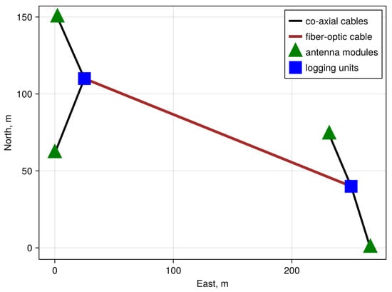
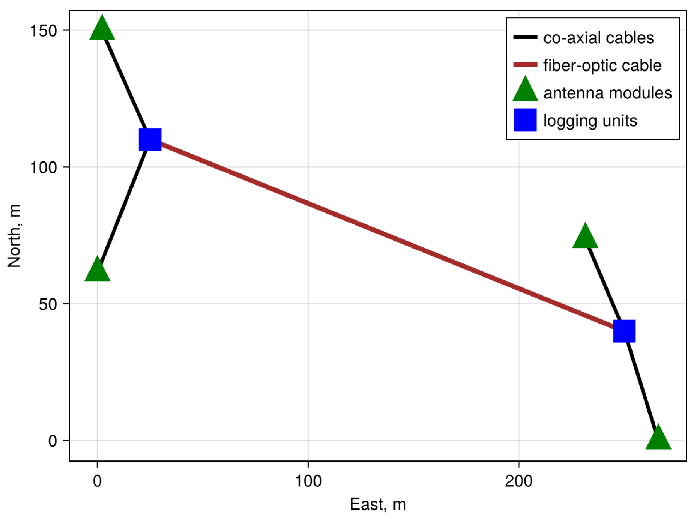
The observations of thundercloud radio emissions are conducted at the receiving point in the Upper Volga region near Nizhny Novgorod with geographic coordinates of 56°9′ N, 44°19′ E. A specially designed system is used for recording the waveform of short electromagnetic pulses operating in the frequency range from 50 kHz to 30 MHz, covering the short-, medium-, and partially long-frequency bands. The installation is a spaced four-point receiving system with a short baseline of approximately 250 m in the east–west direction and approximately 150 m in the orthogonal direction. It is capable of recording up to about two-second individual events (for instance, lightning discharges). Also, it gives an opportunity to determine the direction of arrival of radio emission from sources in these events. Four antenna modules and two four-channel data logging units are used to receive and record radio emissions. The antenna module arrangement is shown in Figure 1.

Figure 1. The antenna module arrangement at the receiving point.

The antenna modules are similar to those described in detail in [7,8]. In brief, each antenna module contains three individual antennas: two mutually perpendicular loop antennas for measuring the horizontal component of the magnetic field and one rod antenna for measuring the vertical component of the electric field. All three antennas are active and contain amplifiers that provide an operating range of 50 kHz to 30 MHz by filtering both low and high frequencies beyond this range. This is needed to reduce the influence of low-frequency interference and to match the output signal to the sampling frequency of the recording devices. Also, the amplifiers serve to match antennas to coaxial cables connecting the antenna modules to the logging units.

Pairs of antenna modules are connected by equal-length cables, each to its own logging unit. The logging units use four-channel 14-bit analog-to-digital converters (ADCs) with a maximum clock rate of 60 MHz and 1 GB internal memory. Antenna module outputs are continuously recorded into a circular buffer organized in the ADC’s internal memory. After a synchronizing (trigger) pulse arrives to the logging unit, recording continues for a preset period of time. After that the entire buffer is copied to RAM and then to the computer’s hard drive, ensuring signal recording both before and after the trigger pulse. The trigger pulse is fed to the second logging unit via a fiber optic cable ensuring that both units record the same event. Using an ADC clock rate of 60 MHz the duration of continuous recording can reach about two seconds, which typically exceeds the duration of a lightning discharge.

Sensitivities of antenna modules (antenna+amplifier) were estimated at several frequencies in the HF range observing known sources of radiation. The estimation was done in the order of value, and 1 V of the ADC output corresponds to a magnetic field strength of 3 · 10⁻³ A/m (approximately corresponds to an electric field strength of 1 V/m).

In monitoring mode the system operates continuously and autonomously. A trigger pulse is generated by a receiver of low-frequency (below 10 kHz) radio emission accompanying a lightning strike. The trigger pulse amplitude threshold is selected based on the requirement for reliable lightning detection and a low probability of triggering from random events unrelated to lightning discharges.

Magnetic antennas are typically used in observations due to the high level of low-frequency interference in the vertical component of the electric field. The recording duration of an individual event in monitoring mode is set to 1.5 s with a prehistory—the recording time before the arrival of the trigger pulse—of 0.5 s.

3. Data Preprocessing

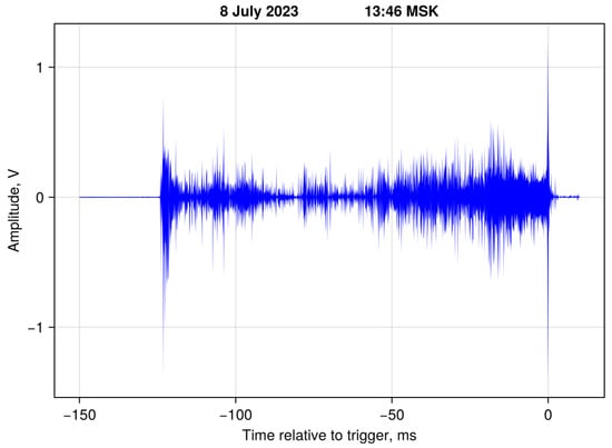
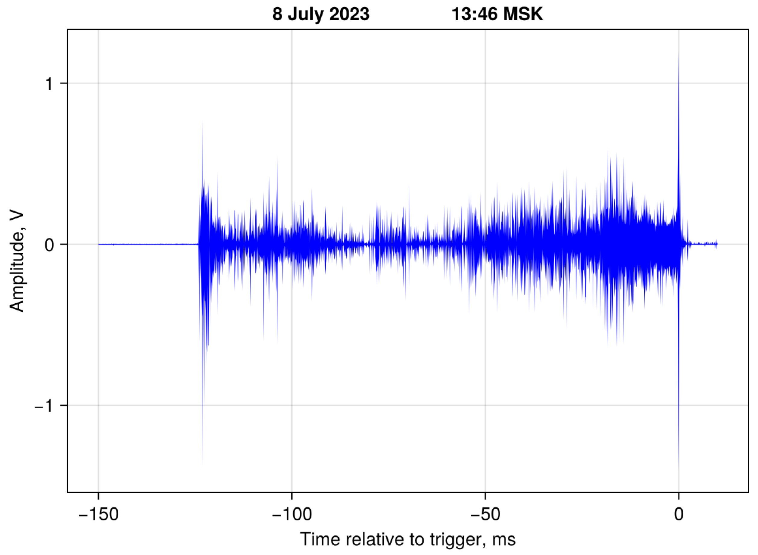
Figure 2 shows an example of radio emission from a cloud-to-ground lightning discharge recorded on 8 July 2023 at 13:46 MSK (UT + 3 h). This lightning is characterized by a relatively long (approximately 100 ms) intracloud development. There is a virtually complete absence of thundercloud emission (at the sensitivity level of the equipment used) more than 300 ms before its onset. It is clear from Figure 2 that the lightning emission amplitude significantly exceeds the background level.

Figure 2. Example of broadband recording of radio emission from a cloud-to-ground lightning discharge; 1 V of the ADC output approximately corresponds to magnetic field strength of $3·{10}^{-3}$ A/m (or electric field strength of ≈1 V/m).

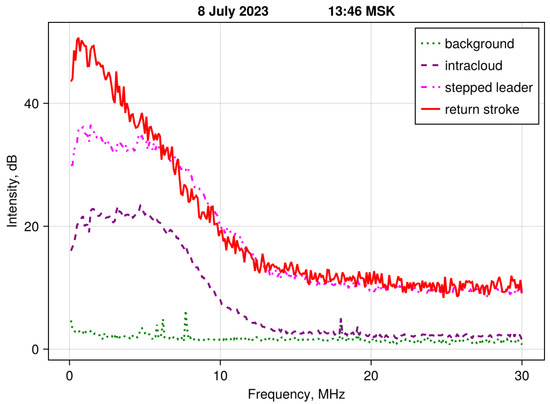
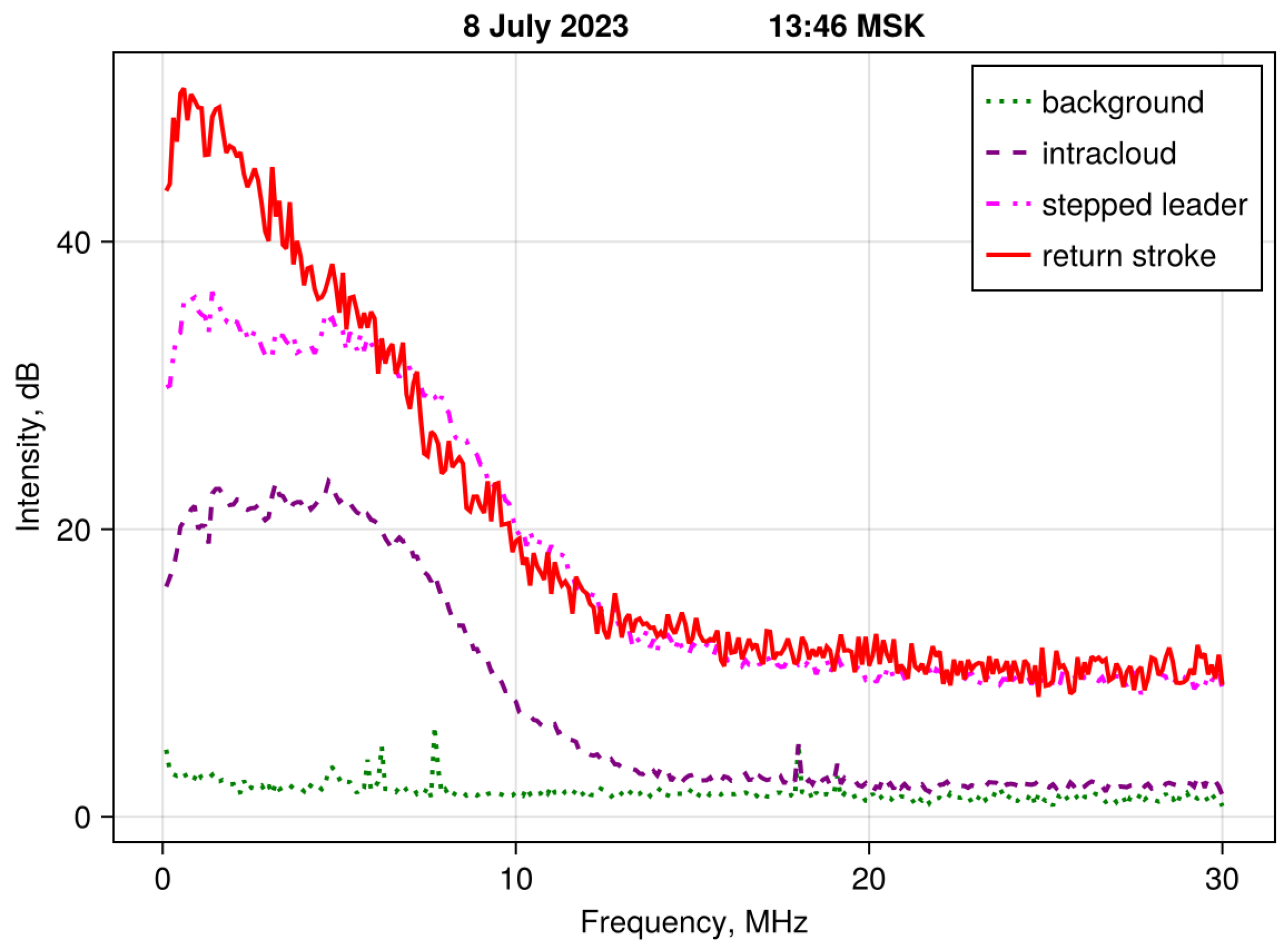
The same is confirmed by the radio emission spectra shown in Figure 3. Spectra were obtained before the onset (background) of the lightning discharge and at various stages of its development: intracloud, stepped leader, and return stroke. The stages of lightning discharge development were determined based on the behavior of the statistical parameters of the lightning emission and the angles of its arrival (see below). At all stages of the discharge’s development the intensity of its radio emission in the frequency range up to 10 MHz exceeds the background intensity significantly. It should be mentioned that averaged spectra of essentially pulsed lightning emission are shown in the Figure 3. The amplitudes of lightning pulses exceed the background level more significantly, up to 60 dB and more. During the intracloud stage of lightning development, the spectrum exhibits a pronounced maximum at frequencies of several MHz, corresponding to the characteristic duration of the emission pulses. However, at this stage the emission intensity does not differ from the background level at frequencies above 15 MHz (for a given receiver sensitivity). The average emission intensity increases during the development of the stepped leader, still maintaining a maximum at frequencies of several MHz. Furthermore, noticeable emission appears at higher frequencies up to the upper limit of the receiving frequency of 30 MHz. The spectrum’s shape changes significantly at the return stroke stage with the expected sharp increase towards low frequencies but coinciding with the spectrum of the stepped leader at frequencies above approximately 6 MHz.

Figure 3. Radio emission spectra in the frequency range 50 kHz–30 MHz before the start of a lightning discharge (background) and at its various stages: intracloud, stepped leader, and return stroke.

Already in the first observations, a predominantly pulsed nature of thundercloud radio emission in the above frequency range was discovered [7,8]. It was found that characteristic pulse lengths are of hundreds of nanoseconds and interpulse intervals are of several to tens of microseconds. In accordance with this, two indicators of the presence of a pulsed component in the received signal were proposed when the interpulse intervals significantly exceed the pulse length [17]. Both indicators are associated with an analysis of the distribution of signal values over specific time intervals that should be selected in accordance with the parameters of the observed pulses, in the range from fractions to units of milliseconds for lightning observations. In the first stage of preliminary data processing, an analysis of the specified distributions is carried out in each of the recording channels in order to verify the observation of a lightning discharge.

The first indicator of the presence of a pulsed component is based on the fact that it increases the root mean square value of the received signal distribution directly related to its intensity while leaving its median absolute deviation virtually unchanged. The ratio of the root mean square value to the median absolute deviation for a pulsed signal in the absence of noise will tend to infinity, for a harmonic signal it is equal to one, and for Gaussian noise it is approximately 1.4826.

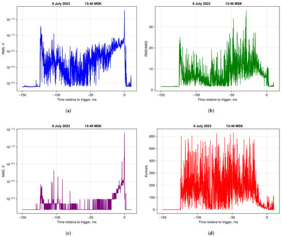
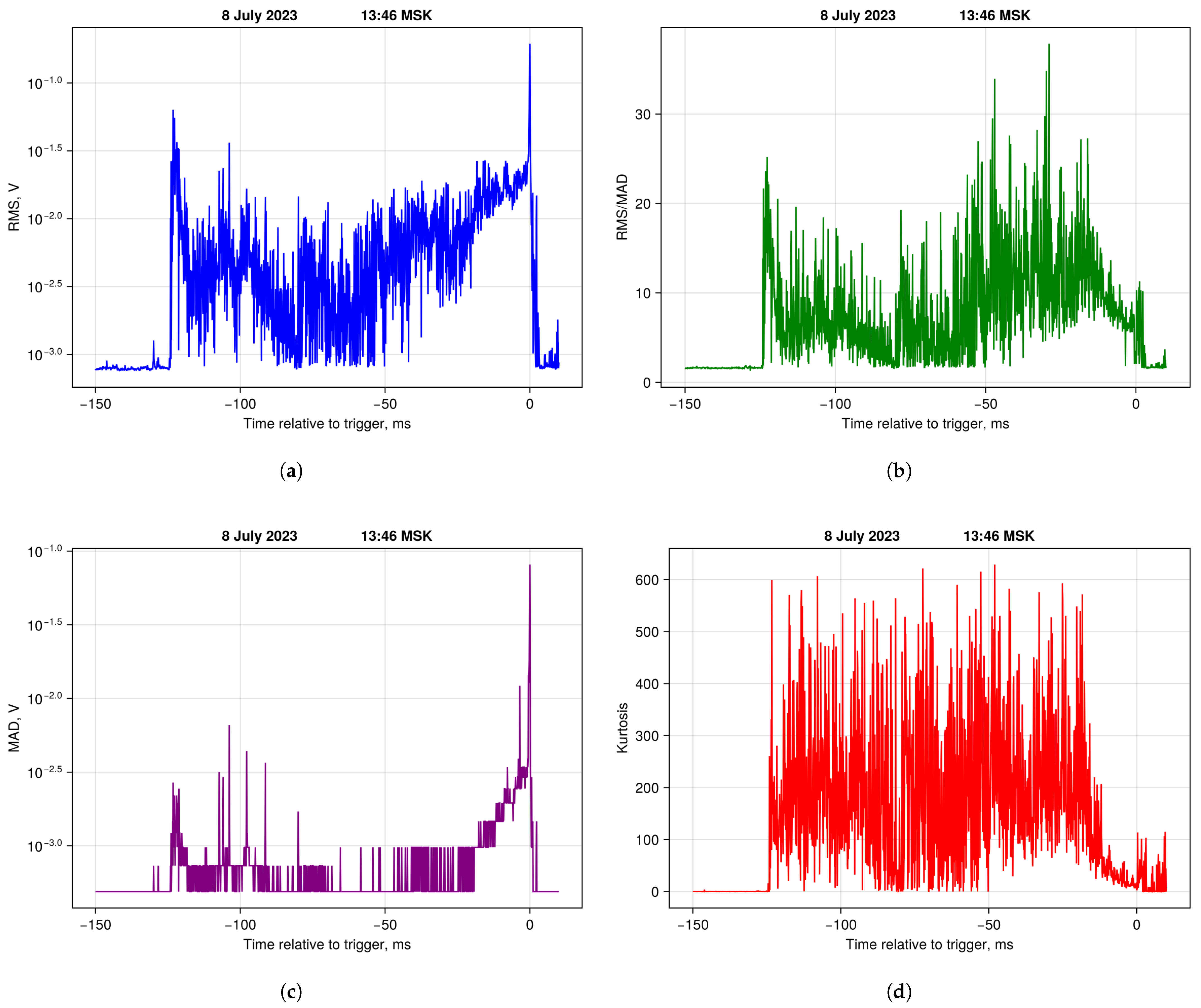
For the event under consideration (see Figure 2), the root mean square value of the received signal amplitude with averaging intervals of 100 μs is shown in Figure 4a. Note its strong fluctuations at the intracloud stage of lightning development (from the onset of the event at approximately 125 ms to approximately 20 ms before the trigger pulse), their significant decrease with relatively small changes in the average level at the stepped leader stage (started approximately 20 ms before the trigger pulse), and a sharp peak during the return stroke (trigger pulse).

Figure 4. (a) RMS values of emission amplitude on intervals of 100 μs. (b) The ratio of the root mean square value of the amplitude to its median absolute deviation. (c) Median absolute deviations of emission amplitude on the same intervals. (d) Kurtosis calculated on the same intervals.

Figure 4c shows the median absolute deviation for the same event and averaging intervals. It is evident from Figure 4c that in the intracloud development stage it has a very small difference from its background level (corresponding to Gaussian noise) indicating the almost pure pulsed nature of the emission at this stage. Median absolute deviation slowly increases during the stepped leader stage, appearing as a quasi-continuous (noise) component in the emission alongside with the pulsed component, and with a sharp peak at the return stroke.

Figure 4b shows the ratio of the root mean square amplitude (RMS, Figure 4a) to the median absolute deviation (MAD, Figure 4c). This ratio is quite high and fluctuates strongly during the intracloud lightning development stage, decreases as the stepped leader develops, and approaches a value corresponding to Gaussian noise at the return stroke.

Another indicator of the presence of pulsed radiation is based on higher-order statistics being more sensitive. This involves analyzing the kurtosis of the distribution of received signal values, which characterizes the sharpness of the distribution function. For a harmonic signal, the kurtosis is −1.5, for Gaussian noise it is zero, and for a pulsed signal it takes on large values determined by the pulse duty cycle.

The kurtosis for the event under consideration for the same averaging intervals of 100 microseconds is shown in Figure 4d. During the intracloud lightning development stage the kurtosis attains very high values, indicating the presence of rare and high-amplitude pulses, and fluctuates significantly. As the stepped leader develops the kurtosis decreases significantly and approaches zero at the return stroke.

This decrease in the kurtosis with the start of stepped leader development toward the ground approximately 20 ms before the return stroke could be used to predict cloud-to-ground lightning discharges. Calculating the kurtosis does not require significant computational effort and can be performed in real time.

Judging by Figure 4b,d, this event actually did record a cloud-to-ground lightning discharge.

The next preprocessing issue is the timing of the data obtained by the two logging units. The ADCs used are not synchronized in their digital clock frequencies. Each has its own clock generator and their frequency can differ from nominal and have a long-term stability of approximately 10⁻⁵. This stability is sufficient for determining both the characteristics of individual pulses and the main stages of lightning discharge development. But it is clearly insufficient for calculating the arrival time delays of pulses recorded by different logging units. With a sampling frequency of 60 MHz and a record length of 1.5 s the clock shift between logging units can reach several microseconds, which is unacceptable for determining delay times. The hardware implementation of synchronization between the logging units presented certain difficulties, and it was decided to transfer this task to the processing layer.

The goal of this data preprocessing stage is to determine the ratio of the digital clock frequencies of the logging units with an accuracy of at least 10⁻⁸. The idea is to use signals from radio stations operating in carrier mode and having sufficient intensity to be extracted directly from the data recorded for each individual event. There are at least a dozen suitable radio stations in the HF band including broadcasting stations.

The clock frequency ratio of logging units can be determined by the ratio of the frequencies of a given radio station recorded by each unit obtained under the assumption of a fixed predetermined sampling rate identical for each unit. Knowledge of the radio station’s frequency in this case is not necessary. The accuracy of frequency determination depends on two factors: the length of the recording from which it is determined and the (spectral) signal-to-noise ratio for a given radio station. Frequency determination accuracy, corresponding to the reciprocal of the recording length, can be significantly improved with a high signal-to-noise ratio.

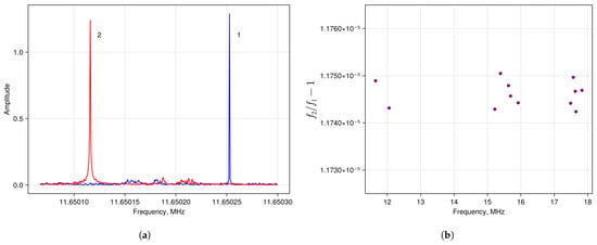
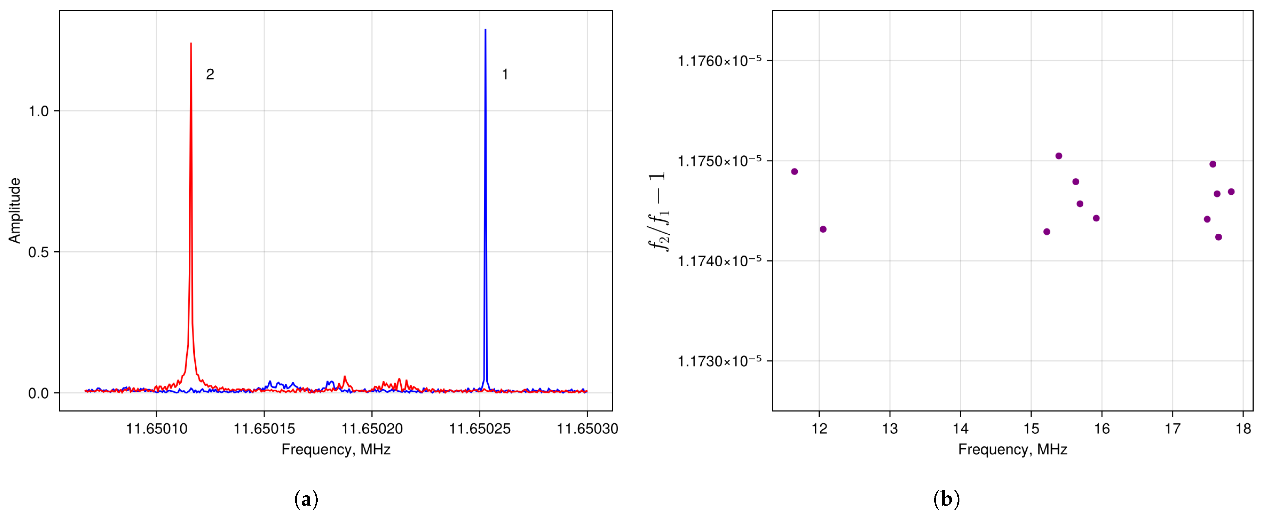
There are a number of methods to determine the frequency of a monochromatic signal with a high signal-to-noise ratio. We applied a method based on the use of three discrete Fourier transform coefficients [18]. Figure 5a shows spectra in the vicinity of 11.65 MHz, obtained at the eastern (1) and western (2) logging units (see Figure 1) under the assumption that the sampling frequency of both units is exactly 60 MHz. The signal-to-noise ratio in this case is quite high and exceeds 40 dB. Figure 5b shows the results of determining the sampling frequency ratio using several broadcast radio stations operating in the 25, 19, and 16 m wavelength bands. Figure 5b demonstrates that this ratio is determined with an accuracy no worse than the required 10⁻⁸.

Figure 5. (a) Emission spectra in the vicinity of a frequency of 11.65 MHz, obtained at the eastern (1) and western (2) logging units under the assumption that the sampling frequency is exactly 60 MHz. (b) Results of determining the ratio of sampling frequencies of logging units. $f_1$ and $f_2$ are sampling frequencies of the eastern and western logging units correspondingly, one is subtracted from the ratio to make the y-axis more readable.

4. Direction of Arrival of Emission Pulses and Lightning Discharge Tracing

The direction to the pulsed radiation source can be determined by the pulse arrival time delay at spatially separated antennas. Assuming the antennas are placed on a horizontal plane according to the plane wave approximation, one can find that the difference in pulse arrival times at a pair of antennas is determined by $\Delta t=-dcos(\Theta )cos(\Phi -\phi )$, where d is the distance between the antennas, $\phi$—azimuth of the direction between the antennas, $\Phi$—source azimuth, and $\Theta$—source elevation angle. Using this relationship for two pairs of non-collinear antennas for the azimuth and elevation angle of the source, one can easily obtain well-known expressions for the direction of pulse arrival as

$$tan(\Phi )={\displaystyle \frac{\Delta t_2{d}_{1}cos\left({\phi }_1\right)-\Delta t_1{d}_{2}cos\left({\phi }_2\right)}{\Delta t_1{d}_{2}sin\left({\phi }_2\right)-\Delta t_2{d}_{1}sin\left({\phi }_1\right)}},cos(\Theta )=-{\displaystyle \frac{\Delta t_1}{d_{1}cos(\Phi -{\phi }_1)}},$$

where the indices correspond to antenna pairs. These ratios can be used for different antenna pairs, which, on the one hand, can reduce the error in determining the angles of arrival of radio pulses, and on the other, can adjust the delay time between logging unit responses.

To solve the problem of tracing lightning discharges, it is first necessary to identify their radio pulses. Since the amplitude of many of these pulses significantly exceeds the background level, only pulses with high amplitudes, exceeding the standard deviation for the background by more than 10 times, were identified. The intervals of possible pulse presence were determined based on the maximum values of the covariance functions of the channels of each logging unit at intervals of 64 ADC samples (approximately one microsecond). The covariance functions were calculated with a shift of eight ADC samples, which ensured that the same pulse fell into several consecutive intervals. Obtained covariance functions were approximated by qubic spline to find a position of its maxima (corresponding to the time delay of signal arrival between the antenna modules) with an accuracy of 0.1 of the sampling period. A pulse was considered to correspond to a certain emission source if these maxima differed by no more than 0.1 of the sampling period for several (usually five) consecutive intervals. Based on the time delays determined in this way, the arrival angles (azimuth and zenith angle) of the radio emission pulse were calculated.

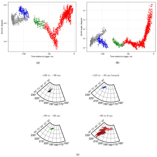
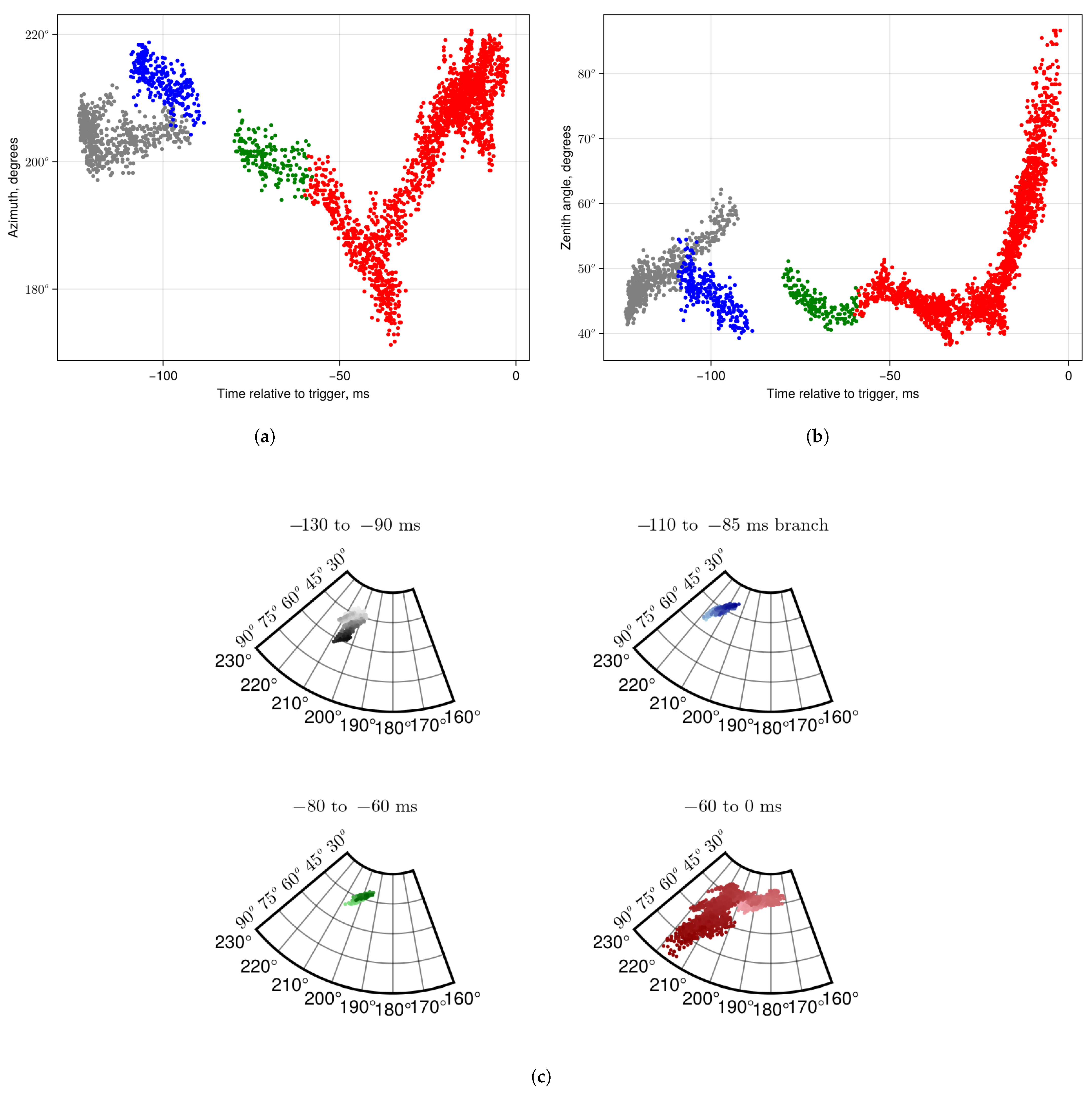
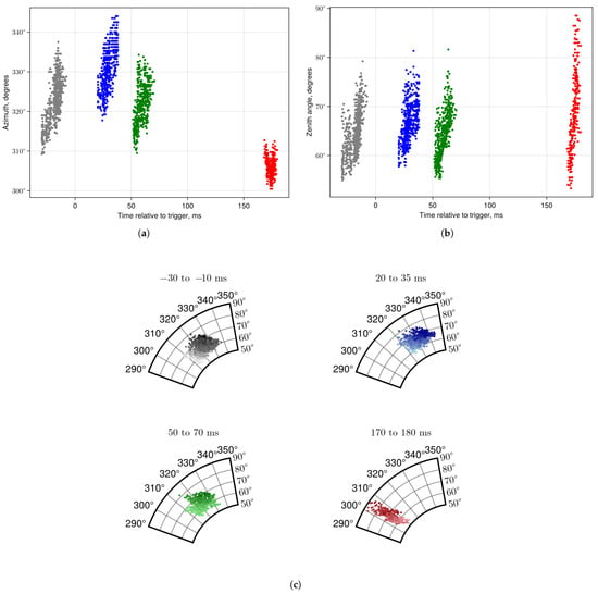
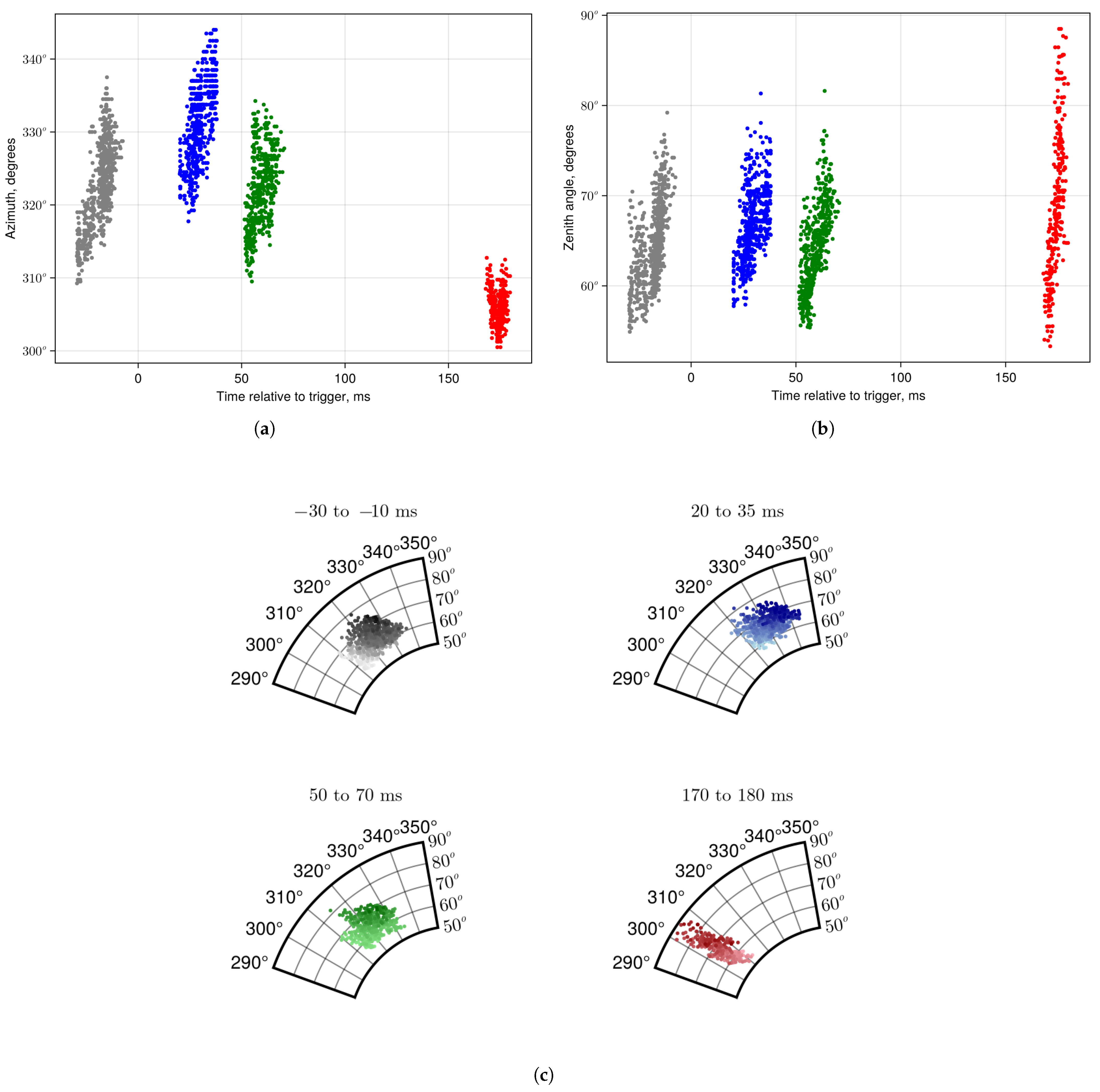
Since individual pulses in a thundercloud generally can be emitted from unconnected points, lightning discharge traces were identified as trains of pulses based on the principle of a small distance between them in time and in delays between antennas. The DBSCAN (Density-Based Spatial Clustering of Applications with Noise) algorithm is used for this purpose. For the event under consideration, trains of at least 50 pulses were selected, for which the distance between adjacent pulses did not exceed 0.2 of a sampling period in delay and 1 millisecond in time. Four such (irregular) trains were found and are presented in Figure 6. The upper panels of Figure 6 show the temporal development of azimuth (left, Figure 6a) and zenith angle (right, Figure 6b) for all pulse trains. The lower panel (Figure 6c) shows pulse trains individually in the azimuth–zenith angle polar coordinates; the brightness of the color corresponds to the time, with darker colors corresponding to later times.

Figure 6. Pulse trains of the event recorded on 8 July 2023 at 13:46 MSK. Colors correspond to different trains: first train is shown in gray, second—in blue, third—in green, fourth—in red. (a) Temporal development of pulse train azimuth. (b) Temporal development of pulse train zenith angle. (c) Polar plots of each pulse train in the azimuth–zenith angle plain. Approximate time to trigger intervals are given above each plot. Colors correspond to ones in the upper panels (a,b). The brightness of the color corresponds to the time, with darker colors corresponding to later times.

The first pulse train consisted of 589 pulses which began ∼125 ms before the trigger at a zenith angle of ∼40° (elevation angle of ∼50°) and an azimuth of ∼210°. This is shown in the upper left panel of Figure 6c. This train lasted until ∼90 ms before the trigger with a permanently increasing zenith angle and a variable azimuth. It seems that this train likely corresponds to an incomplete lightning discharge directed toward the ground which, however, did not reach its surface.

The second train consisted of 275 pulses, which began later at ∼110 ms before the trigger at a zenith angle close to the zenith angle of the first train at that time but differed by about 10° azimuth. This is shown in the upper right panel of Figure 6c. This train definitely corresponds to an intracloud discharge directed to the receiving point due to a permanently decreasing zenith, and was ended approximately at the same time as the first train.

There is a gap of about 10 ms after the ending of the first two trains when no trains with the given characteristics were found. This could be seen as a confirmation that the first train is really a discharge towards the ground.

The third train consisted of 175 pulses, which began at ∼80 ms before the trigger at a zenith angle of ∼50° and an azimuth of ∼200°. This is shown in the lower left panel of Figure 6c. As the second example of this, this train definitely corresponds to an intracloud discharge directed to the receiving point and ended at ∼60 ms before the trigger.

The fourth train is the largest one and consisted of 2033 pulses. It is shown in the lower right panel of Figure 6c. This train likely continued the third one and ended at a trigger time with zenith angles close to ground. At about 40 ms before the trigger, it exhibited azimuthal branching with one branch developed to the east at an azimuth of ∼170° at an approximately constant zenith angle of ∼45°, and another developed to the ground corresponding to a lightning strike at an azimuth of ∼215°. It should be noted that the poor resolution of the array for the zenith angle near the horizon may be responsible for the strong blurring of this train at large zenith angles.

In total, the intracloud discharge stage developed at zenith angles of 40° to 50° excluding an incomplete discharge to the ground approximately 90 ms before the trigger. The lightning initiation processes occurred at an azimuth of ∼200°. Subsequently, branching was observed as the discharge developed, and the azimuth of the direction to the emission sources changed significantly. A continuous increase in the zenith angle was observed during the stepped leader stage corresponding to discharge approach to the ground. A broadening of the emission source region in both azimuth and zenith angle was observed near the return stroke which was apparently related to a decrease in the accuracy of zenith angle determination near the horizon.

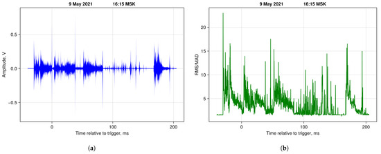
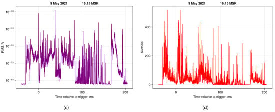
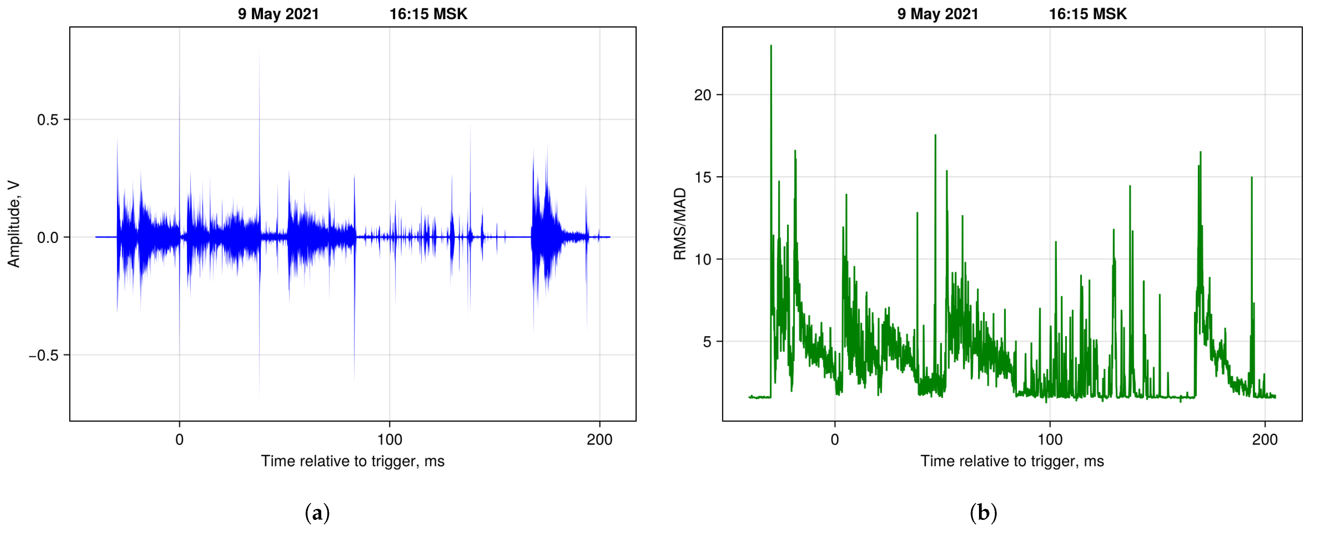
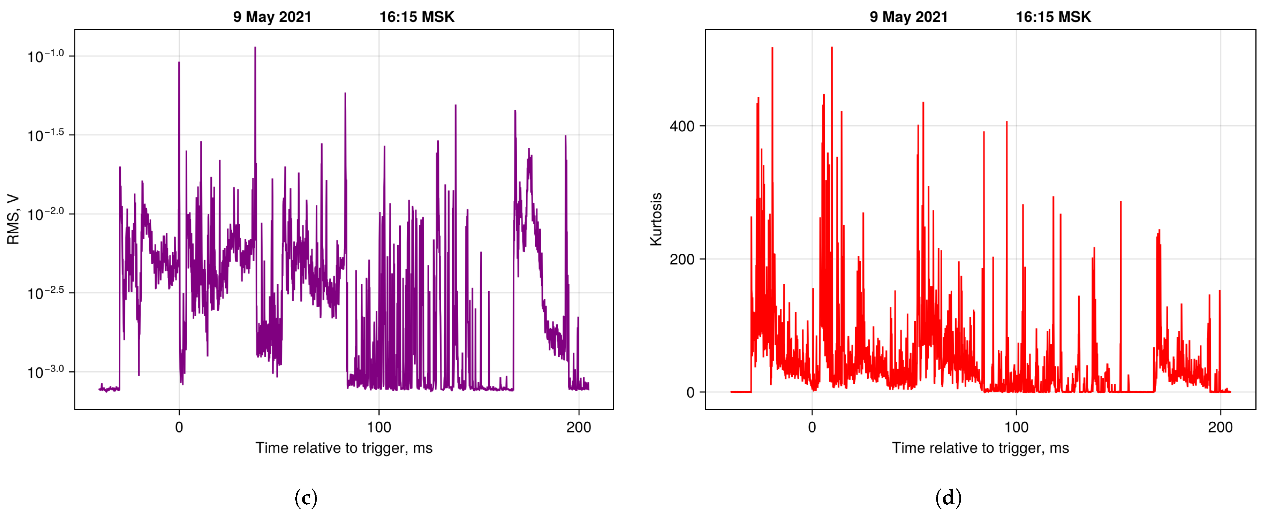
Another example of radio emission from multiple cloud-to-ground lightning discharges recorded on 9 May 2021 at 16:15 MSK is shown in Figure 7 and Figure 8.

Figure 7. Radio emission from thundercloud recorded on 8 July 2023 at 13:46 MSK. (a) Amplitude of radio emission. (b) The ratio of the RMS value of the amplitude to its median absolute deviation on the same intervals. (c) RMS value of emission amplitude on intervals of 100 microseconds. (d) Kurtosis on the same intervals.

Figure 8. Pulse trains of the event recorded on 9 May 2021 at 16:15 MSK. Colors correspond to different trains: first train is shown in gray, second—in blue, third—in green, fourth—in red. As in Figure 6: (a) Temporal development of pulse train azimuth. (b) Temporal development of pulse train zenith angle. (c) Polar plots of each pulse train in the azimuth–zenith angle plain. Approximate time to trigger intervals are given above each plot. Colors correspond to ones in the upper panels (a,b). The brightness of the color corresponds to the time: darker colors—later time.

In Figure 7 the amplitude of a recorded signal along with its root mean square, root mean square to median absolute deviation, and kurtosis are shown. At least three strikes to the ground can be seen from the emission behavior.

For this event, trains of at least 100 pulses were selected with the same constraints on the distance between adjacent pulses (that they should not exceed 0.2 of a sampling period in delay and 1 ms in time). Four trains were found and are presented in Figure 8. As in Figure 6, the upper panels of Figure 8 show the temporal development of azimuth (left, Figure 8a) and zenith angle (right, Figure 8b) for all pulse trains. The lower panel (Figure 8c) shows pulse trains individually in the azimuth–zenith angle polar coordinates; the brightness of the color corresponds to the time, with darker colors corresponding to later times.

All the trains consisted of 700, 565, 466, and 294 pulses, which correspond to different cloud-to-ground lightning discharges that originated at a ∼55° zenith angle but different azimuths.

5. Discussion and Conclusions

Observations carried out in the Upper Volga region demonstrated the feasibility of using the HF band for observations of lightning discharge radio emission. At all stages of lightning development the intensity of its radio emission in the frequency range up to 10 MHz exceeded the average background intensity significantly. The amplitudes of lightning pulses exceeded the background level more significantly, up to 60 dB and more.

The pulsed nature of the lightning emission in the above frequency band makes it possible to determine the direction of arrival of individual pulses and trace sources of lightning emission. Single-point observations only allow for the two-dimensional mapping of lightning discharges by azimuth and zenith angle. Additional points spaced 10–20 km apart could enable three-dimensional mapping and, in particular, the location of lightning strikes to the ground.

From this point of view observations in the HF band could compete with the widely used VHF band. An advantage of HF band use is the higher intensity of lightning emission in this band compared with VHF and therefore less stringent requirements for receiving equipment. Interference in the HF band is insignificant for observations of lightning discharges due to the high intensity of emission of the latter.

Moreover, the possibility of the ultra-short-term (about 20 ms) prediction of nearby lightning strikes could be proposed based on monitoring the behavior of the kurtosis of the thundercloud emission amplitude distribution over short (about 100 ms) timescales. Note that calculating the kurtosis does not require significant computational effort and can be performed in real time.

References

- World Wide Lightning Location Network—WWLLN. Available online: http://wwlln.net/ (accessed on 21 December 2025).
- Koshak, W.J.; Krider, E.P.; Murray, N.; Boccippio, D.J. Lightning charge retrievals: Dimensional reduction, LDAR constraints, and a first comparison with LIS satellite data. J. Atmos. Ocean. Technol. 2007, 24, 1817–1838. [Google Scholar] [CrossRef] [Scilit]
- Edens, H.E.; Eack, K.B.; Eastvedt, E.M.; Trueblood, J.J.; Winn, W.P.; Krehbiel, P.R.; Aulich, G.D.; Hunyady, S.J.; Murray, W.C.; Rison, W.; et al. VHF lightning mapping observations of a triggered lightning flash. Geophys. Res. Lett. 2012, 39, L19807. [Google Scholar] [CrossRef] [Scilit]
- van der Velde, O.A.; Montanyà, J.; Soula, S.; Pineda, N.; Mlynarczyk, J. Bidirectional leader development in sprite-producing positive cloud-to-ground flashes: Origins and characteristics of positive and negative leaders. J. Geophys. Res. Atmos. 2014, 119, 12755–12779. [Google Scholar] [CrossRef] [Scilit]
- Chronis, T.; Lang, T.; Koshak, W.; Blakeslee, R.; Christian, H.; McCaul, E.; Bailey, J. Diurnal characteristics of lightning flashes detected over the São Paulo lightning mapping array. J. Geophys. Res. Atmos. 2015, 120, 11799–11808. [Google Scholar] [CrossRef] [Scilit]
- Caicedo, J.A.; Uman, M.A.; Pilkey, J.T. Lightning evolution in two north-central Florida summer multi-cell storms and three winter/spring frontal storms. J. Geophys. Res. Atmos. 2018, 123, 1155–1178. [Google Scholar] [CrossRef] [Scilit]
- Gurevich, A.V.; Duncan, L.M.; Karashtin, A.N.; Zybin, K.P. Radio emission of lightning initiation. Phys. Lett. A 2003, 312, 228–237. [Google Scholar] [CrossRef] [Scilit]
- Karashtin, A.N.; Shlyugaev, Y.V.; Gurevich, A.V. High-frequency radio emission of the lightning discharge. Radiophys. Quantum Electron. 2005, 48, 711–719. [Google Scholar] [CrossRef] [Scilit]
- Gurevich, A.V.; Karashtin, A.N. Radio emission structure of cloud-to-ground lightning discharge. Phys. Lett. A 2011, 375, 1128–1134. [Google Scholar] [CrossRef] [Scilit]
- Nag, A.; Rakov, V.A. Electric field pulse trains occurring prior to the first stroke in negative cloud-to-ground lightning. IEEE Trans. Electromagn. Compat. 2009, 51, 147–150. [Google Scholar] [CrossRef]
- Nag, A.; DeCarlo, B.A.; Rakov, V.A. Analysis of microsecond- and submicrosecond-scale electric field pulses produced by cloud and ground lightning discharges. Atmos. Res. 2009, 91, 316–325. [Google Scholar] [CrossRef] [Scilit]
- Lan, Y.; Zhang, Y.; Dong, W.; Lu, W.; Liu, H.; Zheng, D. Broadband analysis of chaotic pulse trains generated by negative cloud-to-ground lightning discharge. J. Geophys. Res. 2011, 116, D17109. [Google Scholar] [CrossRef] [Scilit]
- Zhang, Y.; Zhang, Y.; Li, C.; Lu, W.; Zheng, D. Simultaneous optical and electrical observations of “chaotic” leaders preceding subsequent return strokes. Atmos. Res. 2016, 170, 131–139. [Google Scholar] [CrossRef] [Scilit]
- Hare, B.M.; Scholten, O.; Bonardi, A.; Buitink, S.; Corstanje, A.; Ebert, U.; Falcke, H.; Hörandel, J.; Leijnse, H.; Mitra, P.; et al. LOFAR lightning imaging: Mapping lightning with nanosecond precision. J. Geophys. Res. Atmos. 2018, 123, 2861–2876. [Google Scholar] [CrossRef] [Scilit] [PubMed]
- Scholten, O.; Hare, B.M.; Dwyer, J.; Sterpka, C.; Kolmašová, I.; Santolík, O.; Lán, R.; Uhlíř, L.; Buitink, S.; Corstanje, A.; et al. The initial stage of cloud lightning imaged in high-resolution. J. Geophys. Res. Atmos. 2021, 126, e2020JD033126. [Google Scholar] [CrossRef] [Scilit]
- Scholten, O.; Hare, B.M.; Dwyer, J.; Liu, N.; Sterpka, C.; Assink, J.; Leijnse, H.; Veen, S.t. Small-scale discharges observed near the top of a thunderstorm. Geophys. Res. Lett. 2023, 50, e2022GL101304. [Google Scholar] [CrossRef] [Scilit]
- Karashtin, A.N.; Shlyugaev, Y.V.; Karashtina, O.S. Cloud-to-ground lightning discharge indicator in the radio frequency emission of thunderclouds as observed in the Upper Volga region of Russia. Atmos. Res. 2021, 256, 105559. [Google Scholar] [CrossRef] [Scilit]
- Candan, C. A method for fine resolution frequency estimation from three DFT samples. IEEE Signal Process. Lett. 2011, 18, 351–354. [Google Scholar] [CrossRef] [Scilit]
Disclaimer/Publisher’s Note: The statements, opinions and data contained in all publications are solely those of the individual author(s) and contributor(s) and not of MDPI and/or the editor(s). MDPI and/or the editor(s) disclaim responsibility for any injury to people or property resulting from any ideas, methods, instructions or products referred to in the content. |
© 2026 by the authors. Licensee MDPI, Basel, Switzerland. This article is an open access article distributed under the terms and conditions of the Creative Commons Attribution (CC BY) license.