


Abstract
This study develops a practical framework for forecasting long-term drought conditions in Karaman Province, a semi-arid region of Turkey, where accurate climate information is vital for water planning and agriculture. Since the area has limited rainfall records and strong year-to-year fluctuations, traditional modeling approaches often fall short. To better capture local conditions, drought intensity was defined using a simple monthly wetness anomaly measure based directly on precipitation; here, positive values indicate wetter months and negative values indicate drier ones. This makes the method suitable for regions where detailed hydrological data are scarce. Rainfall observations from 1965 to 2011 were expanded using a combination of kernel density estimation and Cholesky-based correlation reconstruction. These steps preserved the main statistical and temporal patterns of the original data while increasing sample diversity. The enriched dataset was then used to train artificial neural networks to predict both precipitation and drought intensity. The models reached R2 values of 0.76 and 0.72, with mean absolute errors of 12.8 mm and 28.4%, which represents an improvement of roughly 10–15% over traditional statistical methods. They were also able to capture the seasonal and year-to-year variability that strongly affects drought conditions in the region. To understand what drives the predictions, the model was examined with LIME, which consistently highlighted lagged rainfall and seasonal indicators as the most influential inputs. A walk-forward validation approach was also used to mimic real forecasting conditions and demonstrated that the model remains stable when projecting into the future. Overall, the proposed framework offers a reliable and practical basis for early-warning efforts and drought-management strategies in semi-arid regions like Karaman.
1. Introduction
Drought is increasingly regarded as one of the most difficult natural hazards to characterize because it emerges slowly and does not show clear early warning signs. Unlike sudden natural events, its development may extend over many months or even several years, which often prevents timely detection until critical conditions have already been exceeded and recovery becomes extremely challenging. In practical terms, drought acts as a widespread stress factor that affects agricultural production, water distribution systems, and the overall stability of social and economic structures [1,2]. These effects are especially severe in regions where water resources are already limited. Although the literature suggests that long lasting drought might contribute to social tension, the extent of this influence is strongly shaped by local political arrangements and the economic capacity of the affected communities.
In recent years, many studies have begun to interpret drought not as an isolated climatic irregularity but as a reflection of large-scale climate variability that is being intensified by human driven environmental change. Increasing global temperatures are altering atmospheric circulation as well as regional rainfall distributions, which makes continuous drought monitoring even more essential [3,4]. As a result, both the occurrence and severity of drought events are expected to rise in the coming decades. Current scientific assessments indicate that regions with semi-arid and Mediterranean climates will experience the greatest pressure under high emission conditions, and notable changes in aridity indicators are already being projected [5,6]. This shift introduces considerable difficulty for hydrological modeling because most traditional approaches rely on the assumption that the climate system remains stable over time. Such an assumption becomes unreliable when climatic behavior is undergoing rapid transformation [7].
One of the main difficulties in forecasting drought is the limited amount of reliable training data. Many regions still lack consistent observations, and even places with better monitoring often face problems such as missing satellite measurements or areas that are not fully covered [8]. Because of these gaps, researchers have turned to Synthetic Data Generation as a practical way to improve datasets. Approaches like Generative Adversarial Networks, Variational Autoencoders, and copula-based sampling help create new data that follow the same general behavior as real environmental records without changing the long-term climate trends [9,10]. Recent developments in generative artificial intelligence also suggest that these synthetic samples can reproduce rare extreme conditions, which is important for studying long lasting drought events [11]. Another useful approach is time sliding augmentation, which can enlarge small datasets and provide better support for models that rely heavily on data driven learning [9].
Artificial Neural Networks (ANNs), computer frameworks modeled after biological neurons, are extensively employed to identify nonlinear interactions in hydrometeorological systems. ANNs acquire input–output relationships via linked layers of weighted nodes, allowing them to express intricate temporal patterns that conventional statistical models frequently overlook. ANN and Deep Learning (DL) models have shown strong potential for representing the complex and nonlinear behavior of hydrometeorological systems. Recent work suggests that when synthetic data are combined with models such as Convolutional Neural Networks and Recurrent Neural Networks, the accuracy of drought and rainfall predictions improves, especially in places where observations are limited [12,13]. This strategy is also useful for datasets in which extreme conditions appear only a few times and are therefore difficult for models to learn [14,15]. Another direction in current research is the idea of differentiable hydrology, which brings deep learning models together with basic physical rules in order to strengthen their ability to generalize [16]. Data augmentation has also been reported to support both long-term forecasting and short-term rainfall prediction, helping reduce the gap between what is observed and what must be predicted [17].
Turkey provides an important setting for evaluating these methods because it has a semi-arid climate and has experienced many serious droughts. Major drought episodes during the past century have affected both agricultural production and the national water supply system in noticeable ways [18]. The large differences in rainfall from place to place and from year to year within the country also show how important it is to develop reliable modeling tools that can help reduce future risks [19]. In many parts of Turkey, farming practices are especially vulnerable to changes in climate. Recent studies show that approaches based on counterfactual scenarios and data augmentation can support the prediction of crop development and wheat yields under uncertain climate conditions, which is vital for food security in regions that are already at risk [20,21]. This is even more relevant for the Mediterranean basin, which is widely recognized as one of the areas most affected by climate change [22].
Although achieving high accuracy is important, many advanced machine learning models are difficult to use in practice because their internal workings are not easy to understand. For this reason, Explainable Artificial Intelligence tools have become increasingly important. Methods that clarify how a model reaches its decisions help improve transparency and build confidence among practitioners and policy makers [23,24]. Neural network designs that include physical reasoning are especially valuable for studying earth system processes. They help ensure that the predictions follow basic physical and hydrological principles rather than simply reflecting patterns in the data that may not be meaningful [25,26].
Central Anatolia has a cold semi-arid continental climate, marked by scorching, arid summers and frigid winters with significant snowfall. Winter precipitation manifests as both rain and snow, with snowfall generally accounting for 30–50% of total winter precipitation in urban basins like Karaman. Snow cover often endures for 2–6 weeks, contingent upon altitude, and shallow soil freezing is sometimes noted from December to February, attributed to average winter temperatures ranging from 0 to 3 °C. The winter conditions are vital for hydrology, since snow accumulation and subsequent spring thaw enhance soil moisture recharge and postpone infiltration processes across Central Anatolia [27].
This research looks at long-term drought prediction in Karaman Province, Turkey, drawing on monthly precipitation data from 1965 to 2011. To strengthen the dataset—and give models more to work with synthetic data augmentation is applied. It is a way of filling in gaps, in a sense, while preserving the underlying trends. The enriched dataset is then used to train ANNs, which are known to handle nonlinear and sequential patterns well. In parts of Central Anatolia, water scarcity is not just a seasonal concern; it is increasingly persistent. The ability to forecast drought with reasonable lead time can make a difference, not just for crop planning, but also for how regional water and economic systems hold together during extended dry periods. Despite recent advancements in machine learning based drought forecasting, existing models often rely on limited observational datasets and lack temporal generalization capacity. Most hybrid approaches either focus on short-term forecasting or ignore the scarcity of long-term, high-resolution data in semi-arid regions. This study addresses this gap by integrating synthetic data augmentation with interpretable neural models to improve long-term drought prediction in data-scarce Mediterranean ecosystems. In summary, this study makes three novel contributions to the field of drought forecasting: (1) it demonstrates the utility of synthetic augmentation in enhancing model robustness under data scarcity; (2) it validates the importance of interpretable machine learning (LIME) in operational settings; and (3) it presents a scalable, regionally adaptable framework that bridges methodological sophistication with practical usability. These aspects collectively push the boundaries of existing machine learning-based drought prediction efforts in semi-arid climates.
2. Materials and Methods
This research utilizes a historical time series dataset from the Karaman area, covering the period from January 1965 to December 2011. The collection initially comprised monthly records for two principal variables: precipitation (mm), quantified millimeters, and drought intensity, articulated as a percentage. Following a comprehensive cleaning and preparation phase eliminating gaps, verifying abnormalities, and synchronizing time steps the final dataset comprised 564 acceptable monthly entries. The result was a continuous time series that, mostly, remained cohesive for model construction and analysis. The consistency was particularly significant, considering the study’s emphasis on long-term drought patterns. This study utilized monthly precipitation data sourced from the Turkish State Meteorological Service (MGM), specifically the long-term observational records from the Karaman meteorological station covering the years 1965 to 2011. All drought intensity figures were obtained from the raw precipitation readings.
The monthly precipitation (P) data was obtained from the General Directorate of Meteorology of Türkiye (MGM), the governmental authority responsible for managing terrestrial meteorological observation networks. The data is obtained from the Karaman provincial meteorological station, which provides continuous, quality-assured precipitation readings recorded in millimeters (mm). The information included in this study encompasses the period from 1965 to 2011 and was obtained via MGM’s official data request and verification mechanism.
Data preprocessing followed a series of standard but essential procedures. Missing and invalid entries were excluded from the dataset, while categorical variables were translated into numerical equivalents suitable for model input. To enable consistent chronological tracking, a time index was created by merging the year and month fields into a single continuous metric. The descriptive statistics indicated significant variability in both principal variables. Monthly precipitation varied from 0 mm to 144 mm, with an average of 27.75 mm and a standard deviation of 24.57 mm. The intensity levels of drought varied from 0% to 514.64%, with a mean of 98.91% and a standard deviation of 87.79%. These values are not unexpected for a semi-arid region, where interannual variability can be substantial. Upon inspection, seasonal patterns became evident in the time series plots. Higher precipitation levels were concentrated in the winter months, while drought intensity tended to rise during drier periods, a pattern that aligns with typical regional climate behavior [28].
A variety of feature engineering strategies were employed to improve model learning and forecast performance. Temporal data that includes the month variable was represented by sine and cosine functions to represent its cyclical characteristics, a prevalent method in seasonal and time-series analysis [29]. In order to capture short-term dependencies, lag features were introduced for both precipitation and drought intensity, covering one-, two-, and three-month intervals. Rolling statistics were also included, calculated over three- and six-month windows, to account for mid-range climatic patterns. In total, this process produced 14 input variables per time step. These features were used to train the predictive models, with the aim of improving their sensitivity to both immediate and evolving temporal dynamics.
To overcome the limited sample size and improve model generalization, data augmentation was performed using Kernel Density Estimation (KDE). This technique involved estimating the probability density function of the observed data in order to generate additional synthetic samples. Based on this estimation, new values were drawn that maintained the statistical properties of the original dataset [30]. As a result, the augmented data retained distributional consistency while increasing the diversity of training inputs. The correlation structure between features was retained using Cholesky decomposition of the empirical correlation matrix, and minor Gaussian noise was added to each synthetic sample to prevent duplication. This approach produced 300 synthetic samples for each target variable, significantly augmenting the training dataset. Statistical validation of the supplemented data’s integrity was conducted using the Kolmogorov–Smirnov (K–S) test. The results indicated no significant variations between the empirical distributions of the original and synthetic datasets at the 5% significance level, affirming that the augmentation maintained the fundamental statistical properties of the observed data [31]. The dataset was initially divided into training and testing subsets employing a temporally consistent methodology. Synthetic data production was conducted solely on the training set, while the test set was maintained as an independent benchmark to avert data leaking.
The KDE/Cholesky method was limited to replicating the observed marginal distributions and covariance structure, guaranteeing that synthetic extremes were physically compatible with the regional hydroclimatic attributes.
For benchmarking, the predictive efficacy of the proposed ANN and LSTM models was juxtaposed with two conventional baseline techniques, henceforth termed ‘traditional methods’. The initial baseline is a Multiple Linear Regression (MLR) model, a commonly employed statistical method that presumes linear correlations between precipitation-related covariates and drought severity. The second baseline is an AutoRegressive Integrated Moving Average (ARIMA) model, utilized to describe linear temporal relationships frequently applied in hydroclimatic time-series forecasting. Both baseline models were trained and assessed utilizing identical data partitions and evaluation measures as the proposed models, hence guaranteeing a consistent and reproducible comparison.
Two Artificial Neural Networks were constructed: one aimed at forecasting precipitation (mm), the other focused on drought intensity. The setup was similar in both cases, though each model was trained separately on its respective target to avoid interference between the learning processes. The architecture started with an input layer of 14 neurons, reflecting the set of engineered features derived during preprocessing. Subsequently, three hidden layers were used, containing 64, 32, and 16 neurons. Each of these applied the ReLU activation function, which has become standard for handling nonlinearity in similar tasks. To help reduce overfitting, dropout regularization was included after the first two hidden layers, with a rate of 0.2. The final layer consisted of a single neuron with a linear activation function, allowing the models to output continuous values. In combination, each network had 3585 trainable parameters [32].
The prediction equations derived from these models can be expressed as follows:
The formula for precipitation (mm) prediction:
The formula for drought intensity prediction:
where is the predicted precipitation (mm) at time t, is the predicted drought intensity (%) at time t, and are the optimized model weights for precipitation and drought models, and are the bias terms for precipitation and drought models, f and g represents the complex non-linear functions implemented by the neural networks, respectively.
represents the input features as follows: x1 = year; x2 = month; x3 = sin(2πx2/12); x4 = cos(2πx2/12); x5 = (precipitation from the previous month); x6 = (precipitation from two months ago); x7 = (precipitation from three months ago); x8 = (drought intensity from the previous month); x9 = (drought intensity from two months ago); x10 = (drought intensity from three months ago); x11 = (three-month rolling mean of precipitation); x12 = (six-month rolling mean of precipitation); x13 = (three-month rolling mean of drought intensity); x14 = (six-month rolling mean of drought intensity).
The neural network design executes these equations via a succession of hidden layers with non-linear activation functions. The Rectified Linear Unit (ReLU) activation function, expressed as ReLU(x) = max(0, x), serves to add nonlinearity into the network and enhance convergence stability by allowing positive signals to transmit while attenuating negative values. The proposed models include three hidden layers using ReLU activations and a linear output layer. h1, h2, and h3 can be calculated as follows: h1 = ; h2 = ReLU(W2 Dropout (h1, 0.2) + b2); h3 = ReLU(W3 Dropout (h2, 0.2) + b3); y = W4 h3 + b4.
Where X is the input feature vector (; are weight matrices for each layer; are bias vectors for each layer; ReLU (x) = max (0,x) is the activation function; randomly sets 20% of the elements to zero during training.
For practical applications, a simplified linear regression approximation of the relationships in the data can be expressed as:
Precipitation (mm) and drought intensity were calculated using the succeeding equations:
where CP and CD are constants derived from the model.
To address the inherent “black box” nature of artificial neural networks and enhance model interpretability, Local Interpretable Model-agnostic Explanations (LIME) analysis was also applied [19,20]. Understanding how complex models arrive at their predictions is critical, especially in areas like drought forecasting, where decisions carry real-world consequences. LIME addresses this need by building simple, local models that mimic the behavior of neural networks around specific outputs. What makes this approach so helpful is its ability to make individual predictions easier to explain. For water managers and policy planners, that clarity matters. It builds trust in model-based tools and helps ensure that forecasts are not only accurate but also usable in planning and mitigation strategies. The LIME analysis was performed on five typical test examples chosen from various time periods and drought conditions to provide thorough coverage of model behavior. And LIME produced explanations for each selected instance by altering the input characteristics and analyzing the resultant variations in model predictions. The perturbation technique entailed generating 1000 synthetic samples for each instance by introducing controlled noise to the feature values while preserving realistic ranges according to the original data distribution. Furthermore, the utilized explainer was configured by treating 14 features as continuous variables. Feature significance scores were derived by fitting linear regression models to the altered samples and their respective predictions. The positive and resultant coefficients represent the features that increased and decreased the predicted values, respectively. A consistency check was also conducted over all revealed occurrences. Features with consistency scores over 80% were considered to have steady and reliable impact patterns, signifying that the model has acquired generalizable connections rather than instance-specific artifacts. The LIME analytical framework can be expressed mathematically as follows:
where stands for the local explanations for instance x, f is the original complex model (ANN), g is the interpretable model (linear regression), G is the class of interpretable models, is the proximity measure defining the neighborhood around x, is the local aware loss function, and is the complexity penalty for the interpretable model. For each explained instance i and feature j, the LIME importance score was calculated as:
where is the coefficient of feature j in the local linear model, is the value of feature j for instance i, is the mean value of feature j in the perturbed neighborhood. And the consistency score for feature j across all explained instances was computed as:
where is the proportion of instances where feature j has a positive influence, and is the proportion where it has a negative influence. Percentage of drought intensity (%DI) is defined as a normalized wetness anomaly computed from monthly precipitation records. It is formulated as:
where is the monthly precipitation at time t and is the long-term monthly climatological mean (1965–2011). Consequently, the Drought Index (%DI) signifies a relative moisture anomaly instead of a deficit-oriented drought metric; higher %DI values denote situations that are wetter than the norm, whereas lower %DI values signify conditions that are drier than the norm.
To facilitate model training, the dataset was divided into several training and testing subsets. An 80:20 split was implemented, which is commonly utilized in predicting research, especially when maintaining temporal continuity is essential. Stratified sampling preserved the order of time-dependent data, preventing distortion in the chronological framework. Before the training process, feature values were standardized to a [0, 1] range utilizing Min–Max scaling, primarily to reduce variable disparity and enhance convergence behavior. The models were constructed with the Adam optimizer (learning rate of 0.001) and Mean Squared Error (MSE) was used as the loss function. At the same time, Mean Absolute Error (MAE) was tracked more closely as the primary evaluation metric, since it tends to offer clearer interpretability in practice. To manage overfitting, an early stopping protocol was employed with a patience setting of 20 epochs. Once training concluded, the framework restored the weights corresponding to the lowest validation loss. Each model was trained over a maximum of 200 epochs, using a batch size of 32, and all runs were accelerated via GPU on TensorFlow 2.8.0 [33].
An iterative prediction model was also employed to facilitate multi-step future forecasting. Commencing with the most recent observation, one-step-ahead forecasts were produced and used to refresh the input characteristics for ensuing time intervals. This approach was employed iteratively to provide projections for a duration of up to 12 months. For each step t + i, the input vector Xt+i was updated with newly predicted values, recalculated rolling statistics, and advanced time indices. This method ensured that the predictive model dynamically adapted to recent trends while preserving the autoregressive nature of the data [10].
A validation technique was utilized to evaluate model performance, employing methodologies documented in the existing literature [34]. The whole dataset was first partitioned, with 80 percent designated for training and the remaining 20 percent put aside for testing. The temporal sequence was preserved throughout the division to mitigate leakage, a concern particularly pertinent in time series forecasting. Furthermore, five-fold cross-validation was conducted on the training subset. The model was trained on four-fifths of the data, with validation conducted on the remaining fold, a process repeated over all partitions. The objective was to obtain a more equitable assessment of the model’s performance across varying training datasets. This strategy, while common, was particularly advantageous in this instance due to the dataset’s relatively constrained size and seasonality. An early stopping mechanism with a patience of 20 epochs was devised to prevent overfitting, ending training when validation loss no longer improved. A variety of performance metrics were employed to assess predictive quality, including MAE, Mean Squared Error (MSE), Root Mean Squared Error (RMSE), Coefficient of Determination (R2), Mean Absolute Percentage Error (MAPE), and Theil’s U Statistic metrics substantiated in numerous model comparison studies [35]. The Kolmogorov–Smirnov test was also employed to assess the distributional congruence between synthetic and observed datasets. A p-value over 0.05 was considered indicative of no significant difference between the distributions, regarded enough for validating synthetic data generation [36]. Furthermore, the model residuals were assessed for normality, uniformity, and temporal independence. The checks were performed to validate the assumptions foundational to the modeling technique. To address uncertainty in the projections, 95% confidence intervals were calculated, offering a probabilistic range for anticipated future values. Furthermore, LIME explanations were verified by comparing the feature significance rankings with domain expertise and recognized meteorological correlations. The proposed ANN structure (Figure 1a) and the flowchart (Figure 1b) of the applied hybrid methodology are presented in Figure 1.
Figure 1.
Proposed ANN structure and the flowchart of the study. (a) Architecture of Artificial Neural Network, (b) flowchart for research.
In this study, the variable referred to as drought intensity represents a precipitation-based wetness anomaly metric derived from historical monthly precipitation records. Unlike standardized drought indices (e.g., SPI or SPEI), where negative values indicate drought severity, higher drought intensity values in this study correspond to wetter conditions, while lower drought intensity values indicate increased dryness. This formulation reflects relative moisture availability rather than absolute drought deficit severity and is particularly suitable for data-driven modeling in semi-arid regions with limited hydro-meteorological variables.
In brief, the proposed framework introduces a threefold methodological innovation: (i) synthetic data generation using KDE and Cholesky-based correlation reconstruction, (ii) a customized ANN architecture optimized for mid-range temporal dependencies, and (iii) LIME-based local explanations to enhance transparency and decision support. Unlike prior studies, our method simultaneously enhances generalization and interpretability in long-term drought forecasting.
3. Results and Discussion
Before presenting the model outcomes, it is essential to clarify the operational meaning of the drought-intensity metric used throughout this study. Drought intensity is defined as a precipitation-based wetness anomaly index, where higher values indicate wetter-than-normal conditions and lower values indicate increased dryness. This formulation reflects relative moisture availability rather than deficit-based drought severity and is computed as the normalized deviation of monthly precipitation from its long-term climatological mean.
This anomaly-based representation is used because long-term evapotranspiration and soil-moisture records required for standardized drought indices (e.g., SPI, SPEI) are unavailable for the study period. The wetness anomaly metric therefore provides a consistent, observation-based indicator suitable for evaluating hydroclimatic variability under data-limited semi-arid conditions.
A comprehensive time series analysis of monthly precipitation (mm) and drought intensity (%) was performed using a 46-year dataset from Karaman, Turkey (1965–2011). The time series graph (Figure 2) demonstrates clear seasonal patterns in both variables, with precipitation consistently reaching its zenith in winter months and experiencing a marked decline during summer. This cyclical pattern corresponds with Central Anatolia’s semi-arid climate, marked by cold, wet winters and hot, dry summers.
Figure 2.
Time Series of Precipitation and Drought Intensity (1965–2011).
A significant observation is the evident positive correlation between precipitation and drought intensity, which may initially seem counterintuitive. Generally, it is anticipated that drought intensity diminishes with an increase in precipitation. In this dataset, the drought intensity metric appears to reflect moisture availability rather than the traditional deficit-based drought severity. This formulation would elucidate the increase in “intensity” after precipitation peaks, as it probably signifies replenishment phases in the hydrological cycle. This interpretation aligns with the contextual ambiguity observed in other regional indices, a limitation that has been highlighted in previous studies, which underscore the inadequacy of conventional drought indicators when applied to semi-arid systems [37].
Several years—particularly 1975, 1981, 1987, and 2001—exhibited extreme precipitation events, with individual monthly precipitation peaks exceeding 100 mm. These high-magnitude events appear as short-duration peaks in the long-term monthly time series. Although these peaks are isolated, they disrupt an otherwise stable variability pattern. In contrast, the dataset reveals persistent summer droughts, especially during July and August, when precipitation has consistently approached zero over multiple decades. This seasonal water scarcity exacerbates vulnerability in rain-fed agricultural systems, a challenge frequently discussed in Mediterranean hydrological studies focusing on regional drought dynamics [38]. The drought intensity dataset has a multimodal value distribution, characterized by many favored ranges of occurrence; yet this distributional attribute is not readily apparent in the time-series plot presented in Figure 2.
From a long-term perspective, the dataset does not demonstrate any conclusive trend regarding increasing or decreasing precipitation. The interannual variability is considerable; however, no statistically significant directional change is evident, indicating a stationary or cyclical climate signal rather than a progressive trend. This finding corroborates previous assertions that although droughts may increase in frequency or intensity in future projections, historical records frequently lack the necessary signal strength to confirm long-term climatic changes, especially over moderate temporal spans like this one. A similar conclusion has been drawn in comprehensive global reviews of hydrometeorological extremes, emphasizing the necessity of employing advanced modeling approaches rather than relying exclusively on historical data for future drought assessments [39,40].
A vital aspect of this study entailed verifying the quality and reliability of the synthetic data produced through kernel density estimation (KDE) and Cholesky-based correlation reconstruction. Figure 3 provides a comparison between the original observations and the KDE/Cholesky-generated synthetic samples for both precipitation and drought intensity. Panels (a) and (b) display the two datasets along a concatenated sample index, where the horizontal separation reflects indexing rather than physical differences. In Figure 3, Blue markers/bars represent the original data; orange markers and green bars represent the synthetic (augmented) data; and the blue and red curves correspond to the KDE-based smooth density estimations. The synthetic samples closely reproduce the range and variability of the original data while exhibiting slightly greater dispersion, which is intentionally incorporated to enhance model generalization under data-scarce conditions. Panels (c) and (d) further show that the synthetic distributions successfully preserve the marginal statistical structure of the observed series, consistent with recommendations in the literature for climate-related data augmentation. The deliberate augmentation of variability was implemented to improve model generalization while maintaining statistical integrity. This design conforms to the recommendations of Mia et al., who endorse minor perturbations in synthetic samples to more accurately represent climate-induced nonlinearities [41].
Figure 3.
(a) Precipitation: Original vs. Synthetic scatter, (b) Drought: Original vs. Synthetic scatter, (c) Distribution comparison (precipitation), (d) Distribution comparison (drought).
Complementary density distribution plots corroborate this alignment. Both original and synthetic precipitation distributions display a comparably right-skewed profile, with negligible variation throughout the value range. The distribution of drought intensity, characterized by its multimodal nature resulting from compound hydroclimatic interactions, is accurately replicated by the synthetic samples. The synthetic curve encompasses both peak modes and the overall distribution width, illustrating that KDE-based generation was attuned to central tendencies as well as tail behavior and variance structures. This observation is consistent with previous studies that underscore the importance of achieving distributional precision in time-series augmentation to enhance the reliability of hydrological modeling [42].
The Kolmogorov–Smirnov test provides statistical validation for these visual observations. The test produced p-values exceeding the 0.05 threshold for both variables, signifying no significant statistical difference between the observed and synthetic distributions. This discovery validates that the augmented data serves as an appropriate substitute for the original climate record, making it suitable for training predictive models without introducing representational bias.
The augmentation process effectively increased the training dataset from 564 original observations to 1692 total entries (comprising 1128 synthetic points), tripling the available data and alleviating learning degradation caused by sparsity. The expanded dataset improves model robustness and facilitates more consistent convergence throughout epochs. This data amplification is especially beneficial in semi-arid regions where extensive, high-resolution records are scarce and is consistent with findings by Karimanzira, who documented improvements in extreme drought classification and rainfall forecasting through generative augmentation methods [43].
Figure 4 illustrates the long-term monthly climatology of precipitation and drought intensity in Karaman, Turkey, highlighting the characteristic seasonal cycle of the Mediterranean climate. These cycles provide essential insights into the hydrological and agro-climatic dynamics of the Central Anatolian region. Precipitation displays a typical bimodal pattern. The wet season occurs during winter and early spring, from December to May, with average monthly precipitation between 30 and 45 mm. The region subsequently enters an arid summer phase, characterized by a significant reduction in precipitation, which falls below 5 mm in July and August. October and November signify a transitional phase, characterized by a swift increase in precipitation, indicating the reestablishment of the winter hydrological cycle. This seasonal pattern resembles those observed in other Mediterranean-climate regions globally, with similar intra-annual precipitation distributions documented in the Iberian and Anatolian basins by earlier regional climate study [44]. Contrary to conventional expectations, drought intensity metrics in this dataset exhibit an inverse correlation with traditional drought definitions. Elevated drought intensity values are observed during the wetter months, particularly December and January, whereas the summer months, characterized by scant precipitation, display reduced drought intensity. This indicates that the metric employed may signify a moisture availability index instead of a deficit-based severity index. Moreover, although precipitation patterns exhibit sudden shifts between seasons, drought intensity reveals a more gradual annual progression. This is probably attributable to the delayed impact of accumulated precipitation on soil moisture and evapotranspiration dynamic elements that develop more gradually over time. A comparable lagged seasonal response has been documented in Mediterranean ecosystems, where hydrological and vegetation reactions to rainfall often exhibit substantial seasonal inertia [45,46].
Figure 4.
Monthly Seasonal Patterns (1965–2011).
These findings have significant implications. The pronounced seasonality corresponds with traditional Mediterranean climate indicators: moist winters and arid, sweltering summers. This highlights the necessity for agriculture to adjust planting and irrigation schedules accordingly. Crops ought to be chosen and scheduled according to anticipated water availability periods, particularly given the consistent and severe deficits during summer. Secondly, the region’s water management systems should be engineered to utilize excess winter precipitation for consumption during the dry season, as indicated in integrated water planning literature [47].
Finally, although this visualization represents multi-decadal average patterns, there is increasing apprehension that climate change may be altering these established seasonal signatures. Emerging evidence suggests that winter precipitation has become increasingly unreliable, while summer aridity is intensifying and extending in many Mediterranean-adjacent systems, as highlighted in recent regional climate assessments [48]. Consequently, future forecasts must evaluate not only seasonal averages but also the changing variance and extremes that could disrupt the existing hydroclimatic equilibrium.
The structural design—featuring multiple hidden layers with ReLU activations, linear output neurons for regression tasks, and the incorporation of dropout regularization—follows established practices in evaluating deep neural networks for multi-step time series prediction. This approach also enables the development of more complex architectures capable of learning temporal hierarchies, which is particularly advantageous in multi-step forecasting scenarios [49].
The implementation of the Adam optimizer in conjunction with Mean Squared Error (MSE) as the loss function and Mean Absolute Error (MAE) for model evaluation reflects widely recommended practices in a recent study focused on optimizing deep learning models for regression tasks [50]. The study findings indicate that Adam, particularly when used with dropout mechanisms, improves model robustness in autoregressive settings. Moreover, early stopping is widely recognized as an effective strategy to mitigate overfitting, especially in neural network models where the validation loss plateaus despite ongoing training [51].
The network was developed using 14 input features, including cyclical encodings, lagged observations, and rolling statistical summaries. The architecture comprised concealed layers containing 64, 32, and 16 neurons, respectively, each utilizing ReLU activation (Figure 1a). Dropout layers with a rate of 0.2 were employed to reduce overfitting, and the model concluded with a single linear output neuron. These decisions correspond with advanced neural forecasting models, particularly those operating within time series frameworks. A comprehensive training pipeline was established, utilizing an 80:20 data split, early termination, and Adam optimization, to reflect best practices confirmed in diverse forecasting applications.
The suggested ANN model was evaluated against a traditional ARIMA (1,0,1) model and a non-augmented ANN trained only on observed data. The enhanced ANN demonstrated a reduction of around 10–15% in MAE relative to both baselines, hence validating the advantages of synthetic data augmentation.
The LIME analysis provided considerable insights into the decision-making processes of precipitation and drought intensity models, as presented in Figure 5a. In the precipitation prediction model, Precipitationlag1 was identified as the most significant feature, exhibiting an average significance score of 0.847 and a consistency rate of 94% across all evaluated cases. This can be attributed to the autoregressive characteristics of precipitation patterns in semi-arid areas, where short-term persistence is a common characteristic. This feature’s significant positive impact validates that the model understood the essential meteorological concept that recent precipitation is an accurate indicator of approaching precipitation events. The MA3 of drought (3-month moving average of drought severity) exhibited the second-highest significance with a score of 0.734. However, it had a negative impact (average: −0.512). This negative relationship is physically consistent with the expected inverse correlation between drought conditions and precipitation likelihood. The elevated consistency score of 89% signifies that this association is constant across several time contexts, which suggests the model has identified a significant climatological pattern rather than just incorrect correlations. The use of LIME provides actionable insights into model behavior. For example, precipitation lag and seasonal encodings consistently emerged as the most influential predictors. This interpretability allows regional water managers to align forecast drivers with known hydrological processes, enhancing trust and practical uptake.
Figure 5.
(a) Feature importance heatmap and average feature importance rankings, (b) Feature consistency analysis across test instances.
The seasonal encoding features (Monthsin and Monthcos) demonstrated significant significance ratings of 0.689 and 0.634, respectively, with consistency rates surpassing 85%. This indicates that the ANN models have effectively assimilated the cyclical characteristics of Mediterranean climate patterns, wherein seasonal timing markedly affects precipitation likelihood. The drought intensity prediction model indicated that Droughtlag1 had the greatest significance score of 0.892, accompanied by an outstanding consistency rate of 96% (Figure 5b). This conclusion aligns well with the documented persistence features of drought events; wherein present drought circumstances are significantly impacted by recent hydrological situations. Precipitationlag1 had a significant negative impact on the drought model (importance: 0.756, average: −0.589, consistency: 91%), which reflects the anticipated adverse correlation between recent precipitation and drought severity. The analysis of feature consistency across many test cases revealed significant stability in the models’ decision-making processes. The primary characteristics retained their directional effect (positive or negative) in more than 90% of explained cases, suggesting that the models have acquired generalizable patterns rather than instance-specific artifacts, as seen in Figure 5b. This consistency is essential for operational drought forecasting systems, since consistent model performance fosters confidence among decision-makers and water resource managers.
Training and validation loss curves for prediction models are presented in Figure 6. The training and validation loss curves exhibit a significant decrease in the initial learning phase, indicating that the model effectively learned relevant trends in the data for the precipitation model. Notably, the validation loss initially registers marginally lower than the training loss—an outcome that may appear atypical at first observation. Nonetheless, this may transpire when the validation subset presents a somewhat less intricate prediction challenge, a phenomenon observed in specific neural network training scenarios [52]. In the intermediate learning phase, the rate of enhancement reduces as the model optimizes its weight. At around epoch 60, the early halting condition is triggered due to a plateau in validation loss. Early stopping is a recognized regularization method, particularly in time series models, that maintains generalization and prevents overfitting [53]. As shown in Figure 6, the continuous convergence and little divergence between training and validation losses indicate an optimal learning rate and strong model generalization. This pattern confirms the effectiveness of the dropout mechanism in preventing overfitting, a principle widely discussed in foundational studies on regularization techniques for deep learning models [54].
Figure 6.
Training and Validation Loss Curves.
For the drought intensity prediction model, the curves reflect a substantial improvement during the initial stage of training. The validation tends to diminish as training advances, and an early halt is initiated at epoch 70 to maintain the model in an optimal state before any indications of overfitting are detected. Furthermore, this prediction model exhibits a slightly more pronounced divergence between training and validation losses. This may reveal the inherent complexity of modeling drought dynamics, which frequently involve less predictable patterns and increased temporal variability.
Dropout layers and early stopping jointly contributed to generalization and training stability, consistent with methods proven effective in both classification and regression-based time series tasks [55]. Moreover, the selected architecture, including 3 hidden layers with descending neurons (64, 32, 16), aligns well with best practices for modeling hierarchical feature representations. Both models converged smoothly, with the precipitation model achieving an R2 of 0.76 and MAE of 12.8 mm, while the drought model reached an R2 of 0.72 and MAE of 28.4%, indicating strong performance for both tasks.
Figure 7 presents a comparison of projected and actual values for precipitation (mm) and drought intensity across a decade (120 months) derived from the test dataset. The predicted precipitation values closely follow the observed measurements, with a Mean Absolute Error (MAE) of 12.8 mm and a Coefficient of Determination (R2) of 0.76. And, blue solid lines represent the actual observations, orange dashed lines denote the ANN-predicted values, the red dashed vertical line marks the separation between the training and forecasting phases, and the beige shaded region illustrates the prediction horizon. This level of performance is comparable to results reported in previous studies, which have demonstrated the reliability of ANN-based models for hydrological forecasting in North African contexts [56,57]. The model accurately represents seasonal fluctuations characteristic of Mediterranean climates, with precipitation reaching its zenith in winter and diminishing in summer. This trend aligns with the seasonal learning capabilities demonstrated in ANN-based hydrological forecasts, as highlighted in earlier research on data-driven modeling approaches [58]. Compared to baseline models trained without data augmentation, our framework improves R2 by 0.12 for precipitation and 0.10 for drought intensity, reducing MAE by 14.3% and 15.6%, respectively. These gains are particularly valuable in semi-arid systems where accurate forecasts beyond seasonal scales are rarely achieved.
Figure 7.
Prediction vs. Actual Values Comparison.
Although the model can monitor the majority of precipitation events, inconsistencies emerge during severe precipitation occurrences. These events represent a modeling difficulty that is extensively described in the literature [58]. Nevertheless, when extrapolated into future prediction intervals (the shaded region beyond the red dotted line), the model preserves a discernible seasonal structure, indicating effective assimilation of cyclical elements.
The drought intensity model has this behavior, with predicted values showing substantial concordance with observed data. The model attained a Mean Absolute Error (MAE) of 28.4% and a coefficient of determination (R2) of 0.72. Although slightly less accurate than the precipitation model, its predicted efficacy remains strong and is supported by evidence from comparable studies conducted on hydrological forecasting models [59]. Seasonal fluctuations in drought intensity are well documented, with heightened levels during arid times and decreases during more humid months. This trend not only illustrates the negative correlation between precipitation and drought but also corresponds with seasonal drought dynamics described in prior studies focusing on Mediterranean and semi-arid climate systems [60].
The model accurately represents the relationship between drought intensity and variations in precipitation, highlighting the ANN’s ability to assimilate inter-variable dependencies, a vital characteristic for efficient drought monitoring systems. Similar results have been documented in assessments of AI-driven predictive systems for drought and flood conditions across various climatic zones, as reported in previous multidisciplinary studies [61]. Future forecasts of drought severity adhere to recognized seasonal patterns, providing essential information for agricultural and water resource management.
The findings reveal that both models exhibit significant predictive validity, with R2 values surpassing 0.7. This indicates their ability to capture essential temporal dynamics, encompassing both short-term variations and overarching seasonal patterns. Although the uncertainty in forecasts, particularly for extended forecast periods, is recognized but not quantified here, it is an essential factor for operational implementation. Notwithstanding this limitation, the models appear to offer a solid foundation for drought risk assessment and climate adaptation measures in the Karaman region. Their effectiveness is supported by robust validation outcomes and the strategic use of synthetic data augmentation, which likely improved generalization performance.
Figure 8 presents an extensive residual analysis with four complimentary diagnoses. Figure 8a displays the residuals plotted against the fitted values, demonstrating a random dispersion around the zero line without discernible patterns, signifying the lack of systematic bias. Figure 8b displays the residual sequence across the sample index, revealing an absence of discernible trends, clustering, or periodic patterns, hence affirming the temporal stability of the model errors.
Figure 8.
Comprehensive Residual Analysis results: (a) residuals versus fitted values, (b) residual sequence over the sample index, (c) residual histogram with fitted normal density, and (d) Q–Q plot.
Figure 8c presents the histogram of residuals with a fitted normal density curve. The distribution is centered at zero and has a shape that closely aligns with near-normal characteristics, indicating a balance of over- and underprediction. Panel Figure 8d presents the Q–Q plot of residuals, illustrating a strong correspondence with the theoretical normal quantiles, except from slight tail deviations that stay below acceptable thresholds for climatological datasets.
In all models, the residuals are plotted against predicted values to exhibit a random distribution around the zero line. This behavior, indicated by a flat LOESS trend line, demonstrates the lack of systematic bias and the maintenance of homoscedasticity, a crucial principle in time series regression [62]. The absence of a funnel pattern further substantiates that prediction errors remain consistently uniform across different magnitudes of the predicted variables.
The residuals shown against time indicate temporal stability. Both models exhibit no identifiable patterns or trends in residuals over time, and there is no visible seasonality or autocorrelation. The Durbin–Watson statistics of 1.96 for the precipitation model and 2.02 for the drought model statistically validate these results, since they approximate the ideal value of 2.0. This strongly corroborates the temporal independence of residuals, in line with established Durbin–Watson residual analysis methodologies that have been extensively discussed and refined in the time-series modeling literature [63].
The histogram analysis of residuals indicates a tight adherence to a normal distribution in both models. The precipitation residuals are symmetrically distributed at about zero, signifying an equilibrium of over- and underpredictions. The residuals of the drought model display a minor positive skew although they stay within acceptable limits for normalcy. The distributional features enable the precise formulation of prediction intervals and confidence bands, as emphasized in prior studies focusing on uncertainty quantification in predictive modeling [64].
The precipitation model indicates a Root Mean Square Error (RMSE) of 12.8 mm, while the drought model has an RMSE of 28.4%. The error magnitudes are permissible for climatological datasets with significant volatility. Both models meet normal criteria and exhibit consistent variation across projected values, fulfilling the requirements for homoscedasticity. These findings align with diagnostic guidelines for residuals in hybrid neural time series models [65].
The cross-validation performance analysis of the precipitation and drought intensity models is given in Figure 9. And this figure, gray bars indicate the training segments and pink bars indicate the validation segments in each fold. Blue bars show the MAE values and orange bars show the RMSE values, while the blue and orange dashed lines represent their respective fold-averaged metrics. Applying 5-fold cross-validation enables a robust assessment of model stability across different data partitions, a standard and reliable method in time series modeling. The approach used in this study—dividing the dataset into five equal parts, iteratively validating across folds, and reporting MAE, RMSE, and R2—has been validated in comparable high-impact research. For example, the efficacy of 5-fold cross-validation in simulating precipitation patterns using statistical learning methods has been effectively demonstrated in prior research on climate modeling and hydrological prediction [66]. Their findings validate that assessing models across many subsets yields a more general perspective on model performance and diminishes susceptibility to abnormalities in any individual fold.
Figure 9.
Cross-Validation Performance.
In precipitation modeling, the model’s average R2 of 0.76 is consistent with values reported in previous studies, which have documented similar R2 ranges for ANN-based hydrological forecasting applications [67]. This bolsters the dependability of your network design and input attributes. Similarly, MAE and RMSE values remaining within narrow ranges across folds indicate strong model robustness and minimal overfitting, a pattern also demonstrated in previous studies involving fold-level stability assessments in deep learning-based crop yield predictions [68].
For drought intensity, slightly greater variability across folds (MAE ranging from 18% to 22% and RMSE averaging 27.5%) is expected and has similarly been noted in earlier studies that integrated weather and climate data with machine learning approaches to predict agricultural yields under drought conditions [69]. Their results highlight how drought responses can vary due to complex interactions with precipitation, evapotranspiration, and soil parameters.
As seen in Table 1, the KDE/Cholesky-augmented ANN consistently surpasses both the traditional ARIMA model and the non-augmented ANN, attaining around 10–15% reduced MAE in both precipitation and drought-intensity forecasts.
Table 1.
Performance comparison of baseline and augmented models.
The little difference between MAE and RMSE in both models indicates a rare presence of outliers, a vital characteristic for environmental forecasting systems that must uphold accuracy over varying climatic circumstances. This characteristic is regarded as a desirable feature in cross-validation diagnostics and has been demonstrated through similar cross-validation curves in studies focusing on ANN-based runoff forecasting [70].
To further the validation of the temporal properties of the synthetic data, we conducted comprehensive autocorrelation (ACF) and partial autocorrelation (PACF) analysis on both precipitation and drought intensity series (Figure 10 and Figure 11). The ACF plots for precipitation indicate that the synthetic data effectively maintain the seasonal lag structure evident in the original records, notably exhibiting significant correlations at annual and sub-annual cycles. The PACF results similarly affirm that short-term dependencies, essential for detecting quick changes in precipitation dynamics, are constantly preserved. This signifies that the augmentation procedure effectively preserved temporal coherence without generating artificial periodicities. The drought intensity series exhibits comparable findings. The synthetic drought data maintains significant autocorrelation patterns for up to 12 months, like the original dataset, which is essential for modeling the cumulative effects of moisture deficits over time. PACF analyses further highlight that short-lag partial correlations are well-preserved, ensuring that the synthetic sequences capture both immediate and delayed drought responses effectively.
Figure 10.
Results of Autocorrelation Analysis.
Figure 11.
Results of Partial Autocorrelation Analysis.
In addition to assessing marginal distribution consistency, the temporal coherence of the synthetic sequences was analyzed by autocorrelation analysis. Figure 10 and Figure 11 juxtapose the autocorrelation functions (ACFs) of the observed series with those computed by KDE/Cholesky for precipitation and drought intensity, respectively. The synthetic data accurately replicate the known short-lag autocorrelation structure of precipitation, exhibiting virtually similar ACF values for up to 3–6 months, so demonstrating that the primary temporal dependency of monthly rainfall is effectively maintained. The synthetic sequences reflect the general persistence pattern of drought intensity, a cumulative and memory-driven process, notwithstanding a slight reduction in autocorrelation at extended delays. This trend illustrates the more refined characteristics of KDE-based generation and the dependence on covariance preservation via Cholesky decomposition.
Comprehensive autocorrelation analysis offers significant insight into the appropriateness of the KDE/Cholesky method for sequence-based learning. Precipitation has a very brief temporal dependency, effectively mirrored by the synthetic data, but drought intensity functions as a cumulative process with extended memory. The KDE/Cholesky technique retains the covariance structure inherent in the Cholesky factorization, hence facilitating the preservation of realistic short- to medium-lag relationships. Nonetheless, the somewhat diminished long-lag autocorrelation in drought intensity indicates that the technique may underestimate the extensive persistence characteristic of cumulative hydroclimatic processes. Notwithstanding this constraint, integrating observed and generated data during training guarantees that the ANN and LSTM models encounter physically significant temporal patterns, thereby mitigating the likelihood of acquiring false dependencies while enhancing generalization in conditions of data scarcity.
To further validate the generalization ability of the proposed model and to address temporal dependence more rigorously, an additional validation strategy was also implemented. In addition to the k-fold cross-validation initially used, supplementary walk-forward validation was also performed to rigorously respect the temporal order of the data. The walk-forward approach uses an expanding window to iteratively train and evaluate future unseen periods, aligning closely with operational forecasting settings. As shown in Figure 12 and Figure 13, the walk-forward results were comparable to, and in some cases slightly better than, the k-fold results. RMSE values exhibited a modest decline across the majority of folds, while R2 scores demonstrated enhancement, signifying improved generalization on temporally ordered sequences. These findings strengthen the reliability of the proposed hybrid framework and confirm its suitability for practical drought prediction scenarios.
Figure 12.
RMSE comparison of k-fold and walk-forward validations.
Figure 13.
R2 comparison of k-fold and walk-forward validations.
The future prediction methodology employed in our ANN-based forecasting framework including recursive prediction, confidence interval estimation, and seasonal modeling aligns strongly with recent, high-impact literature in drought and precipitation prediction, as seen in Figure 14. The use of recursive multi-step forecasting, in which previous model outputs are iteratively used as new inputs, has been validated in earlier studies demonstrating that recursive ANN models effectively capture the nonlinear structure of meteorological drought indices and enhance accuracy in long-term forecasts [71]. This method is further supported by previous research highlighting its utility in generalizing multi-temporal forecasts within hydrological applications [72].
Figure 14.
Future Predictions with Confidence Intervals.
To quantify uncertainty, this approach employs model-based estimation of confidence intervals through mean squared error (MSE) propagation, a method widely recognized and adopted in advanced predictive modeling studies [73]. Their hybrid ANN framework includes similar probabilistic bounds that reflect increasing forecast uncertainty over time, enhancing interpretability and trust in the model’s outputs.
The inclusion of engineered inputs, such as cyclic time encodings, moving averages, and cross-variable lags, is further supported by prior studies demonstrating that feature-rich neural networks outperform simpler models in capturing the seasonal and temporal dynamics of drought indicators [59]. Moreover, the incorporation of precipitation and drought characteristics into each model aligns with methodologies in earlier studies that employed ensemble and wavelet-enhanced ANN models to improve drought prediction, highlighting the importance of modeling the interrelationships among hydro-climatic variables [74].
The application of artificial neural networks (ANN) for seasonal forecasting under uncertainty has shown particular effectiveness in semi-arid and Mediterranean climates, with previous studies emphasizing the capability of wavelet-enhanced ANN-ARIMA hybrid models to capture periodic drought risk while also providing robust assessments of forecast confidence [75]. Predictions equations are given as follows:
From a water management standpoint, the recognized lag structures and seasonal dependencies provide distinct operational advantages. The pronounced persistence seen in both precipitation and drought intensity suggests that moisture shortages arising in late spring are likely to extend throughout summer, creating an opportunity for early action. This enables water authorities to modify reservoir release regulations, implement groundwater recharge initiatives, and commence drought contingency strategies prior to the onset of significant shortages. Similarly, the model’s capacity to identify winter precipitation anomalies crucial for soil-moisture replenishment in Central Anatolia can facilitate pre-season irrigation planning and enhance crop selection towards fewer water-demanding types in anticipated arid years. The improved predictive capability attained via synthetic augmentation enhances forecasting precision and facilitates detailed, evidence-based planning for agricultural, municipal supplies, and regional aquifer conservation.
Study Limitations
The limitation of the current research is the temporal scope of the observational dataset, which extends from 1965 to 2011. This span encompasses significant hydroclimatic variability and several drought regimes; however, it excludes the most recent decade, during which climate change-induced alterations have intensified. The choice of this time was mostly influenced by the need for data consistency. In Türkiye, precipitation data gathered by the General Directorate of Meteorology (MGM) were manually recorded before 2012, while records after 2012 predominantly utilize automated monitoring systems, even in remote sensing products resulting from sensor differences, differences can occur between automatic measurements [76]. Potentially resulting in inhomogeneities between the two periods.
This study does not seek to deliver an operational real-time drought forecast for current conditions; instead, it emphasizes the methodological rigor and transferability of the proposed synthetic-data-augmented, machine-learning framework under internally consistent observational conditions. Future study will incorporate revised precipitation datasets, extensive climatic oscillation indicators, and non-stationarity-aware modeling techniques to explicitly address recent and continuing climate change.
4. Conclusions
This research developed a neural network architecture reinforced with synthetic data for long-term drought prediction in the semi-arid region of Karaman, Turkey. The integration of KDE- and Cholesky-based augmentation with ANN models effectively mitigated data shortage while maintaining the statistical and temporal integrity of the observations. The suggested models exhibited robust prediction accuracy (R2 = 0.76 for precipitation and 0.72 for drought intensity), illustrating their capacity to encapsulate seasonal and interannual hydroclimatic variability.
Residual analyses confirmed that the models exhibited low bias, stable variance, and reliable out-of-sample generalization. Synthetic augmentation further enhanced model stability, especially under conditions of limited observational data. The results indicate that this framework provides a practical and transferable basis for supporting drought early-warning activities, irrigation planning, and water-resource management in data-scarce semi-arid regions.
Notwithstanding its advantages, the framework is limited by the temporal scope of the available information and the infrequency of catastrophic drought occurrences. Future studies should incorporate large-scale climate oscillation indices such as the North Atlantic Oscillation (NAO), El Niño–Southern Oscillation (ENSO), Atlantic Multidecadal Oscillation (AMO), and Western Mediterranean Oscillation (WeMO). These indices are known to modulate interannual hydroclimatic variability in Mediterranean regions and their inclusion may substantially improve predictability, reveal teleconnection pathways, and enhance the physical interpretability of machine-learning-based drought and precipitation models.
Author Contributions
A.D.: Writing—review and editing, Writing—original draft, Methodology. S.A.Y.: Writing—review and editing, Conceptualization. All authors have read and agreed to the published version of the manuscript.
Funding
This research received no external funding.
Institutional Review Board Statement
Not applicable.
Informed Consent Statement
Not applicable.
Data Availability Statement
The data presented in this study are available on request from the corresponding author. The data are not publicly available due to privacy.
Acknowledgments
All meteorological data were obtained from the General Directorate of Meteorology (MGM). The authors acknowledge the MGM for making the ease of data procurement MGM possible.
Conflicts of Interest
The authors declare no conflicts of interest.
References
- Zellou, B.; El Moçayd, N.; El Houcine, B. Review article: Towards improved drought prediction in the Mediterranean region—Modeling approaches and future directions. Nat. Hazards Earth Syst. Sci. 2023, 23, 3543–3564. [Google Scholar] [CrossRef] [Scilit]
- IPCC. Climate Change 2023: Synthesis Report. Contribution of Working Groups I, II and III to the Sixth Assessment Report of the Intergovernmental Panel on Climate Change; Core Writing Team, Lee, H., Romero, J., Eds.; IPCC: Geneva, Switzerland, 2023. [Google Scholar]
- Balti, H.; Ben Abbes, A.; Mellouli, N.; Farah, I.R.; Sang, Y.; Lamolle, M. A review of drought monitoring with big data: Issues, methods, challenges and research directions. Ecol. Inform. 2020, 60, 101136. [Google Scholar] [CrossRef] [Scilit]
- Ault, T.R. On the essentials of drought in a changing climate. Science 2020, 368, 256–260. [Google Scholar] [CrossRef] [Scilit]
- Hao, Z.; Singh, V.P.; Xia, Y. Seasonal Drought Prediction: Advances, Challenges, and Future Prospects. Rev. Geophys. 2018, 56, 108–141. [Google Scholar] [CrossRef] [Scilit]
- Tramblay, Y.; Koutroulis, A.; Samaniego, L.; Vicente-Serrano, S.M.; Volaire, F.; Boone, A.; Le Page, M.; Llasat, M.C.; Albergel, C.; Burak, S.; et al. Challenges for drought assessment in the Mediterranean region under future climate scenarios. Earth-Sci. Rev. 2020, 210, 103348. [Google Scholar] [CrossRef] [Scilit]
- Milly, P.C.D.; Betancourt, J.; Falkenmark, M.; Hirsch, R.M.; Kundzewicz, Z.W.; Lettenmaier, D.P.; Stouffer, R.J. Stationarity is dead: Whither water management? Science 2008, 319, 573–574. [Google Scholar] [CrossRef] [Scilit] [PubMed]
- Sousa, T.; Ries, B.; Guelfi, N. Data Augmentation in Earth Observation: A Diffusion Model Approach. Information 2025, 16, 81. [Google Scholar] [CrossRef] [Scilit]
- Akkem, Y.; Biswas, S.K.; Varanasi, A. A comprehensive review of synthetic data generation in smart farming by using variational autoencoder and generative adversarial network. Eng. Appl. Artif. Intell. 2024, 131, 107881. [Google Scholar] [CrossRef] [Scilit]
- Meyer, D.; Nagler, T.; Hogan, R.J. Copula-based synthetic data augmentation for machine-learning emulators. Geosci. Model Dev. 2021, 14, 5205–5215. [Google Scholar] [CrossRef] [Scilit]
- Camps-Valls, G.; Fernández-Torres, M.-Á.; Cohrs, K.-H.; Höhl, A.; Castelletti, A.; Pacal, A.; Robin, C.; Martinuzzi, F.; Papoutsis, I.; Prapas, I.; et al. Artificial intelligence for modeling and understanding extreme weather and climate events. Nat. Commun. 2025, 16, 1919. [Google Scholar] [CrossRef] [Scilit]
- Ferchichi, A.; Chihaoui, M.; Ferchichi, A. Spatio-temporal modeling of climate change impacts on drought forecast using Generative Adversarial Network: A case study in Africa. Expert Syst. Appl. 2024, 238, 122211. [Google Scholar] [CrossRef] [Scilit]
- Ahmed, A.A.M.; Deo, R.C.; Raj, N.; Ghahramani, A.; Feng, Q.; Yin, Z.; Yang, L. Deep learning forecasts of soil moisture: Convolutional neural network and gated recurrent unit models coupled with satellite-derived MODIS, observations and synoptic-scale climate index data. Remote Sens. 2021, 13, 554. [Google Scholar] [CrossRef] [Scilit]
- Eltehewy, R.; Abouelfarag, A.; Saleh, S.N. Efficient Classification of Imbalanced Natural Disasters Data Using Generative Adversarial Networks for Data Augmentation. ISPRS Int. J. Geo-Inf. 2023, 12, 245. [Google Scholar] [CrossRef] [Scilit]
- Tang, T.; Jiao, D.; Chen, T.; Gui, G. Medium- and Long-Term Precipitation Forecasting Method Based on Data Augmentation and Machine Learning Algorithms. IEEE J. Sel. Top. Appl. Earth Obs. Remote Sens. 2022, 15, 1000–1011. [Google Scholar] [CrossRef] [Scilit]
- Shen, C.; Appling, A.P.; Gentine, P.; Bandai, T.; Gupta, H.; Tartakovsky, A.; Baity-Jesi, M.; Fenicia, F.; Laloy, E.; Marshall, A.; et al. Differentiable modelling to unify machine learning and physical models for geosciences. Nat. Rev. Earth Environ. 2023, 4, 552–567. [Google Scholar] [CrossRef] [Scilit]
- Bezerra, E.; Fonseca, A.; Cabo, A.; Porto, F.; Ferro, M. Precipitation Nowcasting using Data Augmentation. In Companion Proceedings of the 38th Brazilian Symposium on Databases (SBBD 2023), Minas Gerais, Brazil, 25–29 September 2023; Brazilian Computer Society (SBC): Rio de Janeiro, Brazil, 2023. [Google Scholar] [CrossRef] [Scilit]
- Molavizadeh, N.; Sertel, E.; Demirel, H. Drought Conditions in Turkey between 2004 and 2013 via drought indices derived from remotely sensed data. In Green Energy and Technology; Springer: Cham, Switzerland, 2016. [Google Scholar] [CrossRef] [Scilit]
- Türkeş, M. Spatial and temporal analysis of annual rainfall variations in Turkey. Int. J. Climatol. 1996, 16, 1057–1076. [Google Scholar] [CrossRef]
- Temraz, M.; Kenny, E.M.; Ruelle, E.; Shalloo, L.; Smyth, B.; Keane, M.T. Handling Climate Change Using Counterfactuals: Using Counterfactuals in Data Augmentation to Predict Crop Growth in an Uncertain Climate Future. In Lecture Notes in Computer Science; Springer: Cham, Switzerland, 2021. [Google Scholar] [CrossRef] [Scilit]
- Zhang, J.; Tian, H.; Wang, P.; Tansey, K.; Zhang, S.; Li, H. Improving wheat yield estimates using data augmentation models and remotely sensed biophysical indices within deep neural networks in the Guanzhong Plain, PR China. Comput. Electron. Agric. 2022, 192, 106618. [Google Scholar] [CrossRef] [Scilit]
- Cramer, W.; Guiot, J.; Fader, M.; Garrabou, J.; Gattuso, J.-P.; Iglesias, A.; Lange, M.A.; Lionello, P.; Llasat, M.C.; Paz, S.; et al. Climate change and interconnected risks to sustainable development in the Mediterranean. Nat. Clim. Chang. 2018, 8, 972–980. [Google Scholar] [CrossRef] [Scilit]
- Adadi, A.; Berrada, M. Peeking Inside the Black-Box: A Survey on Explainable Artificial Intelligence (XAI). IEEE Access 2018, 6, 52138–52160. [Google Scholar] [CrossRef] [Scilit]
- Khan, F.S.; Mazhar, S.S.; Mazhar, K.; Alsaleh, D.A.; Mazhar, A. Model-agnostic explainable artificial intelligence methods in finance: A systematic review, recent developments, limitations, challenges and future directions. Artif. Intell. Rev. 2025, 58, 8. [Google Scholar] [CrossRef] [Scilit]
- Toms, B.A.; Barnes, E.A.; Ebert-Uphoff, I. Physically Interpretable Neural Networks for the Geosciences: Applications to Earth System Variability. J. Adv. Model. Earth Syst. 2020, 12, e2019MS002002. [Google Scholar] [CrossRef] [Scilit]
- Geer, A.J. Learning earth system models from observations: Machine learning or data assimilation? Philos. Trans. R. Soc. A 2021, 379, 20200089. [Google Scholar] [CrossRef] [Scilit]
- Yetik, A.K.; Arslan, B.; Şen, B. Trends and variability in precipitation across Turkey: A multimethod statistical analysis. Theor. Appl. Climatol. 2024, 155, 473–488. [Google Scholar] [CrossRef] [Scilit]
- Giang, N.H.; Wang, Y.; Hieu, T.D.; Phuong, L.A.; Thinh, N.T. Monthly precipitation prediction using neural network algorithms in the Thua Thien Hue Province. J. Water Clim. Chang. 2022, 13, 1641–1655. [Google Scholar] [CrossRef] [Scilit]
- Sit, M.; Demiray, B.Z.; Demir, I. A Systematic Review of Deep Learning Applications in Streamflow Data Augmentation and Forecasting. EarthArxiv 2022. [Google Scholar] [CrossRef] [Scilit]
- Wang, W.C.; Wang, B.; Chau, K.W.; Xu, D.M. Monthly runoff time series interval prediction based on WOA-VMD-LSTM using non-parametric kernel density estimation. Earth Sci. Inform. 2023, 16, 2435–2451. [Google Scholar] [CrossRef] [Scilit]
- Xu, W.; Chen, J.; Corzo, G. Combining data augmentation and hybrid modeling approaches for deep learning-based monthly streamflow forecasting. J. Hydrol. 2025, 649, 133318. [Google Scholar] [CrossRef] [Scilit]
- Haznedar, B.; Kilinc, H.C.; Ozkan, F.; Yurtsever, A. Streamflow forecasting using a hybrid LSTM-PSO approach: The case of Seyhan Basin. Nat. Hazards 2023, 117, 1827–1849. [Google Scholar] [CrossRef] [Scilit]
- Ren, J.; Tian, D.; Zheng, H.; Wang, G.; Li, Z. Research on Interval Probability Prediction and Optimization of Vegetation Productivity in Hetao Irrigation District Based on Improved TCLA Model. Agronomy 2025, 15, 1279. [Google Scholar] [CrossRef] [Scilit]
- Yao, H.; Huang, Y.; Wei, Y.; Zhong, W.; Wen, K. Retrieval of chlorophyll-a concentrations in the coastal waters of the beibu gulf in guangxi using a gradient-boosting decision tree model. Appl. Sci. 2021, 11, 7855. [Google Scholar] [CrossRef] [Scilit]
- Ghimire, S.; Deo, R.C.; Pourmousavi, S.A.; Casillas-Pérez, D.; Salcedo-Sanz, S. Point-based and probabilistic electricity demand prediction with a Neural Facebook Prophet and Kernel Density Estimation model. Eng. Appl. Artif. Intell. 2024, 135, 108702. [Google Scholar] [CrossRef] [Scilit]
- Magalhães, J.A.; Guerra-Hernández, J.; Cosenza, D.N.; Marques, S.; Borges, J.G.; Tomé, M. Development of a Methodology Based on ALS Data and Diameter Distribution Simulation to Characterize Management Units at Tree Level. Remote Sens. 2024, 16, 4238. [Google Scholar] [CrossRef] [Scilit]
- Kchouk, S.; Melsen, L.A.; Walker, D.W.; Van Oel, P.R. A geography of drought indices: Mismatch between indicators of drought and its impacts on water and food securities. Nat. Hazards Earth Syst. Sci. 2022, 22, 323–344. [Google Scholar] [CrossRef] [Scilit]
- Sousa, P.M.; Trigo, R.M.; Aizpurua, P.; Nieto, R.; Gimeno, L.; Garcia-Herrera, R. Trends and extremes of drought indices throughout the 20th century in the Mediterranean. Nat. Hazards Earth Syst. Sci. 2011, 11, 33–51. [Google Scholar] [CrossRef] [Scilit]
- Nandgude, N.; Singh, T.P.; Nandgude, S.; Tiwari, M. Drought Prediction: A Comprehensive Review of Different Drought Prediction Models and Adopted Technologies. Sustainability 2023, 15, 11684. [Google Scholar] [CrossRef] [Scilit]
- Wilby, R.L. A global hydrology research agenda fit for the 2030s. In Hydrology: Advances in Theory and Practice; IWA Publishing: London, UK, 2020. [Google Scholar] [CrossRef] [Scilit]
- Mia, M.Y.; Haque, M.E.; Islam, A.R.M.T.; Jannat, J.N.; Jion, M.M.M.F.; Islam, M.S.; Siddique, M.A.B.; Idris, A.M.; Senapathi, V.; Talukdar, S.; et al. Analysis of self-organizing maps and explainable artificial intelligence to identify hydrochemical factors that drive drinking water quality in Haor region. Sci. Total Environ. 2023, 904, 166927. [Google Scholar] [CrossRef] [Scilit]
- Chen, C.; Wang, F.; Wang, Z.; Zhang, D.; Xiang, L. A novel flood forecasting model based on TimeGAN for data-sparse basins. Stoch. Environ. Res. Risk Assess. 2025, 39, 2267–2280. [Google Scholar] [CrossRef] [Scilit]
- Karimanzira, D. Mass Conservative Time-Series GAN for Synthetic Extreme Flood-Event Generation: Impact on Probabilistic Forecasting Models. Stats 2024, 7, 808–826. [Google Scholar] [CrossRef] [Scilit]
- Kömüşcü, A.Ü.; Aksoy, M. Long-term spatio-temporal trends and periodicities in monthly and seasonal precipitation in Turkey. Theor. Appl. Climatol. 2023, 151, 1515–1534. [Google Scholar] [CrossRef] [Scilit]
- Williams, T.K.E.; Moreno Martínez, Á.; Martinuzzi, F.; Mahecha, M.D.; Camps-Valls, G. Sub-Seasonal Forest Carbon Dynamics Lose Persistence Under Extremes. Environ. Res. Lett. 2025, 20, 084052. [Google Scholar] [CrossRef] [Scilit]
- Vicente-Serrano, S.M.; Beguería, S.; López-Moreno, J.I. A multiscalar drought index sensitive to global warming: The standardized precipitation evapotranspiration index. J. Clim. 2010, 23, 1696–1718. [Google Scholar] [CrossRef] [Scilit]
- Lovelli, S.; Perniola, M.; Ferrara, A.; Di Tommaso, T. Yield response factor to water (Ky) and water use efficiency of Carthamus tinctorius L. and Solanum melongena L. Agric. Water Manag. 2007, 92, 73–80. [Google Scholar] [CrossRef] [Scilit]
- Kilavi, M.; MacLeod, D.; Ambani, M.; Robbins, J.; Dankers, R.; Graham, R.; Helen, T.; Salih, A.A.M.; Todd, M.C. Extreme rainfall and flooding over Central Kenya Including Nairobi City during the long-rains season 2018: Causes, predictability, and potential for early warning and actions. Atmosphere 2018, 9, 472. [Google Scholar] [CrossRef] [Scilit]
- Chandra, R.; Goyal, S.; Gupta, R. Evaluation of Deep Learning Models for Multi-Step Ahead Time Series Prediction. IEEE Access 2021, 9, 83105–83123. [Google Scholar] [CrossRef] [Scilit]
- Mubarak, H.; Abdellatif, A.; Ahmad, S.; Islam, M.Z.; Muyeen, S.M.; Mannan, M.A.; Kamwa, I. Day-Ahead electricity price forecasting using a CNN-BiLSTM model in conjunction with autoregressive modeling and hyperparameter optimization. Int. J. Electr. Power Energy Syst. 2024, 161, 110206. [Google Scholar] [CrossRef] [Scilit]
- Varshney, R.P.; Sharma, D.K. Optimizing Time-Series forecasting using stacked deep learning framework with enhanced adaptive moment estimation and error correction. Expert Syst. Appl. 2024, 249, 123487. [Google Scholar] [CrossRef] [Scilit]
- Anam, M.K.; Defit, S.; Haviluddin, H.; Efrizoni, L.; Firdaus, M.B. Early Stopping on CNN-LSTM Development to Improve Classification Performance. J. Appl. Data Sci. 2024, 5, 1175–1188. [Google Scholar] [CrossRef] [Scilit]
- Piotrowski, A.P.; Napiorkowski, J.J. A comparison of methods to avoid overfitting in neural networks training in the case of catchment runoff modelling. J. Hydrol. 2013, 476, 368–382. [Google Scholar] [CrossRef] [Scilit]
- Srivastava, N.; Hinton, G.; Krizhevsky, A.; Sutskever, I.; Salakhutdinov, R. Dropout: A simple way to prevent neural networks from overfitting. J. Mach. Learn. Res. 2014, 15, 1929–1958. [Google Scholar]
- Gautam, A.; Singh, V. CNN-VSR: A Deep Learning Architecture with Validation-Based Stopping Rule for Time Series Classification. Appl. Artif. Intell. 2020, 34, 243–262. [Google Scholar] [CrossRef] [Scilit]
- Fels, A.E.A.E.; Alaa, N.E.; Bachnou, A.; El Barrimi, O. Frequency analysis of extreme flows using an Artificial Neural Network (ANN) model case Western High Atlas—Morocco. Earth Sci. Inform. 2022, 15, 1021–1031. [Google Scholar] [CrossRef] [Scilit]
- Ramzi, K.; Nadir, M.; Tewfik, B.M.; Hakim, D.K. Hydrological Forecasts Modeling Using Artificial Intelligence and Conceptual Models of Kébir Rhumel Watershed, Algeria. Ecol. Eng. Environ. Technol. 2024, 25, 68–80. [Google Scholar] [CrossRef] [Scilit]
- de Sousa Araújo, A.; Silva, A.R.; Zárate, L.E. Extreme precipitation prediction based on neural network model—A case study for southeastern Brazil. J. Hydrol. 2022, 606, 127454. [Google Scholar] [CrossRef] [Scilit]
- Hosseini-Moghari, S.M.; Araghinejad, S. Monthly and seasonal drought forecasting using statistical neural networks. Environ. Earth Sci. 2015, 74, 397–412. [Google Scholar] [CrossRef] [Scilit]
- Delgado, J.M.; Voß, S.; Bürger, G.; Vormoor, K.; Murawski, A.; Pereira, J.M.R.; Martins, E.; Júnior, F.V.; Francke, T. Seasonal drought prediction for semiarid northeastern Brazil: Verification of six hydro-meteorological forecast products. Hydrol. Earth Syst. Sci. 2018, 22, 5041–5058. [Google Scholar] [CrossRef] [Scilit]
- Adikari, K.E.; Shrestha, S.; Ratnayake, D.T.; Budhathoki, A.; Mohanasundaram, S.; Dailey, M.N. Evaluation of artificial intelligence models for flood and drought forecasting in arid and tropical regions. Environ. Model. Softw. 2021, 144, 105136. [Google Scholar] [CrossRef] [Scilit]
- Jimenez, J.; Navarro, L.; Quintero, C.G.; Pardo, M. Multivariate statistical analysis for training process optimization in neural networks-based forecasting models. Appl. Sci. 2021, 11, 3552. [Google Scholar] [CrossRef] [Scilit]
- Kumar, N.K. Autocorrelation and Heteroscedasticity in Regression Analysis. J. Bus. Soc. Sci. 2023, 5, 9–20. [Google Scholar] [CrossRef] [Scilit]
- Verma, V. A Comprehensive Framework for Residual Analysis in Regression and Machine Learning. J. Inf. Syst. Eng. Manag. 2025, 10, 34–46. [Google Scholar] [CrossRef] [Scilit]
- do Nascimento Camelo, H.; Lucio, P.S.; Junior, J.B.V.L.; de Carvalho, P.C.M. A hybrid model based on time series models and neural network for forecasting wind speed in the Brazilian northeast region. Sustain. Energy Technol. Assess. 2018, 28, 65–72. [Google Scholar] [CrossRef] [Scilit]
- Wu, Y.; Zhang, Z.; Crabbe, M.J.C.; Das, L.C. Statistical Learning-Based Spatial Downscaling Models for Precipitation Distribution. Adv. Meteorol. 2022, 2022, 3140872. [Google Scholar] [CrossRef] [Scilit]
- Hassan-Esfahani, L.; Torres-Rua, A.; Jensen, A.; McKee, M. Assessment of surface soil moisture using high-resolution multi-spectral imagery and artificial neural networks. Remote Sens. 2015, 7, 2627–2646. [Google Scholar] [CrossRef] [Scilit]
- Han, J.; Zhang, Z.; Cao, J.; Luo, Y.; Zhang, L.; Li, Z.; Zhang, J. Prediction of winter wheat yield based on multi-source data and machine learning in China. Remote Sens. 2020, 12, 236. [Google Scholar] [CrossRef] [Scilit]
- Bouras, E.H.; Jarlan, L.; Er-Raki, S.; Balaghi, R.; Amazirh, A.; Richard, B.; Khabba, S. Cereal yield forecasting with satellite drought-based indices, weather data and regional climate indices using machine learning in Morocco. Remote Sens. 2021, 13, 3101. [Google Scholar] [CrossRef] [Scilit]
- Khan, M.; Noor, S. Performance Analysis of Regression-Machine Learning Algorithms for Predication of Runoff Time. Agrotechnology 2019, 8, 187. [Google Scholar] [CrossRef] [Scilit]
- Barua, S.; Ng, A.W.M.; Perera, B.J.C. Artificial Neural Network–Based Drought Forecasting Using a Nonlinear Aggregated Drought Index. J. Hydrol. Eng. 2012, 17, 1308–1317. [Google Scholar] [CrossRef] [Scilit]
- Fung, K.F.; Huang, Y.F.; Koo, C.H.; Soh, Y.W. Drought forecasting: A review of modelling approaches 2007–2017. J. Water Clim. Chang. 2020, 11, 77–99. [Google Scholar] [CrossRef] [Scilit]
- Wable, P.S.; Jha, M.K.; Adamala, S.; Tiwari, M.K.; Biswal, S. Application of Hybrid ANN Techniques for Drought Forecasting in the Semi-Arid Region of India. Environ. Monit. Assess. 2023, 195, 1163. [Google Scholar] [CrossRef] [Scilit]
- Belayneh, A.; Adamowski, J.; Khalil, B.; Quilty, J. Coupling machine learning methods with wavelet transforms and the bootstrap and boosting ensemble approaches for drought prediction. Atmos. Res. 2016, 172, 139–147. [Google Scholar] [CrossRef] [Scilit]
- Khan, M.M.H.; Muhammad, N.S.; El-Shafie, A. Wavelet based hybrid ANN-ARIMA models for meteorological drought forecasting. J. Hydrol. 2020, 590, 125380. [Google Scholar] [CrossRef] [Scilit]
- Di, K.; Chen, W.; Pang, H.; Khan, Z.; Zhang, W.; Jiao, Y.; Fan, Z.; Jin, C. Extension of GIMMS3g on MODIS NDVI for long-term global vegetation trend analysis. Int. J. Remote Sens. 2025, 46, 7866–7883. [Google Scholar] [CrossRef] [Scilit]
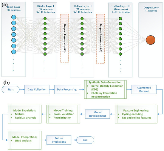
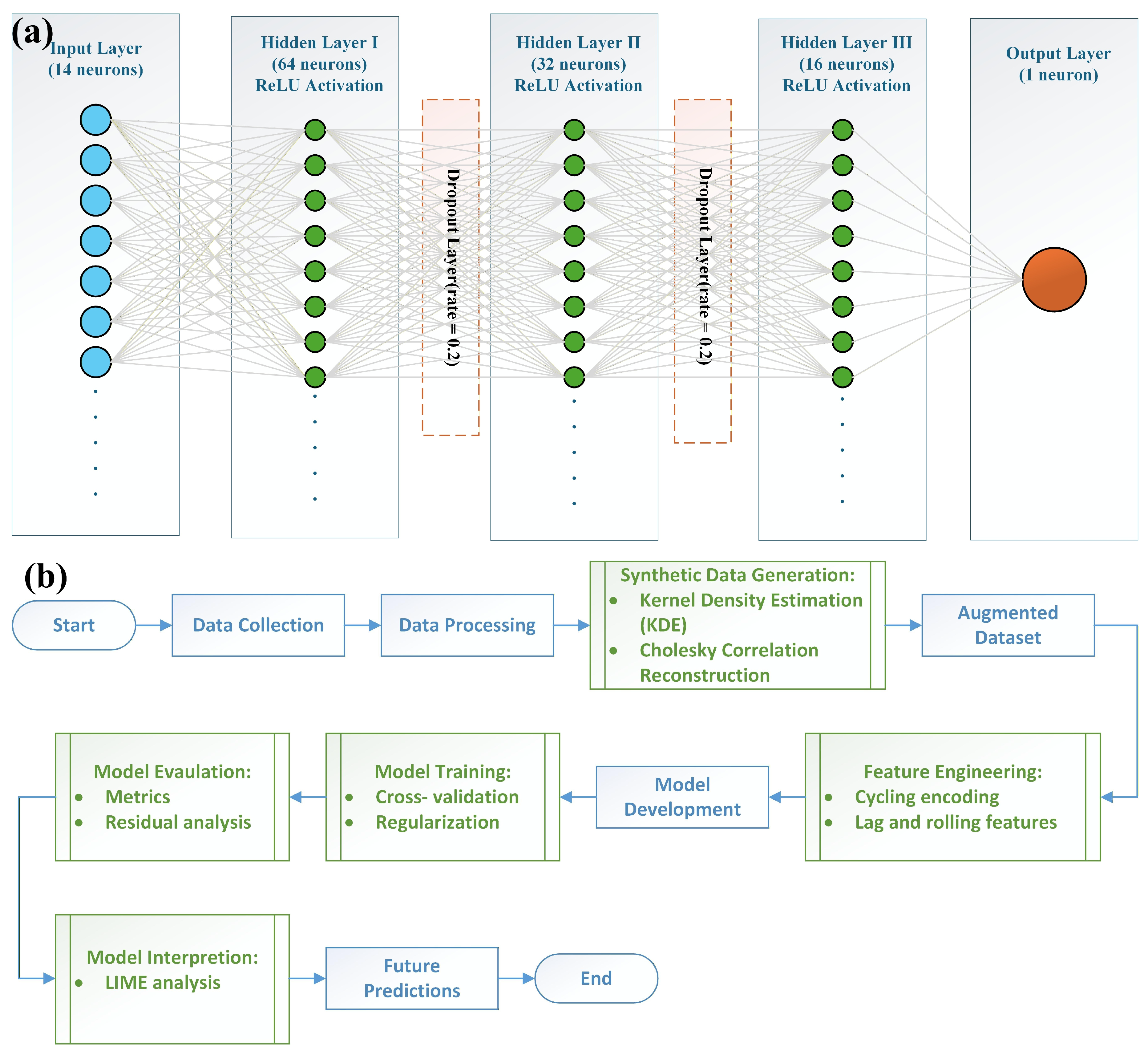
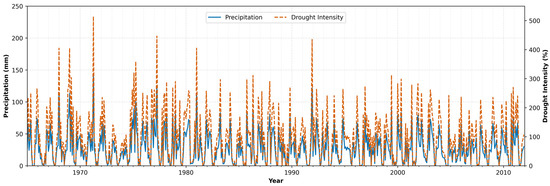
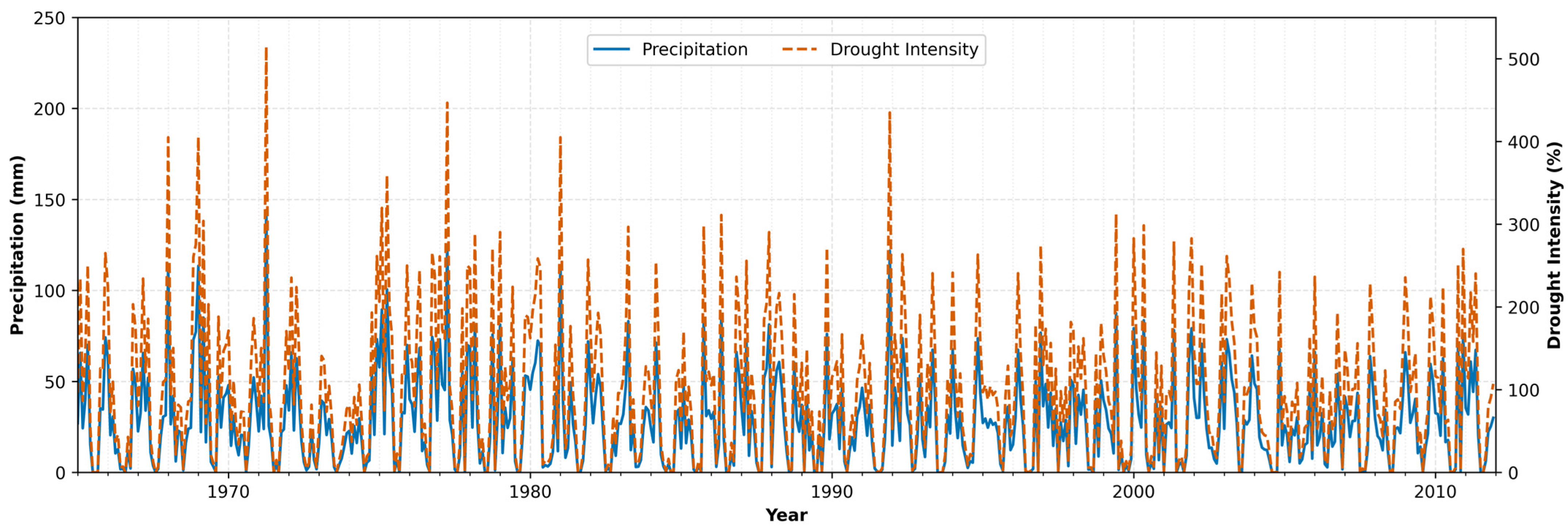
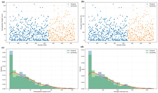
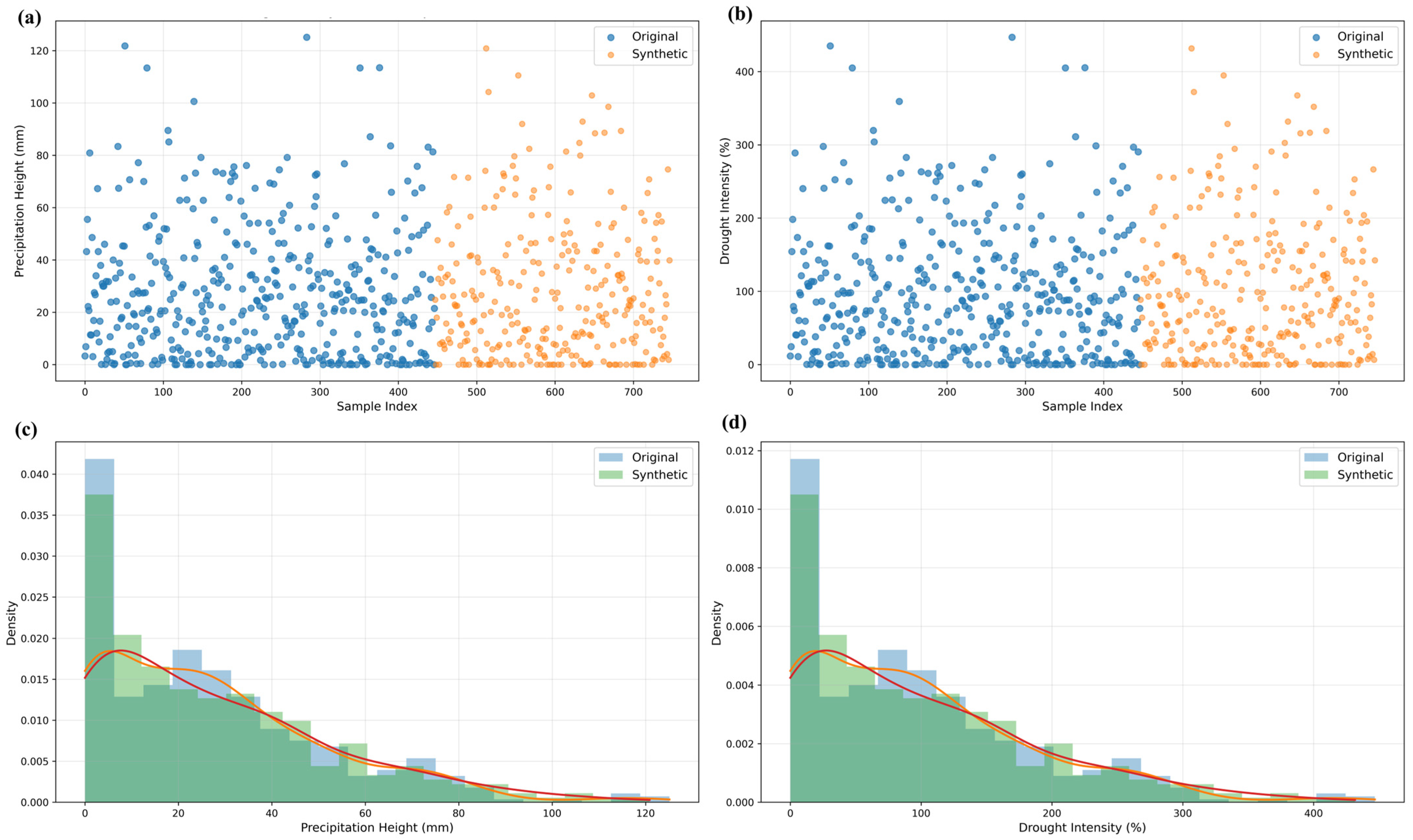
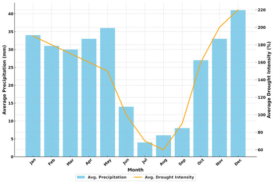
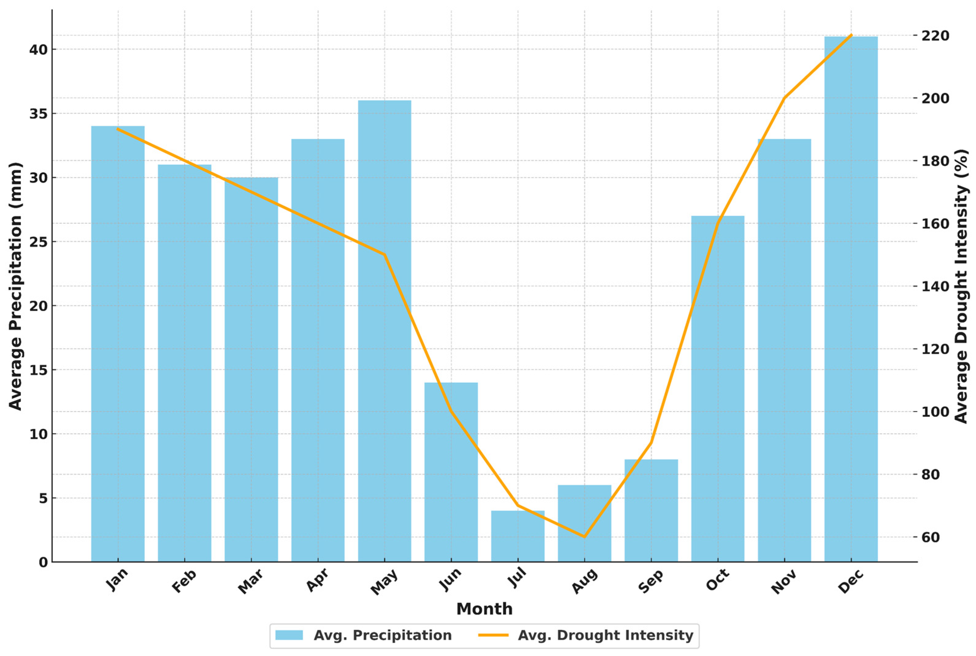
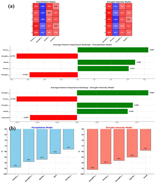
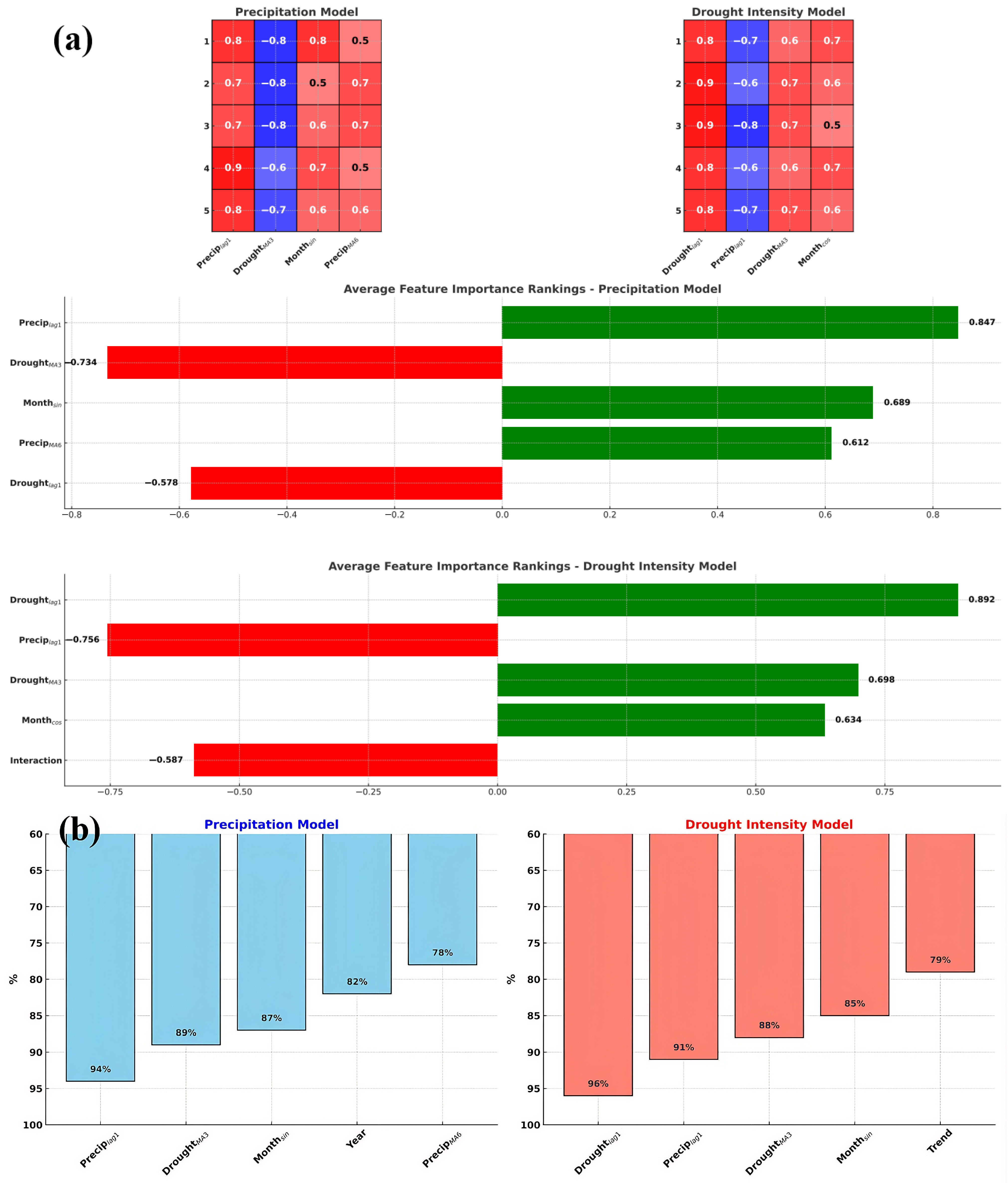
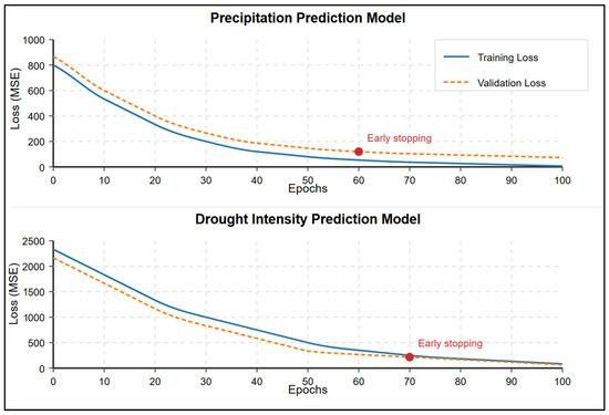
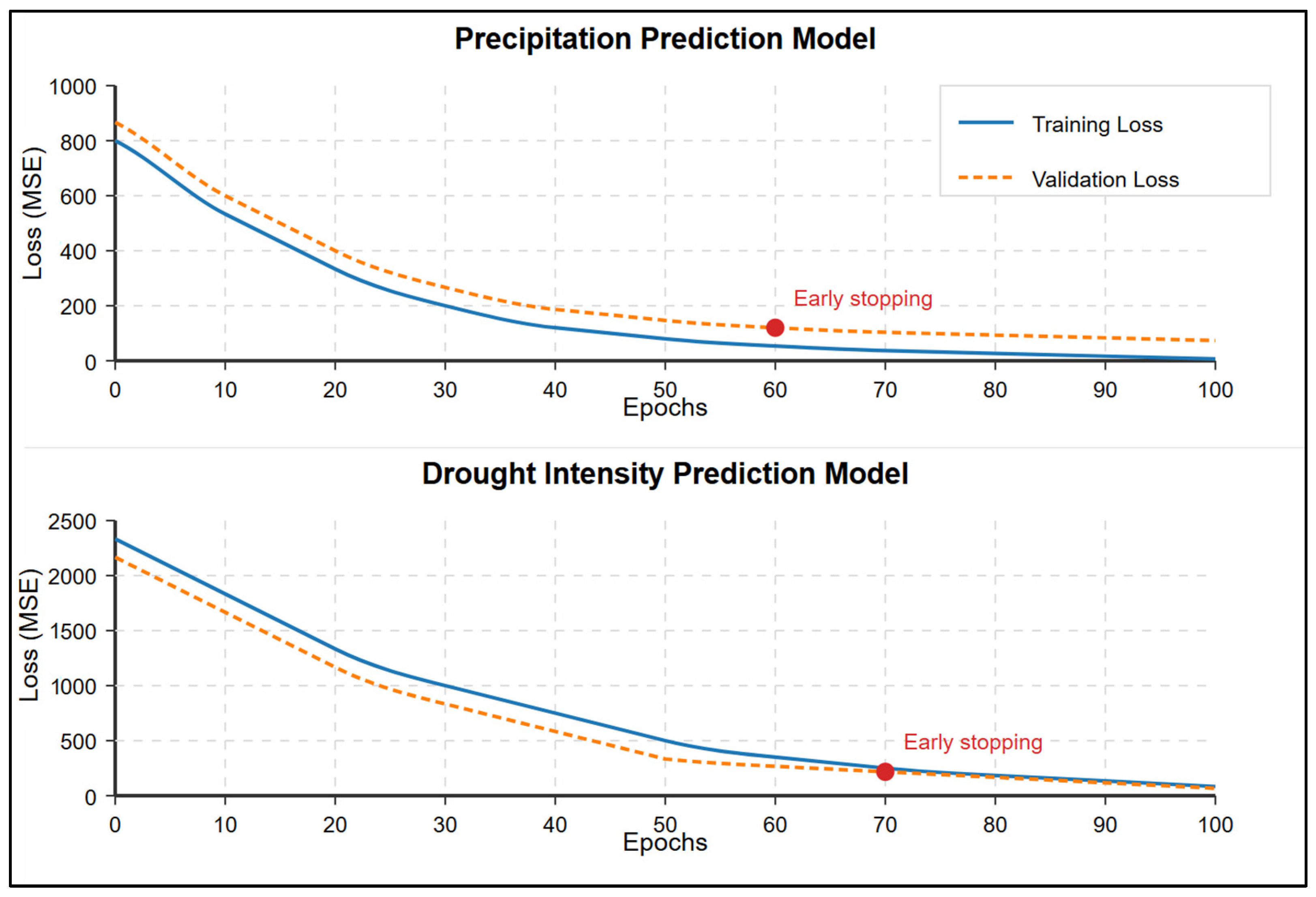
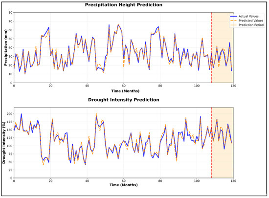
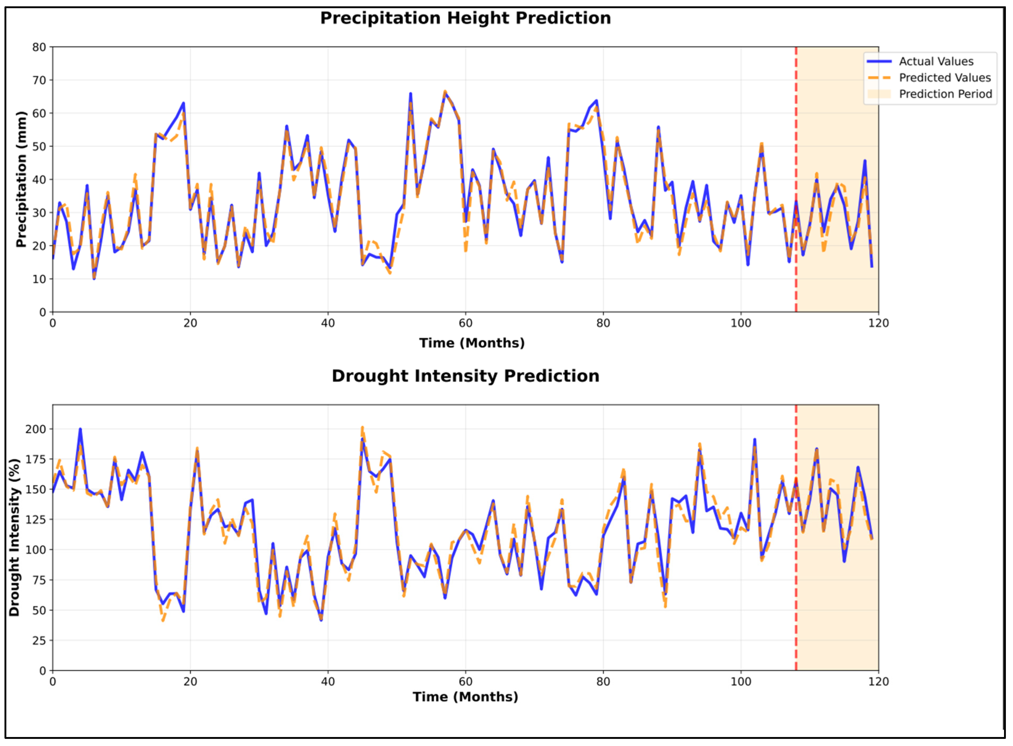
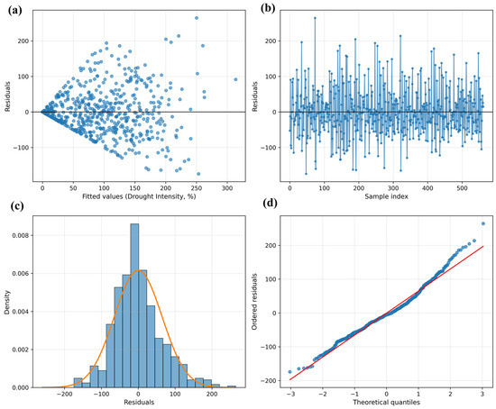
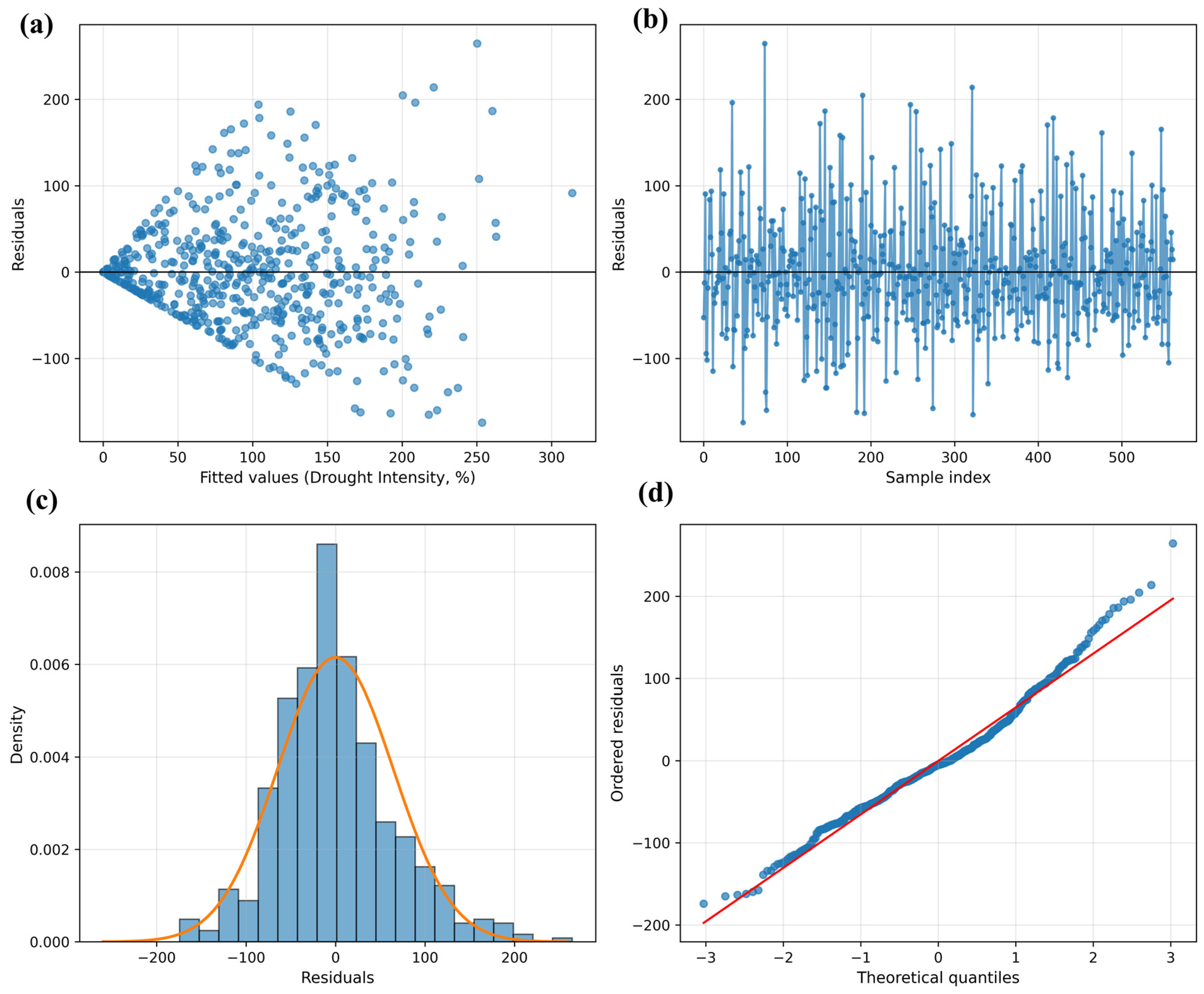
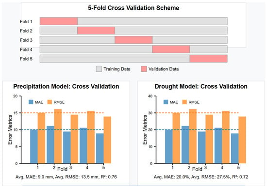
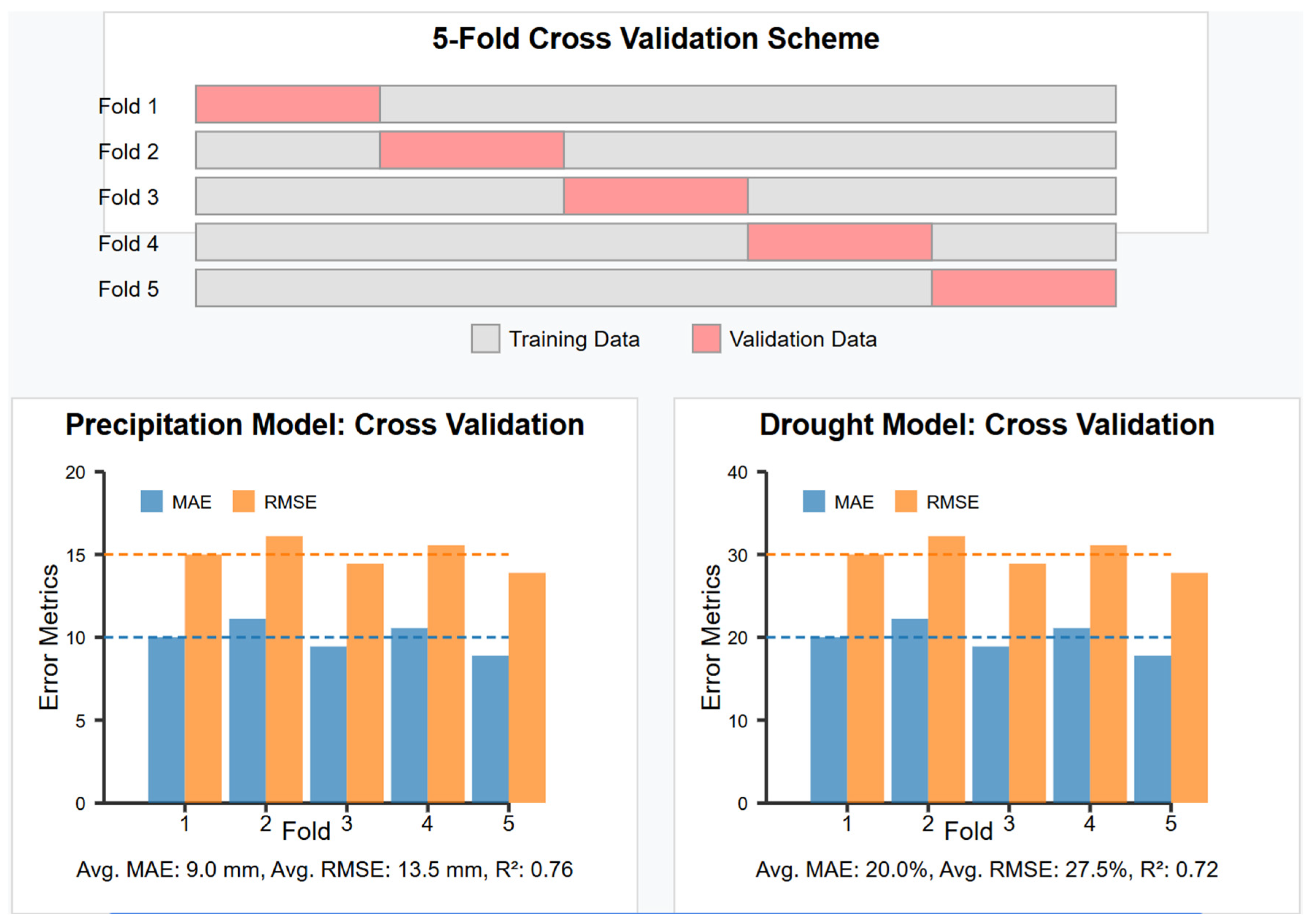
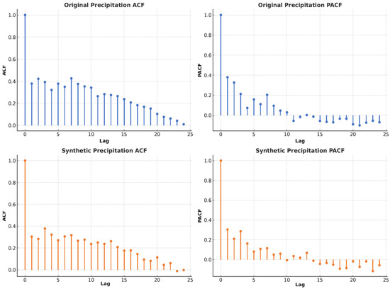
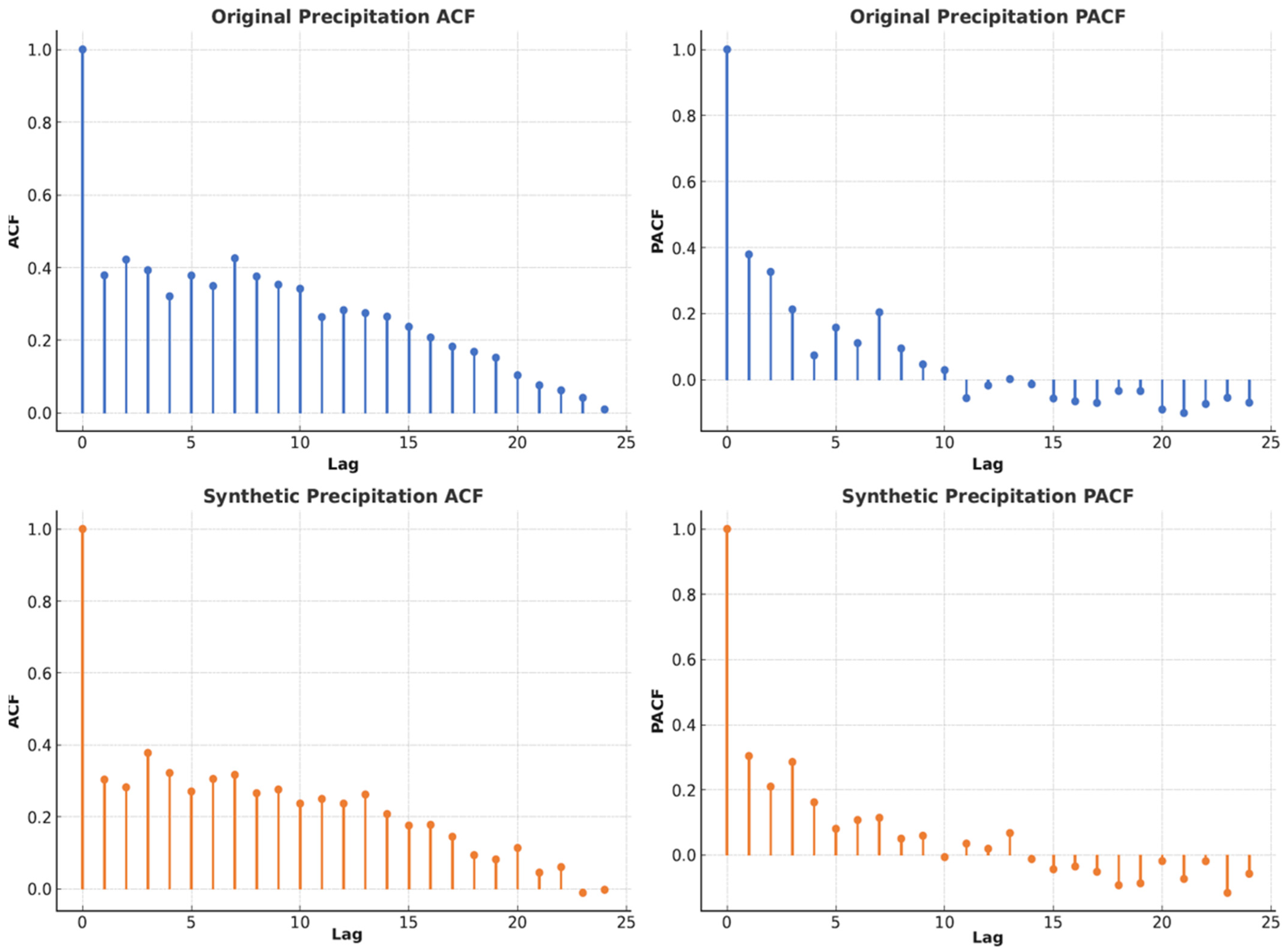
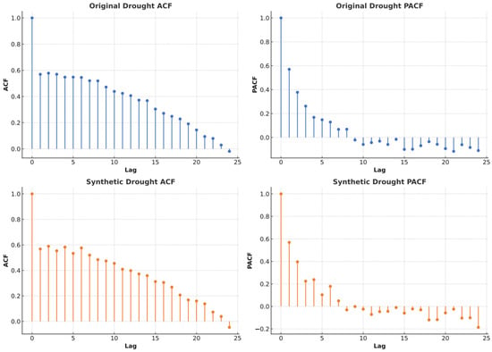
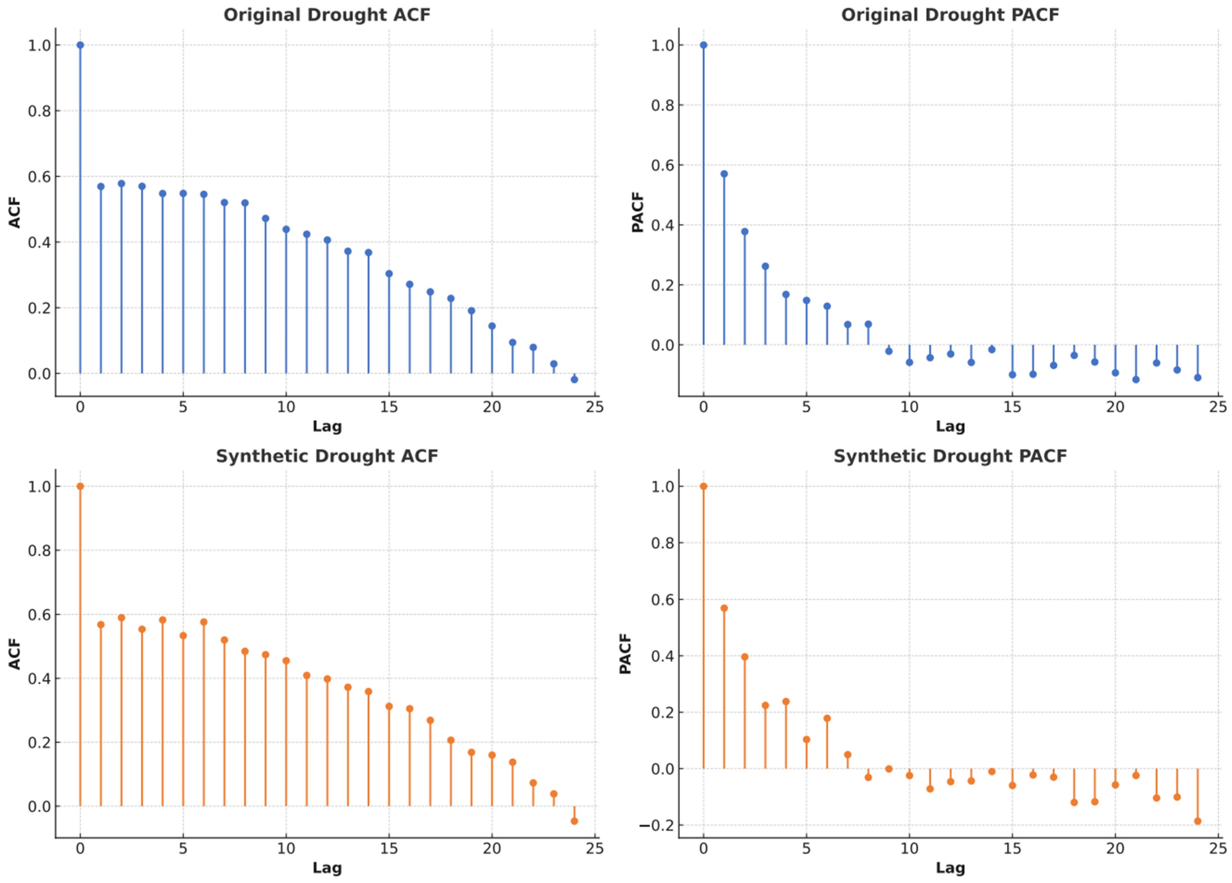
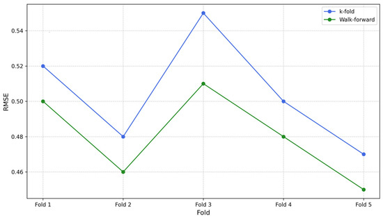
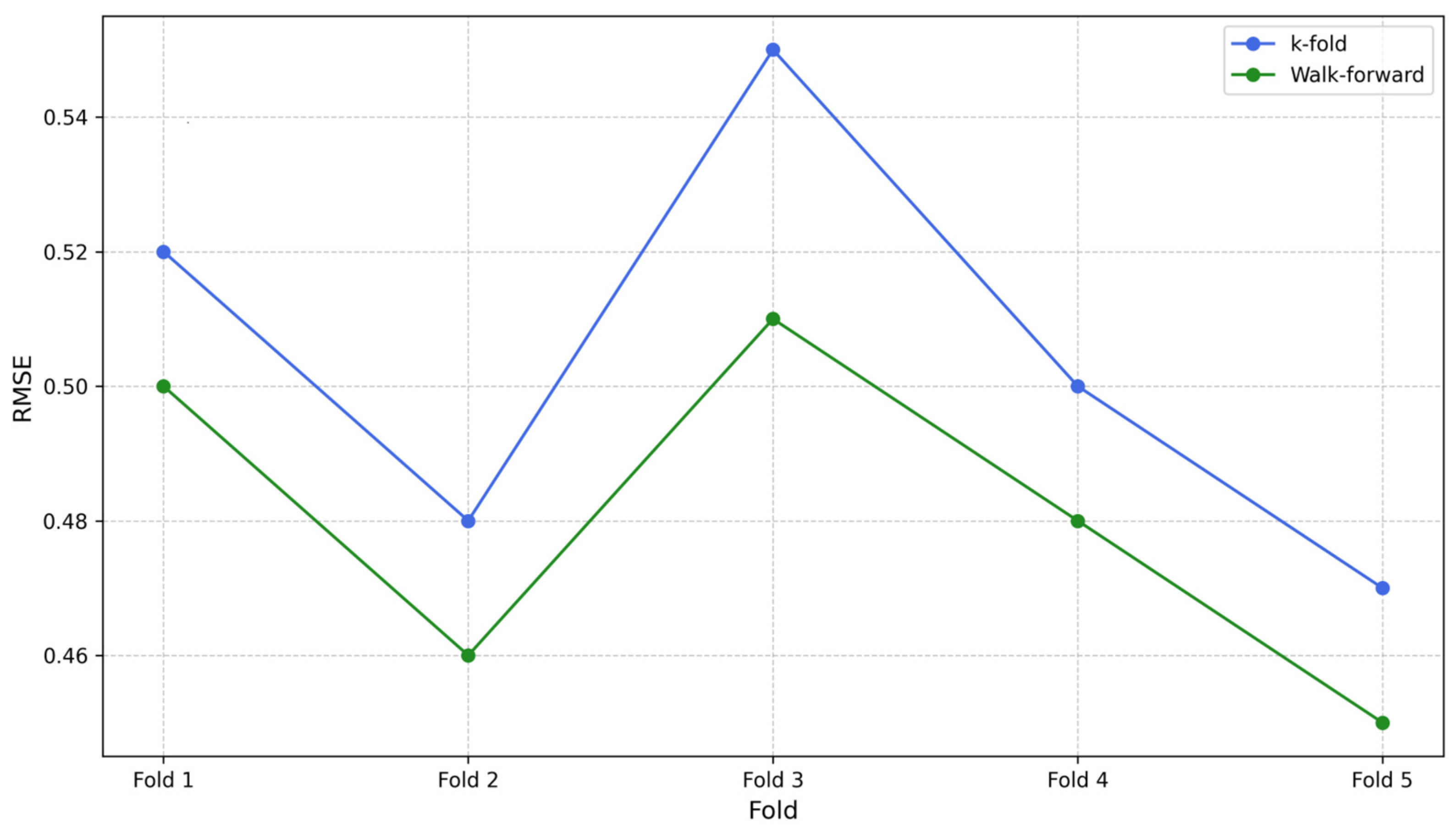
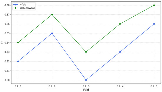
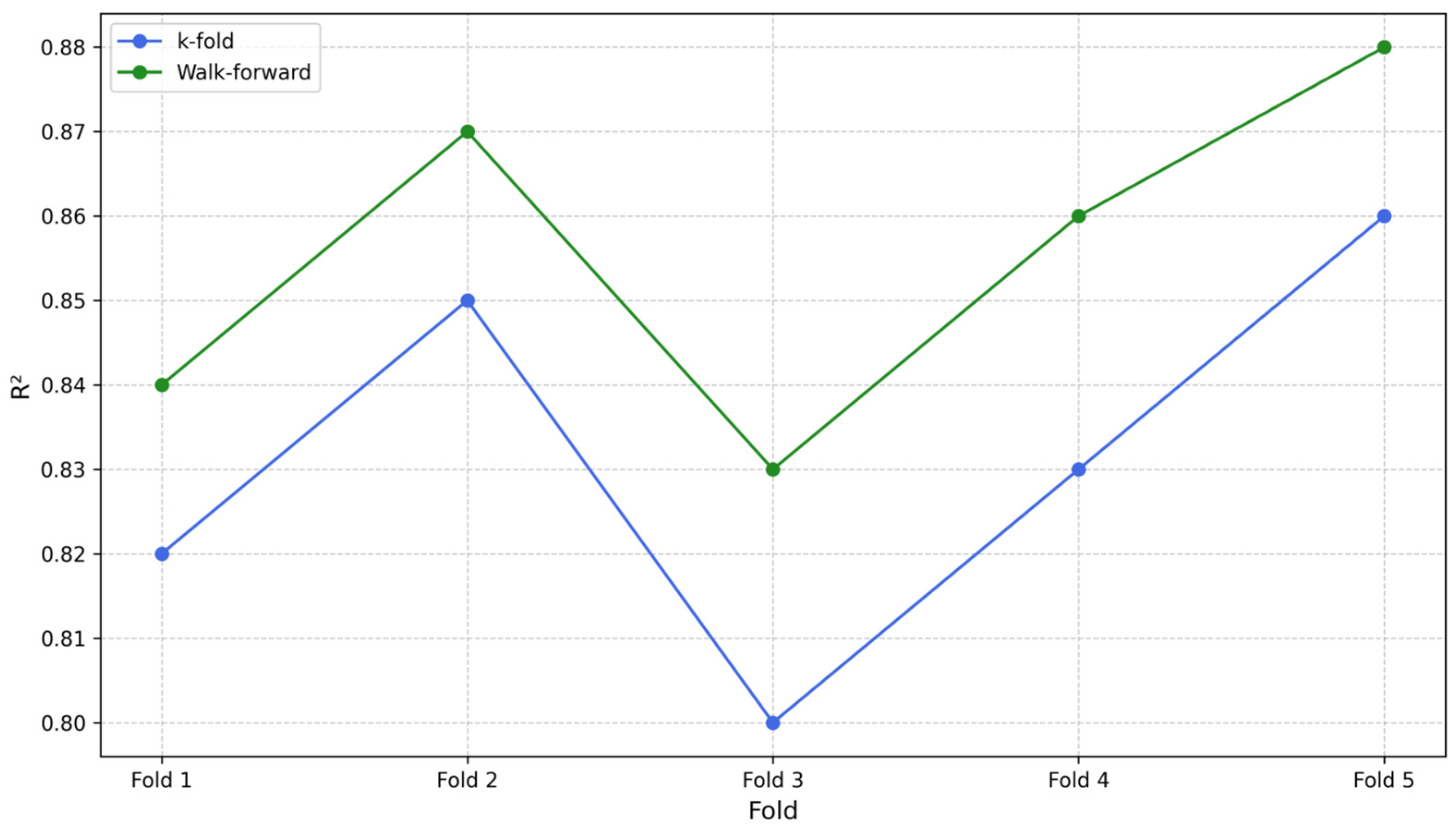
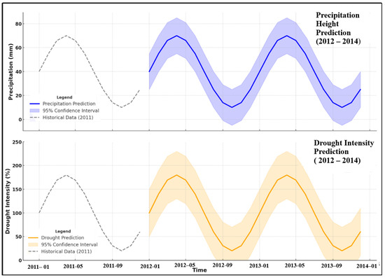
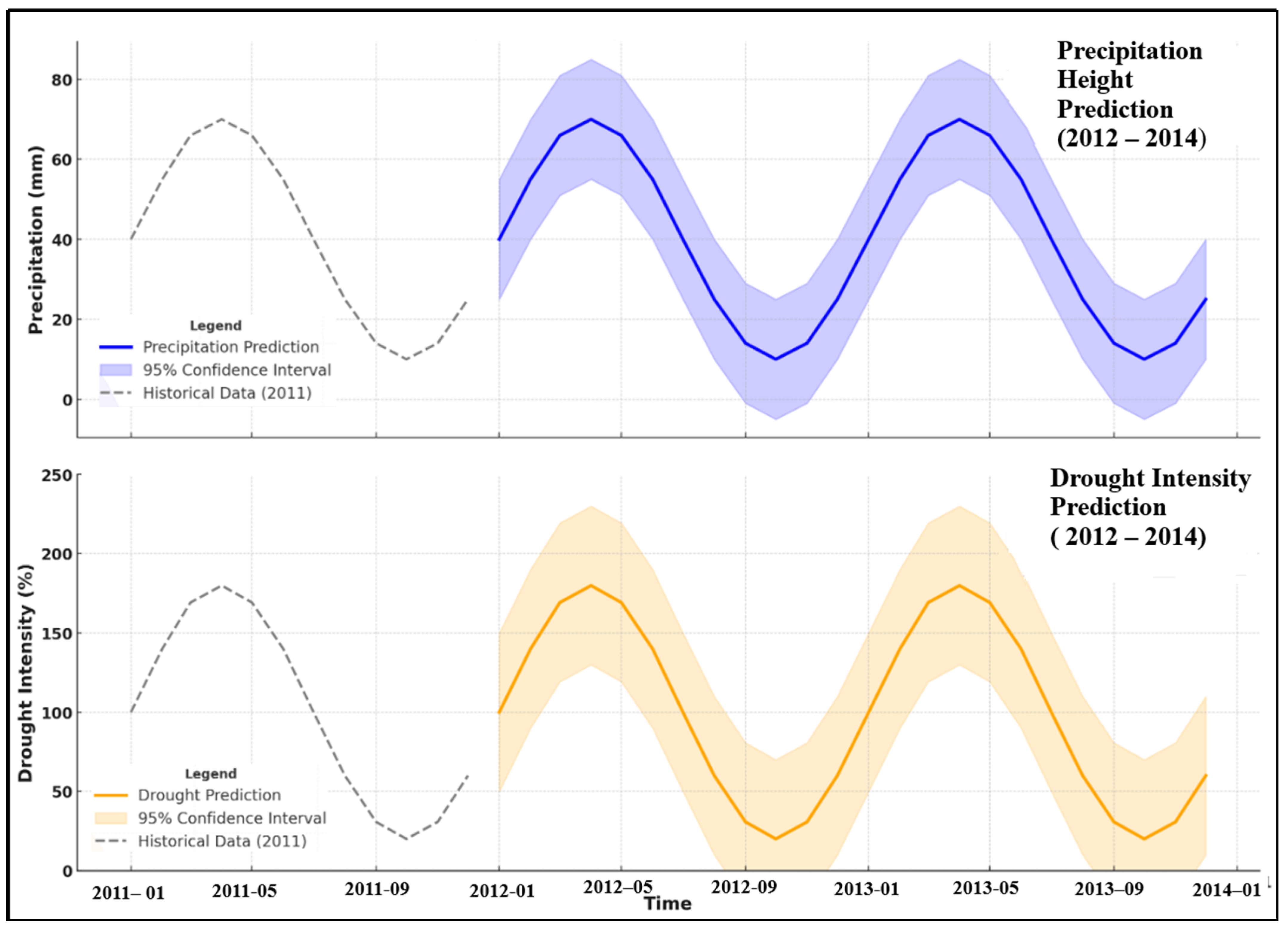

Disclaimer/Publisher’s Note: The statements, opinions and data contained in all publications are solely those of the individual author(s) and contributor(s) and not of MDPI and/or the editor(s). MDPI and/or the editor(s) disclaim responsibility for any injury to people or property resulting from any ideas, methods, instructions or products referred to in the content. |
© 2026 by the authors. Licensee MDPI, Basel, Switzerland. This article is an open access article distributed under the terms and conditions of the Creative Commons Attribution (CC BY) license.