


Abstract
Traditional leaf area index (LAI) measurement methods are destructive, time-consuming, and labor-intensive. In this study, 282 four-year-old central-leader apple trees were used as research subjects. Canopy reflectance spectra in the range of 4000–10,000 cm−1 were collected, and the corresponding true LAI values were measured destructively by harvesting all leaves from a representative branch of each tree using a leaf area meter. The dataset was randomly divided into training (70%) and testing (30%) sets. Eight spectral pretreatment methods were compared. The Competitive Adaptive Reweighted Sampling (CARS) algorithm was employed to extract characteristic wavelengths. Subsequently, both a BP neural network and a Support Vector Machine (SVM) model for LAI prediction were constructed. The optimal model was selected based on evaluation metrics including the coefficient of determination (R2), mean absolute error (MAE), mean bias error (MBE), and mean absolute percentage error (MAPE). The combined preprocessing of MSC and SD yielded the optimal results, screening out 26 characteristic wavelengths. The SVM linear kernel model (c = 5, g = 0.3) constructed based on MSC + SD preprocessing performed best, achieving a validation set R2 of 0.90, MAE of 0.2117, MBE of −0.1214, and MAPE of 16.09%. The performance on the training set and validation set was comparable, with no overfitting observed. The MSC + SD preprocessing combined with CARS feature screening and SVM linear kernel modeling enables rapid, non-destructive estimation of apple canopy LAI, providing an effective technical tool for precision orchard management.
1. Introduction
The leaf area index (LAI), defined as the total one-sided area of plant leaves per unit of ground surface area, is one of the most fundamental parameters for quantitatively describing canopy structure [1]. In studies on the cultivation physiology and ecology of apple (Malus domestica Borkh.), LAI not only determines the canopy’s capacity for light interception but also directly regulates the formation and distribution of photosynthetic products, as well as the spatiotemporal distribution of the orchard microclimate. Accurately quantifying LAI and its dynamic change is of significant scientific and practical value for elucidating the physiological mechanisms underlying high yield and quality in apple production and for optimizing tree architecture and cultivation management practices [2].
Traditional methods for LAI measurement primarily include the direct harvest method and optical instrument-based methods. The direct harvest method obtains the true LAI by collecting all leaves and measuring their area. Although it offers high accuracy, it is destructive, time-consuming, and labor-intensive, making it difficult to achieve fixed-point tracking and large-scale dynamic monitoring [3]. Optical instrument methods, such as the LAI-2000 plant canopy analyzer, estimate LAI by inverting radiation transfer models. While operationally more convenient, they are prone to systematic underestimation in the canopies of woody plants like apple due to leaf clumping effects. Reliable data typically require correction via destructive sampling [4]. The aforementioned methods all have certain limitations in terms of timeliness, repeatability, and spatial representativeness, making it difficult to meet the demands of modern precision orchard management for rapid, non-destructive acquisition of LAI information [5].
Near-infrared spectroscopy offers a new technical approach for the non-destructive monitoring of canopy parameters in fruit trees [6]. The spectral reflectance in the near-infrared band (4000–10,000 cm−1, corresponding to wavelengths of 1000–2500 nm) [7] is highly sensitive to features such as canopy structure, internal leaf scattering, and leaf inclination angle, and exhibits a strong correlation with the leaf area index [8]. This band encompasses the characteristic absorption peaks of major chemical components within leaves, such as moisture, cellulose, and proteins. The combination and overtone absorption information from hydrogen-containing groups (C–H, N–H, O–H) in organic molecules can indirectly reflect the material accumulation and structural characteristics of the canopy [9]. Research has shown that the reflectance of apple canopies in the near-infrared region increases with rising LAI, providing a physical basis for the inversion of LAI using near-infrared spectral information [10].
In recent years, machine learning algorithms have demonstrated excellent nonlinear mapping capabilities and high prediction accuracy in the analysis of spectral data [11]. The BP neural network possesses strong self-learning and adaptive abilities, enabling it to approximate complex nonlinear relationships, which makes it suitable for handling the intricate associations between spectral data and agronomic parameters [12]. Support Vector Regression (SVR), based on the principle of structural risk minimization, exhibits good generalization performance in problems involving small sample sizes, nonlinearity, and high-dimensional pattern recognition [13]. Integrating these algorithms with near-infrared spectroscopy technology offers new possibilities for the accurate estimation of apple tree LAI.
This study aims to establish a rapid, non-destructive LAI estimation method for apple canopies using a portable Fourier Transform Near-Infrared Spectrometer (Thermo Fisher Scientific, Waltham, MA, USA) combined with machine learning, supporting precision orchard management.
2. Materials and Methods
2.1. Site Overview and Experimental Materials
This experiment was conducted in an apple orchard located in Tamen Town, Alar City. The test material consisted of four-year-old apple trees planted with a spacing of 1.8 m × 3.5 m in an east–west row orientation, trained to a central leader fruiting system. The average tree height was 3.5 m, with a canopy diameter ranging from 1.25 m to 1.75 m, and the working alley width was 3.5 m. Because the row spacing (3.5 m) was larger than the canopy diameter (max. 1.75 m), the inter-row space remained open, and canopies of adjacent rows did not touch each other. Although canopies of neighboring trees within the same row overlapped slightly, they did not form a continuous closed canopy. Therefore, the leaf area index (LAI) measurements in this study were performed on individual tree canopies rather than on a closed canopy. The orchard soil was classified as sandy loam, and the terrain was flat. A total of 282 sample trees exhibiting normal growth, free from mechanical damage and significant pests or diseases, were selected. For canopy spectrum collection, 12 measurement points were marked on each sample tree, corresponding to four cardinal directions (east, south, west, north) and three vertical layers (upper, middle, lower) [14]. For LAI measurement using the LAI-2000 Plant Canopy Analyzer, a separate protocol was applied: 5–8 measurement points were arranged in a grid pattern within the vertical projection area of each tree canopy (avoiding the trunk and bare inter-row ground). The probe was fitted with a 90° view cap, with the shading direction aligned parallel to the tree rows to minimize the influence of adjacent canopies and direct sunlight. The study employed a field experimental design and was conducted in conjunction with statistical analysis methods.
2.2. Canopy Spectral Data Acquisition
In late August 2024, canopy spectral scanning was conducted using an Antaris II Fourier Transform Near-Infrared Spectrometer (Thermo Fisher Scientific, Waltham, MA, USA) equipped with a fiber-optic diffuse reflectance probe (sampling spot diameter approximately 2 cm; field of view: 25°) [15]. The key instrument parameters were set as follows: spectral range 4000–10,000 cm−1, resolution 8 cm−1, with each spectrum being the average of 64 scans and recorded in reflectance format [16].
Measurements were performed under clear, cloudless conditions between 10:00 and 15:00, with wind speeds below force 3 on the Beaufort scale to ensure uniform and stable canopy illumination. The instrument was preheated for 30 min prior to measurement. A reference spectrum was collected using a standard diffuse reflectance white panel (Spectralon, reflectance > 99%), with recalibration performed every 30 min. A dark spectrum was also collected concurrently to subtract background noise. During measurement, the fiber-optic probe was held vertically above the leaf canopy, maintaining a distance of 5–10 cm from the leaf surface to ensure that the sampling spot fully covered the leaf area. At each marked point on every sample tree, three spectra were collected in succession, and their average was taken as the spectral data for that point. After every two to three sample trees, a white reference correction was repeated to mitigate instrument drift [17].
To verify the quality of the acquired spectral data, the reflectance curves of the apple canopies were examined. As shown in Figure 1a, the original spectral reflection characteristics within the wavenumber range of 4000–10,000 cm−1 exhibited the typical near-infrared reflectance pattern of a healthy apple canopy reported in the literature [18,19] Specifically, the reflectance showed a gradual upward trend from 4000–5000 cm−1; a relatively stable plateau between 5000 and 7000 cm−1 with a weak absorption feature around 6800–7200 cm−1 (corresponding to the O–H combination band of leaf moisture, with a typical peak near 6900 cm−1); and a continued rise from 7000 to 10,000 cm−1, leveling off after 9000 cm−1. These features confirm that the collected spectra are of sufficient quality for subsequent analysis. The high reflectance in the near-infrared shortwave region originates from multiple scattering of light by intercellular air spaces within the leaf, the absorption in the near-infrared longwave region is primarily controlled by leaf moisture content, and the canopy structure (e.g., leaf area index, leaf inclination angle) modulates the overall intensity and directionality of these signals at the population scale. The observed variations in reflectance across different wavenumbers reflect spatial heterogeneity in canopy structure and leaf area index among sampling points or canopy sections. Therefore, these original spectral data provide a reliable foundation for the subsequent extraction of characteristic wavelengths and the construction of a leaf area index prediction model.
Figure 1.
Near-infrared original spectrum and leaf area index statistics: (a) visualization of the original spectrum; (b) visualization of leaf area index statistics.
2.3. Leaf Area Index Measurement
In late August 2024, the leaf area index (LAI) of apple tree canopies was measured using an LAI-2000 Plant Canopy Analyzer (LI-COR, Lincoln, NE, USA). In this study, LAI refers specifically to the green leaf area index. Measurements were conducted under diffuse light conditions during the peak fruiting period (late July to late August). The probe was fitted with a 90° view cap, with the shading direction aligned parallel to the tree rows. For each treatment, 12 representative sample trees were selected. Within the canopy of each tree, 5 to 8 measurement points were arranged in a grid pattern below the canopy to collect below-canopy (B) readings, while above-canopy (A) readings were simultaneously collected in an open area above the canopy. The instrument automatically recorded radiation transmittance at five zenith angles (7°, 23°, 38°, 53°, and 68°) and calculated LAI based on Miller’s theory. Three replicate measurements were taken per tree, and the average value was used as the LAI for that tree [20].
To correct the underestimation of green LAI caused by leaf clumping in the optical method (approximately 32.0% in high-density orchards), all leaves from three standard trees within each treatment were simultaneously collected. Only healthy green leaves were retained after removing senescent, yellow, diseased, or non-green leaves. The area of each single green leaf was measured using an LI-3100 leaf area meter to calculate the total green leaf area per tree, and the direct green LAI was then derived. A regression equation was established between the optical LAI and the direct green LAI, and all measured optical LAI values were corrected accordingly, as shown in Equation (1) [21].
Ltrue represents the corrected LAI, while Leff denotes the uncorrected LAI. The parameters a and b were derived by fitting destructive sampling data obtained from the same orchard.
2.4. Spectral Data Transformation
Raw near-infrared spectroscopy (NIR) spectra are susceptible to interference from environmental noise, light scattering effects, and baseline drift, which can reduce prediction accuracy if used directly for modelling [22]. To mitigate these interferences and improve the signal-to-noise ratio, this study applied a series of pretreatment transformations to the collected raw reflectance spectra from the apple canopy. This process derived nine spectral data types: raw reflectance (R), multiplicative scatter correction (MSC), Smooth, first derivative (FD), second derivative (SD), and their combined forms: MSC + FD, MSC + SD, Smooth + FD, and Smooth + SD.
Multiplicative scatter correction (MSC) corrects for both additive and multiplicative effects between each spectrum and a reference spectrum (typically the mean spectrum) through linear regression. This method effectively eliminates baseline offset and tilt caused by uneven particle distribution and surface scattering in samples. It enhances spectral reproducibility and the signal-to-noise ratio, thereby allowing the spectra to more accurately reflect the contribution of the sample’s chemical composition [23]. Smooth processing (Smooth) employs a sliding window average or weighted average to filter spectral data. This can suppress random noise while largely preserving the main spectral features. The selection of the window width requires a balance between noise reduction and signal distortion [24].
Derivative processing can effectively separate overlapping peaks and eliminate baseline interference. The first derivative (FD) can remove constant baseline offset and linear drift, highlighting changes in spectral slope and enhancing band features, which aids in distinguishing adjacent absorption peaks [25]. The second derivative (SD) is more sensitive to spectral curvature and can further resolve the fine structure of overlapping peaks, identifying shoulders and inflection points. However, it amplifies high-frequency noise and is therefore typically used in combination with smoothing methods [26].
In this study, all derivative calculations were performed using the Savitzky–Golay convolutional method with a second-order polynomial and a 7-point window. The same parameters were applied for both FD and SD. Combined preprocessing aims to integrate the advantages of individual methods. MSC + FD first corrects for scattering interference using MSC (implemented via the standard multiplicative scatter correction algorithm), then employs the Savitzky–Golay FD to eliminate residual baseline drift and enhance spectral band resolution. This approach is suitable for samples with significant scattering effects requiring precise peak positioning. MSC + SD introduces the second derivative (SD) on the basis of MSC, enabling more sensitive detection of subtle variations in highly overlapping peaks. It is thus appropriate for analyzing spectra from samples with complex compositions [27]. Smooth + FD first applies a Savitzky–Golay smoothing filter (same polynomial order and window size as above) to the spectrum to reduce noise, followed by calculation of the first derivative. This effectively prevents noise amplification during differentiation, balancing noise suppression with feature enhancement. Smooth + SD also performs smoothing prior to differentiation; the second derivative can more reliably reflect changes in spectral curvature and reduce the risk of false peaks. This method is particularly suited for scenarios where the original spectrum has a high noise level and fine structure analysis is required [28].
All preprocessing steps were carried out in MATLAB R2024b (MathWorks, Inc., Natick, MA, USA). Specifically, the sgolay function was used for Savitzky–Golay smoothing and derivative calculation; MSC was implemented with an in-house script following the standard algorithm (mean spectrum as reference); smoothing was also performed using sgolay with the same window and polynomial order.
2.5. Spectral Feature Band Extraction
The full spectral band contains a large volume of data with substantial collinearity and redundant information. To simplify the model, improve computational efficiency, and enhance the model’s generalization ability, this study employed the Competitive Adaptive Reweighted Sampling (CARS) algorithm to screen the characteristic wavelength variables most relevant to LAI values from the pretreated spectra. Through adaptive weighted sampling and a competitive mechanism, the CARS algorithm iteratively selects wavelength points with larger absolute values of regression coefficients, thereby optimizing a characteristic wavelength subset with strong representativeness and significantly reducing data dimensionality [29].
2.6. Model Construction and Validation
In constructing the Support Vector Regression (SVR) model, a comparative analysis was conducted using four kernel functions: the Radial Basis Function (RBF), the linear kernel function, the polynomial kernel function, and the Sigmoid kernel function. The grid search method was employed to optimize the penalty parameter c (with values of 0.1, 0.5, 1, 5, and 10) and the RBF kernel function parameter γ (with values of 0.01, 0.03, 0.1, and 0.3), in order to determine the optimal parameter combination for each kernel function [30].
The BP neural network adopted a three-layer topology comprising an input layer, a single hidden layer, and an output layer. The search range for the number of nodes in the hidden layer was set from 5 to 15. The network training parameters were configured as follows: the maximum number of iterations was 1000, the learning rate was 0.01, and the training target error was 1 × 10⁻⁶. To determine the optimal training algorithm, six training functions were compared and analyzed: trainlm, traingd, trainscg, traingdx, trainbfg, and traincgb. Through experimentation, the optimal combination of the number of nodes in the hidden layer and the training function was screened out [31].
Data pretreatment and partitioning: The data were standardized using Z-score normalization Equation (2) and then randomly split into a training set (70%) and a validation set (30%) [32].
where Q is the raw measurement data, Qn is the standardized value of the raw measurement data, and Qmax and Qmin are the maximum and minimum values of the variable, respectively.
Model Training and Evaluation: The model performance was comprehensively assessed using the coefficient of determination (R2, Equation (3)), mean absolute error (MAE, Equation (4)), mean absolute percentage error (MAPE, Equation (5)), and model bias error (MBE, Equation (6)) [33].
2.7. Feature Importance Analysis and Model Optimization
All testing data were subjected to descriptive statistics and Pearson correlation analysis using Origin 2021. Neural network modeling and related computations were completed in the MATLAB R2024b environment.
3. Results and Analysis
3.1. Leaf Area Index Analysis
Figure 1b shows the distribution of the leaf area index (LAI) sampled from the apple tree canopy. LAI is a core parameter characterizing canopy structure, photosynthetic potential, and biomass production capacity. Regarding the distribution pattern, the sample LAI values show a relatively concentrated distribution, primarily within the range of 1.0 to 2.0. The count peaks occur at LAI = 1.0 and LAI = 2.0, indicating that the canopies of the samples in this study are predominantly of medium to low closure density [34]. The sample number with an LAI below 1.0 was relatively small (corresponding to smaller trees or plants with canopies not yet fully closed), and the number of samples with high canopy closure (LAI ≥ 3.0) was also limited. This aligns with the actual condition of the test materials, which were four-year-old central-leader apple trees whose canopies were still in a developmental stage. This distribution indicates a degree of natural variation in the canopy structure among the apple tree samples used in the trial. Furthermore, the samples are predominantly representative of the canopy state at a specific phenophase (late August) and tree age, characterized by an LAI of 1.0–2.0, making them suitable for establishing a spectral prediction model for leaf area index.
In summary, this study successfully acquired spectral reflectance data in the 4000–10,000 cm−1 near-infrared band from apple tree canopies, along with their corresponding measured LAI values. The canopy spectrum exhibits features in the near-infrared region associated with moisture absorption and canopy structure, while the LAI values are predominantly concentrated within the 1.0–2.0 range, indicating good sample representativeness. This is consistent with the existing literature [35], confirming the healthy physiological status of the plants. Therefore, based on the spectral data shown in Figure 1a, modelling approaches including feature selection and machine learning can be further employed to explore the quantitative relationship with the LAI values presented in Figure 1b. This will ultimately enable rapid, non-destructive spectral estimation of the leaf area index in apple tree canopies.
3.2. Spectral Preprocessing
This study employed multiplicative scatter correction (MSC), smoothing (Smooth), first derivative (FD), second derivative (SD), and their combined strategies (MSC + FD, MSC + SD, Smooth + FD, Smooth + SD) to preprocess the original reflectance spectra of the apple canopy. The aim was to enhance the spectral characteristics related to the leaf area index (LAI) while suppressing interfering factors such as environmental noise, scattering effects, and baseline drift.
The original reflectance spectra exhibited typical vegetation canopy reflection characteristics within the wavenumber range of 4000–10,000 cm−1. Due to limitations in field measurement conditions and the complexity of the canopy structure, the spectral curves displayed a certain degree of baseline drift and noise interference, which was particularly evident in the low wavenumber region of 4000–5500 cm−1. Following Multiplicative Scatter Correction (MSC) processing, the baseline shifts between spectral curves were effectively corrected, and the spectral overlap between different samples was significantly improved, indicating that the scattering effect was well suppressed (Figure 2a). After Smooth processing, the high-frequency noise in the spectral curves was markedly reduced, while the main absorption peak shapes were preserved, a result particularly evident in the 5500–7500 cm−1 region (Figure 2b). First Derivative (FD) processing accentuated the slope changes in the spectral curves, generating distinct alternating positive and negative peaks around 4000–5000 cm−1 and 6500–7000 cm−1, thereby enhancing the discernibility of LAI-related features (Figure 2c). Second Derivative (SD) processing further amplified the curvature changes of the spectrum, demonstrating greater sensitivity to the fine structure of overlapping peaks, which makes it suitable for extracting information features associated with low concentrations (Figure 2d). The combined preprocessing strategy demonstrated a synergistic optimization effect. MSC + FD not only eliminated scattering interference but also enhanced the dynamic features of the spectrum, making the spectral differences between samples with varying LAI more distinct (Figure 2e). MSC + SD achieved the dual advantages of scatter correction and fine-structure extraction. The processed spectra exhibited more regular peak shapes and stable baselines across multiple wavenumber intervals, providing high-quality input for identifying LAI-sensitive bands (Figure 2f). Smooth + FD reduced noise while highlighting the rate of change in the spectrum, effectively preventing the amplification of noise in the derivative results (Figure 2g). Smooth + SD balanced smoothing for noise reduction with the ability to resolve details. The processed spectra retained the main absorption features while showing more stable and reliable curvature changes (Figure 2h). A comprehensive comparison of the pretreatment effects revealed that the MSC + SD combination yielded the most significant optimization of the apple canopy spectrum in this study. This treatment effectively eliminated physical interference while maximizing the retention of subtle spectral characteristics related to canopy structure and LAI. Subsequently, characteristic wavelength bands will be extracted based on this pretreatment combination and integrated with machine learning algorithms to construct an LAI prediction model, aiming to achieve rapid and accurate estimation of the leaf area index in apple canopies.
Figure 2.
Visualization of spectral pretreatment: (a) the multiplicative scatter correction pretreatment algorithm; (b) the Smooth pretreatment algorithm; (c) the first derivative pretreatment algorithm; (d) the second derivative pretreatment algorithm; (e) the multiplicative scatter correction plus first derivative pretreatment algorithm; (f) the multiplicative scatter correction plus second derivative pretreatment algorithm; (g) the Smooth plus first derivative pretreatment algorithm; (h) the Smooth plus second derivative pretreatment algorithm.
3.3. Correlation Analysis Between Preprocessed Spectra and Leaf Area Index
This study evaluated the optimization effects of various methods on LAI-related spectral characteristics by analyzing the correlation coefficients (r) between different preprocessed spectra and the leaf area index (LAI) of apple canopies. The correlation curves for the eight pretreatment methods are shown in Figure 3a–h.
Figure 3.
Correlation between the preprocessed spectra and leaf SPAD content: (a) multiplicative scatter correction pretreatment algorithm; (b) Smooth pretreatment algorithm; (c) first derivative pretreatment algorithm; (d) second derivative pretreatment algorithm; (e) multiplicative scatter correction plus first derivative pretreatment algorithm; (f) multiplicative scatter correction plus second derivative pretreatment algorithm; (g) Smooth plus first derivative pretreatment algorithm; (h) Smooth plus second derivative pretreatment algorithm.
After MSC processing (Figure 3a), the spectrum exhibited broad positive and negative correlation peaks within the 3800–10,000 cm−1 range. A strong positive correlation (r ≈ 0.58) appeared near 3900 cm−1, and a strong negative correlation (r ≈ −0.52) appeared near 4300 cm−1. The overall peak shape was relatively gentle, indicating that scattering interference was partially corrected, but baseline drift persisted in some spectral bands. Such residual drift may introduce systematic errors into subsequent quantitative models, particularly affecting predictions at low LAI values where signal-to-noise ratios are lower. In this study, however, the subsequent second derivative (SD) processing applied after MSC effectively removed the remaining baseline drift, as evidenced by the superior performance of the MSC + SD combination (validation R2 = 0.90). For applications requiring long-term stability without derivative postprocessing, alternative preprocessing methods such as standard normal variate (SNV) or dedicated baseline correction algorithms (e.g., asymmetric least squares, iterative polynomial fitting) could be considered to address baseline drift more directly.
Smooth processing (Figure 3b) resulted in a monotonically decreasing negative correlation in the spectral correlation curve across the 4000–8500 cm−1 interval, with the r value gradually declining from −0.08 to −0.32. This demonstrates that smoothing can enhance low-frequency trends but may obscure local characteristic fluctuations. After FD processing (Figure 3c), the correlation curve exhibited high-frequency alternation between positive and negative values within the 4000–9500 cm−1 range. The r values mostly fluctuated between −0.4 and 0.4, reaching up to ±0.5 locally, reflecting the sensitivity of the first derivative to changes in spectral slope but also amplifying noise interference.
SD processing (Figure 3d) further amplified the spectral curvature changes. The correlation curve showed dense alternation of peaks and valleys in the 4000–10,000 cm−1 interval, with the fluctuation range of r values expanding to approximately ±0.4. While capable of revealing subtle structures, the noise level increased significantly, which is detrimental to stable modeling.
The MSC + FD combination (Figure 3e), building upon the scatter correction of MSC, enhanced dynamic features through the first derivative. The correlation curve displayed sharper positive and negative peaks within the 4000–9700 cm−1 range, for example, with r ≈ 0.50 at 4050 cm−1 and r ≈ −0.55 at 4200 cm−1. Although correlation improved in some bands, high-frequency noise remained quite pronounced. The MSC + SD combination (Figure 3f) achieved the dual advantages of scatter correction and fine structure extraction. The correlation curve exhibited clear and stable positive and negative correlation peaks within the 4000–10,000 cm−1 range, with peak values reaching ±0.6. Concurrently, noise was effectively suppressed, and the smoothness of the curve was significantly superior to that of the SD treatment alone, providing high-quality input for extracting LAI-sensitive bands.
The Smooth + FD combination (Figure 3g) involved derivation after smoothing for noise reduction. The correlation curve showed clear peaks and valleys in the 4000–9500 cm−1 interval, with r values fluctuating between −0.6 and 0.6. The noise level was reduced compared to the FD treatment alone, achieving a balance between noise suppression and feature enhancement.
The Smooth + SD combination (Figure 3h) applied second-order derivation after smoothing. The correlation curve displayed stable peak shapes within the 4000–10,000 cm−1 range, with the fluctuation range of r values narrowing to between −0.5 and 0.5. This approach effectively avoided false peaks while preserving subtle structures, making it suitable for fine analysis in high-noise environments. Based on a comprehensive comparison of the various preprocessing methods, the MSC + SD combination demonstrated the most significant effectiveness in this study. It maximally preserved the subtle spectral characteristics related to canopy structure and LAI while eliminating physical interference and maintained a low noise level, thereby establishing a reliable data foundation for the subsequent construction of a high-precision LAI prediction model.
3.4. Spectral Feature Extraction
This study employed the Competitive Adaptive Reweighted Sampling (CARS) algorithm to perform characteristic wavelength selection on the preprocessed near-infrared spectroscopy data of apple canopies. The aim was to extract effective information highly correlated with the Leaf Area Index (LAI), thereby reducing data dimensionality and optimizing the model input structure. The number of characteristic wavelengths retained after CARS screening for each preprocessing method is shown in Figure 4a–h.
Figure 4.
Feature extraction sites based on CARS for each set of preprocessed spectra: (a) the multiplicative scatter correction pretreatment algorithm; (b) the Smooth pretreatment algorithm; (c) the first derivative pretreatment algorithm; (d) the second derivative pretreatment algorithm; (e) the multiplicative scatter correction + first derivative pretreatment algorithm; (f) the multiplicative scatter correction + second derivative pretreatment algorithm; (g) the Smooth + first derivative pretreatment algorithm; (h) the Smooth + second derivative pretreatment algorithm.
The screening results for characteristic wavelengths varied significantly across different preprocessing methods. Only three characteristic wavelengths were selected after multiplicative scatter correction (MSC) preprocessing (Figure 4a), indicating that MSC effectively eliminated scattering interference, concentrating spectral information into a few core bands. Smooth preprocessing resulted in the selection of six characteristic wavelengths (Figure 4b). This method retained the primary trend information based on noise reduction through smoothing, yielding a relatively limited but highly representative set of features. The first derivative (FD) pretreatment method selected four characteristic wavelengths (Figure 4c). The sensitivity of the first derivative to changes in spectral slope resulted in the screening focusing on a limited number of bands with pronounced variations, leading to highly concentrated features. The second derivative (SD) pretreatment method selected 44 characteristic wavelengths (Figure 4d). The amplifying effect of the second derivative on spectral curvature changes caused numerous subtle fluctuations to be identified as potential features, significantly increasing the number of features. However, it is important to note that this may include false features induced by noise.
Notably, both MSC + SD and Smooth + SD preprocessing methods yielded exactly 26 characteristic wavelengths, reflecting a stable core spectral signal that is robust to different preprocessing strategies. Further analysis of the selected variables reveals that the two methods share several key common spectral bands, primarily distributed in three regions: The ~5200–5500 cm−1 region, which corresponds to the combination band of O-H stretching and bending vibrations, typically associated with water or hydroxyl-containing compounds; the ~7100–7300 cm−1 region, related to the first overtone of O-H stretching vibrations, a common marker for moisture or hydroxyl groups in organic materials; and the 8000–10,000 cm−1 region, which contains multiple selected variables corresponding to the second overtones of C-H stretching vibrations (e.g., in methyl and methylene groups), reflecting the organic composition of the samples.
The consistent selection of these chemically meaningful bands by both methods confirms that the combined preprocessing strategies effectively captured the key structural information relevant to the target property. While MSC + SD preserves fine spectral details and subtle variations, and Smooth + SD offers enhanced noise suppression, both methods ultimately converged on the same set of core chemical signals, highlighting the reliability of the selected features.
The differences in the number of characteristic wavelengths reflect the influence of different preprocessing methods on the distribution of spectral information. SD and its related combinations selected a larger number of features, which may contain richer structural details and help capture subtle variations related to LAI but require vigilance against overfitting risk. Preprocessing methods such as MSC and FD selected fewer features, with information being highly concentrated, which is beneficial for constructing concise and robust models. Overall, both MSC + second derivative and Smooth + second derivative achieved a favourable balance between the number of features and the quality of information, providing reliable feature inputs for the subsequent construction of the LAI prediction model in this study.
3.5. Apple LAI Prediction Model
3.5.1. Optimal Models Under Various Machine Learning Algorithms for the BP Neural Network
This study developed BP neural network models to predict apple canopy leaf area index (LAI) using eight spectral preprocessing methods (MSC, Smooth, FD, SD, MSC + FD, MSC + SD, Smooth + FD, Smooth + SD). For each method, the optimal model (varying hidden layer nodes from 5 to 15 and six training functions) was selected and evaluated using R2, MAE, MBE, and MAPE (see Table 1; detailed parameters in Supplementary Materials).
Table 1.
Performance metrics of the best models under each machine learning algorithm for the BP neural network.
Model performance varied considerably. MSC (MSC-6, trainbfg) achieved training/validation R2 of 0.92/0.88, with validation MAE = 0.178 and MAPE = 12.27%, indicating a good fit but moderate generalization. Smooth (Smooth-13, trainlm) gave balanced R2 (0.89/0.89) but higher errors (MAE = 0.2202, MAPE = 18.31%). FD (FD-6, trainlm) showed overfitting (R2 = 0.90/0.84, MAPE = 26.60%). SD (SD-7, trainscg) performed poorly (validation R2 = 0.81, MAE = 0.3079, MAPE = 20.95%). Among combined methods, MSC + FD (MSC + FD-7, trainlm) was superior to single methods (validation R2 = 0.85, MAPE = 15.39%) but was outperformed by MSC + SD. The MSC + SD-11 model (trainbfg) delivered the best results: training/validation R2 = 0.93/0.92, validation MAE = 0.207, MAPE = 14.26%, with minimal overfitting and strong generalization. Smooth + FD (Smooth + FD-11, trainscg) gave moderate accuracy (validation R2 = 0.85, MAPE = 19.81%), while Smooth + SD (Smooth + SD-5, trainlm) failed (validation R2 = 0.66, MAE = 0.4172), making it unsuitable for LAI estimation.
In summary, the MSC + SD-11 model exhibits the highest validation R2 (0.92) and lowest errors (MAE = 0.207, MAPE = 14.26%) without significant overfitting, effectively capturing subtle spectral features related to canopy structure and LAI. Therefore, it is identified as the optimal BP neural network model for predicting apple canopy LAI.
3.5.2. Optimal Models with Varying Numbers of Hidden Layers Under the BP Neural Network MSC Plus SD Algorithm
This study developed a BP neural network model for predicting apple canopy leaf area index (LAI) using spectral data preprocessed with multiplicative scatter correction (MSC) and second derivative (SD). Model parameters (hidden layer nodes 5–15, six training functions) were optimized based on R2, MAE, MBE, and MAPE (Table 2; detailed parameters in Supplementary Materials).
Table 2.
Optimal model metrics for different numbers of hidden layers under the BP neural network algorithm with MSC and SD.
As shown in Table 2, the MSC + SD-11 model (11 hidden nodes, trainbfg) performed best, with validation set R2 = 0.92, MAE = 0.207, MBE = 0.0246, and MAPE = 14.26%. Training set metrics (R2 = 0.93, MAE = 0.1698) were similar, indicating no significant overfitting and strong generalization.
Other models showed clear deficiencies. Models with five, six, seven, nine, or 12 nodes using trainlm or traincgb achieved high training R2 (0.95–0.97) but much lower validation R2 (0.82–0.88) and several-fold higher validation MAPE (e.g., 22.19% for the seven-node model), indicating overfitting. Models with eight, 10, 14, or 15 nodes had validation R2 below 0.88 (0.78 for eight- and 15-node models), reflecting low prediction accuracy. The 13-node model (trainbfg) gave a validation R2 of only 0.84, weaker than the 11-node model. Overall, the MSC + SD-11 model achieved the highest validation R2 and most balanced error metrics, and was therefore selected as the optimal model.
3.5.3. Performance Metrics of the Optimal Models for Each Machine Learning Algorithm Under the SVM Neural Network
This study developed leaf area index (LAI) prediction models for apple canopies using Support Vector Regression (SVR) with eight spectral preprocessing methods (MSC, Smooth, FD, SD, MSC + FD, MSC + SD, Smooth + FD, Smooth + SD). Four kernel functions (RBF, linear, polynomial, Sigmoid) were compared. Optimal models for each preprocessing method were selected via grid search for penalty factor c (0.1, 0.5, 1, 5, 10) and RBF kernel parameter γ (0.01, 0.03, 0.1, 0.3). Performance was evaluated using R2, MAE, MBE, and MAPE (Table 3; detailed parameters in Supplementary Materials).
Table 3.
Performance metrics of the best models for each machine learning algorithm in the SVM neural network.
Table 3 shows significant performance differences among models. The MSC-optimal model (MSC-0.5-0.03, polynomial kernel) gave validation R2 = 0.76, MAE = 0.1637, MAPE = 8.87%, but training R2 was only 0.62 (underfitting). Smooth (Smooth-0.5-0.03, polynomial kernel) achieved validation R2 = 0.92, MAE = 0.1791, MAPE = 15.09%, with training R2 = 0.80, indicating good generalization despite slightly lower training accuracy. FD (FD-5-0.03, polynomial kernel) showed identical training/validation R2 = 0.72 but high MAPE (32.56%), indicating poor accuracy. SD (SD-5-0.03, RBF kernel) had training R2 = 0.91 and validation R2 = 0.85, with MAE = 0.3111 and MAPE = 22.92%, showing overfitting.
Among the combined methods, MSC + FD (MSC + FD-10-0.3, RBF kernel) yielded training R2 = 0.95 and validation R2 = 0.85 (insufficient generalization). MSC + SD (MSC + SD-5-0.3, linear kernel) had the most balanced performance: training R2 = 0.92, validation R2 = 0.90, MAE = 0.2117, MAPE = 16.09%. This validation R2 tied with Smooth (0.92), but Smooth had a lower training R2. Smooth + FD (Smooth + FD-0.5-0.03, polynomial kernel) gave moderate accuracy (validation R2 = 0.80, MAE = 0.2384). Smooth + SD (Smooth + SD-0.5-0.03, polynomial kernel) failed (validation R2 = 0.71, MAE = 0.4428, MAPE = 31.28%).
In summary, the MSC + SD-5-0.3 model achieved the highest validation R2 (0.90) with low errors (MAE = 0.2117, MAPE = 16.09%) and minimal performance gap between training and validation sets, indicating strong generalization and effective extraction of LAI-related spectral features. Therefore, it is identified as the optimal SVR model for predicting apple canopy LAI.
3.5.4. Optimal Model Metrics for Each Parameter Under the SVM Neural Network MSC and SD Algorithm
This study developed a Support Vector Regression (SVR) model for predicting apple canopy leaf area index (LAI) using near-infrared spectroscopy preprocessed with multiplicative scatter correction (MSC) and second derivative (SD). Four kernel functions (RBF, linear, polynomial, Sigmoid) were compared, and 20 parameter combinations were obtained via grid search for penalty factor c (0.1, 0.5, 1, 5, 10) and kernel parameter γ (0.01, 0.03, 0.1, 0.3). Model performance was evaluated using R2, MAE, MBE, and MAPE (Table 4; detailed parameters in Supplementary Materials).
Table 4.
Model metrics for each parameter under the SVM neural network MSC plus SD algorithm.
As shown in Table 4, model performance varied significantly by kernel and parameters. Polynomial kernel models (c = 0.1, g = 0.01–0.3) achieved training R2 as high as 0.99, but validation R2 was only 0.86–0.89, with high errors—severe overfitting. RBF kernel models (e.g., c = 5, g = 0.03/0.1) similarly overfitted (training R2 0.98–0.99, validation R2 0.85–0.88), showing poor stability and high parameter sensitivity. The RBF model with c = 10, g = 0.01 gave validation R2 = 0.95, but overall RBF performance was inconsistent.
Linear kernel models demonstrated better generalization and stability. Among them, c = 0.5, g = 0.1 yielded validation R2 = 0.91 (training R2 = 0.92, MAE = 0.1764, MAPE = 17.62%); c = 1, g = 0.03 gave balanced R2 = 0.92 for both sets (MAE = 0.1639, MAPE = 10.07%); c = 1, g = 0.1 achieved the highest validation R2 = 0.94 (training R2 = 0.91, MAE = 0.1492, MAPE = 12.83%); and c = 5, g = 0.3 (MSC + SD-5-0.3) attained validation R2 = 0.90 (training R2 = 0.92, MAE = 0.2117, MAPE = 16.09%), with closer training–validation agreement. The linear kernel also offers strong interpretability and low complexity.
Considering prediction accuracy, generalization, stability, and simplicity, the MSC + SD-5-0.3 model (MSC + SD pretreatment, c = 5, γ = 0.3, linear kernel) achieved a validation R2 of 0.90 with acceptable errors and no significant overfitting. The MSC + SD-5-0.3 model was selected over lower-MAPE alternatives because its moderate hyperparameters (c = 5, g = 0.3) and balanced training–validation performance (ΔR2 = 0.02) offer greater robustness for practical LAI estimation, outweighing the marginal MAPE increase. Its linear kernel provides good interpretability and low computational cost. Therefore, it is identified as the optimal SVR model for predicting apple canopy LAI.
4. Discussion
4.1. The Influence of Spectral Preprocessing on Model Performance
Spectral pretreatment is a crucial step in near-infrared spectroscopy analysis, with its core objective being the elimination of physical interference and the enhancement of chemical information, thereby improving the prediction accuracy and robustness of quantitative models [36]. This study compared the effects of eight pretreatment methods and their combinations on the prediction model for apple canopy LAI. The results indicated significant differences in the degree of improvement on model performance conferred by different pretreatment methods, with the combined pretreatment of MSC + SD demonstrating the most pronounced effect.
Multiplicative scatter correction (MSC) effectively eliminates baseline offset and tilt caused by factors such as leaf surface roughness and uneven particle distribution by correcting additive and multiplicative scattering effects. In this study, following MSC pretreatment, the overlap between spectral curves was significantly enhanced. Correlation analysis revealed a strong positive correlation (r ≈ 0.58) near 3900 cm−1, indicating that scattering interference was effectively suppressed [37]. However, the BP model constructed using MSC pretreatment alone (MSC-6) achieved a validation set R2 of 0.88, while the SVM model (MSC-0.5-0.03) attained a validation set R2 of only 0.76, indicating limited prediction accuracy. This suggests that merely correcting for scattering is insufficient to fully extract LAI-related features.
Smooth pretreatment employs a sliding window filter to reduce high-frequency noise. In this study, the spectral curves became smoother after Smooth pretreatment, but the correlation curve exhibited a monotonically decreasing trend in the 4000–8500 cm−1 range. This indicates that while smoothing reduces noise, it may also obscure some local feature fluctuations [38]. The BP model constructed with Smooth pretreatment (Smooth-13) achieved a validation set R2 of 0.89, and the SVM model (Smooth-0.5-0.03) reached a validation set R2 of 0.92. However, the training set R2 was only 0.80, suggesting a risk of poor fitting in the model. Derivative processing effectively separates overlapping peaks and eliminates baseline interference. First derivative (FD) processing accentuates changes in spectral slope. In this study, the correlation curve following FD processing exhibited high-frequency positive and negative alternations, enhancing the discernibility of LAI-related features, but it also amplified noise [39]. This resulted in a high mean absolute percentage error (MAPE) of 26.60% for the validation set of the BP model (FD-6), indicating poor prediction accuracy. Second derivative (SD) processing is more sensitive to changes in spectral curvature and can uncover subtle structural information. In this study, the correlation curve after SD processing showed dense peaks and troughs, leading to the screening of 44 characteristic wavelengths. However, the noise level increased significantly. The coefficient of determination (R2) for the validation set of the BP model (SD-7) was only 0.81, while the SVM model (SD-5-0.03) achieved an R2 of 0.85 for its validation set but had a MAPE of 22.92%, suggesting the presence of overfitting. The combined preprocessing strategy achieved superior spectral refinement through synergistic effects [40]. MSC + FD enhanced dynamic features on the basis of scatter correction, but the BP model’s validation set R2 was 0.85, still inferior to MSC + SD. The MSC + SD combination leveraged the dual advantages of scatter correction and fine structure extraction. The processed spectra exhibited regular peak shapes and stable baselines across multiple wavenumber intervals, with clear correlation curves and significant noise suppression [41]. This approach screened 26 characteristic wavelengths, achieving a good balance between feature quantity and information quality. The BP model based on MSC + SD preprocessing (MSC + SD-11) achieved a validation set R2 of 0.92, and the SVM model (MSC + SD-5-0.3) achieved a validation set R2 of 0.90. This result surpasses that reported by Zhu et al. (R2 = 0.816) [42]. These were the optimal results among all modelling methods, confirming the effectiveness of this combined pretreatment. The Smooth + FD and Smooth + SD combinations integrate first and second derivatives, respectively, on the basis of smoothing for noise reduction, achieving a balance between noise suppression and feature enhancement [43]. Among these, Smooth + SD screened 26 characteristic wavelengths, comparable to MSC + SD. However, the performance of the models built using this method (BP validation set R2 = 0.66, SVM validation set R2 = 0.71) was significantly lower than that of MSC + SD. This indicates that while smoothing can reduce noise, its capacity to correct for scattering effects is limited. In contrast, MSC more thoroughly eliminates physical interference, which is a necessary prerequisite for subsequent fine structure extraction.
4.2. The Role of Wavelength Screening in Model Simplification
The full spectral band contains substantial collinearity and redundant information. Direct modelling not only increases computational complexity but also readily leads to overfitting. The CARS algorithm effectively screens characteristic wavelengths highly correlated with the target variable through adaptive weighted sampling and a competitive mechanism, significantly reducing data dimensionality [44]. In this study, the number of characteristic wavelengths retained after CARS screening varied markedly among different pretreatment methods, reflecting the reshaping effect each pretreatment has on the distribution of spectral information.
SD pretreatment screened out 44 characteristic wavelengths, the highest number. This indicates that the amplifying effect of the second derivative on spectral curvature changes identifies numerous subtle fluctuations as potential features. While this aids in capturing fine variations related to LAI, it may also introduce false features caused by noise, thereby increasing the risk of overfitting [45]. The MSC pretreatment screened only three characteristic wavelengths, indicating a high degree of information concentration, which is beneficial for constructing a concise model but may result in the omission of some effective information. This extreme reduction (from hundreds of variables to only three features) likely strips away subtle spectral information needed to model the complex canopy architecture, explaining the observed underfitting. The MSC + SD pretreatment screened 26 characteristic wavelengths, a moderate number that retains fine features related to canopy structure and LAI while eliminating physical interference through the scatter correction of MSC, resulting in higher feature quality. This outcome corroborates the optimal model performance achieved with MSC + SD, demonstrating that feature screening is not a matter of quantity but rather hinges on the representativeness and informational quality of the features.
Smooth + SD also screened 26 characteristic wavelengths, yet the resulting model performance was poor. MSC + SD and Smooth + SD both selected 26 wavelengths, yet model performance differed markedly. Few wavenumbers overlapped. MSC + SD-unique wavelengths correspond to O–H (water) and C–H (dry matter) bands physically linked to LAI, while Smooth + SD-unique wavelengths fell mainly in noisy regions, explaining its poorer performance. This further illustrates that the effectiveness of feature screening is highly dependent on the quality of the pretreatment [46]. The thorough elimination of physical interference by multiplicative scatter correction provides a purer spectral input for subsequent feature screening, enabling the selected features to more accurately reflect the stoichiometric relationship of LAI. Therefore, the collaborative optimization of pretreatment and feature screening is crucial for constructing a high-precision prediction model.
4.3. A Comparison of Model Performance Between SVM and the BP Neural Network Model
Support Vector Regression (SVR) and BP neural networks are two commonly used machine learning algorithms in spectral quantitative analysis, differing in their theoretical foundations and modelling characteristics. SVR is based on the principle of structural risk minimization. It maps the input space to a high-dimensional feature space via a kernel function to find an optimal hyperplane, demonstrating strong generalization ability with small sample sizes and in nonlinear problems [47]. The BP neural network, based on the error backpropagation algorithm, approximates arbitrarily complex functions through multi-layer nonlinear mapping, possessing robust self-learning and adaptive capabilities [48].
In this study, using spectral data preprocessed with MSC + SD, the SVR model (MSC + SD-5-0.3) achieved a validation set R2 of 0.90, while the BP model (MSC + SD-11) achieved a validation set R2 of 0.92. Both models attained high prediction accuracy, indicating that both algorithms are suitable for near-infrared spectroscopy estimation of apple canopy LAI. Further analysis revealed that the Support Vector Machine (SVM) model demonstrated a more balanced performance between the training set and the validation set (training set R2 = 0.92, validation set R2 = 0.90). In contrast, the BP neural network model achieved a slightly higher R2 on the training set (0.93) compared to the validation set (0.92), though the difference was minor. From the perspective of model simplicity, the SVM employed a linear kernel function, resulting in a simple structure, strong interpretability, and good stability after parameter optimization. Conversely, the BP model required optimization of the number of nodes in the hidden layer and the training function, making it more sensitive to parameter settings [49].
In the comparison of kernel functions, the linear kernel function exhibited the best generalization ability. Although the polynomial and Radial Basis Function (RBF) kernels achieved high R2 values on the training set (0.98–0.99), their R2 values on the validation set were generally lower (0.85–0.89), indicating significant overfitting. This is associated with the higher complexity of these kernel functions and their susceptibility to noise. The linear kernel function, with its simple structure and low sensitivity to noise [50], is more suitable for the spectral data optimized by MSC and SD in this study. Regarding parameter optimization, the combination of c = 5 and g = 0.3 achieved a coefficient of determination (R2) of 0.90 on the validation set, with acceptable error metrics. The parameter values fall within a moderate range, avoiding extreme values, which indicates good model robustness.
In the comparison of training functions for the BP model, the trainbfg function performed best. Although the trainlm function converges quickly, it exhibited overfitting in models with five, six, seven, and nine nodes, where the training set R2 was as high as 0.95–0.97 while the validation set R2 was only 0.82–0.88. The traincgb function showed insufficient generalization ability, with validation set R2 values below 0.88 in models with eight, 10, 14, and 15 nodes. The training function trainbfg, based on the quasi-Newton algorithm, achieves a balance between convergence speed and stability. In this study, the MSC + SD-11 model (node 11, trainbfg) demonstrated a high coefficient of determination (R2) on the validation set without exhibiting overfitting, indicating that this training function is better suited to the characteristics of the dataset used.
Despite BP’s slightly higher R2 (0.92 vs. 0.90), SVR is preferred for real-time LAI estimation due to its lower computational cost, greater parameter robustness, and better generalization across orchard conditions.
4.4. Analysis of the Reasons for the Optimal Performance of the MSC + SD-SVM-5-0.3 Model
The MSC + SD-5-0.3 model was identified as the optimal model for predicting apple canopy LAI (see Figure 5 for model performance visualization). Its advantages can be explained from the following aspects:
Figure 5.
Linear fitting and relative error analysis of the MSC + SD-CARS-SVM model prediction data: (A) the linear fitting plot for the training set; (B) the linear fitting plot for the validation set; (C) the relative error analysis between the predicted values and the measured values.
The combined MSC + SD pretreatment effectively eliminated physical interference and retained fine structural information. MSC corrected baseline offset and tilt caused by factors such as leaf surface scattering and uneven particle distribution, making the spectrum more accurately reflect canopy chemical composition information. SD is highly sensitive to changes in spectral curvature, enabling the extraction of subtle absorption features related to canopy structure and LAI. Their synergistic effect provided high-quality spectral input for subsequent modeling.
The 26 characteristic wavelengths selected by the CARS algorithm avoided the redundant information present in the full spectrum while retaining sufficient LAI-related information, achieving a balance between the number of features and the quality of information. The feature screening results were compatible with the MSC + SD pretreatment, further enhancing the model’s robustness.
The selection of the linear kernel function aligned with the characteristics of this dataset. The relationship between the spectral data optimized by MSC + SD and LAI likely became more linear or weakly nonlinear. The linear kernel function effectively captured the primary trends while avoiding overfitting, and the resulting model structure was simple with strong interpretability.
The parameter combination of c = 5 and g = 0.3 was determined through grid search optimization. This combination ensured the model’s fitting ability on the training data while preventing overfitting. The moderate c value did not excessively prioritize training set accuracy at the expense of generalization ability. Although a g value of 0.3 does not directly correspond to the bandwidth parameter in an RBF kernel within a linear kernel function, this specific combination yielded the best performance on the validation set, indicating that the parameter search range was appropriately set. The model achieved a prediction accuracy of R2 = 0.90, MAE = 0.2117, and MAPE = 16.09% on the validation set. The performance on the training set was close to that on the validation set, with no overfitting observed, indicating good generalization ability. The results demonstrate that the combined MSC + SD preprocessing effectively eliminates physical interference while preserving fine spectral characteristics. When integrated with CARS feature screening and an SVM linear kernel function, this approach enables rapid, non-destructive estimation of apple canopy LAI. This study provides a methodological reference for the application of near-infrared spectroscopy technology in monitoring fruit tree canopy parameters and lays a technical foundation for constructing decision support systems for precision orchard management.
4.5. Limitations and Future Directions of This Study
This study preliminarily explored a method for estimating apple canopy LAI based on near-infrared spectroscopy and machine learning algorithms, achieving some progress. However, the following limitations remain:
Limited sample representativeness. The samples in this study were four-year-old central-leader apple trees, with LAI values primarily concentrated in the range of 1.0–2.0. While this reflects the actual conditions for trees of that age and phenophase, it fails to cover the variation in LAI across different tree ages, cultivars, and cultivation management practices. The generalizability and transferability of the model require further validation.
Single timing for spectral data collection. The spectral data in this study were collected in late August (during the cessation period of spring shoot growth), which does not capture the dynamic change in LAI throughout the whole growth period. Future research could consider collecting spectral data from different phenological periods to construct either growth-period-specific models or intertemporal general models, thereby exploring the feasibility of dynamic LAI monitoring.
The feature selection method was limited. This study employed only the CARS algorithm for characteristic wavelength screening and did not compare it with other feature selection methods (e.g., SPA, UVE). The applicability and effectiveness of different feature selection methods warrant further investigation.
The model validation lacked depth. This study evaluated models using randomly partitioned training and validation sets without incorporating external validation data from independent years or orchards. Subsequent research could consider collecting independent samples for external validation to further test the model’s stability and generalization ability. In subsequent research, expanding the sample scope to collect apple canopy spectral and LAI data under different tree ages, varieties, and cultivation conditions will help establish a more universal prediction model. Exploring the application potential of deep learning algorithms, such as Convolutional Neural Networks (CNNs) and Long Short-Term Memory networks (LSTMs), in canopy spectral analysis is also recommended. Integrating unmanned aerial vehicles or near-ground remote sensing platforms can facilitate rapid mapping and dynamic monitoring of LAI at the orchard scale, thereby providing technical support for precision orchard management.
5. Conclusions
This study focused on 4-year-old central-leader apple trees. Using a portable Fourier Transform Near-Infrared Spectrometer, canopy reflectance spectra within the 4000–10,000 cm−1 range were collected. The effects of eight spectral pretreatment methods on spectral quality were systematically compared, including multiplicative scatter correction (MSC), Smooth, first derivative (FD), second derivative (SD), and their combinations (MSC + FD, MSC + SD, Smooth + FD, Smooth + SD). Characteristic wavelength bands highly correlated with the leaf area index (LAI) were selected through correlation analysis. Subsequently, two quantitative prediction models for LAI were constructed using a BP neural network and Support Vector Regression (SVR), respectively. Following parameter optimization and model evaluation, the following main conclusions were drawn:
Spectral pretreatment is a crucial step for enhancing model performance. The combined preprocessing method of MSC + SD effectively minimized physical scattering interference while maximally preserving subtle spectral characteristics related to canopy structure and LAI. The processed spectral correlation curves were clear, stable, and exhibited low noise levels, providing high-quality input for subsequent modeling. This combined preprocessing method performed significantly better than individual preprocessing methods and other combinations, establishing it as the optimal preprocessing approach in this study.
The CARS algorithm effectively screened characteristic wavelengths associated with LAI. The number of characteristic wavelengths retained after CARS screening varied significantly across different preprocessing methods. Specifically, the MSC + SD method identified 26 characteristic wavelengths, achieving a good balance between the quantity of features and the quality of information. This approach avoided the redundant information present in full-spectrum data while retaining a sufficient number of LAI-sensitive bands, thereby laying a foundation for model simplification and accuracy improvement. The SVM model demonstrated excellent predictive performance in estimating apple canopy LAI. The SVM linear kernel model, based on MSC + SD pretreatment and CARS feature screening (penalty factor c = 5, kernel function parameter γ = 0.3), achieved a coefficient of determination (R2) of 0.90 on the validation set, with a mean absolute error (MAE) of 0.2117 and a mean absolute percentage error (MAPE) of 16.09%. The performance on the training set and validation set was similar, showing no signs of overfitting, which indicates good generalization ability and stability. The BP neural network model also achieved high accuracy (the MSC + SD-11 model had a validation set R2 of 0.92). However, the SVM linear kernel model features a simpler structure and stronger interpretability. Therefore, after comprehensive consideration, it was determined to be the optimal prediction model.
The SVM-MSC + SD-5-0.3 model established in this study enables rapid, non-destructive estimation of apple canopy LAI, providing an effective technical tool for precision orchard management and decision support. The research results indicate that near-infrared spectroscopy, combined with appropriate spectral pretreatment, feature screening, and machine learning algorithms, can replace traditional LAI measurement methods, significantly improving measurement efficiency and spatial representativeness, providing theoretical and algorithmic support for the development of new near-infrared LAI measurement instruments.
It should be noted that the samples in this study were limited to 4-year-old central-leader apple trees, with LAI primarily distributed in the range of 1.0–2.0, and spectral data collection was concentrated in late August. The applicability of the model to trees of different ages, cultivars, phenological periods, and cultivation conditions requires further validation. Subsequent research could expand the sample scope to cover the whole growth period and explore the feasibility of dynamic LAI monitoring at the orchard scale by integrating unmanned aerial vehicle remote sensing platforms.
Supplementary Materials
The following supporting information can be downloaded at: https://www.mdpi.com/article/10.3390/agronomy16090875/s1.
Author Contributions
J.Z.: conceptualization, methodology, data curation, writing—original draft, writing—review and editing; W.C.: conceptualization, methodology, data curation, writing—original draft, writing—review and editing; Y.C.: visualization, software; M.Y.: visualization, software; J.J.: resources, writing—review and editing, project administration, funding acquisition; J.B.: resources, writing—review and editing, project administration, funding acquisition. All authors have read and agreed to the published version of the manuscript.
Funding
This research was supported by the project “Study on Light Physiology Characteristics and Mechanisation-Compatible Cultivation Model Establishment in Dwarf Rootstock Dense-Planting Apple Orchards in Southern Xinjiang” (Grant No. NCG202403) and the Nanjing Agricultural University–Tarim University Joint Research Fund (Grant No. ZNLH20240).
Data Availability Statement
The data that support the findings of this study are available from the corresponding authors upon reasonable request.
Conflicts of Interest
The authors declare no conflicts of interest.
Abbreviations
The following abbreviations are used in this manuscript:
| LAI | Leaf area index |
| NIR | Near-Infrared |
| FT-NIR | Fourier Transform Near-Infrared |
| MSC | Multiplicative scatter correction |
| Smooth | Smoothing |
| FD | First derivative |
| SD | Second derivative |
| CARS | Competitive Adaptive Reweighted Sampling |
| SVM | Support Vector Machine |
| BP | Back Propagation |
| RBF | Radial Basis Function |
| R2 | Coefficient of Determination |
| MAE | Mean Absolute Error |
| MBE | Mean Bias Error |
| MAPE | Mean Absolute Percentage Error |
References
- Jia, Q.; Wang, Y.-P. Relationships between Leaf Area Index and Evapotranspiration and Crop Coefficient of Hilly Apple Orchard in the Loess Plateau. Water 2021, 13, 1957. [Google Scholar] [CrossRef] [Scilit]
- Zhou, L.; Wang, Y.; Chen, C.; Tong, S.; Kang, F. Influence of Leaf Area Index Inversion and the Light Transmittance Mechanism in the Apple Tree Canopy. Forests 2024, 15, 823. [Google Scholar] [CrossRef] [Scilit]
- Tang, B.; Hu, Y.; Lu, J.; Dong, H.; Mou, N.; Gao, X.; Wang, H.; Jiang, X.; Zhang, L. Energy transfer and wavelength tunable lasing of single perovskite alloy nanowire. Nano Energy 2020, 71, 104641. [Google Scholar] [CrossRef] [Scilit]
- Mthembu, N.; Lottering, R.; Kotze, H. Forest, Crop and Grassland Leaf Area Index Estimation Using Remote Sensing: A Review of Current Research Methods, Sensors, Estimation Models and Accomplishments. Appl. Sci. 2023, 13, 4005. [Google Scholar] [CrossRef] [Scilit]
- Ma, J.; Zhang, J.; Wang, J.; Khromykh, V.; Li, J.; Zhong, X. Global Leaf Area Index Research over the Past 75 Years: A Comprehensive Review and Bibliometric Analysis. Sustainability 2023, 15, 3072. [Google Scholar] [CrossRef] [Scilit]
- Melendreras, C.; Montero, J.; Costa-Fernández, J.M.; Soldado, A.; Ferrero, F.; Linera, F.F.; Valledor, M.; Campo, J.C. Trends in Vibrational Spectroscopy: NIRS and Raman Techniques for Health and Food Safety Control. Sensors 2026, 26, 989. [Google Scholar] [CrossRef] [Scilit] [PubMed]
- Yu, M.; Fan, W.; Zeng, J.; Li, Y.; Wang, L.; Wang, H.; Bao, J. Growth Stage-Specific Modeling of Chlorophyll Content in Korla Pear Leaves by Integrating Spectra and Vegetation Indices. Agronomy 2025, 15, 2218. [Google Scholar] [CrossRef] [Scilit]
- Zou, X.; Jin, J.; Mõttus, M. Potential of Satellite Spectral Resolution Vegetation Indices for Estimation of Canopy Chlorophyll Content of Field Crops: Mitigating Effects of Leaf Angle Distribution. Remote Sens. 2023, 15, 1234. [Google Scholar] [CrossRef] [Scilit]
- Cichosz, S.; Masek, A. IR Study on Cellulose with the Varied Moisture Contents: Insight into the Supramolecular Structure. Materials 2020, 13, 4573. [Google Scholar] [CrossRef] [Scilit]
- Ma, J.; Wang, L.; Chen, P. Comparing Different Methods for Wheat LAI Inversion Based on Hyperspectral Data. Agriculture 2022, 12, 1353. [Google Scholar] [CrossRef] [Scilit]
- Valentine, M.L.; Wiesehan, G.D.; Xiong, W. An Evaluation of Maximum Determination Methods for Center Line Slope Analysis. J. Phys. Chem. B 2023, 127, 4268–4276. [Google Scholar] [CrossRef] [Scilit]
- Zeng, J.; Yu, M.; Chen, Y.; Li, X.; Bao, J.; Pu, X. A Precise Apple Quality Prediction Model Integrating Driving Factor Screening and BP Neural Network. Plants 2025, 14, 3795. [Google Scholar] [CrossRef] [Scilit] [PubMed]
- Xie, B.; Wang, L.; Li, H.; Huo, H.; Cui, C.; Sun, B.; Ma, Y.; Wang, J.; Yin, G.; Zuo, P. An interface-reinforced rhombohedral Prussian blue analogue in semi-solid state electrolyte for sodium-ion battery. Energy Storage Mater. 2021, 36, 99–107. [Google Scholar] [CrossRef] [Scilit]
- Juola, J.; Hovi, A.; Rautiainen, M. Comparison of contemporaneous Sentinel-2 and EnMAP data for vegetation index-based estimation of leaf area index and canopy closure of a boreal forest. Eur. J. Remote Sens. 2024, 57, 2432975. [Google Scholar] [CrossRef] [Scilit]
- Acevedo, M.F.; Ataroff, M. Leaf spectra and weight of species in canopy, subcanopy, and understory layers in a venezuelan andean cloud forest. Scientifica 2012, 2012, 839584. [Google Scholar] [CrossRef] [Scilit] [PubMed]
- Yu, M.; Zeng, J.; Li, Y.; Fan, W.; Wang, L.; Wang, H.; Bao, J. Near-infrared prediction of total phosphorus in leaves content in korla fragrant pear with growth period specificity via spectral modeling. Front. Plant Sci. 2025, 16, 1666460. [Google Scholar] [CrossRef] [Scilit]
- Zheng, C.; Li, J.; Liu, H.; Wang, Y. Application of ATR-FTIR and FT-NIR spectroscopy coupled with chemometrics for species identification and quality prediction of boletes. Food Chem. X 2024, 23, 101661. [Google Scholar] [CrossRef] [Scilit]
- Li, M.; Zhu, X.; Li, W.; Tang, X.; Yu, X.; Jiang, Y. Retrieval of Nitrogen Content in Apple Canopy Based on Unmanned Aerial Vehicle Hyperspectral Images Using a Modified Correlation Coefficient Method. Sustainability 2022, 14, 1992. [Google Scholar] [CrossRef] [Scilit]
- Li, J.; Liang, F.; Han, L.; Yu, X.; Liu, D.; Cai, W.; Shao, X. Determination of Extra- and Intra-Cellular pH Using Characteristic Absorption of Water by Near-Infrared Spectroscopy. Chemosensors 2023, 11, 425. [Google Scholar] [CrossRef] [Scilit]
- Geng, J.; Yuan, G.; Chen, J.M.; Lyu, C.; Tu, L.; Fan, W.; Tian, Q.; Wu, Z.; Tao, T.; Yu, M.; et al. Error Analysis of LAI Measurements with LAI-2000 Due to Discrete View Angular Range Angles for Continuous Canopies. Remote Sens. 2021, 13, 1405. [Google Scholar] [CrossRef] [Scilit]
- Zhang, H.; Li, J.; Liu, Q.; Dong, Y.; Li, S.; Zhang, Z.; Zhu, X.; Liu, L.; Zhao, J. Estimating Leaf Area Index with Dynamic Leaf Optical Properties. Remote Sens. 2021, 13, 4898. [Google Scholar] [CrossRef] [Scilit]
- Chen, Y.; Li, S.; Jia, J.; Sun, C.; Cui, E.; Xu, Y.; Shi, F.; Tang, A. FT-NIR combined with machine learning was used to rapidly detect the adulteration of Pericarpium Citri Reticulatae (Chenpi) and predict the adulteration concentration. Food Chem. X 2024, 24, 101798. [Google Scholar] [CrossRef] [Scilit] [PubMed]
- Yan, C. A review on spectral data preprocessing techniques for machine learning and quantitative analysis. iScience 2025, 28, 112759. [Google Scholar] [CrossRef] [Scilit]
- Khadem, H.; Nemat, H.; Elliott, J.; Benaissa, M. In Vitro Glucose Measurement from NIR and MIR Spectroscopy: Comprehensive Benchmark of Machine Learning and Filtering Chemometrics. Heliyon 2024, 10, e30981. [Google Scholar] [CrossRef] [Scilit]
- Zhu, W.; Zhang, X.; Zhu, Z.; Fu, W.; Liu, N.; Zhang, Z. A Rapid Detection Method for Coal Ash Content in Tailings Suspension Based on Absorption Spectra and Deep Feature Extraction. Mathematics 2024, 12, 1685. [Google Scholar] [CrossRef] [Scilit]
- Lu, K.; Xu, W.; Yu, H.; Gao, H.; Gao, X.; Zhu, N. Insight into temporal–spatial variations of DOM fractions and tracing potential factors in a brackish-water lake using second derivative synchronous fluorescence spectroscopy and canonical correlation analysis. Environ. Sci. Eur. 2021, 33, 92. [Google Scholar] [CrossRef] [Scilit]
- Xu, M.; Chu, X.; Fu, Y.; Wang, C.; Wu, S. Improving the accuracy of soil organic carbon content prediction based on visible and near-infrared spectroscopy and machine learning. Environ. Earth Sci. 2021, 80, 326. [Google Scholar] [CrossRef] [Scilit]
- Qian, X.; Fan, W.; Lu, X.; Wang, X. Smooth pulse recovery based on hybrid wavelet threshold denoising and first derivative adaptive smoothing filter. High Power Laser Sci. Eng. 2021, 9, e15. [Google Scholar] [CrossRef] [Scilit]
- Xue, H.; Xu, X.; Yang, Y.; Hu, D.; Niu, G. Rapid and Non-Destructive Prediction of Moisture Content in Maize Seeds Using Hyperspectral Imaging. Sensors 2024, 24, 1855. [Google Scholar] [CrossRef] [Scilit]
- Neves, R.A.; Cruvinel, P.E. A Cloud-Based Intelligence System for Asian Rust Risk Analysis in Soybean Crops. AgriEngineering 2025, 7, 236. [Google Scholar] [CrossRef] [Scilit]
- Wang, C.; Liang, J.; Jiang, M.; Li, X.; Mukherjee, S.; Adair, K.; Zheng, M.; Zhao, Y.; Zhao, F.; Zhang, S.; et al. Interface-assisted in-situ growth of halide electrolytes eliminating interfacial challenges of all-inorganic solid-state batteries. Nano Energy 2020, 76, 105015. [Google Scholar] [CrossRef] [Scilit]
- Wang, L.; Zeng, J.; Yu, M.; Fan, W.; Bao, J. Detection of SPAD Content in Leaves of Grey Jujube Based on Near Infrared Spectroscopy. Horticulturae 2025, 11, 1251. [Google Scholar] [CrossRef] [Scilit]
- Liu, F.; Ding, N.; Zheng, G.; Xu, J. Carbon emission prediction and reduction analysis of wastewater treatment plants based on hybrid machine learning models. Environ. Eng. Res. 2024, 30, 240403. [Google Scholar] [CrossRef] [Scilit]
- Cebulski, A.C.; Pomeroy, J.W. Snow Interception Relationships with Meteorology and Canopy Density. Hydrol. Process. 2025, 39, e70135. [Google Scholar] [CrossRef] [Scilit]
- Kamal, M.; Sidik, F.; Prananda, A.R.A.; Mahardhika, S.A. Mapping Leaf Area Index of restored mangroves using WorldView-2 imagery in Perancak Estuary, Bali, Indonesia. Remote Sens. Appl. Soc. Environ. 2021, 23, 100567. [Google Scholar] [CrossRef] [Scilit]
- Deng, W.; Feng, Y.; Fu, J.; Guo, H.; Guo, Y.; Han, B.; Jiang, Z.; Kong, L.; Li, C.; Liu, H.; et al. Catalytic conversion of lignocellulosic biomass into chemicals and fuels. Green Energy Environ. 2023, 8, 10–114. [Google Scholar] [CrossRef] [Scilit]
- Pang, M.; Wang, Y.; Li, M.; Xu, L.; Gao, C.; Jiang, S.; Zheng, Z.; Cao, L. High-throughput quantification of aflatoxin in moldy peanuts using hyperspectral imaging and CNN: Comparative evaluation of machine learning algorithms and deep learning models. Curr. Res. Food Sci. 2025, 11, 101209. [Google Scholar] [CrossRef] [Scilit]
- Roger, J.-M.; Mallet, A.; Marini, F. Preprocessing NIR Spectra for Aquaphotomics. Molecules 2022, 27, 6795. [Google Scholar] [CrossRef] [Scilit]
- Zhang, L.; Yuan, D.; Fan, Y.; Yang, R.; Zhao, M.; Jiang, J.; Zhang, W.; Huang, Z.; Ye, G.; Li, W. Hyperspectral Estimation of Chlorophyll Content in Wheat under CO2 Stress Based on Fractional Order Differentiation and Continuous Wavelet Transforms. Remote Sens. 2024, 16, 3341. [Google Scholar] [CrossRef] [Scilit]
- Li, J.; Yu, M.; Li, S.; Jiang, L.; Zheng, Y.; Li, P. A novel strategy of “pick the best of the best” for the nondestructive identification of Poria cocos based on near-infrared spectroscopy. Food Sci. Nutr. 2021, 9, 4176–4184. [Google Scholar] [CrossRef] [Scilit]
- Liu, G.; Xu, W.; Wu, J.; Li, Y.; Chen, L.; Li, S.; Ren, Q.; Wang, J. Unlocking high-rate O3 layered oxide cathode for Na-ion batteries via ion migration path modulation. J. Energy Chem. 2023, 83, 53–61. [Google Scholar] [CrossRef] [Scilit]
- Zhu, J.; Jin, X.; Li, S.; Han, Y.; Zheng, W. Prediction of Soil Available Boron Content in Visible-Near-Infrared Hyperspectral Based on Different Preprocessing Transformations and Characteristic Wavelengths Modeling. Comput. Intell. Neurosci. 2022, 2022, 9748257. [Google Scholar] [CrossRef] [Scilit]
- Tang, T.; Luo, Q.; Yang, L.; Gao, C.; Ling, C.; Wu, W. Research Review on Quality Detection of Fresh Tea Leaves Based on Spectral Technology. Foods 2024, 13, 25. [Google Scholar] [CrossRef] [Scilit] [PubMed]
- Liu, Y.; Pan, K.; Liu, Z.; Dai, Y.; Duan, X.; Wang, M.; Shen, Q. Simultaneous Determination of Four Catechins in Black Tea via NIR Spectroscopy and Feature Wavelength Selection: A Novel Approach. Sensors 2024, 24, 3362. [Google Scholar] [CrossRef] [Scilit] [PubMed]
- Zhang, J.; Sun, R.; Xiao, Z.; Zhao, L.; Xie, D. AM–GM Algorithm for Evaluating, Analyzing, and Correcting the Spatial Scaling Bias of the Leaf Area Index. Remote Sens. 2023, 15, 3068. [Google Scholar] [CrossRef] [Scilit]
- Zhang, T. Data Preprocessing and Feature Selection. In An Introduction to Materials Informatics: The Elements of Machine Learning; Zhang, T., Ed.; Springer Nature: Singapore, 2025; pp. 363–427. [Google Scholar]
- Alnaqbi, A.J.; Zeiada, W.; Al-Khateeb, G.G.; Abuzwidah, M. Machine Learning Modeling of Wheel and Non-Wheel Path Longitudinal Cracking. Buildings 2024, 14, 709. [Google Scholar] [CrossRef] [Scilit]
- Li, R.; Deng, Q.; Tian, D.; Zhu, D.; Lin, B. Predicting Perovskite Performance with Multiple Machine-Learning Algorithms. Crystals 2021, 11, 818. [Google Scholar] [CrossRef] [Scilit]
- Jin, Y.; Guo, J.; Ye, H.; Zhao, J.; Huang, W.; Cui, B. Extraction of Arecanut Planting Distribution Based on the Feature Space Optimization of PlanetScope Imagery. Agriculture 2021, 11, 371. [Google Scholar] [CrossRef] [Scilit]
- Jensen, A.M.; DeWitt, P.; Bettcher, B.M.; Wrobel, J.; Kechris, K.; Ghosh, D. Kernel machine tests of association using extrinsic and intrinsic cluster evaluation metrics. PLoS Comput. Biol. 2024, 20, e1012524. [Google Scholar] [CrossRef] [Scilit]
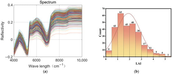
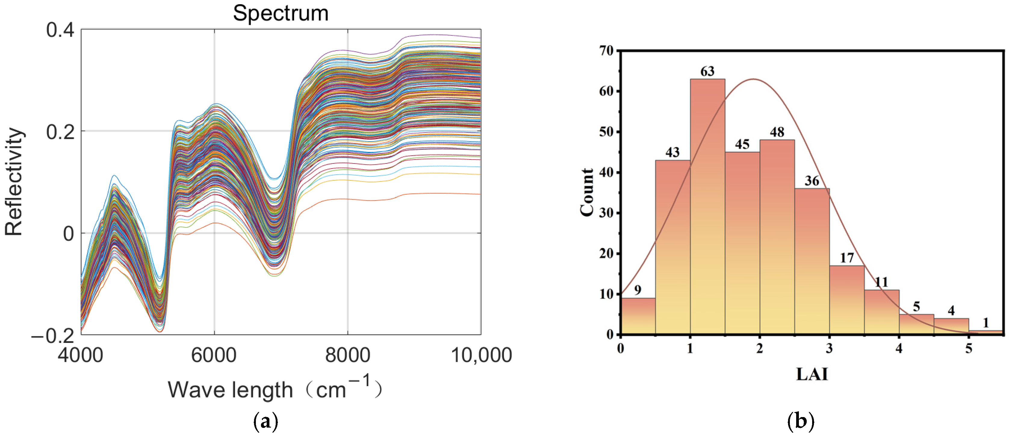
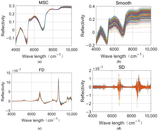
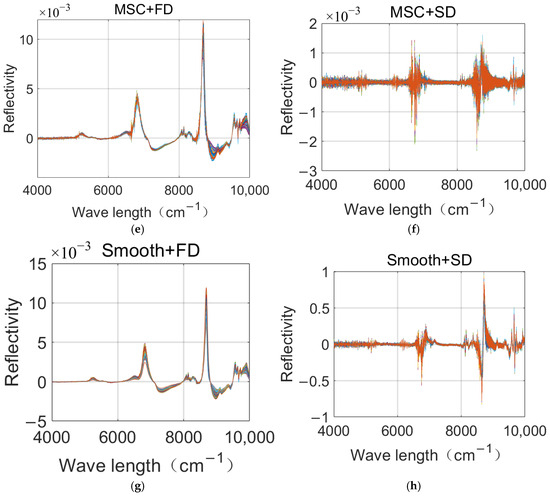
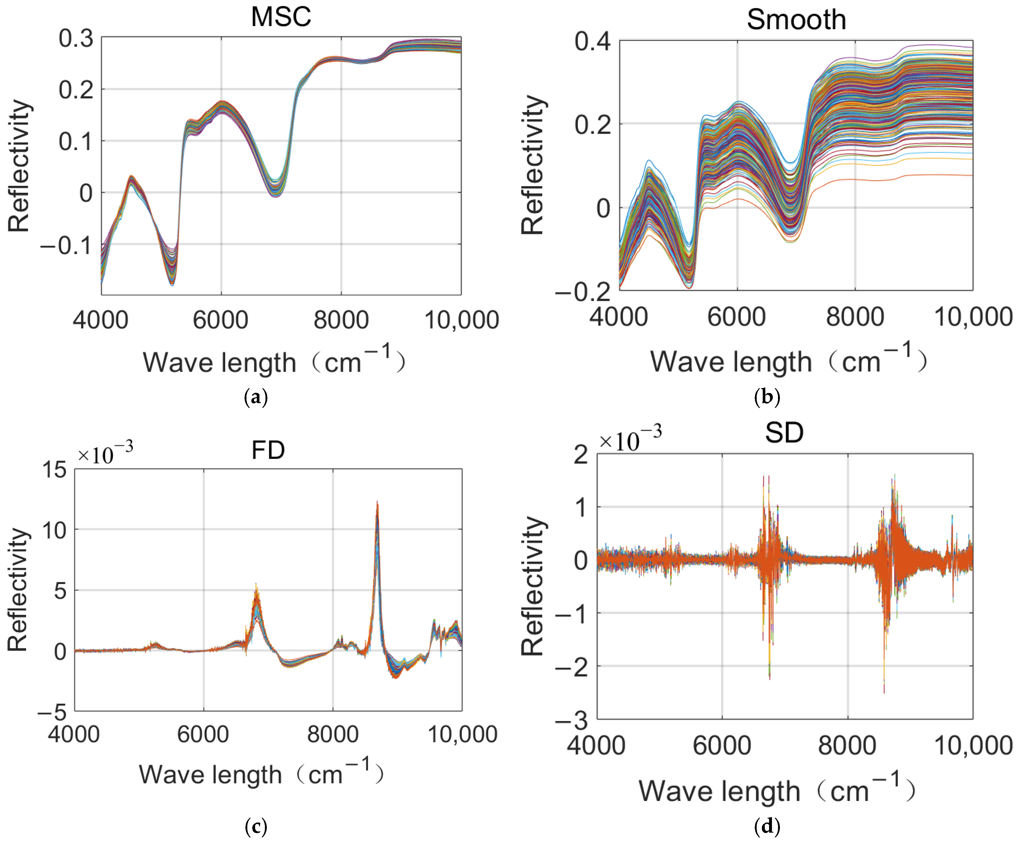
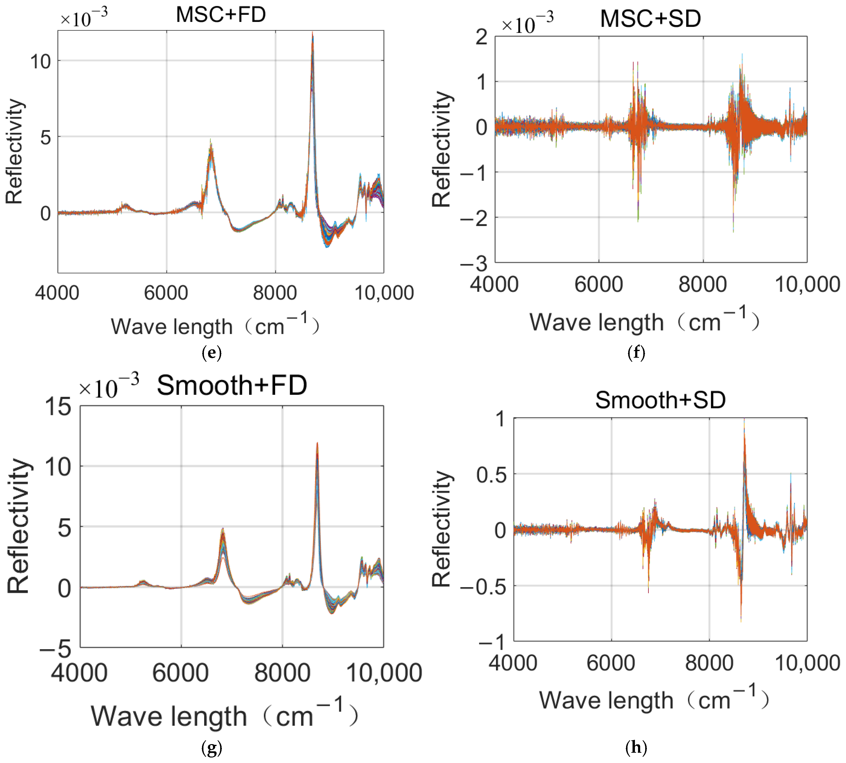
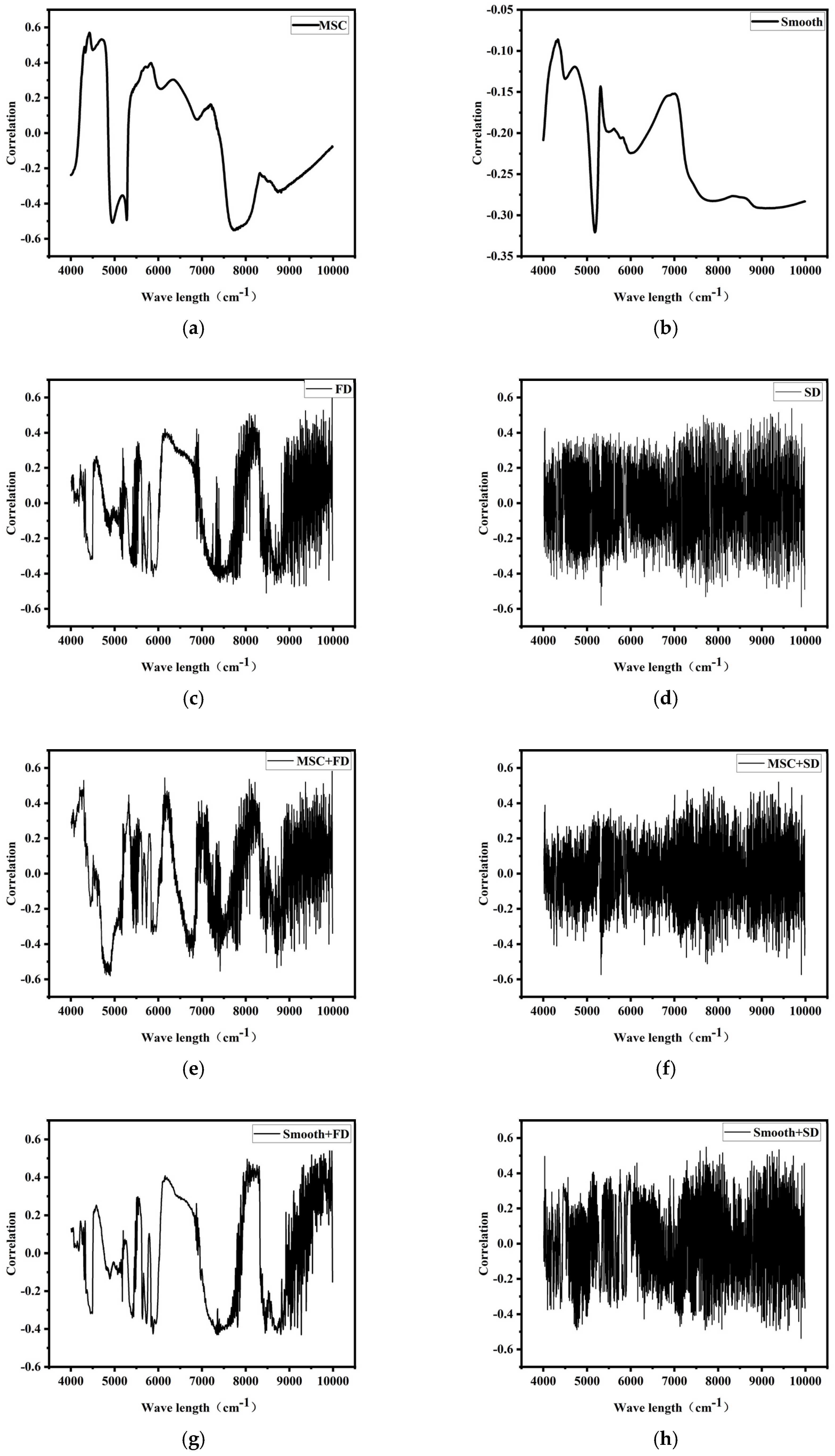
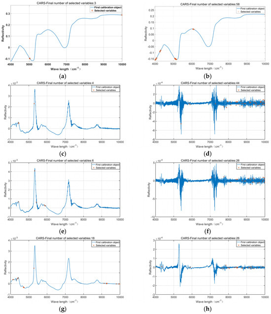
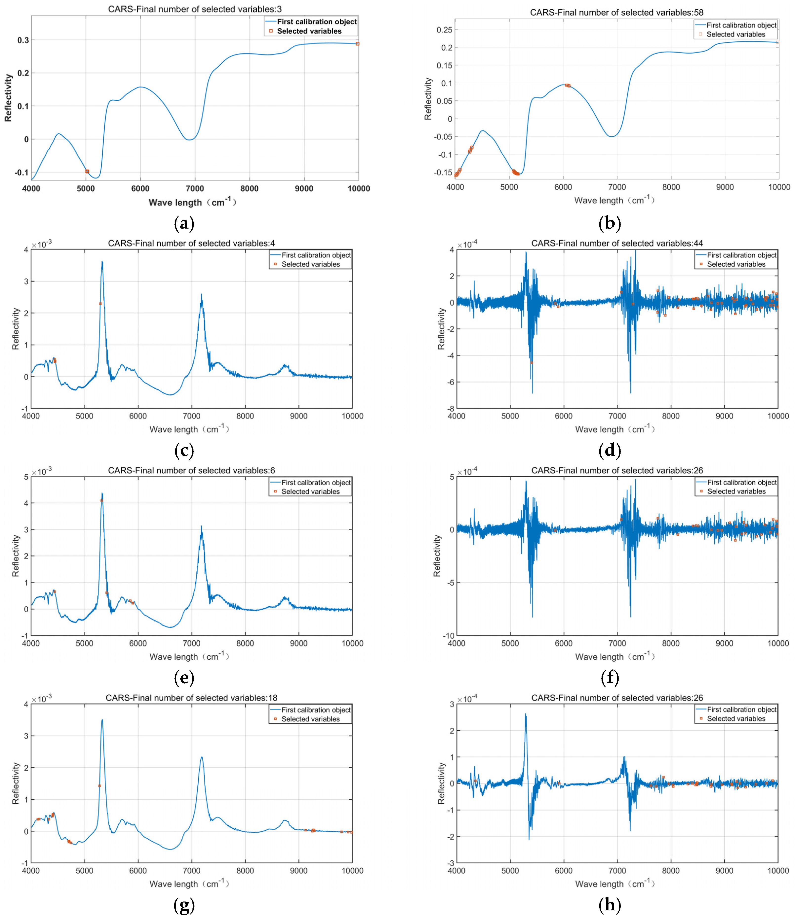
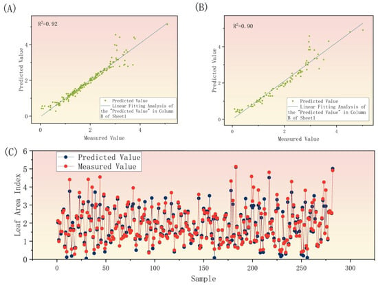
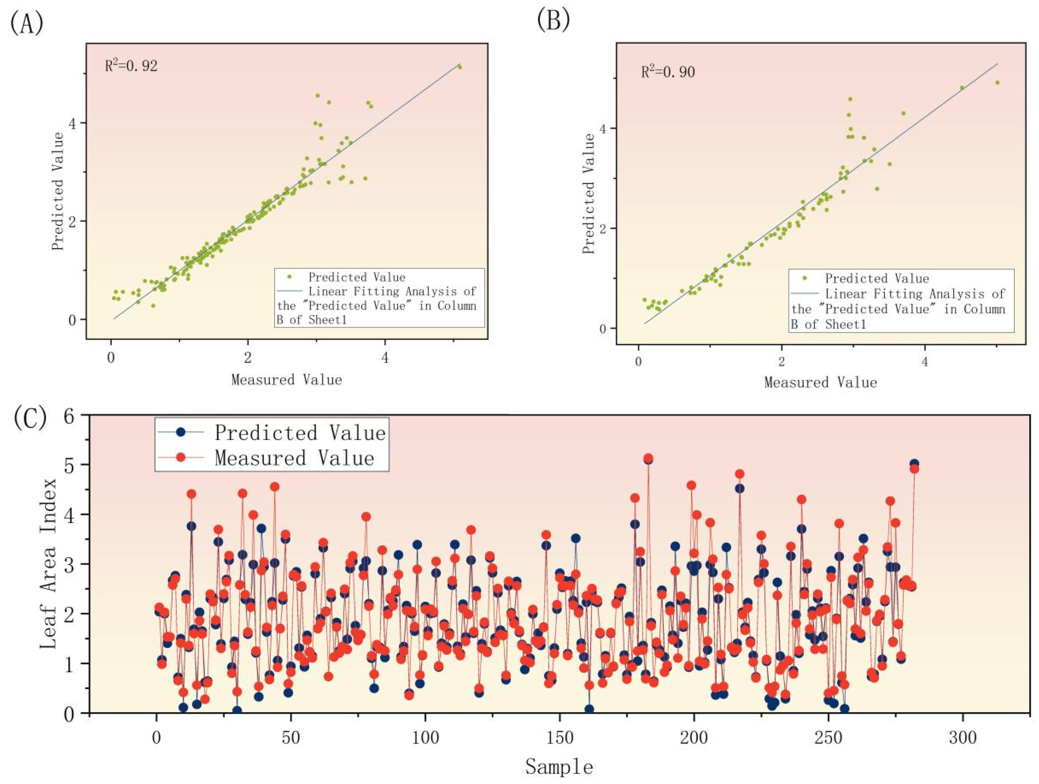

Disclaimer/Publisher’s Note: The statements, opinions and data contained in all publications are solely those of the individual author(s) and contributor(s) and not of MDPI and/or the editor(s). MDPI and/or the editor(s) disclaim responsibility for any injury to people or property resulting from any ideas, methods, instructions or products referred to in the content. |
© 2026 by the authors. Licensee MDPI, Basel, Switzerland. This article is an open access article distributed under the terms and conditions of the Creative Commons Attribution (CC BY) license.