


Highlights
What are the main findings?
- Wall-to-wall aboveground biomass (AGB) and AGB change maps at 10 m and 90 m resolutions reveal spatially heterogeneous hurricane-driven losses (up to ~20% at 10 m and 5% at 90 m) followed by widespread but uneven forest recovery across Puerto Rico.
- Random Forest models integrating FIA plots, LiDAR canopy structure, and multi-temporal satellite data achieved strong performance (r = 0.65–0.83), with 10 m capturing fine-scale disturbance and 90 m improving the model’s goodness of fit.
What are the implications of the main findings?
- Forest carbon losses from extreme hurricanes can be substantial but may be followed by rapid landscape-level recovery, highlighting resilience in secondary tropical forests.
- The transferable machine learning framework provides a practical approach for monitoring forest resilience, informing restoration prioritization, and supporting MRV (Monitoring, Reporting, and Verification) and REDD+ (Reducing Emissions from Deforestation and Forest Degradation) carbon reporting in hurricane-affected regions.
Abstract
Tropical forests are major contributors to the global carbon budget but are affected by disturbances such as hurricanes, which cause extensive yet spatially variable tree damage and mortality. High-resolution maps of forest aboveground biomass (AGB) and its temporal change aid in quantifying disturbance impacts, assessing resilience, and supporting forest management. This study presents wall-to-wall, high-resolution mapping of pre- and post-hurricane AGB and AGB change across Puerto Rico. The maps represent forest AGB measured 0–2 years before and after two major hurricanes (Irma and Maria), as well as longer-term conditions up to four years post-disturbance. AGB was modeled using Random Forest (RF) algorithms that integrated Forest Inventory and Analysis (FIA) plot data with canopy height and cover derived from discrete-return LiDAR, multi-temporal satellite imagery, and additional geospatial predictors. Model performance was evaluated using a 10% holdout dataset. Predicted versus observed regressions yielded, at 10 m and 90 m spatial resolutions, respectively, r = 0.75 and 0.79 with model residual mean standard deviation (RMSD) = 87.7 and 39.2 Mg ha−1 for pre-hurricane AGB, and r = 0.77 and 0.74 with RMSD = 69.7 and 58.1 Mg ha−1 for post-hurricane AGB. AGB change models at 10 m and 90 m resolutions yielded r = 0.58 and 0.73 with RMSD = 17.0 and 18.7 Mg ha−1, respectively. Ten-fold cross-validation produced stronger correlations and reduced RMSD values. Frequency distributions of mapped pixels of forest AGB and AGB change, in comparison with previously published maps and island-wide field-based estimates, indicate that, although hurricane-driven biomass reductions of up to 20% were recorded in field data, patterns consistent with longer-term recovery from historical deforestation are evident within four years after the hurricanes. The 10 m maps capture fine-scale heterogeneity in canopy damage and regrowth, whereas the 90 m maps emphasize broader regional patterns. This integrated framework provides a transferable approach for monitoring forest structure and biomass dynamics in disturbance-prone tropical ecosystems.
1. Introduction
The spatial distribution and magnitude of forest aboveground biomass (AGB) is important for understanding forest productivity and terrestrial carbon cycling from regional to global scales [1,2,3]. These insights are essential for forest management, the development of strategies for carbon offsets and mitigation [4,5], the calibration of biophysical models [6,7,8], and the evaluation of the effects of environmental disturbances on carbon cycling and ecosystem services [9,10,11,12]. Similarly, in regions vulnerable to natural disturbances (e.g., intense forest fires in the Western United States, Amazonian blowdowns, or cyclones in the global tropics), detailed high-resolution biomass mapping is essential for tracking forest carbon dynamics. For instance, Puerto Rico has used general biomass maps to monitor post-hurricane forest recovery, evaluate wildfire risks, and assess the impact of climate change on forest health [13]. After major natural disturbances, detailed and fine-resolution biomass maps have proven vital for assessing forest damage and prioritizing areas for forest restoration and conservation [14].
Traditionally, estimating forest AGB involves detailed, ground-based forest inventories of individual trees and allometric equations [15,16]. Although inventories can yield reliable AGB estimates at local or regional scales, they are not spatially continuous, making it difficult to visualize the spatial distribution of forest biomass. Mapping forest biomass and biomass change can be important for many applications. For example, forest fires in the Caribbean may be more extensive after hurricanes [17], presumably from fuel buildup. As a result, knowing the precise locations of hurricane-related losses in live forest biomass might improve spatially explicit models of wildfire risk. Previous research has used statistical or machine learning methods to link field-estimated biomass, or airborne or spaceborne Light Detection and Ranging (LiDAR) calibrated with field data, with satellite-based optical and/or radar imagery (e.g., [18,19,20,21,22,23]) to generate detailed and spatially continuous biomass maps with neural networks, Random Forests, or other algorithms [24,25,26,27,28]. These spatially continuous depictions of forest biomass hold immense value for local and international stakeholders dedicated to forest conservation and management [29] and are often used to quantify the role of forests in global climate mitigation frameworks [30], including for analyzing disturbance-related land carbon fluxes (e.g., land carbon dynamics following hurricanes). However, biomass maps often lack the detail required for effective forest management due to coarse spatial resolution or limited geographic coverage, or the existing maps are outdated [31,32,33]. National- or continental-scale forest AGB maps with a low spatial resolution may differ from observations at local or regional levels [20,21]. Regression trees were used by [34] to map biomass using Forest Inventory and Analysis (FIA) data from 2001 to 2003 for the conterminous U.S. and Puerto Rico. However, the spatial resolution of 250 m was coarse for the relatively small island of Puerto Rico. In another study, ref. [19] applied the Phenological Gradient Nearest Neighbor (PGNN) method and Cubist regression tree models to map forest AGB at 30 m spatial resolution for Puerto Rico and the U.S. Virgin Islands. Yet, in both cases, the maps may become outdated, given the intense hurricanes that affected Puerto Rico in the year 2017 and that the maps were based on FIA data from the years 2001–2003 (when data were first collected on mainland Puerto Rico under the current FIA sample design).
Hurricanes can have a range of effects, including immediate and delayed tree mortality, alterations in forest structure, and shifts in plant community composition [35,36,37,38]. However, most studies assessing changes in forest biomass in Puerto Rico due to Hurricanes Irma and Maria are limited to specific sites or few field plots. For instance, ref. [39] focused on the Bisley Experimental Watersheds (BEWs) in the Luquillo Experimental Forest and found that tropical forests exhibited a higher resistance to Hurricanes Irma and Maria compared to previous hurricanes, such as Hurricane Hugo in 1989. And ref. [40] analyzed changes in forest structure and composition following major hurricanes in El Verde 3 Plot, emphasizing the dynamics observed with long-term field measurements. Reference [41] also examined the impacts of hurricanes on tropical forest AGB using data from the Luquillo Forest Dynamics Plot. The available larger-scale studies only emphasize hurricane-related drivers of forest canopy changes immediately after the hurricanes [38,42,43,44], or hurricane-related drivers of tree mortality [36,38].
Here, to extend the temporal scope of analysis across mainland Puerto Rico, this study develops wall-to-wall maps of forest aboveground biomass (AGB) and associated changes before and after the 2017 hurricanes. The primary aim is to advance the spatial mapping of AGB and AGB change by integrating forest inventory data with high-resolution geospatial datasets at two spatial resolutions. We generate spatially explicit AGB maps representing conditions during the two years preceding and the two years following the hurricanes and AGB change over a longer post-disturbance period of up to four years.
Using machine learning techniques, we integrate FIA plot data with predictor variables derived from discrete-return LiDAR (forest height and canopy cover), satellite image composites, climate data, and topographic variables from fine-resolution digital elevation models.
The specific objectives are to: (1) produce and comparatively evaluate wall-to-wall AGB and AGB change maps at 10 m and 90 m resolutions, assessing how dual-resolution analysis captures contrasting aspects of fine-scale hurricane disturbance heterogeneity and landscape-scale recovery patterns; (2) evaluate the suitability of small FIA subplot data (168 m2) as training samples for fine-resolution (10 m) tropical AGB mapping in a topographically complex island landscape; and (3) identify the relative importance of multi-source predictors (e.g., LiDAR, multi-temporal imagery, climate, and topography) and assess their consistency with known drivers of hurricane-related tree mortality.
The framework developed in this study is transferable beyond Puerto Rico and can support spatially explicit biomass monitoring and disturbance assessment in other forested regions.
2. Materials and Methods
2.1. Study Area
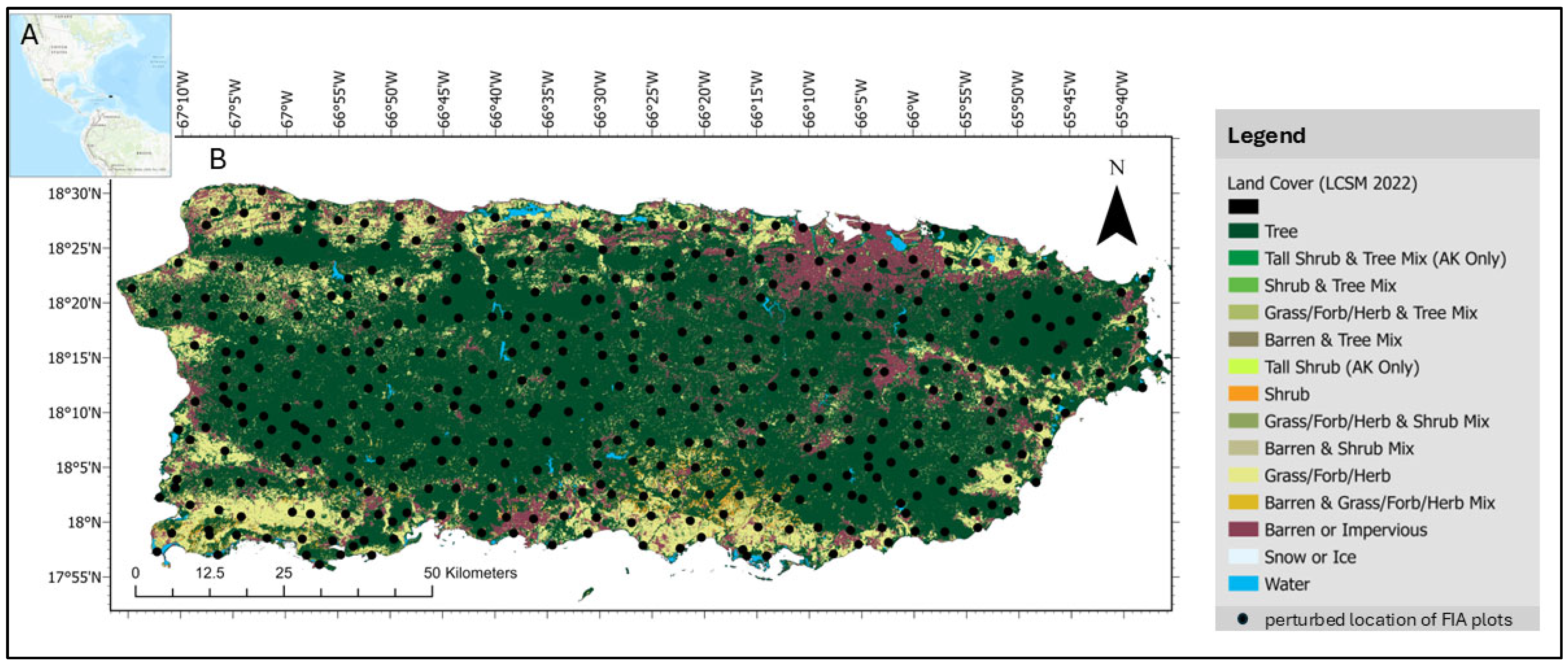
This study focuses on mainland Puerto Rico (Figure 1). The island is ~52% forested, including tropical dry, moist, wet, and cloud forest [45], with a varied geology over a relatively small area (8870 km2). The island experiences a significant range in annual rainfall, from 800 to 4500 mm per year [46].
Puerto Rico is subject to tropical cyclones from June through November, with peak activity in August and September [47]. Hurricane frequency in Puerto Rico is among the highest in North America, with major stand-damaging hurricanes occurring about every 50–60 years [48]. From 1900 to 2017, 33 named cyclones have impacted Puerto Rico (i.e., passed within 138 km of its coastline). Of these, 14 reached major hurricane intensity, including Hugo in the year 1989, Georges in 1998 and Irma and Maria in 2017 [49].
Figure 1.
The land cover of mainland Puerto Rico and the perturbed location of FIA plots. (A): Puerto Rico in relation to North and South America; (B): land cover map [50] of mainland Puerto Rico, dots represent perturbed location of FIA plots; (The FIA plot design and topography are shown in Figures S1 and S2.
2.2. Field and Auxiliary Data
As described below, field data came from United States Department of Agriculture Forest Service (USFS) Forest Inventory and Analysis (FIA) data. Predictor variables (Table S1) included multispectral satellite imagery, topographic variables from a digital elevation model (DEM), long-term climate maps, canopy height and cover mapped from discrete LiDAR, maps of geological substrates, and a forest age map.
2.2.1. Forest Inventory and Analysis (FIA) Data
We used the FIA data as ground measurements of Puerto Rico’s mainland forest characteristics, including tree size. Each FIA measurement plot consists of four subplots (Figure 1C and Figure S1), with the cumulative area of these subplots totaling 672 m2 [51]. FIA samples trees ≥ 12.7 cm dbh within the four 167 m2 plots, and trees 2.5 to 12.6 cm dbh within 54 m2 microplots within each of the four subplots [52]. For our analysis, subplots were treated both as nested within plots and as independent observation units, depending on the model scale. At the subplot scale (10 m), each subplot was considered separately to capture fine-scale variability. At the plot scale (90 m), biomass was aggregated across the four subplots to represent the entire plot. This dual approach ensured that the plot design was consistently matched to the resolution of the predictive models. Trees are surveyed if any portion of a plot has 10% tree canopy cover or had 10% tree cover and is likely to be reforested. A subset of one-third of the plots shown in Figure 1 are sampled in each year of a three-year measurement cycle, and two years pass between measurement cycles.
Each inventory cycle for mainland Puerto Rico consists of three 1-year subcycles that survey one-third of the plots every five years. Two of the small outlying islands of Puerto Rico are surveyed in the fourth year. Consequently, for the AGB maps, pre-hurricane (pre-H) data included data from 2016 (pre-H subcycle 1) and January to September 2017 (pre-H, most of subcycle 2). Data from October 2017 through 2018 represented post-H, mainly subcycle 3. For the AGB change maps, we used the differences between plots measured over the times October–December 2012 to October–December 2017, 2013 to 2018, and 2016 to 2021. Mainland Puerto Rico plots were not scheduled to be surveyed in the years 2014, 2015, 2019, or 2020. We included only fully forested plots and subplots (analyses done at both scales) based on their field-recorded condition and as identified on a 2022 land cover map from [50], resulting in 653 pre-H and 450 post-H subplots and 131 pre-H and 207 post-H plots; 349 subplots and 138 plots were used for AGB change mapping.
We note that, based on the above FIA data, which identify tree mortality agents, about 79% of the basal area of tree mortality of the plots surveyed from after the 2017 hurricanes to the year 2021 was due either to those storms (78%) or to fires on hurricane-damaged plots after those storms (1%). Other tree mortality was recorded as being due to vegetation competition (20%) or disease (1%).
2.2.2. Remote Sensing Data
We integrated the Normalized Difference Vegetation Index (NDVI) and the Normalized Difference Infrared Index (NDII) from Landsat image composites centered on the years corresponding to pre- and post-hurricane periods (sourced from [19,36,53,54]) to indicate forest greenness and wetness, respectively [55]. The NDII contrasts the Near-Infrared (NIR) and Shortwave Infrared (SWIR) wavelengths and is sensitive to forest water content, which can be representative of forest health and structural attributes like canopy closure [55].
Also known as the Normalized Difference Infrared Index, NDII can effectively detect plant water stress due to its sensitivity to SWIR reflectance, which is inversely related to leaf water content. Vegetation indices with contrasting NIR and SWIR bands are also sensitive to forest structure, disturbance and successional stage, including in Caribbean forests [17,36], perhaps because they are sensitive to the overall water content of forest canopies [55].
The satellite image composites consisted of (1) multiband imagery, in which image composites were produced on a per-band basis and vegetation indices were then calculated from the multiband composited imagery, and (2) phenology metrics extracted with threshold-based methods.
The historical multiband Landsat Multispectral Scanner image composites circa 1980 and 1985 and the Landsat Thematic Mapper (TM) composite circa 1990 [19,56] are mosaics of the clear parts of many single-date images that were radiometrically normalized to one early dry season base scene with regression trees and histogram matching following the methods from [57]. These image inputs are available for download [56].
The Landsat composites circa the year 2000 and later [54] composited the per-band median reflectance values for the three earliest and three latest of those pixel observations flagged as unlikely to be cloudy during the compositing time period [58]. The images are composites of Enhanced Thematic Mapper (ETM+) or Operation Land Imager (OLI) scenes.
The Landsat phenology metrics [36,53] were developed using the methods from [59]. The Enhanced Vegetation Index (EVI) was calculated from atmospherically corrected imagery for all Landsat ETM+ and OLI images from the years 2010–2014. Pixels flagged as noncloudy were ordered as though from one year, then phenology metrics were calculated.
Sentinel-2 imagery [60], assigned to the output composite image on a per-band basis, provides the pixel value of the 25th percentile of those pixels flagged as least likely to be cloudy over the compositing time period. These composites provide a cloud-free, global mosaic derived from Sentinel-2 imagery collected between January 2017 and December 2018. This composite was generated using the Sentinel-2 archive available through Google Earth Engine and consists of a pixel-level mosaic incorporating four spectral bands, Blue (B2), Green (B3), Red (B4), and Near-Infrared (NIR, B8), each at a spatial resolution of 10 m [60]. The Red (B4) and Near-Infrared (NIR, B8) spectral bands of the Sentinel-2 Global Pixel-Based Image Composite from Level-1C data [60], along with the calculated NDVI, were used as predictors in the modeling process.
Canopy height and cover with a 1 m spatial resolution from discrete return LiDAR from the years 2016 and 2018 were sourced from [61].
2.2.3. Forest Age Map
We included a forest age map of Puerto Rico. The stand age classes range up to the class of 50–64+ years, representing well-conserved evergreen forests in areas like El Yunque National Forest/Luquillo Experimental Forest and the dry forests of the Guánica Commonwealth Forest. New-growth forests aged 1 to 5 years occur across the southwest. The forest age map [53,62] combined land cover maps developed with Landsat imagery, with a pixel size of 30 m from circa 1990 and 2000, with air photo-based land cover maps from 1977 and 1951, with approximate scales of 200 m and 1200 m, respectively. Given the coarse resolution of the map from 1951, the age map had a relatively coarse spatial resolution, which likely added uncertainty to our analyses.
2.2.4. Topographic Variables
We used elevation, slope, slope position, aspect classes, and overall, profile, and plan curvatures from a 10 m digital elevation model (DEM) [63]. The boundaries of the island came from Puerto Rico Shoreline 2019 data from [64]. The 2022 land cover map from [50] was used to differentiate forested from non-forest areas of raster images.
2.2.5. Climate Variables
The climate variables considered in the models, including temperature and precipitation, came from Daymet (Daily surface Weather and Climatological Summaries) (1979–2019; [65]) and PRISM (Parameter-elevation Regressions on Independent Slopes Model) data (1963–1995; [66]). For subplot-scale and plot-scale analyses, all pixels were resampled to a 10 m and 90 m spatial resolution through nearest neighbor resampling. The PRISM climate maps [66] were developed at a spatial resolution of 15 s (~450 m). Daymet climate maps have a spatial resolution of 1 km. The coarse spatial resolutions of the climate data relative to the remote sensing data likely added uncertainty to the biomass mapping models.
2.2.6. Regional and Global AGB Maps for Comparison
Besides reserving 10% of the plot data for model validation, we compared the frequency distributions of the AGB maps with a regional-scale biomass map, representing the mainland Puerto Rico forest biomass circa the years 2001–2003 (28.5 m resolution), which was from [19] (hereafter H-2018). In addition, we compared the pre-H and post-H AGB maps to two global biomass maps from the European Space Agency (ESA) Climate Change Initiative (CCI), representing forest biomass for the years 2017 and 2018 (hereafter ESA-2017 and ESA-2018) [67]. The ESA CCI data provide estimates of forest AGB at a 100 m spatial resolution derived by combining Earth observation data from various sources [67]. Section 2.3.3, Model Validation, describes our approach for these comparisons. We note that the ESA-2017 map may not entirely represent pre-hurricane conditions, as it is possible that the model for the map included some reference AGB observations from after the hurricanes in the year 2017.
2.3. Biomass Computation and Random Forest Modeling
To create a training dataset for RF modeling, we combined FIA plot data with LiDAR-extracted tree percent canopy cover (%) and height (m), image bands, indices from remotely sensed image composites, and the other predictor variables. The workflow summary has four main steps (Figure 2). First, we estimated biomass from FIA measurements at both subplot and plot levels by applying the improved allometric equation for tropical tree biomass from [68]. This step provided a baseline for model training and validation. Next, the geospatial data were processed to match the spatial resolution and extent of the FIA subplot/plot data. Then, we developed predictive models with the Random Forest (RF) machine learning algorithm, which was used to generate continuous biomass maps across the study area. Biomass maps were validated by comparing model predictions and uncertainties with the randomly selected 10% subset of the FIA subplot or plot-level estimates and existing regional and global biomass maps.
Figure 2.
Workflow for generating aboveground biomass (AGB) maps and biomass change (ΔAGB) maps for Puerto Rico. FIA plot and subplot data were used as response variables, and geospatial data (canopy height and cover from discrete LiDAR, satellite imagery, climate, topography, etc.) were used as predictors for Random Forest mapping models. Outputs included pre-hurricane AGB maps, post-hurricane AGB maps, and ΔAGB maps (biomass change derived from FIA plot-level differences), illustrating the parallel modeling approach applied to each product.
Note that we filled the gaps in the LiDAR-based canopy height data from the year 2016 with the canopy height maps from [19]. The height map described in that publication was created using the mean height of dominant and codominant trees from inventory data dated from 2001 to 2003 as the mapping model response variable. Predictor variables in the models included multispectral satellite imagery and a canopy height model derived from coarse-resolution discrete return lidar (~3 m shot spacing) developed with the methods from [63] and other geospatial data. To fill the gaps in LiDAR-based canopy cover, we used the USFS National Land Cover Database Tree Canopy Cover Datasets [64].
2.3.1. Biomass Computation from Field Data
We used the BIOMASS package in R4.3.3 [69] to apply the allometric model from [68], estimating tree AGB using the following equation:
where WD is the wood density (g/cm3), H is the canopy height (m), D is the tree diameter (cm), and AGB is the aboveground biomass (kg). This equation is known for its lower bias in AGB estimates compared to other allometric equations, particularly when trunk diameter, total tree height, and wood-specific gravity are provided. This equation is robust, showing no detectable effect of regional or environmental factors [68]. WD measurements were sourced from the comprehensive global wood density database [70,71] and wood density measurements from [53]. Genus and family level means were used where data were missing for species. Such occurrences comprised 24% of species at the genus level and 5% of species at the family level. Next, the AGB of individual trees was summed at the microplot or subplot level and divided by the total microplot or subplot forested area.
AGB = 0.0673 × (WD × H × D2)0.976
2.3.2. Spatial Resolution for Random Forest Modeling
We mapped forest biomass at 10 m and 90 m resolutions because those resolutions have potential advantages given the available field and remote sensing data. We tested the 10 m resolution because, when field plots fill the pixel sizes of remote sensing data, bias in AGB mapping models is reduced [72]. The FIA subplots (168 m2) fill 10 m pixels, and the Sentinel-2 imagery, the digital elevation model (DEM), the SPOT pan band from 1995, and the forest canopy height and cover data that we use have 10 m or smaller cells. In addition, topographic variation is important to consider when defining the scale for forest AGB mapping [72]. Where rugged karst topography occurs in Puerto Rico, tree communities and wind exposure can vary at scales as fine as 10 m or less. Tree mortality and resistance to hurricanes also varies among the tree communities there [36]. Furthermore, 10 m cells would more likely capture AGB change related to stem breakage or the mortality of single trees. As for the 90 m resolution, we tested it for three main reasons: (1) mapping models of forest AGB that rely on FIA data can be more accurate at the plot rather than the subplot scale, at least when comparing 90 m with 30 m pixel sizes [73]; (2) 90 m aligns well with the 3-by-3 window of the 30 m pixels composing much of the contemporary and historical Landsat satellite imagery; and (3) plot-level data should capture more large trees.
Small forest plots are not always optimal for mapping forest AGB, but FIA data, despite a total size of 0.067 ha, has advantages for our study area. Some researchers suggest that the plots calibrating forest AGB mapping models should span at least 0.1 ha for temperate and boreal forests and 0.25 ha for tropical forests, depending on the large tree size [74]. But existing networks with field plots this large represent neither the range of secondary tropical forest disturbance histories nor the range of other conditions affecting forest AGB. Dry and montane tropical forests, and the ranges of edaphic conditions and geological substrates underlying tropical forests, are not well represented in these networks [75]. In contrast, National Forest Inventory (NFI) data with small field plots may be the only field data covering the range of forest conditions across a region [36]. The FIA plots are the only field data that represent the range of Puerto Rico’s forests. They include dry, humid, and montane tropical forests of different ages, disturbance histories, and soils, including edaphically dry to saturated soils and those over serpentine geology. Moreover, mitigating the challenge of small field plots including large trees is that, in Puerto Rico, small trees (dbh < 12.7 cm) can represent a large component, up to 50%, of forest AGB [76]. Finally, the median canopy diameter of Puerto Rico trees with a dbh ≥ 12.7 cm is 12 m (based on the data described in [16]), which is close to the 10 m typical canopy diameter of large temperate forest trees that [74] used to recommend the 0.1 ha plot size minimum.
We note that the FIA subplot (radius 7.3 m, area ~168 m2) is geometrically larger than a single 10 m pixel (100 m2), extending approximately 3.6 m beyond the pixel boundary. In most of Puerto Rico’s forests, where canopy structure changes gradually, this mismatch is unlikely to cause systematic bias because adjacent pixels tend to have similar AGB values, and only the subplot center coordinate is used for pixel matching. In high-contrast karst landscapes, where tree communities can shift significantly at scales of 10 m or less, the subplot AGB may incorporate signals from neighboring pixels; this represents a source of training noise in those areas, which we note as a component of the spatial resolution mismatch uncertainty discussed in Section 4.5.
Evaluating both the 10 m and 90 m scales enables us to assess the trade-offs between detail and model accuracy, while ensuring that biomass predictions are ecologically and statistically consistent with the FIA measurement framework.
Resampling Landsat pixels to 10 m with a nearest-neighbor approach meant that each 30 m Landsat pixel was subdivided into nine identical 10 m pixels. This resampling is unlikely to have influenced the spatial autocorrelation in pixels used for model training, because only the center of the resampled Landsat pixel is used for model training and testing. It might add more spatial autocorrelation to output biomass maps than other resampling methods. We selected nearest-neighbor resampling, however, to preserve the original spectral information.
2.3.3. Model Validation
The RF algorithm is a powerful, nonparametric, ensemble-based machine learning technique that reduces overfitting by aggregating predictions from a large number of unpruned regression trees [77]. Each tree is built using a bootstrap sample of the training data, and at each split a random subset of predictor variables is considered. This stochastic approach enhances model generalization, reduces variance, and makes RF resilient to noisy data and overfitting. A key strength of RF is its ability to handle both categorical and continuous variables, while also demonstrating robustness to multicollinearity, noise, and high-dimensional datasets [78]. Similarity among observations is quantified by their co-occurrence in terminal nodes across all trees, with proximity defined as one minus the proportion of trees in which a target and reference observation share the same terminal node [77].
Compared to traditional regression tree models, RF shows a superior predictive performance and has been widely adopted in remote sensing and forest inventory applications, particularly for estimating aboveground biomass and mapping forest structure and carbon stocks [79,80,81]. In this study, RF models were implemented using the ModelMap 3.4.0.8 package [82], which is specifically designed for ecological modeling. All RF models were run with ntree = 500 trees and mtry = 6 for pre-H subplot, pre-H plot, post-H subplot, and post-H plot modeling, and with mtry = 3 for AGB change modeling. Out-of-bag error was plotted as a function of tree count for each model to verify convergence; in all cases, error stabilized before 200 trees, confirming that 500 trees was sufficient.
For model validation, we randomly reserved 10% of the FIA field observations as an independent holdout dataset that was not used during model training, providing an unbiased test of predictive performance, as is common in remote sensing studies (e.g., [73]). To assess model stability with a larger dataset, we also conducted a 10-fold cross-validation in which the entire dataset was partitioned into ten equal subsets, with each subset used once for testing while the remaining nine subsets were used for training. The 10% holdout results are presented in the main text, and the cross-validation results are presented in Supplementary Figure S1. The correlation coefficient (r) and the root mean square deviation (RMSD) between model predicted values and observations are presented to assess model fit and overall model error. RMSD is the quadratic mean of the differences between the observed and predicted values.
To avoid ambiguity, we distinguish between model error and map uncertainty. Model error refers to the overall predictive performance evaluated against validation datasets, reported here as correlation (r), root mean square deviation (RMSD), and related statistics. In contrast, map uncertainty refers to pixel- or local-level variability in predictions, which we assessed using the coefficient of variation across RF trees. Throughout this manuscript, we use “error” when describing model performance against validation data and “uncertainty” when referring to the spatial heterogeneity in prediction confidence across the biomass maps.
In addition to reporting correlation coefficients (r) and root mean square deviation (RMSD), we incorporated two additional metrics to provide a more comprehensive evaluation of model predictive performance. First, we calculated relative RMSD (rRMSD), defined as RMSD divided by the mean observed AGB × 100%. This metric contextualizes absolute error relative to the magnitude of observed biomass and enables a comparison across resolutions and model configurations. Second, we computed the coefficient of determination with respect to the 1:1 line (R21:1), which quantifies the degree to which predictions align with perfect agreement rather than the fitted regression line. R21:1 avoids the inflation of perceived performance when model predictions systematically deviate from the 1:1 relationship, such as underestimation at high AGB or overestimation at low AGB. These metrics were computed for all plot- and subplot-level models, including pre-hurricane, post-hurricane, and AGB change models.
To visualize model performance and assess spatial variability in AGB map uncertainty, we computed the coefficient of variation in AGB as the standard deviation (SD) divided by the mean for every RF tree [82,83]. Additionally, we compared the AGB maps from this study to those from (1) AGB maps using FIA data from the years 2001–2003 (H-2018) and (2) AGB maps from the ESA CCI data (downloaded from [67]) for the years 2017 (ESA-2017) and 2018 (ESA-2018), approximately corresponding to AGB before and after the late-2017 hurricanes, respectively. The comparisons with the ESA CCI maps were pixel-level comparisons, and the Fuzzy Numerical Index (FNI) was calculated to quantify the overlap between two fuzzy sets relative to their combined extent. FNI provides a normalized measure (ranging from 0 to 1) of the similarity between two spatial datasets based on fuzzy logic principles that handle the uncertainty and partial truth inherent in spatial data [20]. This measure is robust against small variations in spatial datasets and is sensitive to the overall pattern and distribution of values within them [73].
In addition, we evaluated the strength of the relationships between our AGB maps and global biomass products to further evaluate the Puerto Rico maps. For this comparison, we first harmonized all raster layers to a 90 m spatial resolution with nearest-neighbor resampling. To minimize the influence of spatial autocorrelation on these comparisons, we then randomly sampled 1000 pixels from the pre-hurricane (pre-H) map and extracted corresponding values from the ESA, H-2018 and our post-H maps developed at the plot level. For each pairwise comparison (pre-H vs. ESA-2017, pre-H vs. H-2018 (H-2018 represents conditions circa the years 2001–2003) and post-H vs. ESA-2018), we calculated Pearson’s correlation coefficient, root mean square deviation (RMSD), and bias (mean difference). Additionally, we performed paired t-tests and Wilcoxon signed-rank tests to assess whether mean differences were statistically significant.
2.3.4. Spatial Mapping of Biomass Change
As illustrated in the workflow (Figure 2), we generated AGB change maps with the same RF modeling process as the pre- and post-hurricane AGB maps, with the FIA plot-level differences (post–pre) serving as the response variable. AGB change is measured in megagrams per hectare (Mg/ha), with positive values indicating stand AGB increase and negative values indicating AGB loss. To validate the maps, we calculated r and RMSD between predicted vs. observed ΔAGB for a 10% holdout sample for both the 10 m and 90 m spatial resolutions.
We also plotted smoothed density estimates [84] to illustrate the frequency distributions of pixels in the RF-modeled AGB change maps together with the frequency distribution of pixels resulting from subtracting the ESA CCI global biomass maps from the year before vs. the year after the hurricanes (i.e., ESA-2018 minus ESA-2017).
As mentioned, our main objective is to investigate the mapping of AGB changes from the years before to those after the 2017 hurricanes. Toward that goal, we also analyzed whether AGB change mapped at 10 m or 90 m was significantly associated with the distance from the eye of Hurricane Maria because it passed directly over Puerto Rico (The best track of the hurricane eye was downloaded from [46]). Distance to the hurricane track explained some variability in hurricane-related tree mortality [38]. It is also independent of the AGB change maps because, unlike topographic and climate variables, it was not used as a predictor variable for mapping AGB change.
Finally, we discuss whether the landscape variables important to mapping AGB change are consistent with the landscape variables associated with hurricane-related tree mortality.
3. Results
3.1. Subplot- and Plot-Level Biomass
From the field data, AGB at the subplot scale (10 m) across Puerto Rico revealed a high variability (Figure 3), with maximum values reaching 423 Mg/ha pre-H and 344 Mg/ha post-H. The mean AGB values were 118 Mg/ha before and 110 Mg/ha after the hurricanes, with pre-H and post-H standard deviations (SD) of 102 and 95.3 Mg/ha, respectively. The median pre-H and post-H AGB were 90.9 and 86.4 Mg/ha, respectively. At the coarser plot scale, the maximum AGB values were smaller than at the subplot scale, being 314 Mg/ha pre-H and 290 Mg/ha post-H. The mean pre-H and post-H AGB were 91.2 Mg/ha and 86.3 Mg/ha, respectively. The variability of the plot-level estimates (SD 64 Mg/ha pre-H and 67 Mg/ha post-H) was less than the SD of estimates at the subplot scale, highlighting the fine-scale heterogeneity of forest biomass.
Figure 3.
Histograms of AGB (Mg/ha) from FIA observations before (Pre) and after (Post) hurricanes at two spatial scales. (a) Subplot- and (b) plot-scale data. Transparent color-coded bars (blue = pre, orange = post) show the distribution of AGB, with dashed lines indicating the mean and dotted lines indicating the median. Summary statistics (mean, median, and standard deviation) are shown in color-coded boxes adjacent to the legend for clarity.
3.2. Random Forest Models of AGB
To clarify the extent and influence of LiDAR data gaps on our AGB modeling, we quantified the spatial coverage of missing canopy height pixels in both LiDAR acquisitions. Across the forested region, the 2016 LiDAR canopy height layer contained 4.08% missing pixels, while the 2018 post-hurricane LiDAR layer contained 4.41% missing pixels. These gaps were restricted to small, spatially clustered areas associated with incomplete flight-line overlap and localized data quality issues. These gaps were spatially limited and occurred primarily along flight-line edges and areas with incomplete LiDAR sampling. Because canopy height is one of the most influential predictors in the Random Forest models, these gap areas were filled using auxiliary height products to ensure full spatial coverage. The relatively small extent of these gaps indicates that gap-filling affects only a minor portion of the landscape; however, we note that predictions within these gap-filled regions may exhibit higher localized uncertainty due to the reliance on secondary data sources. We now explicitly document these gap extents and acknowledge their potential implications for model precision.
Model performance was evaluated with an independent 10% holdout dataset (Figure 4) and a 10-fold cross-validation (Figure S3). With both the independent holdout and the cross-validation, the predicted AGB was more strongly related to the observed AGB at the plot (90 m) scale than at the subplot (10 m) scale. As expected, cross-validation yielded slightly higher correlations and lower RMSD values for forest AGB than the independent holdout (e.g., subplot scale r ≈ 0.75–0.77 vs. 0.65–0.70; plot scale: r ≈ 0.80–0.83 vs. 0.73–0.74). The independent holdout provides a conservative estimate of RF model generalization. Cross-validation demonstrates the full predictive capacity of the RF models, as it is trained on all available data.
Figure 4.
Observed versus predicted AGB from RF models, based on validation with an independent 10% holdout of field measurements, at subplot (10 m) and plot (90 m) scales before (pre-H) and after (post-H) the 2017 hurricanes. Panels show (a) pre-H at subplots, (b) post-H at subplots, (c) pre-H at plots, and (d) post-H at plots. The 1:1 line indicates perfect agreement. Each panel includes performance metrics: root mean square deviation (RMSD), Pearson’s correlation coefficient (r) with p-value, and Spearman’s rank correlation coefficient (ρ) with p-value.
Model performance metrics with an independent 10% holdout dataset, including r, RMSD, rRMSD, and R21:1, are summarized in Table 1. Across models, plot-level predictions exhibited a stronger agreement with observations than subplot-level predictions, and pre-hurricane models generally outperformed post-hurricane models. For AGB change models, rRMSD values were large in magnitude due to the small mean observed AGB change, which amplifies relative error; nevertheless, the RMSD and R21:1 values accurately reflect the degree of predictive uncertainty. R21:1 values were consistently lower than r2, indicating a systematic divergence from the 1:1 line and highlighting the importance of including this metric in model evaluation. These results underscore the challenges of capturing fine-scale AGB variability and hurricane-induced changes, while also demonstrating the value of multiple error and agreement metrics for transparent performance assessment.
Table 1.
Model performance summary.
At the subplot scale before the hurricane, pre-hurricane canopy height and NDII were the most important RF model variables (Figure S4, summarized in Table 2). NDVI, temperature seasonality, precipitation of the driest month, aspect class and the 1995 pan band also had a high importance. After the hurricane, pre-hurricane canopy height and NDII remained dominant; however, post-hurricane variables, including canopy height and NDII, also had a high importance. Historical spectral information, particularly the pan band from 1995, and precipitation increased in importance. At the plot scale pre-H, canopy height, canopy cover, and NDII were the primary predictors, with historical spectral factors contributing more substantially at this coarser resolution, including the 1995 band and the red band from 1980. Following the hurricane, pre- and post-hurricane canopy cover and height and NDII continued to be the dominant variables, while Sentinel-2 NDVI and precipitation of the driest quarter (BIO17) became more influential (Table 2).
Table 2.
Top five dominant predictors of AGB across model types and scales.
These results suggest that historical spectral information and climate information were important in addition to contemporary spectral information, and that the LiDARderived variables and NDII were usually the most highly ranked and were consistently in the top three most important variables. In addition, while pre- and post-hurricane LiDAR variables were highly ranked in post-hurricane AGB models, the canopy height in 2016 was typically more important than post-hurricane canopy height, which we discuss later.
3.3. Biomass Maps and Uncertainty
By generating the AGB map at 10 m and 90 m resolution (Figure 5), we found similar spatial patterns across the study area, with the finer-scale RF maps (10 m) depicting more biomass variation. The spatial distribution of biomass also aligns with the LiDAR-derived canopy cover map (Figure S5).
Figure 5.
RF-modeled maps of biomass of tropical forests in mainland Puerto Rico, with associated error represented as the coefficient of variation. (a) Pre-H at 10 m spatial resolution; (b) post-H at 10 m spatial resolution; (c) pre-H at 90 m spatial resolution; (d) post-H at 90 m spatial resolution; (e) pre-H coefficient of variation at 10 m spatial resolution; (f) post-H coefficient of variation at 10 m spatial resolution; (g) pre-H coefficient of variation at 90 m spatial resolution; (h) post-H coefficient of variation at 90 m spatial resolution.
At the subplot (10 m) resolution, RF-estimated AGB values ranged from 18.2 to 405 Mg/ha pre-H (mean = 116 Mg/ha, SD = 42) and from 17.9 to 325 Mg/ha post-H (mean = 106 Mg/ha, SD = 35.6). At the aggregated plot (90 m) scale, AGB estimates ranged from 14.7 to 213 Mg/ha pre-disturbance (mean = 87.9 Mg/ha, SD = 34.2) and from 14.1 to 206 Mg/ha post-disturbance (mean = 82.8 Mg/ha, SD = 32.7). In line with the larger maximum field-surveyed AGB at the subplot level, the maximum predicted AGB, which as mentioned is often underestimated in AGB mapping models, was larger at 10 m than at 90 m. At the same time, model performance improved notably at the plot level, where spatial aggregation reduced the variability in AGB, which enhanced the predictive stability.
This dual-scale approach underscores complementary advantages: a fine resolution (10 m) captures more local variability in forest AGB, given that the largest predicted AGB is greater at 10 m; coarser-scale (90 m) modeling provides smoother and more reliable estimates of overall AGB across landscapes. All in all, these findings highlight the scale dependence of forest AGB modeling in complex and heterogeneous forest landscapes.
Comparisons with external biomass products revealed a moderate to strong spatial agreement but systematic offsets between the global and local maps (Figure S6). Pre-H, AGB predicted by the RF model correlated moderately with ESA-2017 (r ≈ 0.56, RMSD ≈ 53 Mg/ha). Post-H comparisons with ESA-2018 indicated a similar moderate correlation (r ≈ 0.58, RMSD ≈ 55 Mg/ha) and a small positive bias (+8 Mg/ha), with both mean differences statistically significant (p < 0.001). On average, RF-modeled AGB values were higher than the ESA CCI (100 m) biomass products—by approximately 30% pre-H and by 12% post-H (Figure 6). At least in part, this result stems from areas where the RF models predict AGB values of ~25 to 75 Mg/ha while the ESA maps predict values of ~0–50 Mg/ha. Further research might be able to pinpoint the reasons for these differences. However, in general, the RF estimates show a narrower distribution of mapped biomass than the ESA maps (Figure S7). Two possible reasons for this pattern include the following: (1) with the ESA maps being global in scope, landscapes with many more observations of both much larger and much less forest AGB may mean that Puerto Rico landscapes fall toward the middle of the range of observations in the ESA maps and consequently are better predicted; and (2) the ESA mapping included L-band synthetic aperture radar (SAR) imagery in the suite of predictor variables, which may have a better sensitivity to large values of forest AGB in some areas [85].
Figure 6.
Comparison of AGB maps for Puerto Rico at 90 m resolution, displayed on a common scale. Panels show (a) pre-H map, (b) post-H map, (c) ESA 2017 global AGB product, (d) ESA 2018 global AGB product, and (e) H-2018 biomass map. The locally calibrated pre- and post-H maps capture fine-scale disturbance and recovery patterns, while global products provide broader benchmarks.
The pre-H RF model correlated more strongly with H-2018 (r ≈ 0.72, RMSD ≈ 51 Mg/ha). The average lower AGB values (−44 Mg/ha) of H_2018 represent forest biomass circa the years 2001–2003 and are consistent with the recovery of this landscape from historical widespread deforestation. This result is not surprising, given that FIA data were used as reference, regression tree modeling was used, and predictor variables also included multispectral satellite imagery and other similar predictors. In this study, however, we used a number of more advanced remote sensing data, including finer-scale discrete LiDAR canopy height and cover, topography and multispectral imagery. Even when resampled to 90 m, we expect that these data may better represent the landscape.
3.4. Biomass Change Maps
The RF models of biomass change demonstrated reasonable predictive performance. For the 10% holdout sample of subplots (10 m resolution), a linear regression of predicted vs. field-observed AGB change yielded an RMSD of 17.0 Mg/ha and r = 0.58 (Figure 7). At the plot level (90 m resolution), the correlation coefficient between predicted vs. field-observed AGB was larger (RMSD = 18.7 Mg/ha and r = 0.73), suggesting a better model fit at the coarser scale, even though the RMSD was slightly larger (Figure 7).
Figure 7.
Observed versus predicted AGB changes from RF models based on validation with an independent 10% holdout of field measurements at subplot (10 m) and plot (90 m) scales.
The spatial patterns of AGB change were also reasonable. A visual comparison of the AGB change maps (Figure 8) with the elevation map for Puerto Rico (Figure S2) shows that AGB declines were generally mapped at low and mid elevations, in agreement with the patterns [36,38] of hurricane-related tree mortality. However, the 10 m map shows more AGB declines at mid elevations than the 90 m map.
Figure 8.
Maps of AGB change at 10 m and 90 m resolutions suggest localized hurricane-driven losses (red) and widespread gains (green), highlighting both fine-scale heterogeneity and broader patterns of forest resilience and recovery. The 10 m map (top panel) emphasizes localized disturbance and regrowth patterns at the subplot scale, whereas the 90 m map (bottom panel) allows visualization of plot-scale estimates; together, they represent complementary perspectives on biomass change.
Forest AGB change mapped at 10 m was significantly more positive with increased distance to the eye of Hurricane Maria (p < 0.001), though the hurricane eye distance explained only 5% of the variance in the AGB change (Figure 8). This result illustrates another difference between the 10 m subplot-level and the 90 m plot-level maps of AGB change. Subplot-level field-measured AGB change was also significant but weakly (p = 0.02) positively related to the hurricane distance. In contrast, neither the AGB change mapped at 90 m nor the AGB change in plot-level field data was correlated with the hurricane distance.
When predicting AGB change at a 10 m spatial resolution, the variables most important to node purity (those that most effectively split data at tree nodes) were curvature, aspect class, temperature seasonality, pre-hurricane canopy height and post-hurricane canopy cover (Table 1 and Figure S10). At 90 m, topography variables and temperature seasonality were highly ranked, but the LiDAR variables were less important (Table 1 and Figure S10). As we discuss below, the most important predictor variables (Figure 7), especially those in the AGB change models at a 10 m resolution, were consistent with studies of hurricane-related tree mortality. Based on permutations, which estimate how error changes if a variable is excluded, the most important variables at a 10 m spatial resolution were pre-hurricane NDVI, temperature-related variables and precipitation. At a 90 m spatial resolution, the most important variables were historical spectral bands, which likely relate to pre-hurricane forest structure, and temperature-related variables.
Density plots of the frequency distributions of pixels of RF-modeled AGB change across Puerto Rico suggest that the island-wide AGB slightly increased from the years 2013–2017 to the years 2017–2021 (Figure S11). In comparison, a density plot of per-pixel differences between the ESA CCI maps (ESA 2018–ESA 2017), which may represent AGB change over the shorter time period of only the one year preceding vs. the one year after the hurricanes, suggests a slight overall drop in AGB.
4. Discussion
4.1. Overview
This study makes available wall-to-wall, high-resolution (10 m and 90 m) maps of the tropical forests of mainland Puerto Rico for (1) forest AGB, representing the two years before and the two years after severe hurricanes in the year 2017, and (2) AGB change for plots measured in 5 yr intervals before and after the hurricanes (i.e., 2013–2018, 2014–2019, and 2016–2021). The spatial resolutions of 10 m and 90 m correspond to the subplot and plot sizes, respectively, of FIA field plots. We integrated the FIA data with LiDAR-derived canopy height and canopy cover, multi-temporal satellite image indices and bands, and climatic and topographic variables. These products offer insights into the spatial heterogeneity of forest disturbance and regrowth in a region experiencing frequent extreme weather events.
4.2. LiDAR and Multitemporal Imagery Are the Most Important Predictors of Forest AGB
Structural variables (LiDAR canopy height and cover) and vegetation indices, primarily NDII but also NDVI, were the most important predictor variables for pre- and post-hurricane AGB. Historical spectral bands were also ranked highly. Some climate variables were also important. LiDAR-derived canopy height is likely important because it may be more sensitive to high-biomass forest than single-epoch satellite imagery [28,86]. The greater importance of pre-hurricane relative to post-hurricane LiDAR canopy height in the post-hurricane AGB models reflects a structural legacy effect. Forest stands with taller pre-hurricane canopies had accumulated more biomass prior to the storms and, even after sustaining substantial crown loss or stem breakage, retained higher absolute residual biomass than shorter stands. This interpretation is consistent with findings that pre-storm tree height is among the strongest predictors of post-storm tree mortality and biomass loss in Puerto Rico [36,38]: taller trees experience greater absolute losses but from a higher baseline. A secondary factor is that the post-hurricane LiDAR was acquired approximately one year after the 2017 storms, by which time early canopy recovery had begun in many stands; post-hurricane height therefore partially reflects initial regrowth rather than peak disturbance severity, reducing its discriminating power relative to the pre-storm baseline. Together, these factors explain why pre-hurricane LiDAR height remains the dominant predictor even in models trained on post-hurricane AGB.
The importance of the historical satellite image composites, such as spectral reflectance from the pan band (1995) and red bands from 1985 to 1990, likely results because, for forests established since the earliest dates of satellite images in a time series, historical satellite images can help map forest structure [17,87]. Historical spectral bands for mapping post-H AGB likely also capture, along with precipitation, legacy effects of stand age and differential vulnerability to storm damage. These findings align with previous research [28,87] and underscore the value of integrating multi-temporal and multi-source data to model complex, disturbance-driven forest dynamics.
4.3. AGB Change Maps
The key predictors of AGB change are consistent with those identified in studies of tree mortality associated with the 2017 hurricanes. Across Puerto Rico, according to [36,38], tree mortality increased with taller stature (taller LiDAR-based pre-hurricane canopy height, individual tree height and tree species height); decreasing post-hurricane canopy cover (both field-estimated and LiDAR-based); decreasing slope at low elevations; increasing slope at high elevations; and decreasing aridity. Contemporary and historical spectral bands were also important predictors of tree mortality. These predictors of tree mortality align with important predictors of AGB change here. The top predictors included pre- and post-hurricane LiDAR-based canopy height, post-hurricane LiDAR-based canopy cover, temperature, precipitation, topographic variables including slope, and contemporary and historical spectral variables.
In general, the spatial patterns of AGB change (Figure 8) reveal a highly heterogeneous landscape response to hurricanes. At both 10 m and 90 m resolutions, the AGB change maps show a consistent pattern of hurricane-driven biomass loss, with red patches marking localized canopy damage and green areas reflecting recovery. Biomass losses were concentrated along ridge crests, forest edges, and known landslide-prone regions—patterns that align with the topographic vulnerability highlighted by [88]. The 10 m scale highlights fine-scale heterogeneity—small gaps, windthrows, and regrowth—while the 90 m scale smooths this variability into broader regions of net change. A prominent hotspot of severe loss in the island’s center coincides with areas of high landslide activity patterns that align with the topographic vulnerability highlighted by [47]. The southeast to northwest band of decline along the northern coast aligns with the 2017 hurricane track, and proximity to the track was weakly but significantly correlated with AGB decline in the 10 m map. We note that this bivariate correlation was designed as an independent validation check rather than a causal model; topographic and forest-type effects on biomass change are accounted for within the RF modeling framework itself, where these variables are explicit predictors. Puerto Rico’s dry forests, which extend across southwestern Puerto Rico, showed AGB gains. This pattern agrees with the reduced hurricane-related mortality and resistance to hurricanes in the dry forests compared with humid forests [36,38] and the post-hurricane positive changes in vegetation greenness for dry forests found by [42]. Therefore, these patterns indicate that although the hurricanes caused substantial biomass reductions, the prevalence of gains across both scales demonstrates the forests’ resilience and capacity for recovery.
Forest stand age and climate are likely key regulators of post-hurricane biomass recovery in Puerto Rico. Given that much of Puerto Rico’s current forest cover consists of young to intermediate-age secondary growth established following widespread deforestation that lasted until early in the 20th century, these stands may be particularly capable of rapid regrowth following disturbance. In contrast, older, taller, and structurally complex forest stands in humid areas—such as those in El Yunque National Forest—may support higher pre-hurricane AGB but may also sustain a greater proportional biomass loss due to taller canopies being more exposed to wind damage. Dry forest species, with thicker bark, overall shorter stature, and denser wood [36], may also exhibit inherently faster post-hurricane recovery through sustaining less damage in the first place and then responding to greater hurricane-related precipitation with increased growth, consistent with the AGB gains observed in southwestern Puerto Rico.
4.4. Trade-Off Between Model Strength and Spatial Resolution
Wall-to-wall aboveground biomass (AGB) and AGB change maps at 10 m and 90 m resolutions reveal spatially heterogeneous hurricane-driven losses (with field-measured AGB losses of up to ~20% at the subplot scale and 5% at the plot scale, corresponding to the field data used to map AGB change at 10 m and 90 m, respectively), followed by widespread but uneven forest recovery across Puerto Rico.
The magnitude of estimated biomass loss also depends on scale, with subplot-level estimates showing a greater variability and larger apparent loss due to the finer-scale capture of localized canopy damage. While the 90 m maps produced higher overall predictive performance, the 10 m maps captured a greater spatial variability in AGB and AGB change, illustrating the trade-off between model strength and spatial resolution when mapping forest AGB that has been observed elsewhere (e.g., [73,78,89,90]). For example, the distance to the hurricane eye track was a significant predictor of hurricane-related tree mortality [38]. However, distance to the eye of the hurricane is only significantly correlated with biomass changes at the 10 m resolution. At the 10 m resolution, the AGB change map may better reflect fine-scale heterogeneity in hurricane-related forest disturbance and regrowth. The 90 m resolution aggregates variability across FIA subplots, producing smoother spatial patterns that reduce noise and yield more statistically stable estimates of net biomass change across broader areas. The 10 m maps highlight spatial detail, while the 90 m maps offer a higher overall predictive accuracy.
4.5. Validation, Bias and Uncertainties
To strengthen the confidence in our results, we applied both an independent holdout validation with a random 10% of observations (Figure 4) and a 10-fold cross-validation (CV); see Figure S3 [55,89,90]. Correlation coefficients and RMSD confirmed a strong model agreement with the observed data, demonstrating robust overall predictive performance. Estimates of model performance based on CV are seen as more robust than holdout validation with small to moderate sample sizes, being less sensitive to the specific observations randomly included in a holdout dataset. Often, statistics based on holdout data conservatively estimate model performance because the holdout data are not seen during model training [91,92,93]. As expected, the CV results showed stronger performance, yielding predicted vs. observed pre - H or post - H correlation coefficients of 0.75–0.77 and 0.80–0.83 for AGB at the subplot and plot scales, respectively. For AGB change, the predicted vs. observed correlation coefficients at the subplot and plot scales were 0.58 and 0.88 accordingly when using CV.
The additional performance metrics (rRMSD and R2 relative to the 1:1 line) further clarified the nature of model uncertainty. Although correlations were moderate to strong, R21:1 values were lower (0.30–0.64), indicating systematic tendencies to underpredict high biomass and overpredict low biomass—patterns that are well documented in heterogeneous tropical forests. Importantly, these results do not undermine the value of the models; instead, they emphasize that discrepancies arise where structural diversity is highest, such as in steep terrain, karst landscapes, and areas with mixed successional stages. For AGB change, correlations were lower (r = 0.48–0.58), reflecting the inherent difficulty of modeling small changes derived from two independent AGB estimates. Because observed AGB change values were near zero for many plots, the relative errors (rRMSD) appeared large, even when absolute RMSD values were modest. This behavior is expected in change-detection applications and underscores the importance of interpreting AGB change results within their ecological and statistical context.
We identify six sources of uncertainty in the AGB and AGB change maps and discuss them below in approximate order of their expected contribution to the overall prediction error at the map level.
- (1)
- Allometric model uncertainty is the dominant source of error at the individual tree level. Reference [94] identified four principal error types in tropical forest biomass estimates from plot inventories: measurement error, allometric model choice, sampling uncertainty, and spatial representativeness. Of these, allometric model choice typically contributes the largest share at the stand level. Because this study used the BIOMASS R package [69] to compute tree AGB, Bayesian Monte Carlo error propagation across wood density imputation, height estimation, and the [68] allometric equation were applied at the individual tree stage. This quantified allometric uncertainty is propagated into the subplot- and plot-level AGB values that serve as RF training labels; however, it is not formally carried forward through the RF spatial modeling step itself, which represents a limitation.
- (2)
- Sensor saturation and RF regression to the mean are the dominant sources of error at the map level. Multispectral optical imagery saturates in high-AGB stands, reducing the discriminating power of spectral predictors where biomass is the largest. RF models further tend to shrink predictions toward the training mean [77], compounding the underestimation of high-AGB pixels. These two mechanisms are the primary drivers of the systematic over/underestimation pattern visible in Figure 4 and are directly reflected in the elevated RF ensemble coefficient of variation in the high-biomass areas in Figure 5.
- (3)
- Spatial resolution mismatches and positional uncertainty are most consequential at the 10 m scale. The FIA subplot footprint (~168 m2) exceeds the 10 m pixel area (100 m2) by ~68%, and the GPS positional accuracy for mapping-grade receivers under a forest canopy is approximately 7.5 m [95], which can shift the nominal subplot center by more than one pixel width. Together, these factors introduce cross-boundary sampling noise in high-contrast landscapes (e.g., karst terrain and forest edges). The effect is expected to be minor in homogeneous forest patches, which comprise the majority of Puerto Rico’s forested area, but may inflate prediction error locally.
- (4)
- LiDAR gap-fill uncertainty affects approximately 4% of the forested land area (described in Section 2.2). In these areas, the gap-fill height data represent forest conditions circa 2001–2003 and are derived from coarser-resolution LiDAR (~3 m shot spacing).
- (5)
- Temporal discrepancies between field survey dates and remote sensing acquisitions are most severe for FIA plots measured within weeks of the 2017 hurricanes, where LiDAR and spectral predictors may not yet reflect post-storm canopy conditions captured in the field data. Across the dataset as a whole, this source contributes a moderate, spatially heterogeneous error.
- (6)
- Field measurement error in DBH and height is the smallest source of error at the subplot and plot level, as individual tree measurement errors average across the multiple trees within each subplot and plot. This source is explicitly handled by the BIOMASS package’s error propagation procedure [69].
Taken together, these sources suggest that map-level AGB uncertainty is dominated by the RF modeling step (sensor saturation, regression to the mean, and spatial mismatches) rather than by allometric error, which is most relevant at the individual tree level. Future work using quantile regression forests or ensemble-based confidence intervals could provide pixel-level uncertainty bounds that formally integrate these sources.
Overall, the validation metrics demonstrate that the RF models reliably captured broad AGB patterns and hurricane-induced structural changes, particularly at the plot scale. The predictable decline in performance at finer resolutions and in AGB change models highlights known sources of uncertainty—such as fine-scale heterogeneity, subplot–pixel boundary effects, and post-disturbance complexity—while still supporting the robustness and ecological credibility of the mapping framework. These results collectively affirm that the dual-resolution AGB products are suitable for their intended applications, ranging from stand-level assessments to landscape-scale evaluations of forest disturbance and recovery.
Additionally, while variable importance analysis identified key predictors, the relationships between forest structure, climate, and disturbance effects remain complex and warrant further ecological interpretation.
Finally, the AGB and AGB change mapping models show some bias, as the predicted vs. observed lines deviate from the 1:1 line. Generally, there was less bias at the plot scale compared with the subplot scale. Overestimating the smallest and underestimating the largest AGB values is common with mapping models of forest biomass [96].
The discrepancy between RF and ESA CCI estimates is concentrated in the 25–75 Mg/ha range. In Puerto Rico, this AGB range is broadly characteristic of young to intermediate-age secondary forests, which constitute the majority of the island’s current forest cover following historical deforestation. These forest types are likely underrepresented in the ESA CCI global training dataset relative to their representation in our locally calibrated RF models, which were trained exclusively on Puerto Rico FIA data spanning the full range of the island’s forest conditions. Additionally, at 100 m, the ESA CCI pixels are more likely to mix forest and non-forest cover at forest edges than our 90 m (and especially 10 m) maps, systematically suppressing ESA CCI estimates in edge-dominated pixels and contributing to the positive bias in the RF estimates relative to ESA CCI. The marked reduction in discrepancy from 30% pre-hurricane to 12% post-hurricane likely reflects genuine hurricane-induced convergence: the storms removed a disproportionate amount of high-AGB canopy (the component most likely to be underestimated by global models), reducing the effective difference between local and global estimates.
4.6. Potential Future Studies: Pixel-Level Uncertainties and Biomass Trends
The validation statistics for both the holdout test dataset and the CV primarily capture model error at the aggregate level. They do not fully represent spatial variability in prediction confidence or the influence of ecological gradients. Future work should focus on quantifying and mapping model uncertainty across space and scale. Our use of RF ensemble variance (coefficient of variation) provides one way to visualize pixel-level uncertainty, but future applications could build on this with approaches like quantile regression forests, ensemble modeling, or spatial error propagation. These methods would provide confidence intervals for local predictions and further enhance the utility of biomass maps for decision-making.
Compared to the mapping model error, the mapped changes in biomass are small (Figure 8). Therefore, further analyses are required to definitively quantify AGB changes. Still, when considered together with past studies, the results suggest that, after hurricane-driven biomass losses, a longer-term trend of AGB recovery from historical deforestation may have resumed within four years after the hurricanes.
To outline this idea further, first, according to the field data alone (i.e., plot-based estimates), long-term island-wide forest AGB increased from the year 2001 through to those surveys just before the hurricanes [45]. Similarly, frequency distributions of pixels of mapped AGB (which represent the years 2001–2003 for mainland Puerto Rico), with pre-hurricane AGB mapped here representing 2016–Augus 2017 (Figure S6), back up this observation of longer-term forest AGB recovery. This is in line with long-term forestland increases since at least 1951 after past large scale deforestation [17,62].
Second, a slight overall decline in AGB occurs when comparing plot-based estimates of island-wide AGB from the inventory cycle before the hurricane to the cycle that included the hurricane [45]. Histograms of AGB estimated from field data also show that the 2017 hurricanes caused AGB declines at both scales (Figure 3), reversing the long-term increase mentioned in the paragraph above. Furthermore, though it is possible that the ESA-2017 map includes some AGB estimations from after the hurricanes in 2017, a frequency distribution of the pixel-level differences between biomass in the ESA-2017 and ESA-2018 AGB maps also suggests hurricane-related AGB losses (Figure S6).
Then, however, when considering the longer time frame of AGB change mapped here for the years 2013–2021, which still compares AGB change before vs. after the hurricanes, the frequency distributions of AGB change mapped suggest a slight overall increase in AGB from before vs. after the hurricanes (Figure S6). The implication is that the longer-term pattern of forest recovery from past large-scale deforestation, and an associated AGB increase, may have resumed within about four years after the hurricanes.
The dual-resolution outputs are suited to complementary but distinct practical applications. The 10 m maps, with their finer spatial detail, are well suited for the precision planning of small-scale restoration interventions, the identification of high-priority damaged patches, and sub-compartment-level carbon accounting in voluntary carbon markets. In contrast, the 90 m maps, which offer a higher predictive stability and broader spatial coverage, are more appropriate for landscape-scale resilience assessments, regional forest management policy formulation, and integration into national MRV frameworks such as REDD+.
5. Conclusions
This study mapped aboveground biomass (AGB) and AGB change for Puerto Rico’s tropical forests, providing new insights into the spatial heterogeneity of hurricane disturbance and recovery. By integrating FIA field plots with LiDAR-derived canopy structure, multi-temporal satellite indices, and climatic variables, Random Forest (RF) models produced robust AGB estimates at 10 m and 90 m resolutions for both pre- and post-hurricane conditions. Model validation confirmed the strong predictive performance: the independent 10% holdout yielded r = 0.65–0.79 with RMSD = 39–88 Mg/ha across the AGB models, while 10-fold cross-validation produced r = 0.75–0.83, reflecting the more conservative nature of the holdout estimate. The results revealed measurable hurricane-driven biomass losses of up to 19.8% in the subplot-scale field data used to model AGB change at the 10 m scale. The observed decline in mean AGB was smaller, averaging up to approximately 5–6%, in the plot-scale data used to model AGB change at 90 m, where broader recovery dynamics were also evident. Therefore, fine-scale (10 m) mapping effectively captured localized canopy damage, landslides, and regeneration patches, while the coarse 90 m products emphasized broader regional recovery patterns. These findings underscore the trade-off between resolution and model stability, as well as the value of multi-scale analysis for quantifying forest resilience.
The comparison of biomass maps at 90 m and 10 m resolutions demonstrates the importance of scale in capturing localized forest change. While coarser maps provided smoother spatial patterns and higher overall model performance, the 10 m maps revealed much greater spatial detail, detecting subtle transitions in biomass loss and recovery.
Despite the strengths of this study, several limitations remain. While the Random Forest models showed a strong predictive accuracy, they do not provide direct estimates of uncertainty for individual predictions. Furthermore, the use of static field plots and temporally asynchronous remote sensing data may introduce temporal mismatch errors, especially in post-disturbance environments. Additionally, while variable importance analysis identified key predictors, the relationships between forest biomass trends, climate, and disturbance effects remain complex and warrant further ecological interpretation.
Beyond advancing scientific understanding, the RF-modeled biomass maps have practical applications for forest management, conservation planning, and climate policy. They can be used to identify high-priority areas for restoration, quantify carbon losses and gains following extreme events, and support Monitoring, Reporting, and Verification (MRV) frameworks for REDD+ (Reducing Emissions from Deforestation and Forest Degradation) and other carbon accounting initiatives.
The successful transfer of this framework to other tropical regions would require several data prerequisites: a systematic national forest inventory with sufficient plot density to train RF models at the target resolution; multi-temporal cloud-free satellite imagery (increasingly available globally via Landsat and Sentinel-2 through Google Earth Engine); and either airborne LiDAR or, as a partial substitute, the Global Ecosystem Dynamics Investigation (GEDI) spaceborne LiDAR, which provides near-global sampling of forest canopy height. Many tropical countries currently lack the combination of ground inventory and LiDAR coverage available in Puerto Rico, and cloud cover presents a significant challenge for optical compositing in wetter tropical regions. The conceptual framework—integrating field inventory data, LiDAR-derived canopy structure, and multi-temporal satellite imagery within a machine learning model—is transferable; the practical prerequisites for doing so in many tropical countries will require an investment in data infrastructure.
Overall, this study demonstrates the value of combining field, LiDAR, and satellite data within machine learning frameworks to generate ecologically meaningful biomass maps. The resulting datasets refine our understanding of hurricane impacts and forest resilience in Puerto Rico and demonstrate an approach for other tropical regions experiencing disturbance. It also can contribute to carbon accounting, ecosystem monitoring, and climate adaptation strategies.
Supplementary Materials
The following supporting information can be downloaded at: https://www.mdpi.com/article/10.3390/rs18081190/s1, Section S1: Data description provides supplementary information on data availability, data quality, and citations including vegetation indices [97,98,99], forest age map products and forest age as a predictor of forest biomass [36,99,100,101,102,103], climate and bioclimate data and climate as a predictor of forest biomass [65,66,104], Landsat imagery [19,54], and canopy cover and canopy height datasets [61,105]; Table S1: data description; Figure S1: Forest inventory plot layout ([106]). Each plot consists of four subplots in which trees are surveyed with a diameter at breast height (dbh) of 12.7 cm or greater. Trees 2.5 to 12.6 cm in dbh are surveyed within a 2.1 m diameter plot within each subplot; Figure S2: Elevation map of Puerto Rico [63]; Figure S3: Observed versus predicted aboveground biomass (AGB) from Random Forest models at subplot (10 m) and plot (90 m) scales before (pre-H) and after (post-H) the 2017 hurricanes based on 10-fold cross validation. Panels show (a) pre-H at subplots, (b) post-H at subplots, (c) pre-H at plots, and (d) post-H at plots. The 1:1 line indicates perfect agreement. Each panel includes performance metrics: root mean square deviation (RMSD), Pearson’s correlation coefficient (r) with p-value, and Spearman’s rank correlation coefficient (ρ) with p-value; Figure S4: Variable Importances for pre- and post-H AGB maps, (a) pre_h at subplot level, (b) post_H at subplot level, (c) pre_H at plot level, (d) post_H at plot level. %IncMSE = percent increase in error if variable is excluded; IncNodePuerity = error reduction, averaged across trees, when included in a tree node; Figure S5: Percent canopy cover from discrete return LiDAR mapped by [61] (a) canopy cover 2016 (pre_H); (b) canopy cover 2018 (post_H); Figure S6: Density plots comparing Random Forest (RF)–modeled aboveground biomass (AGB) with global biomass products before and after the hurricane and with AGB circa the years 2001–2003 (H-2018). Each panel illustrates the distribution (probability density function) of AGB estimates for paired comparisons: (a) Post-H vs. ESA-2018, (b) Pre-H vs. ESA-2017, and (c) Pre-H vs. H-2018. RF estimates show a narrower distribution of mapped biomass than the ESA maps. The distribution of AGB values circa 2016–2017 (pre-H) is greater than that circa 2001–2003 (H-2018), suggesting continued regrowth from past deforestation and other disturbances; Figure S7: Random Forest- vs. ESA CCI-mapped AGB for a random sample of pixels; Figure S8: Standard Deviation of modeled biomass change as an index of uncertainty. (a) SD at 10 m resolution and (b) SD at 90 m resolution represent uncertainty for RF-modeled maps; Figure S9: Difference maps (ESA-RF-modeled) displaying the biomass differences between the ESA CCI maps and the RF-modeled maps across Puerto Rico. The maps illustrate areas of where ESA CCI maps AGB values are less than (brown shades) or greater than (green shades) RF-modeled biomass. Fuzzy Numerical Index (FNI) values are shown in the lower right. The FNI values provide a measure of map similarity at the pixel level, indicating the degree of overlap between the two datasets, and indicate moderate similarity. (a) Pre-H at 10 m; (b) Post-H at 10 m; (c) Pre-H at 90 m; (d) Post-H at 90 m. The patterns of differences are similar among the maps, with the ESA-CCI maps generally showing higher biomass in areas at higher elevation receiving more long-term precipitation; Figure S10: Variable Importances in predicting biomass changes, (top panel) at 10 m resolution (subplot scale) and (bottom panel) at 90 m resolution (plot scale). Variable importance for continuous variables was assessed using two metrics: permutation, indicating the percent increase in error (%IncMSE) if the variable is excluded, and node impurity (IncNodePurity), in which higher-ranked variables contribute most to reducing residual sum of squares when they are used in node splits; Figure S11: Density plot comparing aboveground biomass (AGB) change derived from Random Forest (RF) models at subplot (10 m) (subplt_change) and plot (90 m) (plt_change) scales, along with the pixel level difference between the ESA_2017 and ESA_2018 products (ESA_2017 minus ESA_2018). The RF-modeled changes (green and blue) exhibit sharply peaked, symmetric distributions centered just above zero. Biomass differences between the two dates of the ESA biomass maps (red) have a broader and flatter distribution centered just below zero. All three density plots suggest island-wide biomass change from the years 2013–2017 to the years 2018–2019 was relatively small.
Author Contributions
All authors contributed to the conceptualization and methodology of the study. N.H. was responsible for data curation, modeling, validation, analyzing, visualization, and writing the original draft. J.A.H. was responsible for FIA data curation and AGB calculation. N.H. and E.H.H. performed the formal analysis. E.H.H. and N.H. drafted manuscript text responding to reviewers’ comments. E.H.H., T.H.-S. and T.E.W. provided supervision. All authors have read and agreed to the published version of the manuscript.
Funding
This research was supported in part by an appointment to the U.S. Department of Agriculture’s (USDA) Forest Service Research Participation Program, administered by the Oak Ridge Institute for Science and Education (ORISE) through an interagency agreement between the U.S. Department of Energy (DOE) and the USDA Forest Service, and sub-agreements with the USDA Forest Service International Institute of Tropical Forestry (IITF). ORISE is managed by ORAU under DOE contract number DE-SC0014664. All opinions expressed in this paper are the author’s and do not necessarily reflect the policies and views of USDA, FSIS, DOE, or ORAU/ORISE. It was also in part supported by IITF—Colorado State University Joint Venture Agreement number 21-JV-11120101-015. The findings and conclusions in this publication are those of the authors and should not be construed to represent any official U.S. Department of Agriculture (USDA) or U.S. Government determination or policy. This research was supported in part by the USDA, Forest Service. The USDA Forest Service International Institute of Tropical Forestry works in collaboration with the University of Puerto Rico.
Data Availability Statement
The final products will be publically available on Zenodo (DOI: 10.5281/zenodo.19500546) upon publication of the manuscript. The public FIA data are available at FIA Datamart (https://research.fs.usda.gov/products/dataandtools/fia-datamart, accessed on 31 March 2026). The precise plot location data cannot be shared due to the confidentiality of FIA plot location information. The codes and data processing cannot be shared since they carry sensitive plot location information.
Acknowledgments
We thank Shannon Kay for her invaluable insights on model selection and map evaluation, which greatly enhanced our study. Three anonymous reviewers provided excellent suggestions for revisions that also greatly enhanced the study.
Conflicts of Interest
The funders had no role in the design of the study; in the collection, analyses, or interpretation of data; in the writing of the manuscript; or in the decision to publish the results.
References
- Feng, Y.; Ciais, P.; Wigneron, J.; Xu, Y.; Ziegler, A.D.; Van Wees, D.; Fendrich, A.N.; Spracklen, D.V.; Sitch, S.; Brandt, M.; et al. Global Patterns and Drivers of Tropical Aboveground Carbon Changes. Nat. Clim. Chang. 2024, 14, 1064–1070. [Google Scholar] [CrossRef] [Scilit]
- Domke, G.M.; Walters, B.F.; Nowak, D.J.; Smith, J.; Ogle, S.M.; Coulston, J.W.; Wirth, T.C. Greenhouse Gas Emissions and Removals from Forest Land, Woodlands, and Urban Trees in the United States, 1990–2018; Draft; U.S. Department of Agriculture, Forest Service, Northern Research Station: Asheville, NC, USA, 2020.
- Pan, Y.; Birdsey, R.A.; Phillips, O.L.; Houghton, R.A.; Fang, J.; Kauppi, P.E.; Keith, H.; Kurz, W.A.; Ito, A.; Lewis, S.L.; et al. The Enduring World Forest Carbon Sink. Nature 2024, 631, 563–569. [Google Scholar] [CrossRef] [Scilit]
- Feng, X.; Uriarte, M.; González, G.; Reed, S.; Thompson, J.; Zimmerman, J.K.; Murphy, L. Improving Predictions of Tropical Forest Response to Climate Change through Integration of Field Studies and Ecosystem Modeling. Glob. Change Biol. 2018, 24, e213–e232. [Google Scholar] [CrossRef] [Scilit]
- Piao, S.; Wang, J.; Li, X.; Xu, H.; Zhang, Y. Spatio-Temporal Changes in the Speed of Canopy Development and Senescence in Temperate China. Glob. Change Biol. 2022, 28, 7366–7375. [Google Scholar] [CrossRef] [Scilit]
- Schwalm, C.R.; Huntzinger, D.N.; Fisher, J.B.; Michalak, A.M.; Bowman, K.; Ciais, P.; Cook, R.; El-Masri, B.; Hayes, D.; Huang, M.; et al. Toward “Optimal” Integration of Terrestrial Biosphere Models. Geophys. Res. Lett. 2015, 42, 4418–4428. [Google Scholar] [CrossRef] [Scilit]
- Li, X.; Du, H.; Mao, F.; Zhou, G.; Chen, L.; Xing, L.; Fan, W.; Xu, X.; Liu, Y.; Cui, L.; et al. Estimating Bamboo Forest Aboveground Biomass Using EnKF-Assimilated MODIS LAI Spatiotemporal Data and Machine Learning Algorithms. Agric. For. Meteorol. 2018, 256–257, 445–457. [Google Scholar] [CrossRef] [Scilit]
- Huntzinger, D.N.; Schwalm, C.; Michalak, A.M.; Schaefer, K.; King, A.W.; Wei, Y.; Jacobson, A.; Liu, S.; Cook, R.B.; Post, W.M.; et al. The North American Carbon Program Multi-Scale Synthesis and Terrestrial Model Intercomparison Project—Part 1: Overview and Experimental Design. Geosci. Model Dev. 2013, 6, 2121–2133. [Google Scholar] [CrossRef] [Scilit]
- Cowie, A.L.; Berndes, G.; Bentsen, N.S.; Brandão, M.; Cherubini, F.; Egnell, G.; George, B.; Gustavsson, L.; Hanewinkel, M.; Harris, Z.M.; et al. Applying a Science-Based Systems Perspective to Dispel Misconceptions about Climate Effects of Forest Bioenergy. GCB Bioenergy 2021, 13, 1210–1231. [Google Scholar] [CrossRef] [Scilit]
- Carvalhais, N.; Forkel, M.; Khomik, M.; Bellarby, J.; Jung, M.; Migliavacca, M.; Mu, M.; Saatchi, S.; Santoro, M.; Thurner, M.; et al. Global Covariation of Carbon Turnover Times with Climate in Terrestrial Ecosystems. Nature 2014, 514, 213–217. [Google Scholar] [CrossRef] [Scilit]
- Baccini, A.; Walker, W.; Carvalho, L.; Farina, M.; Sulla-Menashe, D.; Houghton, R.A. Tropical Forests Are a Net Carbon Source Based on Aboveground Measurements of Gain and Loss. Science 2017, 358, 230–234. [Google Scholar] [CrossRef] [Scilit]
- Spawn, S.A.; Sullivan, C.C.; Lark, T.J.; Gibbs, H.K. Harmonized Global Maps of above and Belowground Biomass Carbon Density in the Year 2010. Sci. Data 2020, 7, 112. [Google Scholar] [CrossRef] [Scilit] [PubMed]
- Gould, W.A.; Castro-Prieto, J.; Álvarez-Berríos, N.L. Climate Change and Biodiversity Conservation in the Caribbean Islands. Encycl. World’s Biomes 2020, 1, 114–125. [Google Scholar] [CrossRef] [Scilit]
- Zhao, M.; Yang, J.; Zhao, N.; Liu, Y.; Wang, Y.; Wilson, J.P.; Yue, T. Estimation of China’s Forest Stand Biomass Carbon Sequestration Based on the Continuous Biomass Expansion Factor Model and Seven Forest Inventories from 1977 to 2013. For. Ecol. Manag. 2019, 448, 528–534. [Google Scholar] [CrossRef] [Scilit]
- Brandeis, T.J.; Delaney, M.; Parresol, B.R.; Royer, L. Development of Equations for Predicting Puerto Rican Subtropical Dry Forest Biomass and Volume. For. Ecol. Manag. 2006, 233, 133–142. [Google Scholar] [CrossRef] [Scilit]
- Brandeis, T.J.; Randolph, K.C. Modeling Caribbean tree heights and crown widths. Caribb. J. Sci. 2010, 46, 176–185. [Google Scholar] [CrossRef] [Scilit]
- Helmer, E.H.; Ruzycki, T.S.; Wunderle, J.M.; Vogesser, S.; Ruefenacht, B.; Kwit, C.; Brandeis, T.J.; Ewert, D.N. Mapping Tropical Dry Forest Height, Foliage Height Profiles and Disturbance Type and Age with a Time Series of Cloud-Cleared Landsat and ALI Image Mosaics to Characterize Avian Habitat. Remote Sens. Environ. 2010, 114, 2457–2473. [Google Scholar] [CrossRef] [Scilit]
- Dubayah, R.; Armston, J.; Healey, S.P.; Bruening, J.M.; Patterson, P.L.; Kellner, J.R.; Duncanson, L.; Saarela, S.; Ståhl, G.; Yang, Z.; et al. GEDI Launches a New Era of Biomass Inference from Space. Environ. Res. Lett. 2022, 17, 095001. [Google Scholar] [CrossRef] [Scilit]
- Helmer, E.H.; Ruzycki, T.S.; Wilson, B.T.; Sherrill, K.R.; Lefsky, M.A.; Marcano-Vega, H.; Brandeis, T.J.; Erickson, H.E.; Ruefenacht, B. Tropical Deforestation and Recolonization by Exotic and Native Trees: Spatial Patterns of Tropical Forest Biomass, Functional Groups, and Species Counts and Links to Stand Age, Geoclimate, and Sustainability Goals. Remote Sens. 2018, 10, 1724. [Google Scholar] [CrossRef] [Scilit]
- Huang, W.; Swatantran, A.; Duncanson, L.; Johnson, K.; Watkinson, D.; Dolan, K.; O’Neil-Dunne, J.; Hurtt, G.; Dubayah, R. County-Scale Biomass Map Comparison: A Case Study for Sonoma, California. Carbon Manag. 2017, 8, 417–434. [Google Scholar] [CrossRef] [Scilit]
- Huang, W.; Swatantran, A.; Johnson, K.; Duncanson, L.; Tang, H.; O’Neil Dunne, J.; Hurtt, G.; Dubayah, R. Local Discrepancies in Continental Scale Biomass Maps: A Case Study over Forested and Non-Forested Landscapes in Maryland, USA. Carbon Balance Manag. 2015, 10, 19. [Google Scholar] [CrossRef] [Scilit] [PubMed]
- Nilsson, M.; Nordkvist, K.; Jonzén, J.; Lindgren, N.; Axensten, P.; Wallerman, J.; Egberth, M.; Larsson, S.; Nilsson, L.; Eriksson, J.; et al. A Nationwide Forest Attribute Map of Sweden Predicted Using Airborne Laser Scanning Data and Field Data from the National Forest Inventory. Remote Sens. Environ. 2017, 194, 447–454. [Google Scholar] [CrossRef] [Scilit]
- Su, Y.; Schwartz, M.; Fayad, I.; García, M.; Zavala, M.A.; Tijerín-Triviño, J.; Astigarraga, J.; Cruz-Alonso, V.; Liu, S.; Zhang, X.; et al. Canopy Height and Biomass Distribution across the Forests of Iberian Peninsula. Sci. Data 2025, 12, 678. [Google Scholar] [CrossRef] [Scilit] [PubMed]
- Li, S.; Brandt, M.; Tong, X.; Oehmcke, S.; Igel, C.; Gieseke, F.; Nord-Larsen, T.; Fensholt, R.; Chave, J.; Ciais, P.; et al. Deep Learning Tree and Forest Biomass from Sub-Meter Resolution Images Deep Learning Tree and Forest Biomass from Sub-Meter Resolution. Ph.D. Thesis, Københavns Universitets Forskningsportal, København, Danmark, 2023. [Google Scholar] [CrossRef] [Scilit]
- Yang, Q.; Su, Y.; Hu, T.; Jin, S.; Liu, X.; Niu, C.; Liu, Z.; Kelly, M.; Wei, J.; Guo, Q. Allometry-Based Estimation of Forest Aboveground Biomass Combining LiDAR Canopy Height Attributes and Optical Spectral Indexes. For. Ecosyst. 2022, 9, 100059. [Google Scholar] [CrossRef] [Scilit]
- Xu, L.; Saatchi, S.S.; Yang, Y.; Yu, Y.; Pongratz, J.; Bloom, A.A.; Bowman, K.; Worden, J.; Liu, J.; Yin, Y.; et al. Changes in Global Terrestrial Live Biomass over the 21st Century. Sci. Adv 2021, 7, eabe9829. [Google Scholar] [CrossRef] [Scilit] [PubMed]
- Zhang, L.; Shao, Z.; Liu, J.; Cheng, Q. Deep Learning Based Retrieval of Forest Aboveground Biomass from Combined LiDAR and Landsat 8 Data. Remote Sens. 2019, 11, 1459. [Google Scholar] [CrossRef] [Scilit]
- Zolkos, S.G.; Goetz, S.J.; Dubayah, R.; Zolkos, S.G.; Zolkos, S.G.; Goetz, S.J.; Goetz, S.J.; Dubayah, R.; Dubayah, R. A Meta-Analysis of Terrestrial Aboveground Biomass Estimation Using Lidar Remote Sensing. Remote Sens. Environ. 2013, 128, 289–298. [Google Scholar] [CrossRef] [Scilit]
- Duncanson, L.; Armston, J.; Disney, M.; Avitabile, V.; Barbier, N.; Calders, K.; Carter, S.; Chave, J.; Herold, M.; Crowther, T.W.; et al. The Importance of Consistent Global Forest Aboveground Biomass Product Validation. Surv. Geophys. 2019, 40, 979–999. [Google Scholar] [CrossRef] [Scilit] [PubMed]
- Arias, P.A.N.; Bellouin, E.; Coppola, R.G.; Jones, G.; Krinner, J.; Marotzke, V.; Naik, M.D.; Palmer, G.-K.; Plattner, J.; Rogelj, M.; et al. Technical Summary. In Climate Change 2021: The Physical Science Basis. Contribution of Working Group I to the Sixth Assessment Report of the Intergovernmental Panel on Climate Change; Intergovernmental Panel on Climate Change (IPCC): Geneva, Switzerland, 2021. [Google Scholar]
- Huang, W.; Sun, G.; Dubayah, R.; Cook, B.; Montesano, P.; Ni, W.; Zhang, Z. Mapping Biomass Change after Forest Disturbance: Applying LiDAR Footprint-Derived Models at Key Map Scales. Remote Sens. Environ. 2013, 134, 319–332. [Google Scholar] [CrossRef] [Scilit]
- Wilson, B.T.; Woodall, C.W.; Griffith, D.M. Imputing Forest Carbon Stock Estimates from Inventory Plots to a Nationally Continuous Coverage. Carbon Balance Manag. 2013, 8, 1. [Google Scholar] [CrossRef] [Scilit]
- Saatchi, S.S.; Harris, N.L.; Brown, S.; Lefsky, M.; Mitchard, E.T.A.; Salas, W.; Zutta, B.R.; Buermann, W.; Lewis, S.L.; Hagen, S.; et al. Benchmark Map of Forest Carbon Stocks in Tropical Regions across Three Continents. Proc. Natl. Acad. Sci. USA. 2011, 108, 9899–9904. [Google Scholar] [CrossRef] [Scilit]
- Blackard, J.A.; Finco, M.V.; Helmer, E.H.; Holden, G.R.; Hoppus, M.L.; Jacobs, D.M.; Lister, A.J.; Moisen, G.G.; Nelson, M.D.; Riemann, R.; et al. Mapping U.S. Forest Biomass Using Nationwide Forest Inventory Data and Moderate Resolution Information. Remote Sens. Environ. 2008, 112, 1658–1677. [Google Scholar] [CrossRef] [Scilit]
- Zimmerman, J.K.; Everham, E.M.; Waide, R.B.; Lodge, D.J.; Taylor, C.M.; Brokaw, N.V.L. Responses of Tree Species to Hurricane Winds in Subtropical Wet Forest in Puerto Rico: Implications for Tropical Tree Life Histories. J. Ecol. 1994, 82, 911–922. [Google Scholar] [CrossRef] [Scilit]
- Helmer, E.H.; Kay, S.; Marcano-Vega, H.; Powers, J.S.; Wood, T.E.; Zhu, X.; Gwenzi, D.; Ruzycki, T.S. Multiscale Predictors of Small Tree Survival across a Heterogeneous Tropical Landscape. PLoS ONE 2023, 18, e0280322. [Google Scholar] [CrossRef] [Scilit]
- Heartsill Scalley, T.; Scatena, F.N.; Lugo, A.E.; Moya, S.; Estrada Ruiz, C.R. Changes in Structure, Composition, and Nutrients during 15 Yr of Hurricane-Induced Succession in a Subtropical Wet Forest in Puerto Rico. Biotropica 2010, 42, 455–463. [Google Scholar] [CrossRef] [Scilit]
- Vargas, G.G.; Marcano-Vega, H.; Ruzycki, T.; Wood, T.E.; Anderegg, W.R.L.; Powers, J.S.; Helmer, E.H. Aridity and Forest Age Mediate Landscape Scale Patterns of Tropical Forest Resistance to Cyclonic Storms. J. Ecol. 2025, 113, 53–67. [Google Scholar] [CrossRef] [Scilit]
- Zhang, J.; Heartsill-Scalley, T.; Bras, R.L. Forest Structure and Composition Are Critical to Hurricane Mortality. Forests 2022, 13, 202. [Google Scholar] [CrossRef] [Scilit]
- Scalley, T.H. Insights on Forest Structure and Composition from Long-Term Research in the Luquillo Mountains. Forests 2017, 8, 204. [Google Scholar] [CrossRef] [Scilit]
- Uriarte, M.; Thompson, J.; Zimmerman, J.K. Hurricane María Tripled Stem Breaks and Doubled Tree Mortality Relative to Other Major Storms. Nat. Commun. 2019, 10, 1362. [Google Scholar] [CrossRef] [Scilit]
- Feng, Y.; Negrón-Juárez, R.I.; Chambers, J.Q. Remote Sensing and Statistical Analysis of the Effects of Hurricane María on the Forests of Puerto Rico. Remote Sens. Environ. 2020, 247, 111940. [Google Scholar] [CrossRef] [Scilit]
- Hall, J.; Muscarella, R.; Quebbeman, A.; Arellano, G.; Thompson, J.; Zimmerman, J.K.; Uriarte, M. Hurricane-Induced Rainfall Is a Stronger Predictor of Tropical Forest Damage in Puerto Rico Than Maximum Wind Speeds. Sci. Rep. 2020, 10, 4318. [Google Scholar] [CrossRef] [Scilit]
- Gao, Q.; Yu, M. Canopy Density and Roughness Differentiate Resistance of a Tropical Dry Forest to Major Hurricane Damage. Remote Sens. 2021, 13, 2262. [Google Scholar] [CrossRef] [Scilit]
- Marcano-Vega, H. Puerto Rico Forests 2019; Resource Update FS-461; U.S. Department of Agriculture Forest Service, Southern Research Station: Asheville, NC, USA, 2023; Volume 461. [CrossRef] [Scilit]
- US Department of Commerce, N.N.W.S. Climate. Available online: https://catalog.data.gov/dataset/tiger-line-shapefile-2022-state-puerto-rico-pr-county-subdivision (accessed on 31 March 2026).
- López-Marrero, T.; Heartsill-Scalley, T.; Rivera-López, C.F.; Escalera-García, I.A.; Echevarría-Ramos, M. Broadening Our Understanding of Hurricanes and Forests on the Caribbean Island of Puerto Rico: Where and What Should We Study Now? Forests 2019, 10, 710. [Google Scholar] [CrossRef] [Scilit]
- Scatena, F.N.; Blanco, J.F.; Beard, K.H.; Waide, R.B.; Lugo, A.E.; Brokaw, N.; Silver, W.L.; Haines, B.L.; Zimmerman, J.K. Disturbance Regime. In A Caribbean Forest Tapestry: The Multidimensional Nature of Disturbance and Response; Oxford University Press: Oxford, UK, 2012. [Google Scholar] [CrossRef] [Scilit]
- NOAA 2024 Atlantic Hurricane Season. Available online: https://www.nhc.noaa.gov/data/tcr/index.php (accessed on 8 October 2024).
- US Forest Service Research and Development Landscape Change Monitoring System (LCMS) Science Team. Available online: https://research.fs.usda.gov/rmrs/centers/lcms (accessed on 8 October 2024).
- USDA Forest Service. USDOI BLM Analysis of Threats to Mature and Old-Growth Forests on Lands Managed by the Forest Service and Bureau of Land Management; USDA Forest Service: Washington, DC, USA, 2024; Volume 2.
- Brandeis, T.; Inventory, F.; Vega, H.M.; Inventory, F. Forest Inventories of Puerto Rico and the United States Virgin Islands; Food and Agriculture Organization of the United Nations (FAO): Rome, Italy, 2022. [Google Scholar]
- Helmer, E.H.; Kay, S.L.; Marcano-Vega, H.; Powers, J.S.; Wood, T.E.; Zhu, X.; Gwenzi, D.; Ruzycki, T.S. Forest Age Map, Tree Species Traits and Landsat Phenology Metrics for Puerto Rico and the U.S. Virgin Islands; US Forest Service: Washington, DC, USA, 2025. Available online: https://www.fs.usda.gov/rds/archive/catalog/RDS-2023-0004 (accessed on 8 October 2024).
- Hansen, M.C.; Potapov, P.V.; Moore, R.; Hancher, M.; Turubanova, S.A.; Tyukavina, A.; Thau, D.; Stehman, S.V.; Goetz, S.J.; Loveland, T.R.; et al. High-Resolution Global Maps of 21st-Century Forest Cover Change. Science 2013, 342, 850–853. [Google Scholar] [CrossRef] [Scilit]
- Sriwongsitanon, N.; Gao, H.; Savenije, H.H.G.; Maekan, E.; Saengsawang, S.; Thianpopirug, S. The Normalized Difference Infrared Index (NDII) as a Proxy for Root 1 Zone Moisture Storage Capacity 2 3. Water Resour. Sect. 2015, 35. [Google Scholar]
- Helmer, E.H.; Ruzycki, T.S.; Wilson, B.T.; Sherrill, K.R.; Lefsky, M.A.; Marcano-Vega, H.; Brandeis, T.J.; Erickson, H.E.; Reufenacht, B. Maps of Puerto Rico and Virgin Islands Forest Functional Groups, Biomass, Height, and Species Counts (2001–2008) and Satellite Image Composites (1980–2000); The Forest Service Research Data Archive; US Forest Service: Washington, DC, USA, 2023. [CrossRef] [Scilit]
- Helmer, E.H.; Ruefenacht, B. Cloud-Free Satellite Image Mosaics with Regression Trees and Histogram Matching. Photogramm. Eng. Remote Sens. 2005, 71, 1079–1089. [Google Scholar] [CrossRef] [Scilit]
- Potapov, P.V.; Turubanova, S.A.; Hansen, M.C.; Adusei, B.; Broich, M.; Altstatt, A.; Mane, L.; Justice, C.O. Quantifying Forest Cover Loss in Democratic Republic of the Congo, 2000–2010, with Landsat ETM + Data. Remote Sens. Environ. 2012, 122, 106–116. [Google Scholar] [CrossRef] [Scilit]
- Zhu, X.; Helmer, E.H.; Gwenzi, D.; Collin, M.; Fleming, S.; Tian, J.; Marcano-Vega, H.; Meléndez-Ackerman, E.J.; Zimmerman, J.K. Characterization of Dry-Season Phenology in Tropical Forests by Reconstructing Cloud-Free Landsat Time Series. Remote Sens. 2021, 13, 4736. [Google Scholar] [CrossRef] [Scilit]
- Corbane, C.; Politis, P.; Kempeneers, P.; Simonetti, D.; Soille, P.; Burger, A.; Pesaresi, M.; Sabo, F.; Syrris, V.; Kemper, T. A Global Cloud Free Pixel—Based Image Composite from Sentinel-2 Data. Data Brief 2020, 31, 105737. [Google Scholar] [CrossRef] [Scilit] [PubMed]
- Rounds, E.; Patterson, S.; Howard, S.; Quiñones, M.; Schleicher, M. Mapping Canopy Cover in the U.S. Caribbean Using 2016 & 2018 Airborne Lidar Data; International Institute of Tropical Forestry (IITF): San Juan, Puerto Rico, 2024.
- Kennaway, T.; Helmer, E.H. The Forest Types and Ages Cleared for Land Development in Puerto Rico. GIScience Remote Sens. 2007, 44, 356–382. [Google Scholar] [CrossRef] [Scilit]
- US. Geological Survey About 3DEP Products & Services|U.S. Geological Survey. Available online: https://www.usgs.gov/3d-elevation-program/about-3dep-products-services (accessed on 16 June 2025).
- U.S. Department of Commerce TIGER/Line Shapefile, 2022, State, Puerto Rico, PR, County Subdivision. Available online: https://catalog.data.gov/dataset/tiger-line-shapefile-2022-state-puerto-rico-pr-county-subdivision (accessed on 15 December 2024).
- Thornton, M.M.; Shrestha, R.; Wei, Y.; Thornton, P.E.; Kao, S.-C. Daymet: Daily Surface Weather Data on a 1-Km Grid for North America, Version 4 R1. Available online: https://daac.ornl.gov/cgi-bin/dsviewer.pl?ds_id=2129 (accessed on 1 September 2024).
- Daly, C.; Helmer, E.H.; Quinones, M. Mapping the Climate of Puerto Rico, Vieques and Culebra. Int. J. Climatol. 2003, 23, 1359–1381. [Google Scholar] [CrossRef] [Scilit]
- Santoro, M.; Cartus, O. ESA Biomass Climate Change Initiative (Biomass_cci): Global Datasets of Forest Above-Ground Biomass for the Years 2010, 2017, 2018, 2019 and 2020, V4. Available online: https://cmr.earthdata.nasa.gov/search/concepts/C3327359400-FEDEO.html (accessed on 1 January 2025).
- Chave, J.; Réjou-Méchain, M.; Búrquez, A.; Chidumayo, E.; Colgan, M.S.; Delitti, W.B.C.; Duque, A.; Eid, T.; Fearnside, P.M.; Goodman, R.C.; et al. Improved Allometric Models to Estimate the Aboveground Biomass of Tropical Trees. Glob. Change Biol. 2014, 20, 3177–3190. [Google Scholar] [CrossRef] [Scilit]
- Rejou-Mechain, M.; Tanguy, A.; Piponiot, C.; Chave, J.; Herault, B. BIOMASS: An {R} Package for Estimating above-Ground Biomass and Its Uncertainty in Tropical Forests. Methods Ecol. Evol. 2017, 8, 1163–1167. [Google Scholar] [CrossRef] [Scilit]
- Chave, J.; Coomes, D.; Jansen, S.; Lewis, S.L.; Swenson, N.G.; Zanne, A.E. Towards a Worldwide Wood Economics Spectrum. Ecol. Lett. 2009, 12, 351–366. [Google Scholar] [CrossRef] [Scilit]
- Zanne, A.E.; Lopez-Gonzalez, G.; Coomes, D.A.; Ilic, J.; Jansen, S.; Lewis, S.L.; Miller, R.; Swenson, N.G.; Wiemann, M.; Chave, J. Global Wood Density Database. 2009. Available online: https://api.semanticscholar.org/CorpusID:63067568 (accessed on 31 March 2026).
- Réjou-Méchain, M.; Muller-Landau, H.C.; Detto, M.; Thomas, S.C.; Le Toan, T.; Saatchi, S.S.; Barreto-Silva, J.S.; Bourg, N.A.; Bunyavejchewin, S.; Butt, N.; et al. Local Spatial Structure of Forest Biomass and Its Consequences for Remote Sensing of Carbon Stocks. Biogeosciences 2014, 11, 6827–6840. [Google Scholar] [CrossRef] [Scilit]
- Huang, W.; Dolan, K.; Swatantran, A.; Johnson, K.; Tang, H.; O’Neil-Dunne, J.; Dubayah, R.; Hurtt, G. High-Resolution Mapping of Aboveground Biomass for Forest Carbon Monitoring System in the Tri-State Region of Maryland, Pennsylvania and Delaware, USA. Environ. Res. Lett. 2019, 14, 095002. [Google Scholar] [CrossRef] [Scilit]
- Duncanson, L.; Hunka, N.; Jucker, T.; Armston, J.; Harris, N.; Fatoyinbo, L.; Williams, C.A.; Atkins, J.W.; Raczka, B.; Serbin, S.; et al. Spatial Resolution for Forest Carbon Maps. Science 2025, 387, 370–371. [Google Scholar] [CrossRef] [Scilit]
- ForestPlots.net; Blundo, C.; Carilla, J.; Grau, R.; Malizia, A.; Malizia, L.; Osinaga-Acosta, O.; Bird, M.; Bradford, M.; Catchpole, D.; et al. Taking the Pulse of Earth’s Tropical Forests Using Networks of Highly Distributed Plots. Biol. Conserv. 2021, 260, 108849. [Google Scholar] [CrossRef] [Scilit]
- Brandeis’ And, T.I.; Del, M.; Suarez Rozo’, R. Effects of Model Choice and Forest Structure on Inventory-Based Estimations of Puerto Rican Forest Biomass. Caribb. J. Sci. 2005, 41, 250–268. [Google Scholar]
- Breiman, L. Random Forests. Mach. Learn. 2001, 45, 5–32. [Google Scholar] [CrossRef] [Scilit]
- Vincenzi, S.; Zucchetta, M.; Franzoi, P.; Pellizzato, M.; Pranovi, F.; De Leo, G.A.; Torricelli, P. Application of a Random Forest Algorithm to Predict Spatial Distribution of the Potential Yield of Ruditapes Philippinarum in the Venice Lagoon, Italy. Ecol. Modell. 2011, 222, 1471–1478. [Google Scholar] [CrossRef] [Scilit]
- Avitabile, V.; Baccini, A.; Friedl, M.A.; Schmullius, C. Capabilities and Limitations of Landsat and Land Cover Data for Aboveground Woody Biomass Estimation of Uganda. Remote Sens. Environ. 2012, 117, 366–380. [Google Scholar] [CrossRef] [Scilit]
- Tanase, M.A.; Panciera, R.; Lowell, K.; Tian, S.; Hacker, J.M.; Walker, J.P. Airborne Multi-Temporal L-Band Polarimetric SAR Data for Biomass Estimation in Semi-Arid Forests. Remote Sens. Environ. 2014, 145, 93–104. [Google Scholar] [CrossRef] [Scilit]
- Kambach, S.; Condit, R.; Aguilar, S.; Bruelheide, H.; Bunyavejchewin, S.; Chang-Yang, C.H.; Chen, Y.Y.; Chuyong, G.; Davies, S.J.; Ediriweera, S.; et al. Consistency of Demographic Trade-Offs across 13 (Sub)Tropical Forests. J. Ecol. 2022, 110, 1485–1496. [Google Scholar] [CrossRef] [Scilit]
- Freeman, E.; Maintainer, T.F. Package “ModelMap”, version 3.4.0.8. Modeling and Map Production Using Random Forest and Related Stochastic Models. R Foundation for Statistical Computing: Vienna, Austria, 2023.
- Wei, J.; Dirmeyer, P.A.; Zhang, J. Land-Caused Uncertainties in Climate Change Simulations: A Study with the COLA AGCM. Q. J. R. Meteorol. Soc. 2010, 136, 819–824. [Google Scholar] [CrossRef] [Scilit]
- Wickham, H. Ggplot2: Elegant Graphics for Data Analysis; Springer: New York, NY, USA, 2016; pp. 189–201. [Google Scholar] [CrossRef] [Scilit]
- Santoro, M.; Cartus, O.; Carvalhais, N.; Rozendaal, D.M.A.; Avitabile, V.; Araza, A.; De Bruin, S.; Herold, M.; Quegan, S.; Rodríguez-Veiga, P.; et al. The Global Forest Above-Ground Biomass Pool for 2010 Estimated from High-Resolution Satellite Observations. Earth Syst. Sci. Data 2021, 13, 3927–3950. [Google Scholar] [CrossRef] [Scilit]
- Boyd, D.S.; Danson, F.M. Satellite Remote Sensing of Forest Resources: Three Decades of Research Development. Prog. Phys. Geogr. Earth Environ. 2005, 29, 1–26. [Google Scholar] [CrossRef] [Scilit]
- Araza, A.; de Bruin, S.; Herold, M.; Quegan, S.; Labriere, N.; Rodriguez-Veiga, P.; Avitabile, V.; Santoro, M.; Mitchard, E.T.A.; Ryan, C.M.; et al. A Comprehensive Framework for Assessing the Accuracy and Uncertainty of Global Above-Ground Biomass Maps. Remote Sens. Environ. 2022, 272, 112917. [Google Scholar] [CrossRef] [Scilit]
- Wu, Y.; Zhao, J.; Chen, J.; Zhang, Y.; Yang, B.; Ma, S.; Kang, J.; Zhao, Y.; Miao, Z. Aboveground Biomass Mapping and Analysis of Spatial Drivers in the Qinghai–Xizang Plateau Permafrost Zone: A Case Study of the Beilu River Basin. Plants 2024, 13, 686. [Google Scholar] [CrossRef] [Scilit] [PubMed]
- Congalton, R.G.; Green, K. Assessing the Accuracy of Remotely Sensed Data: Principles and Practices, 2nd ed.; CRC Press: Boca Raton, FL, USA, 2008. [Google Scholar] [CrossRef] [Scilit]
- Lu, D.; Chen, Q.; Wang, G.; Liu, L.; Li, G.; Moran, E. A Survey of Remote Sensing-Based Aboveground Biomass Estimation Methods in Forest Ecosystems. Int. J. Digit. Earth 2016, 9, 63–105. [Google Scholar] [CrossRef] [Scilit]
- Hastie, T.; Tibshirani, R.; Friedman, J. The Elements of Statistical Learning, 2nd ed.; Springer Series in Statistics; Springer: New York, NY, USA, 2009; ISBN 978-0-387-84857-0. [Google Scholar]
- James, G.; Witten, D.; Hastie, T.; Tibshirani, R. An Introduction to Statistical Learning; Springer: New York, NY, USA, 2021; Volume 102, p. 618. [Google Scholar]
- Eertink, J.J.; Heymans, M.W.; Zwezerijnen, G.J.C.; Zijlstra, J.M.; de Vet, H.C.W.; Boellaard, R. External Validation: A Simulation Study to Compare Cross-Validation versus Holdout or External Testing to Assess the Performance of Clinical Prediction Models Using PET Data from DLBCL Patients. EJNMMI Res. 2022, 12, 58. [Google Scholar] [CrossRef] [Scilit] [PubMed]
- Chave, J.; Condit, R.; Aguilar, S.; Hernandez, A.; Lao, S.; Perez, R. Error Propagation and Scaling for Tropical Forest Biomass Estimates. Philos. Trans. R. Soc. B Biol. Sci. 2004, 359, 409–420. [Google Scholar] [CrossRef] [Scilit]
- Bolstad, P.; Jenks, A.; Berkin, J.; Horne, K.; Reading, W.H. A Comparison of Autonomous, WAAS, Real-Time, and Post-Processed Global Positioning Systems (GPS) Accuracies in Northern Forests. North. J. Appl. For. 2005, 22, 5–11. [Google Scholar] [CrossRef] [Scilit]
- Zhang, X.; Ni-Meister, W. Remote Sensing of Forest Biomass; Springer: Berlin/Heidelberg, Germany, 2014; pp. 63–98. [Google Scholar]
- Pascual, C.; Garcia-Abril, A.; Cohen, W.B.; Martin-Fernandez, S. Relationship between LiDAR-Derived Forest Canopy Height and Landsat Images. Int. J. Remote Sens. 2010, 31, 1261–1280. [Google Scholar] [CrossRef] [Scilit]
- Areeba-Binte-Imran; Ahmed, S.; Ahmed, W.; Zia-Ur-Rehman, M.; Iqbal, A.; Ahmad, N.; Ullah, I. Integration of Sentinel-2 Derived Spectral Indices and In-Situ Forest Inventory to Predict Forest Biomass. Pakistan J. Sci. Ind. Res. Ser. A Phys. Sci. 2021, 64, 119–130. [Google Scholar] [CrossRef] [Scilit]
- Helmer, E.; Lefsky, M.; Roberts, D. Biomass Accumulation Rates of Amazonian Secondary Forest and Biomass of Old-Growth Forests from Landsat Time Series and the Geoscience Laser Altimeter System. J. Appl. Remote Sens. 2009, 3, 033505. [Google Scholar] [CrossRef] [Scilit]
- Odum, E.P. The Strategy of Ecosystem Development. Science 1969, 164, 262–270. [Google Scholar] [CrossRef] [Scilit]
- Besnard, S.; Koirala, S.; Santoro, M.; Weber, U.; Nelson, J.; Gütter, J.; Herault, B.; Kassi, J.; N’Guessan, A.; Neigh, C.; et al. Mapping Global Forest Age from Forest Inventories, Biomass and Climate Data. Earth Syst. Sci. Data 2021, 13, 4881–4896. [Google Scholar] [CrossRef] [Scilit]
- Sarmiento, G.; Pinillos, M.; Garay, I. Biomass Variability in Tropical American Lowland Rainforests. Ecotropicos 2005, 18, 1–20. [Google Scholar]
- Helmer, E.H.; Kay, S.L.; Marcano-Vega, H.; Powers, J.S.; Wood, T.E.; Zhu, X.; Gwenzi, D.; Ruzycki, T.S. Forest Age Map, Tree Species Traits and Landsat Phenology Metrics for Puerto Rico and the U.S. Virgin Islands; Forest Service Research Data Archive: Fort Collins, CO, USA, 2023. [Google Scholar] [CrossRef] [Scilit]
- López-Serrano, F.R.; García-Morote, A.; Andrés-Abellán, M.; Tendero, A.; Del Cerro, A. Site and Weather Effects in Allometries: A Simple Approach to Climate Change Effect on Pines. For. Ecol. Manag. 2005, 215, 251–270. [Google Scholar] [CrossRef] [Scilit]
- Housman, I.W.; Heyer, J.P.; Ruefenacht, B.; Schleeweis, K.; Megown, K.; Bogle, S.; Reischmann, J.; Ryerson, D. National Land Cover Database Tree Canopy Cover Methods v2023.5. GO-10268-RPT2; U.S. Department of Agriculture, Forest Service, Field Services and Innovation Center—Geospatial Office: Salt Lake City, UT, USA, 2025; Available online: https://data.fs.usda.gov/geodata/rastergateway/treecanopycover/#currentdata (accessed on 4 October 2024).
- Riley, K.L.; Grenfell, I.C.; Finney, M.A.; Wiener, J.M. TreeMap, a Tree-Level Model of Conterminous US Forests circa 2014 Produced by Imputation of FIA Plot Data. Sci. Data 2021, 8, 11. [Google Scholar] [CrossRef] [Scilit]
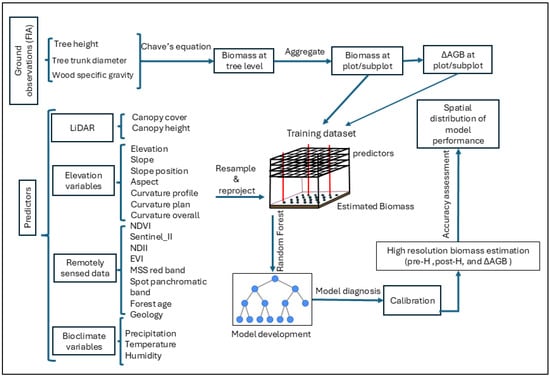
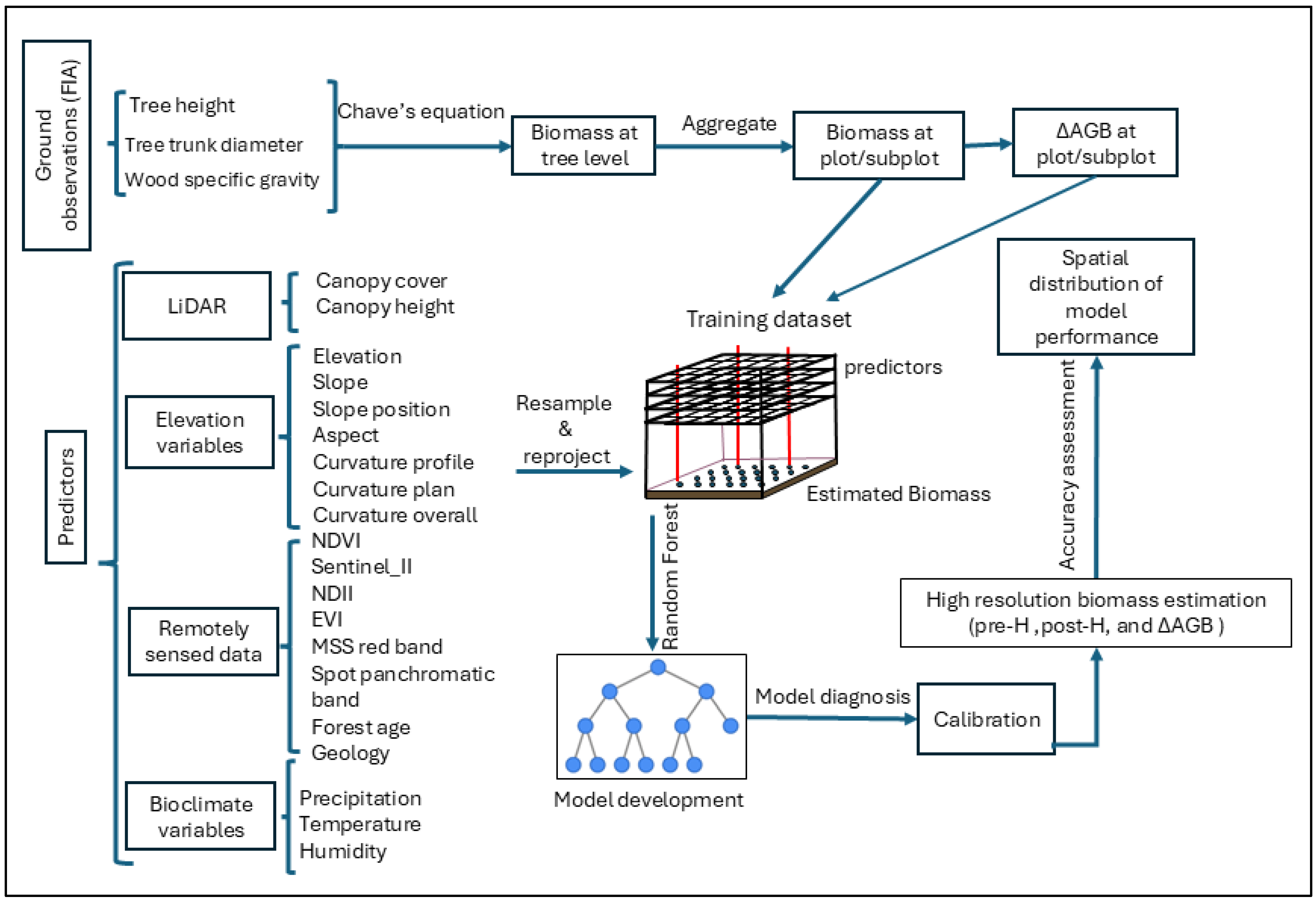
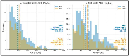
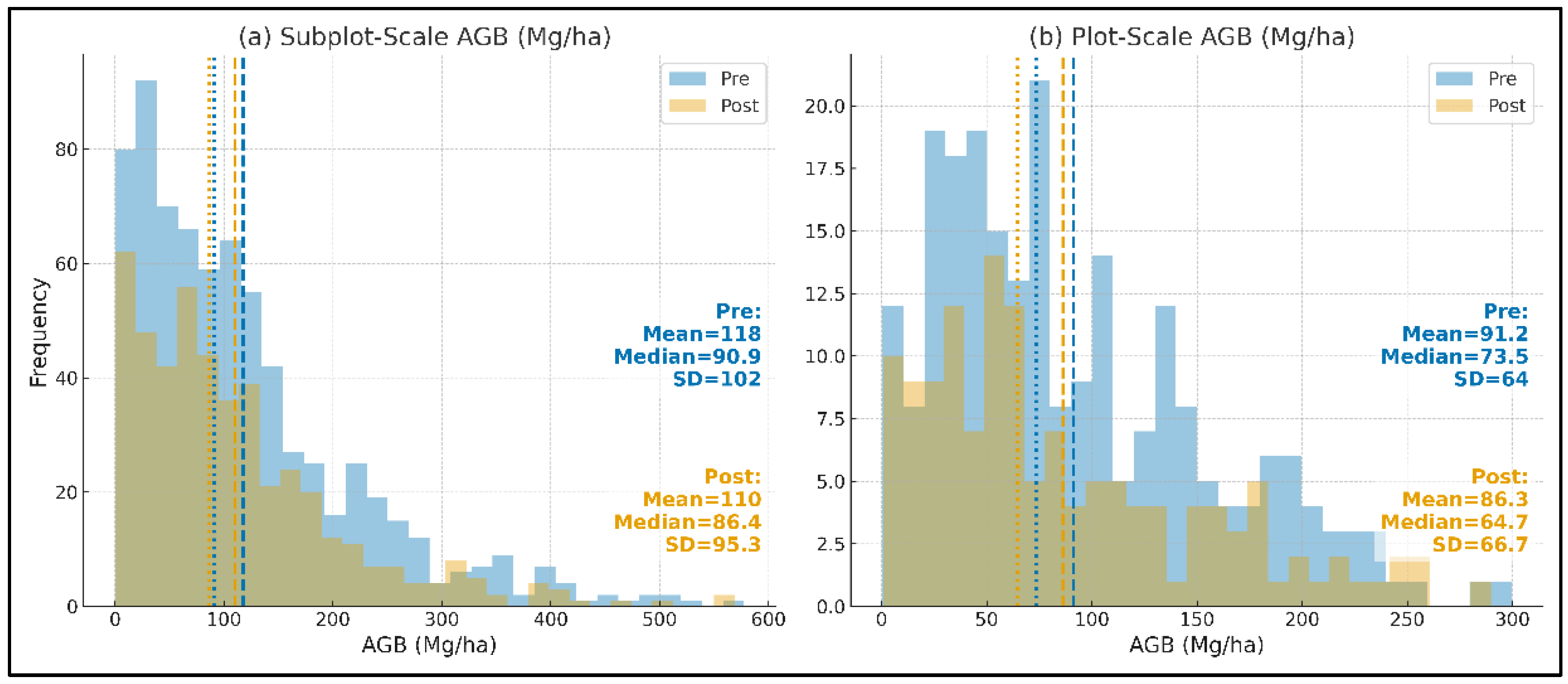
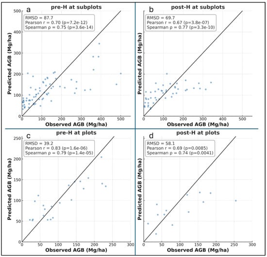
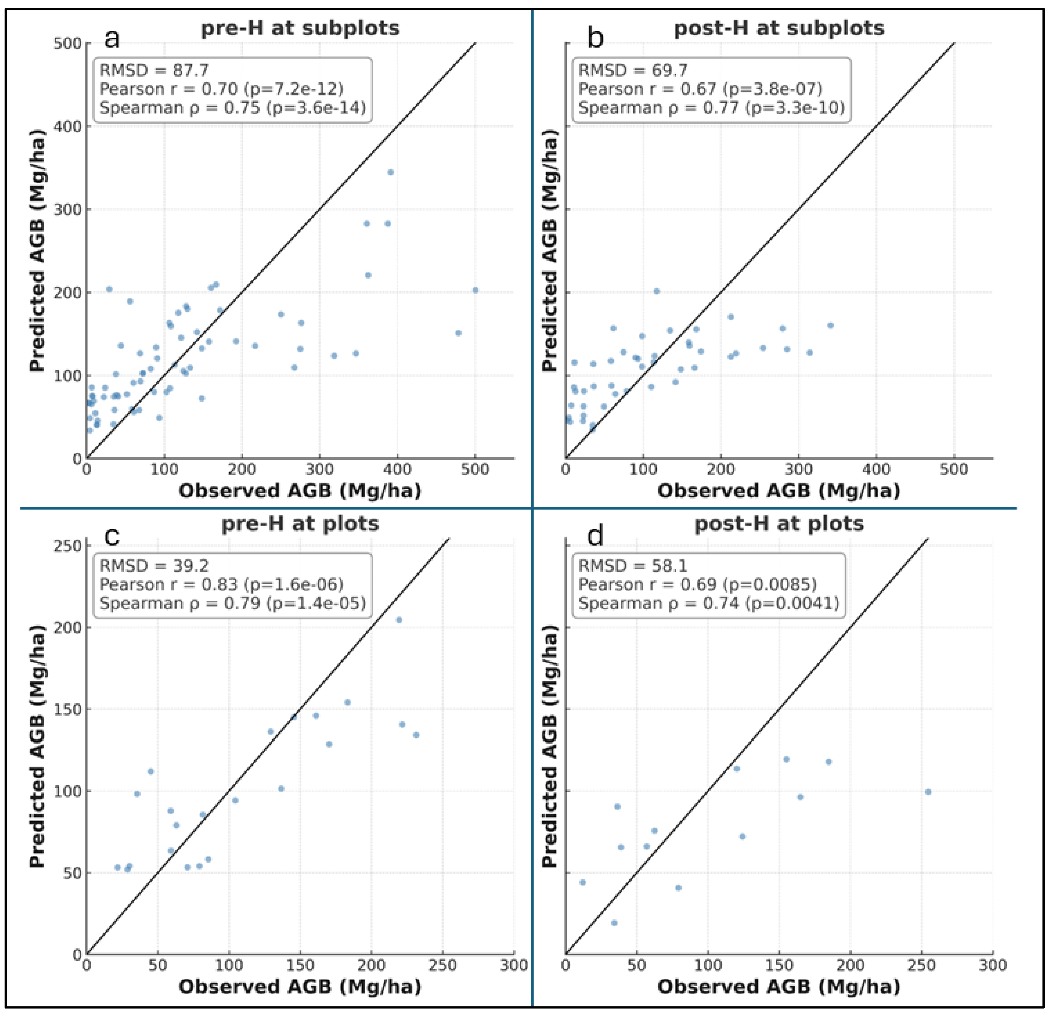
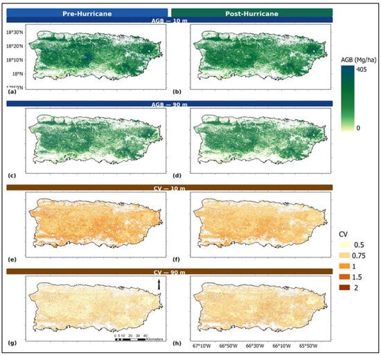
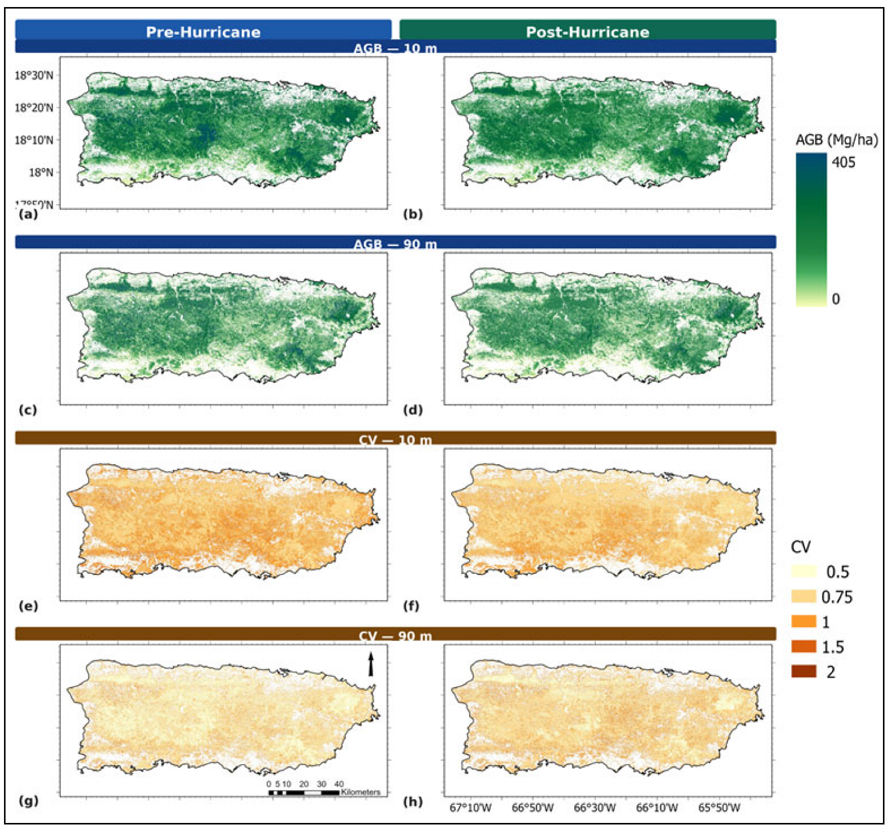
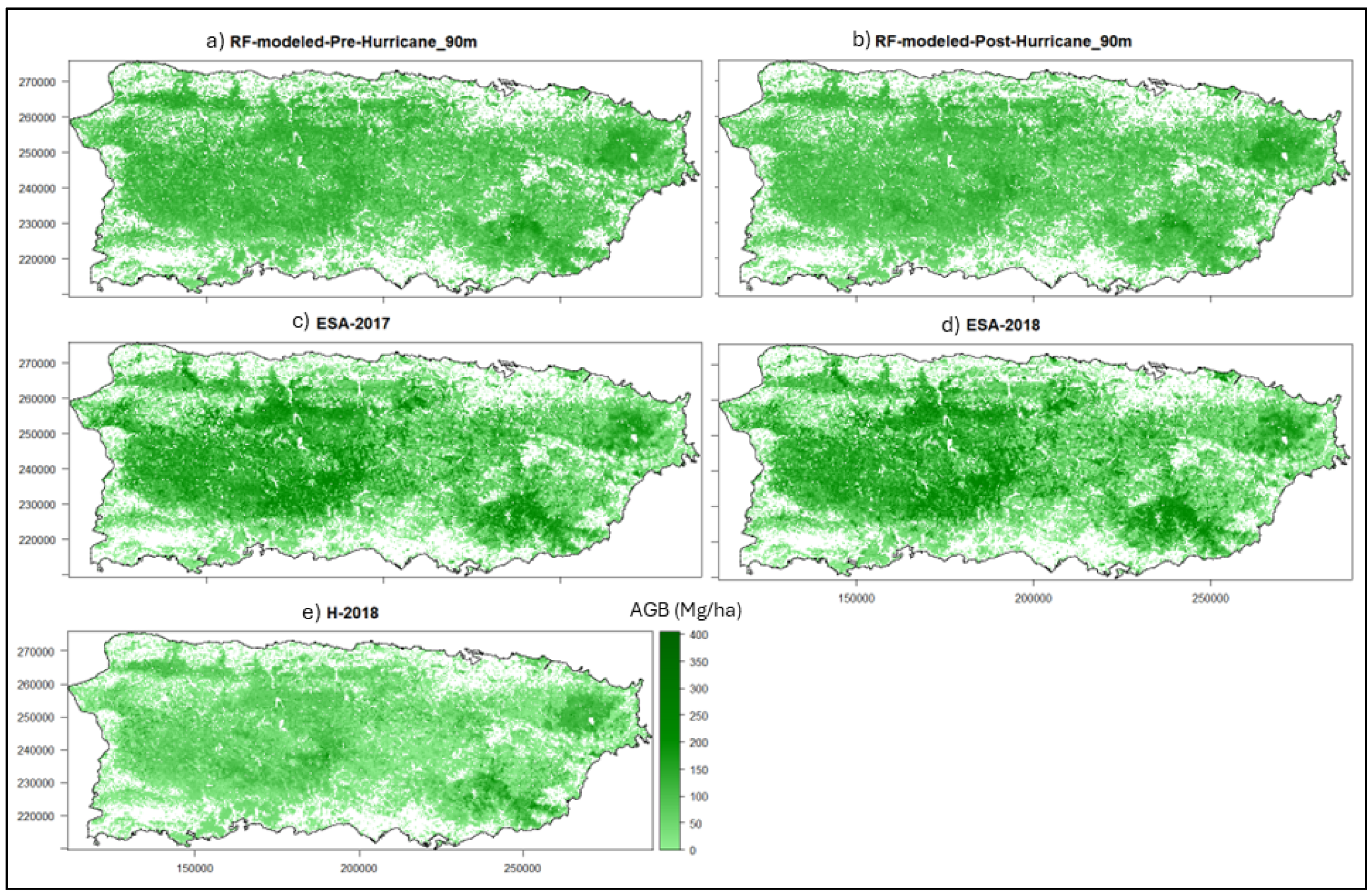
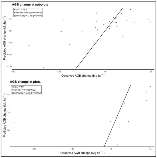
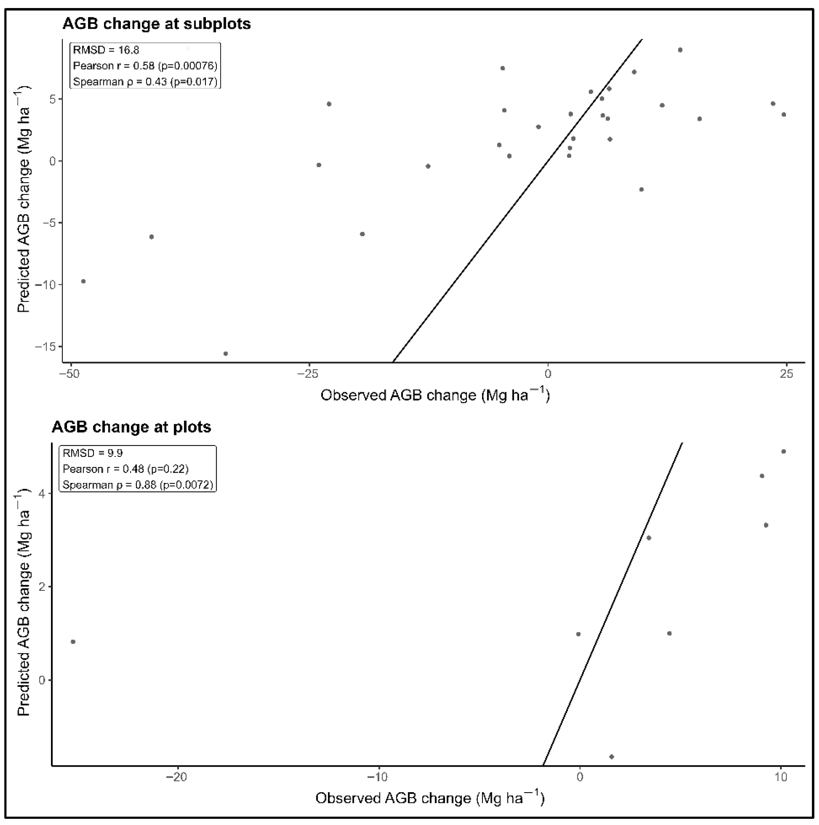
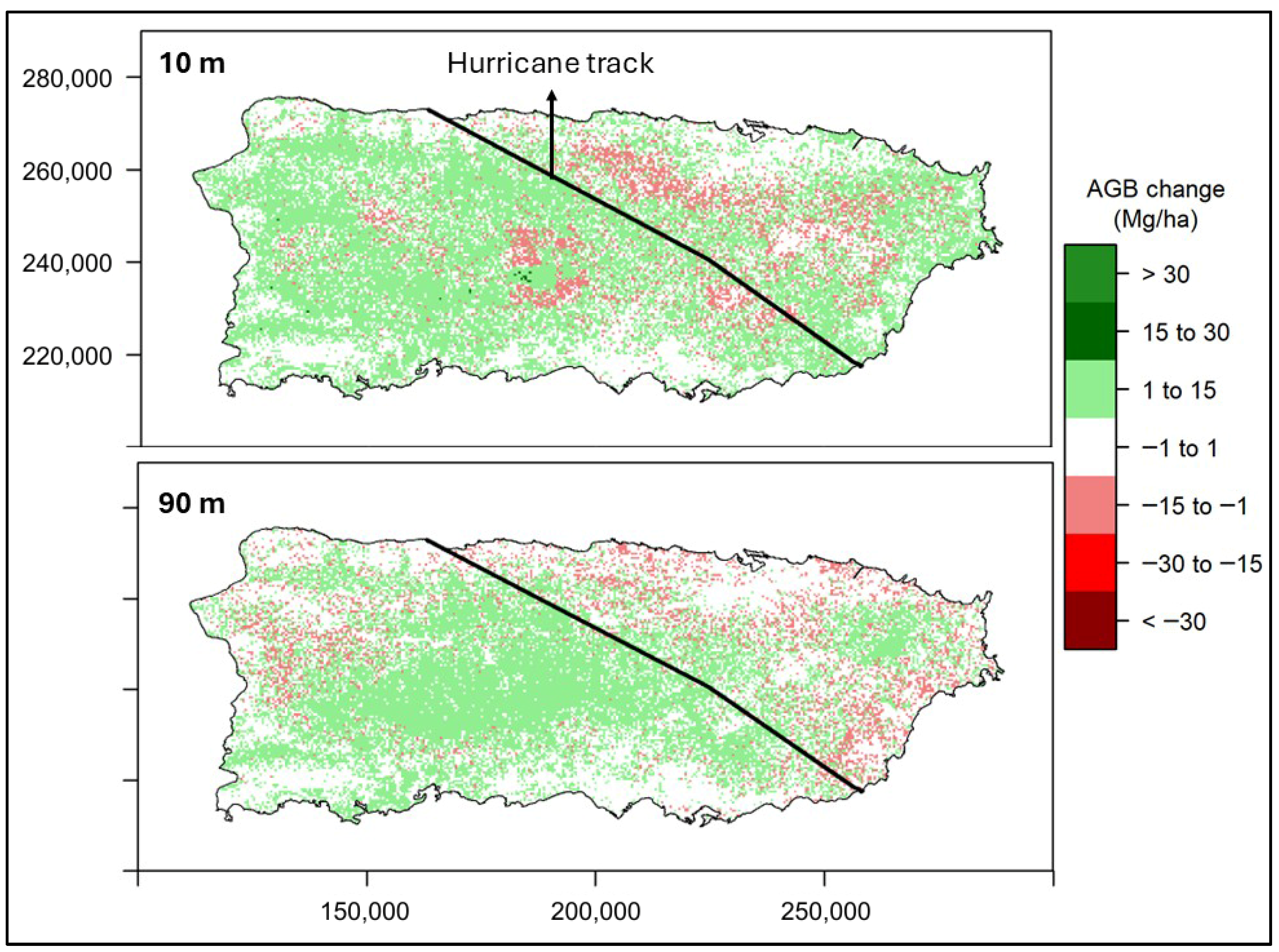

Disclaimer/Publisher’s Note: The statements, opinions and data contained in all publications are solely those of the individual author(s) and contributor(s) and not of MDPI and/or the editor(s). MDPI and/or the editor(s) disclaim responsibility for any injury to people or property resulting from any ideas, methods, instructions or products referred to in the content. |
© 2026 by the authors. Licensee MDPI, Basel, Switzerland. This article is an open access article distributed under the terms and conditions of the Creative Commons Attribution (CC BY) license.