


Highlights
What are the main findings?
- GMI 89 GHz single difference was characterized and filtered to provide a reference for TROPICS W-band cross-calibration.
- TROPICS–GMI double difference showed systematic dependencies on beam position, latitude, month, and measured brightness temperature.
What are the implications of the main findings?
- Residual double-difference dependencies are primarily associated with the TROPICS contribution, although measurement and modeling effects cannot yet be separated.
- The results demonstrate the utility of double difference cross-calibration for improving TROPICS W-band calibration and supporting calibration of future SmallSat radiometer constellations.
Abstract
The objective of this paper is to describe a robust technique to perform the inter-satellite radiometric calibration (XCAL) between two microwave radiometers of significantly different designs. Because this results in the relative calibration between the two, one is the reference and the other is the to-be-calibrated target. This technique makes no judgment as to which is the best absolute calibration; rather, it only considers the relative difference between the two. For our application, the Global Precipitation Measurement Microwave Imager (GMI) is the transfer standard for the inter-satellite radiometric calibration of a constellation of cooperative satellites’ microwave radiometers used to provide global precipitation measurements for an international community of scientific and operational users. This paper describes the on-orbit validation process for a future candidate GPM constellation member, namely, the 91.6-GHz TROPICS Pathfinder radiometer. A one-year TROPICS–GMI matchup dataset was developed using spatially and temporally collocated brightness temperature observations over clear-sky ocean scenes. Also, these brightness temperature data were combined with estimates of the associated environmental parameters, provided by a global numerical weather model product. The associated XCAL analysis procedures are described, and the radiometric bias results are presented.
1. Introduction
1.1. Satellite Microwave Radiometer Calibration
Satellite radiometry began in the mid-1960s, with NASA’s Nimbus program to develop remote sensing technology for scientific and weather applications, and microwave radiometers (MWRs) were among the early sensors developed. These early sensors were microwave imagers that relied upon relative radiance intensities (brightness temperatures Tb), and as a result, radiometer calibration was not an issue. However, in the late 1980s, the US Air Force weather satellite program, the Defense Meteorological Support Program (DMSP), launched the first operational microwave radiometer, namely, the Special Sensor—Microwave Imager (SSMI), and the availability of global, calibrated microwave radiances created the need for the development of inter-satellite radiometric calibration.
Today, there are numerous microwave radiometers operating on international weather and other remote sensing satellites. Most of these microwave radiometers (MWRs) are calibrated to provide absolute Tb measurements, so on-orbit radiometric calibration is a prime driver in MWR instrument design. A typical requirement is to measure the absolute radiance to within a few K, but the required measurement precision is usually <1 K.
Before launch, the MWRs are calibrated using precision blackbody sources applied at the receiver input under controlled isothermal environmental conditions. In most instances, the pre-launch calibration process does not involve the radiometer antenna; thus, the only end-to-end radiometer calibration occurs after deployment on-orbit. Furthermore, during the initial months of operation, the radiometer undergoes an aging process, whereby outgassing of water vapor and solvents occurs, causing subtle changes in the radiometer calibration. Also, the on-orbit thermal environment is cyclic with the orbit period and the one-year seasonal cycle. Because of this, at least a one-year period of on-orbit calibration/validation is an important requirement.
This paper describes a robust XCAL procedure, which is applied to a candidate MWR for inclusion in the Global Precipitation Program constellation of cooperative satellites. Before this candidate MWR is accepted into the GPM mission constellation, it must undergo rigorous radiometric scrutiny to assure that its Tb measurements are stable under the changing space environment. Moreover, the radiometric calibration is not absolute; rather, it is relative to the GPM Microwave Imager on the core observatory. However, because of significant differences in the constellation member MWR designs, a direct comparison of their Tb’s cannot provide the required radiometric bias necessary to include their Tb observations in the generation of satellite precipitation products.
This paper presents the details of the inter-satellite radiometric calibration of the TROPICS W-band MWR relative to the GMI 89 GHz channel. Because the antenna viewing geometries for these radiometers are considerably different (conical-scanning antenna for GMI and cross-track scanning through Nadir for Tropics), the radiometric intercomparison is not trivial. The technique employed is designed to account for known differences and to effectively normalize the brightness temperature observations (using a double difference technique) before inter-comparison. The principal objective of this paper is to describe the details of this XCAL evaluation, which can be universally used for other MWRs. The secondary objective is to present results for the XCAL radiometric biases of the TROPICS Pathfinder W-band channel.
1.2. GPM Mission
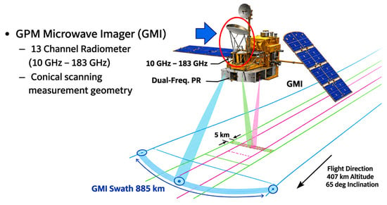
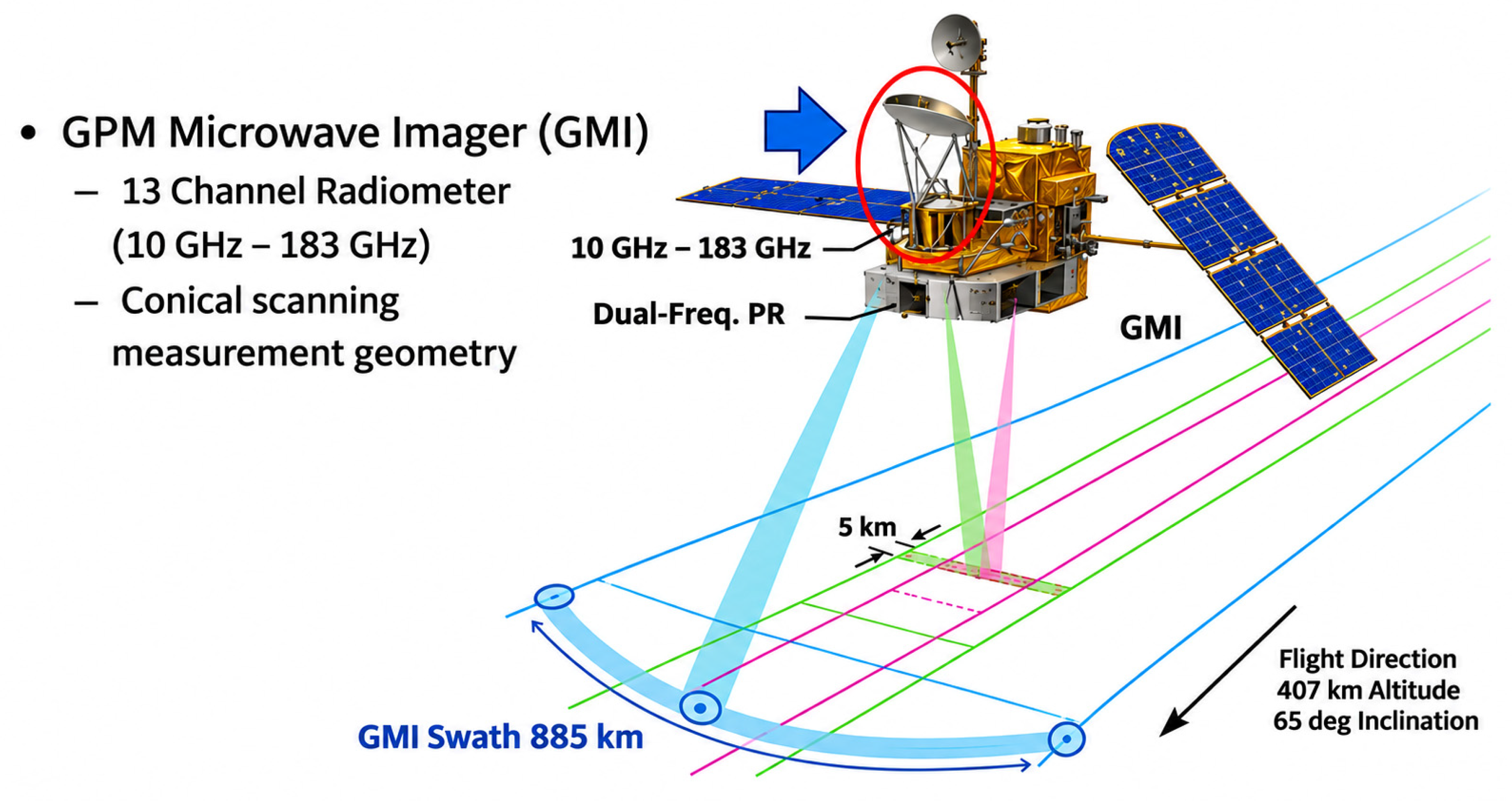
The Global Precipitation Measurement (GPM) observatory (Figure 1) is a joint NASA/JAXA remote sensing satellite that has two prime sensors, namely the JAXA Dual-frequency Precipitation Radar (DPR) and the NASA GPM Microwave Imager (GMI), and this paper concerns only the latter. This dedicated satellite precipitation measurements program began with the launch of the Tropical Rainfall Measurement Mission (TRMM) in 1997, and it was extended by the follow-on GPM Mission in 2014. Thus, this program has provided more than three decades of global precipitation measurements to an international community of scientific and operational users. The GPM core observatory operates in a low-Earth orbit, which is augmented by a constellation of existing international satellites carrying MWRs.
Figure 1.
GPM Core Observatory showing the Dual-frequency Precipitation Radar (DPR) and GPM Microwave Imager (GMI) measurement swaths. Image credit: NASA and adapted for clarity.
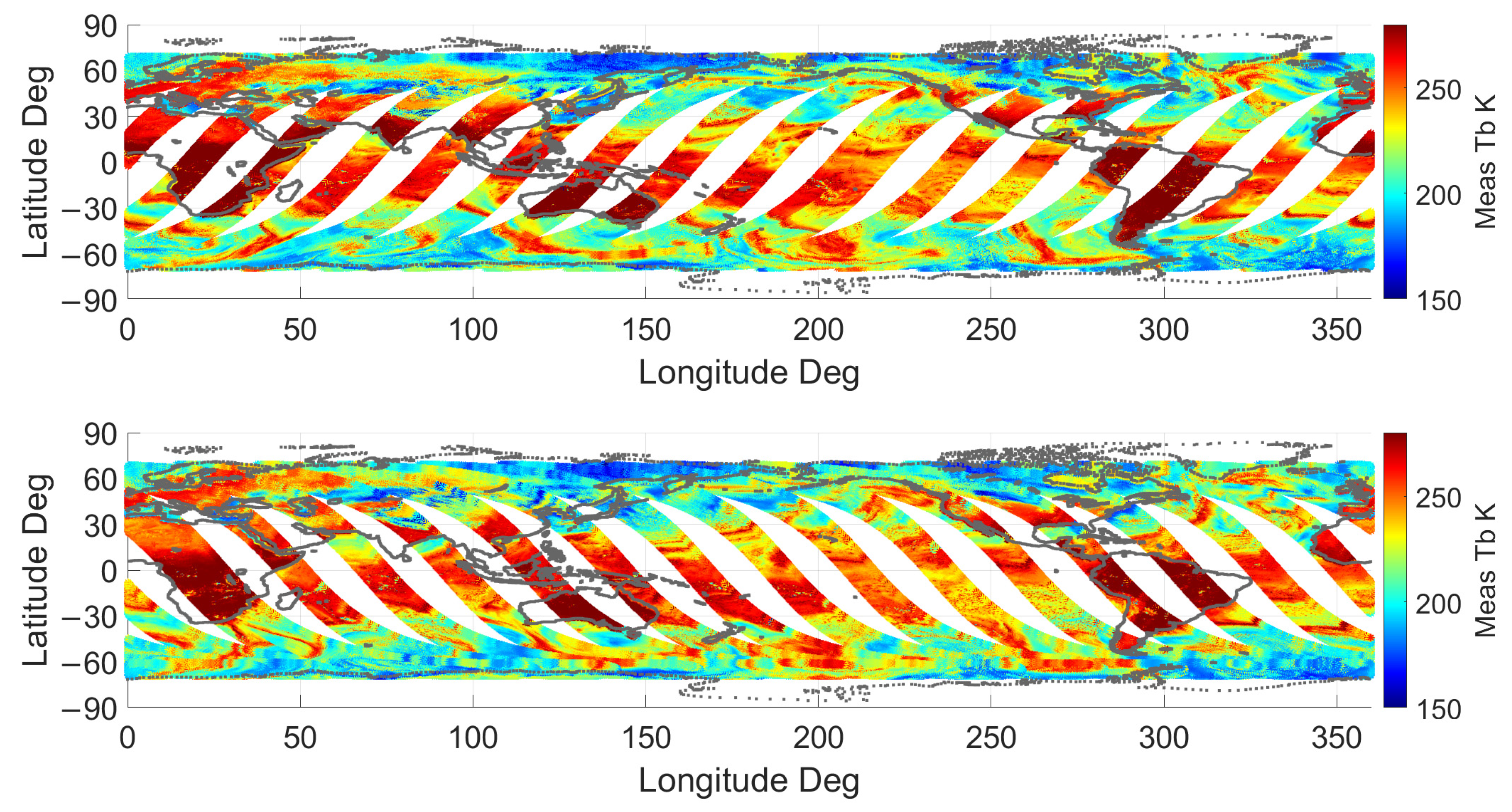
GMI is a microwave radiometer imager with 13 channels ranging from 10 to 183 GHz, but for this paper, only the 89 GHz dual linearly polarized vertical (V-) and horizontal (H-) channels are used. The GMI offset-fed reflector antenna produces separate antenna beams by channel, which are mechanically rotated using a conical scanning geometry with an Earth incidence angle of 53°, which results in a measurement swath width of about 900 km. The 89 GHz antenna instantaneous field of view (IFOV) on the surface is approximately 4 × 7 km, and an image of H-pol brightness temperature for one day is shown in Figure 2, with descending and ascending passes separated.
Figure 2.
GMI 89 GHz H-pol Tb observations for 19 January 2022, where the upper panel shows the ascending orbital passes and the lower panel shows the corresponding descending passes. The color bar is measured Tb in Kelvin.
The GPM core observatory operates in a low-Earth altitude (407 km) orbit with an inclination of 65°, and the individual swaths have observation gaps between orbits. The GMI samples about 80% of oceans at least once per day (between ± 65° latitude), and many of these points at latitudes > 30° are sampled twice (~12 h apart). Moreover, during the next day, the orbit precession causes the measurement swath to cover the previous missing observations. Thus, after 2 days, there is almost total ocean coverage between ± 65° latitude, with most locations having 2 or more revisits.
Because the absolute radiometric calibration of GMI is superior [1], it serves as the precipitation measurement standard for the other GPM constellation satellites. Since most of the constellation satellites are in sun-synchronous (sun-syn) orbits, their local observation times are the same each day. Since the GPM core observatory operates in a non-sun-synchronous orbit, the GMI measurement swath crosses the constellation member swaths twice daily at their local times (day and night). However, the corresponding GMI times are not coincident, and this differential observation time varies progressively each day as a result of differences in the orbit periods. Nevertheless, every constellation satellite has multiple (~30) crossings daily within a differential time of ±1 GPM orbit (~93 min). Furthermore, only the GMI intersects the measurement swaths of all the constellation members; therefore, it serves as the radiometric calibration transfer standard. It is important to note that constellation satellites collaborate by providing their microwave Tb observations (not precipitation measurements), and the XCAL of the constellation MWRs and the production of the GPM precipitation products is solely the responsibility of the GPM project at the NASA Goddard Space Flight Center in Greenbelt, MD.
Concerning global precipitation products, there are many operational users (e.g., international weather services), who require near real-time precipitation observations to issue their forecasts of severe precipitation events. Over land, there are numerous land-based meteorological radar networks that provide these data, but over oceans, no such global-wide network exists. Thus, the international operational weather community relies heavily on remote sensing satellites to provide these near real-time precipitation observations.
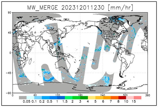
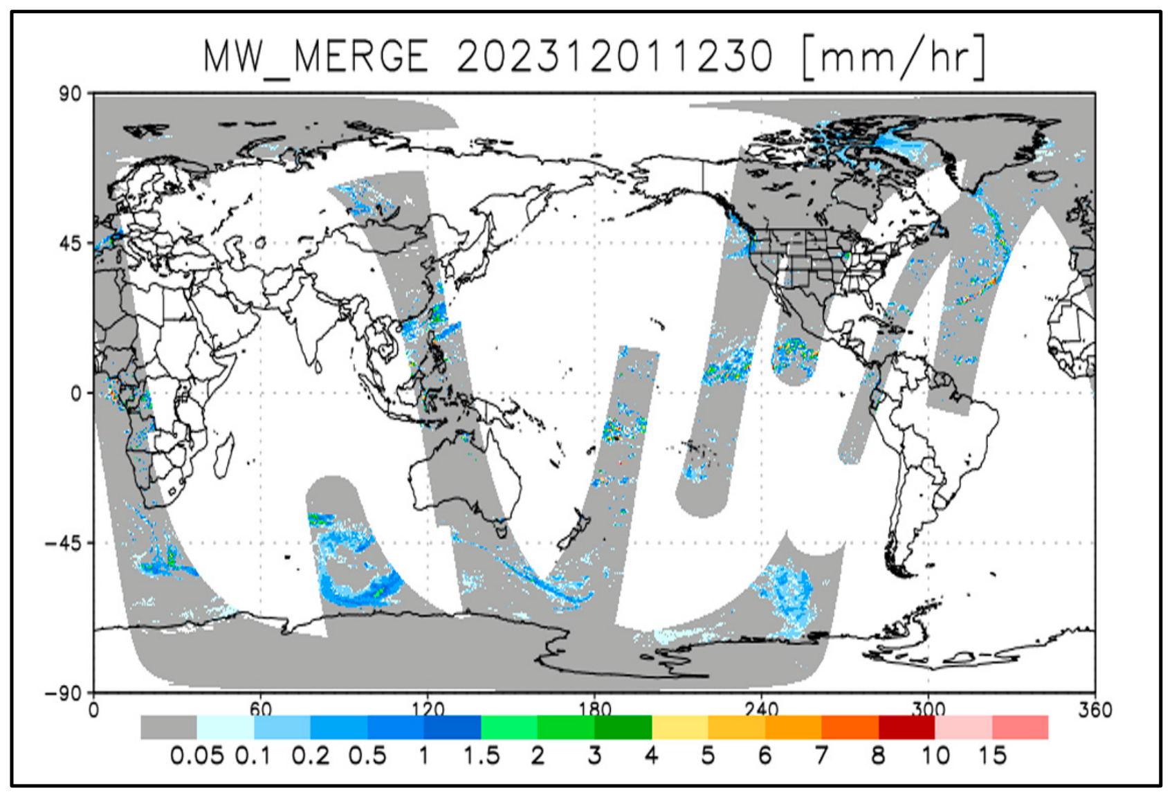
Thus, the GPM program provides diverse precipitation products and among these is the Integrated Multi-satellite Retrievals (IMERG) [2,3], which provides global rainfall measurements in 30 min intervals. Unfortunately, within this 30 min interval, the GMI can provide only about 5% of the required global coverage; therefore, the GPM program has adopted a constellation of cooperative satellites using MWRs and visible/infrared (VIR) imaging sensors that provide the desired global precipitation measurements. A typical example of the spatial coverage provided by the GPM constellation within a 30 min interval is shown in Figure 3. The gray shaded area (~ 40%) represents the precipitation estimates provided by nine MWR constellation satellites, and the white area (~ 60%) is the remaining coverage of only GOES VIR images. Note that the TROPICS satellite is not part of the existing GPM constellation; however, because of its wide swath, it has the potential to significantly improve the MWR coverage.
Figure 3.
Example of typical oceanic coverage (~40%) provided by GPM constellation MWR observations for the IMERG 30 min interval product. Figure courtesy of NASA.
This is advantageous because the VIR sensors cannot penetrate rain clouds, and therefore, the precipitation estimates are indirect, based upon statistical correlations between visible cloud-top brightness and infrared temperature. On the other hand, MWR precipitation retrievals are superior because they are based upon the integral of rainfall blackbody emissions, from which an average rain rate measurement is retrieved.
However, since the GPM constellation includes MWRs with varying frequencies and observation geometries, it is necessary that their relative radiometric calibration (with respect to GMI) be determined. Approximately half of these comparisons involve the XCAL between similar conical scanning MWRs, and the remaining involve XCAL with cross-track scanning MWRs.
This paper focuses on the latter, which are more challenging because of the vastly different Tb observation geometry. The associated XCAL procedure is described, and results from the on-orbit XCAL radiometric calibration bias between the TROPICS 91.6 GHz channel and the GMI 89 GHz channel are given.
1.3. TROPICS Mission
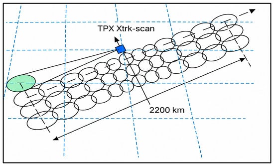
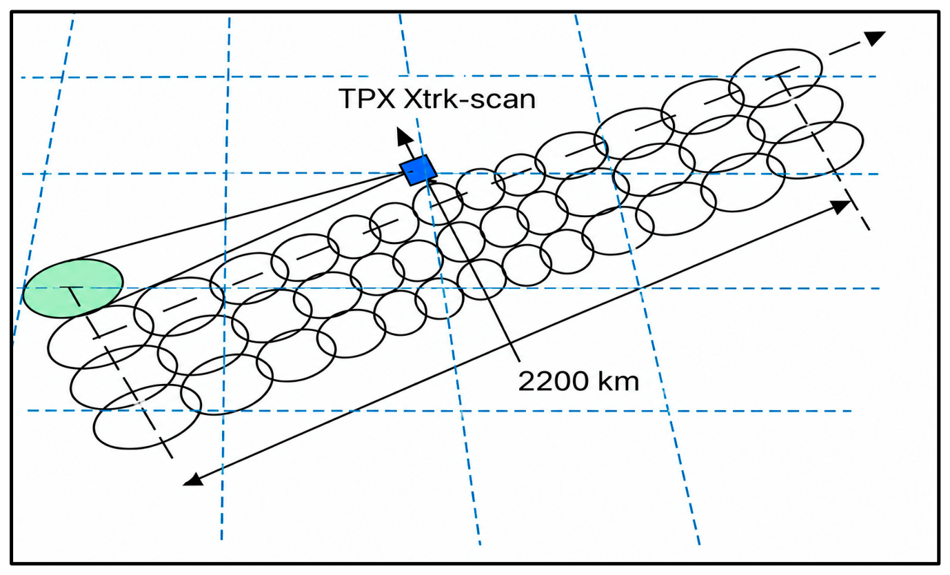
This paper focuses on the TROPICS Pathfinder satellite, which operates in a sun-synchronous low-Earth orbit. The Time-Resolved Observations of Precipitation structure and storm Intensity with a Constellation of Smallsats (TROPICS, hereafter TPX) is a NASA satellite mission designed to provide frequent observations of tropical cyclones. TPX is a constellation of 4 small satellites equipped with two cross-track scanning MWRs, each with 81 cross-track pixels for a swath width of 2200 km. The cross-track geometry produces a variable Earth incidence angle (EIA) and IFOV across the sensor swath, as shown in Figure 4. Along the satellite nadir track (beam position 41), the 91.6 GHz antenna IFOV is ~29.6 km, and this monotonically increases to 75 km across track by 45 km along track at beam positions 9 and 72, which match GMI EIA (see Table 1 for IFOV at different EIA). The advantage of TROPICS’ wide swath is that it provides almost contiguous sampling of precipitation, and the use of 4 satellites, 3 of which operate in low-Earth non-sun synchronous orbits, improves global temporal sampling, which could significantly benefit the GPM IMERG precipitation product. Each day, the TPX imager provides near-full global coverage during both the ascending and descending portions of its orbit, as shown below in Figure 5.
Figure 4.
TROPICS cross-track scanning geometry with 81 cross-track Tb observations (beam positions).
Table 1.
Estimated TPX footprint variation with incidence angle.
Figure 5.
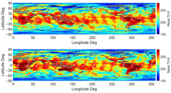
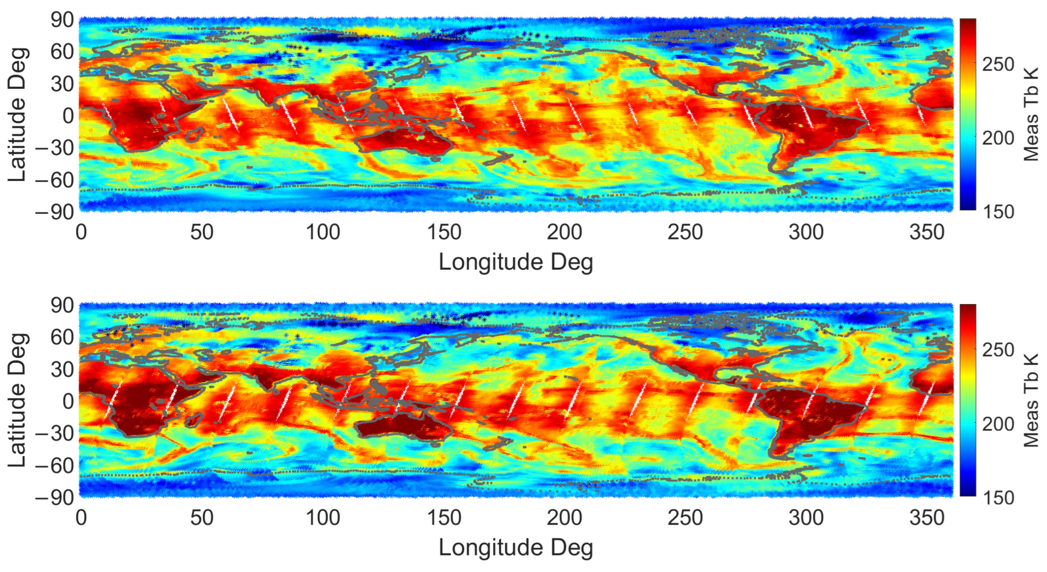
TPX 91.6-GHz measurement swaths for ascending and descending passes on 19 January 2022. The color bar is Tb in Kelvin.
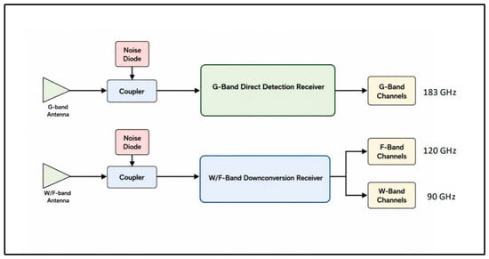
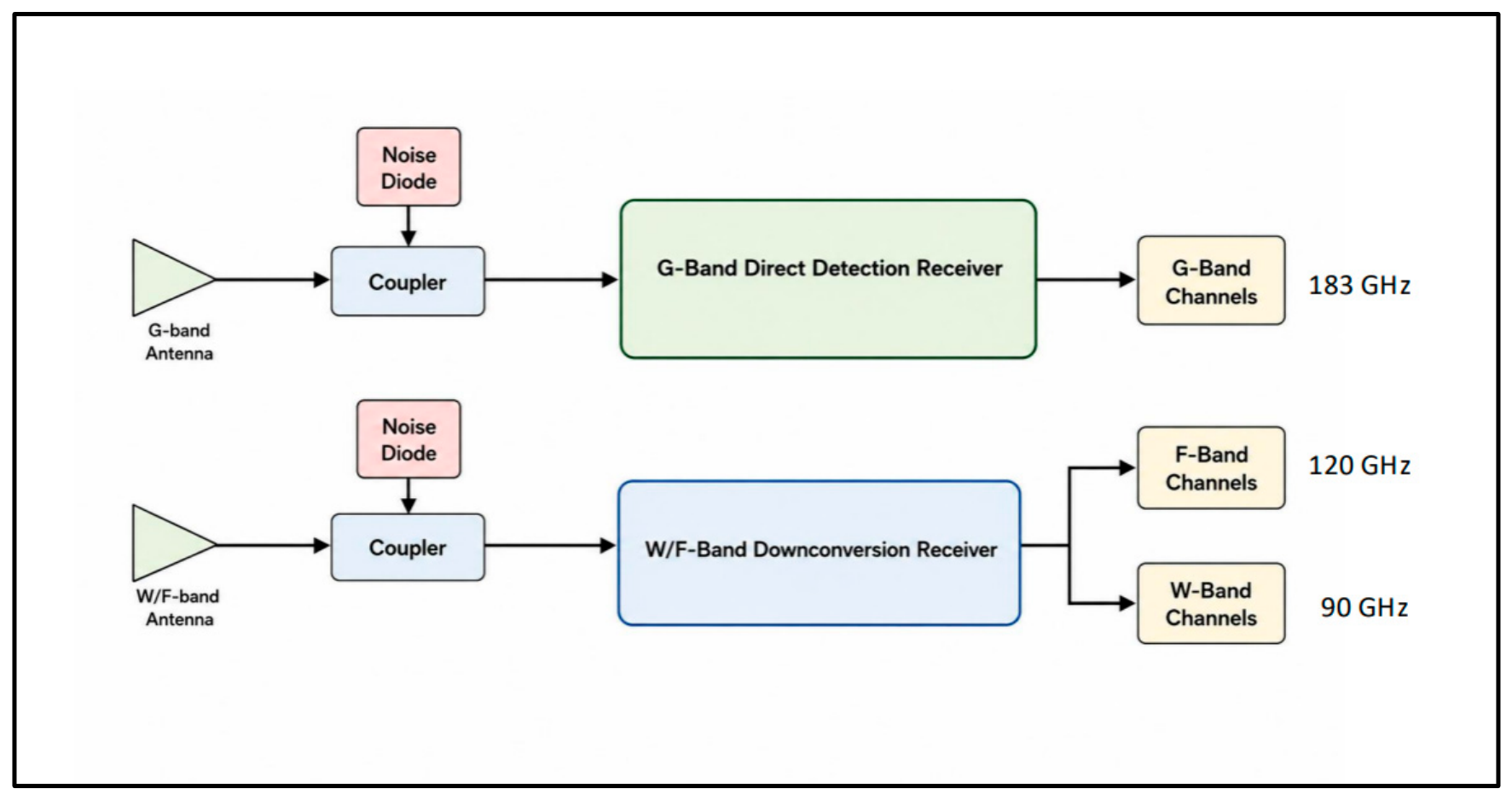
The TPX sensor package, depicted in Figure 6, comprises two total power radiometers (W/F-band and G-band) with noise diode injection calibration, but for this paper, only observations from the W-band channel are used. The W/F-band radiometer uses a heterodyne down-conversion receiver, with the W-band operating in double-sideband mode and the F-band operating in single-sideband mode.
Figure 6.
TPX sensor block diagram for W/F-band and G-band total power radiometers.
These radiometers share a common offset reflector with separate orthogonally polarized feeds, which results in two high beam efficiency antenna patterns. However, because of a small misalignment with respect to the normal to the surface, this results in a cross-pol mixing ratio of 94.6% horizontal and 5.4% vertical for the W/F-band. Unlike most cross-track sounders, for which the polarization orientation rotates with scan angle, the polarization of the TPX channels remains constant across all viewing angles.
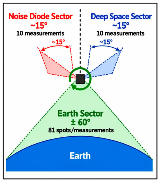
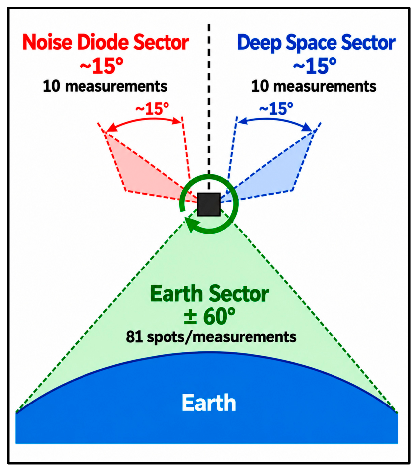
An important radiometric calibration advantage is that the entire TPX radiometer assembly (antenna and receiver) is mechanically rotated to make radiance measurements of space and Earth. During each scan (2 s), the instrument collects 10 noise-diode, 10 space, and 81 cross-track Earth-scene measurements (Figure 7).
Figure 7.
TPX Tb measurement sequence during a single antenna scan. The first sector views space with the noise diode on, the second sector views space with the noise diode off, and the last sector views the Earth scene in 81 beam positions.
2. Materials and Methods
This section describes the development of the GMI–TPX match-up dataset and the XCAL processing used to evaluate the TPX XCAL radiometric bias (Inter-satellite Radiometric Calibration).
2.1. Match-Up Dataset for TPX-GMI
As discussed in Section 1.2, the GPM XCAL procedure is used to provide inter-satellite radiometric calibration of the GPM constellation microwave radiometers. This is necessary to ensure the uniformity of the constellation brightness temperatures (Tb’s) used in the IMERG precipitation retrievals. In this section, the generic XCAL procedure is described, and details are given about the production of the GMI/Target radiometer match-up dataset that is used to estimate the radiometric bias of a target radiometer channel relative to the corresponding GMI channel.
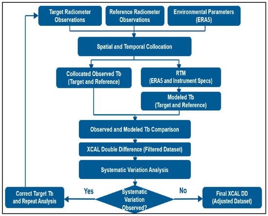
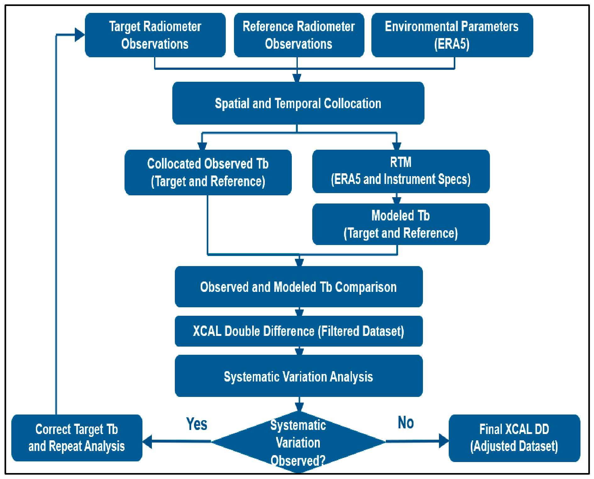
A block diagram of the XCAL processing procedure is shown in Figure 8, where the GMI is the reference instrument and the constellation MWR is designated as the target.
Figure 8.
Inter-satellite Radiometric Calibration (XCAL) procedure.
First, reference and target MWR Tb’s are spatially and temporally collocated on a 0.5° latitude/longitude grid (boxes) over oceans. This spatial collocation involves GMI and TPX Tbs whose IFOV centers fall within the grid box. Typically, the GMI IFOVs are uniformly distributed across the box, but as noted above (see Table 1), most TPX IFOVs extend outside the area of the box. However, the rationale for selecting a 0.5° box is to limit the number of TPX beam positions within each box to only 5, which restricts the EIA to the mean ± 3°. The temporal window for GMI/TPX match-ups is within 120 min of the GMI observations, and the corresponding environmental parameters, from the European Centre for Medium-Range Weather Forecasts fifth-generation reanalysis (ERA5) global numerical weather product, are added. For each box, ERA5 data are spatially interpolated to the box center.
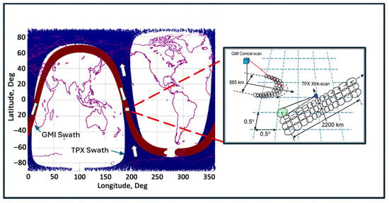
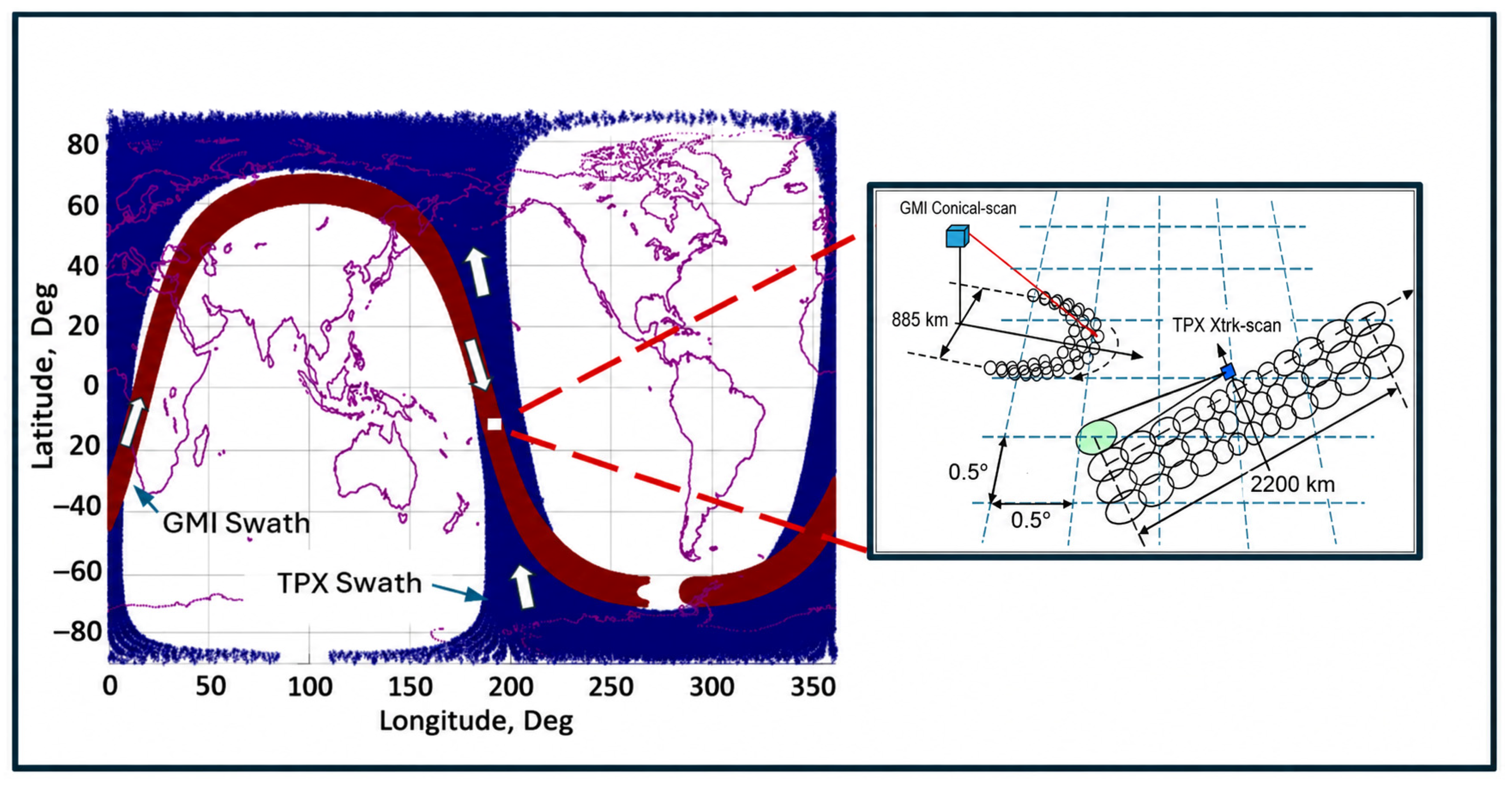
At this point, we switch from the generic comparison to using the TPX W-band 91.6 GHz channel as the target and the GMI 89 GHz V- and H-pol channels as the reference. An example of the GMI/TPX collocations for one GMI orbit (red swath) is shown in Figure 9. Also shown, as an insert (right-hand panel), is an illustration of the spatial match-up of GMI and TPX Tb pixels. Within these 0.5° boxes, the typical number of Tb measurements is 6 for TPX and 40 for GMI, and these Tb measurements are averaged to produce box average values. Tb averaging is desired to reduce the random single measurement noise equivalent delta-T (NEDT), thereby providing an improved estimate of the collocated Tb. Also, note that these matchups typically occur for only about one-quarter of a single GMI orbital pass between ± 65° latitude, and specifically, for this case, the descending GMI orbit segment is collocated with the TPX ascending orbit segment. Furthermore, over the period of one month, all combinations of GMI and TPX ascending and descending orbit segments do occur. Also, since TPX Pathfinder operates in a sun-synchronous orbit, these collocations are separable into day/night passes.
Figure 9.
Typical spatial collocation for GMI (red) and TPX (blue) observations for a single TPX ascending and GMI descending orbit segment. The figure insert (right panel) illustrates the geometric relationship between the observed Tbs for GMI (conical scan) and TPX (cross-track scan).
2.2. Double Differences XCAL Methodology
The Central Florida Remote Sensing Laboratory has developed the double difference (DD) technique [4,5,6,7,8] to perform inter-satellite radiometric calibration for the TRMM/GPM program. Based on two decades of comparisons between conical scanning MWRs, the precision of the estimate of the XCAL bias is typically a few tenths of a Kelvin. However, based on similar XCAL DD comparisons between conical scanning and cross-track scanning MWRs [9,10,11], the uncertainty of the XCAL biases is typically greater than ±1 Kelvin. We interpret these results to mean that the XCAL radiative transfer model (RTM) accurately predicts the measured Tbs over a wide range of environmental conditions, provided that the MWR Tb measurement geometries are similar. In the cross-track scanning cases, where the MWR EIAs are significantly different, we conclude that the precision of the XCAL bias estimates is degraded because of RTM modeling of the rough surface ocean emissivity over EIA.
Moreover, in both cases, on infrequent occasions, the DD values significantly change, and these are hypothesized to be associated with either random measurement errors or bad environmental parameters from the numerical weather model. Regardless of the cause, these Tb observations are anomalous and are rejected from the XCAL process. So, the removal of these anomalous data is described in Section 2.4. By using thousands of independent match-ups, the Central Limit Theorem applies, and our hypothesis is that the target MWR XCAL bias is a Gaussian probability distribution about the “true” Tb DD bias.
So, using a preliminary match-up dataset of 3 months, a systematic analysis is performed to validate this assumption. To perform this statistical test, the XCAL DD is averaged by latitude, by month and by measured Tb. If the DD average value is generally constant, regardless of how the data are sorted and averaged, then the hypothesis is confirmed. Afterwards, the XCAL process continues for the one-year match-up dataset, and the resulting average DD and its associated uncertainty is the XCAL bias.
On the other hand, if this hypothesis testing fails (i.e., the XCAL DD is not constant), then the XCAL process cannot continue until the root cause of this variability is determined and corrected. Often, this systematic bias variability can be corrected on an ad hoc basis with some other instrument parameters (e.g., the MWR physical temperature). After this, the hypothesis testing is reevaluated with the one-year modified dataset, which covers the full seasonal cycle of environmental parameters.
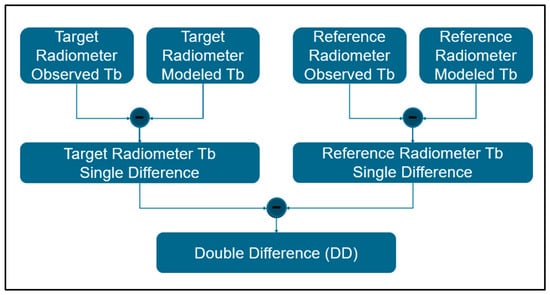
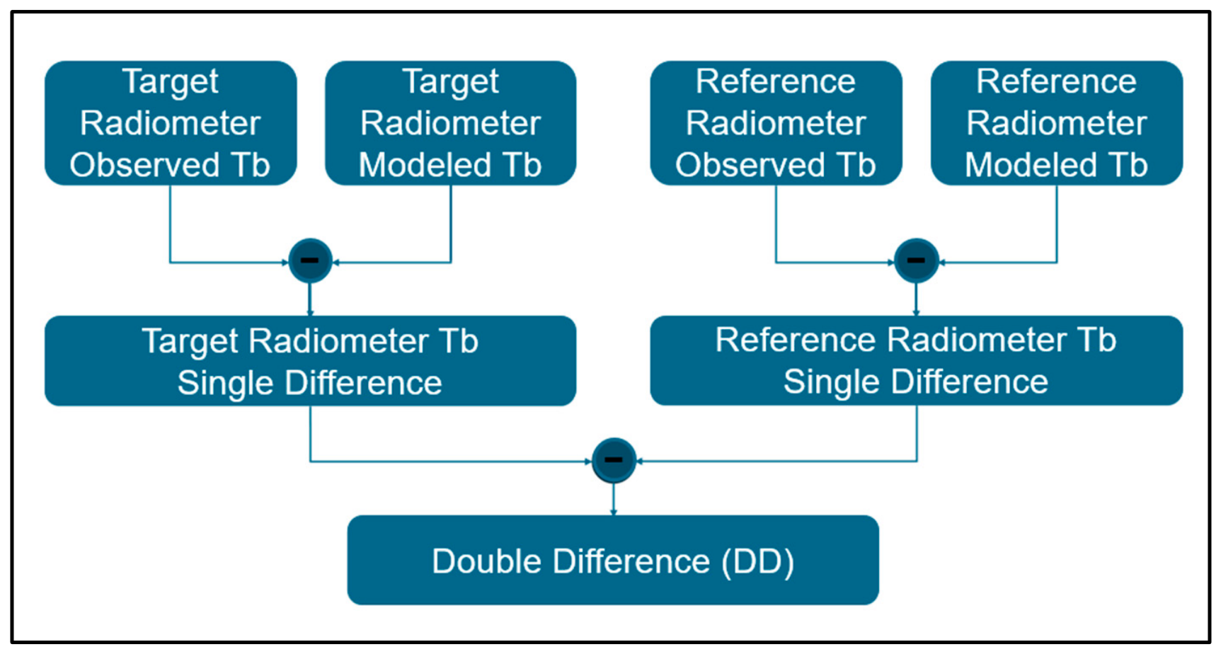
The double difference procedure (illustrated in Figure 10) uses single differences (SD) between the observed Tb and the modeled Tb that are calculated for both target (TPX) and reference (GMI) MWRs. The XCAL bias is the double difference between the Target SD and the Reference SD. Alternatively, the DD can also be calculated using the differences of the observed Tbs (OSD) and modeled Tbs (MSD).
Figure 10.
The XCAL double difference calculated using the single differences between the target and reference radiometers.
Usually, the brightness temperatures measured by two satellite instruments within the same collocated box cannot be directly compared because of differences in geometry and radiometric parameters, which produce differences in the measured brightness temperatures even in the absence of calibration errors. To account for these differences, the RTM is used to model the expected brightness temperature for each instrument based on its observation geometry, frequency, polarization and the corresponding atmospheric and oceanic environmental conditions. The single difference between the two modeled brightness temperatures (MSD) represents the expected difference between the measurements. Thus, the double difference, between the observed brightness temperature single difference and the modeled brightness temperature single difference, is the XCAL radiometric bias between the two instruments. Thus, using this double-differencing approach, the expected differences, between the observations and other common-mode errors, should cancel and thereby yield the desired estimate of the radiometric bias. On the other hand, given previous experience with cross-track sounder XCAL [9,10,11], it is reasonable to expect some small residual uncertainty in the DD may exist, which is associated with common-mode sources that do not fully cancel.
2.3. Radiative Transfer Model
As described above, a one-year match-up dataset of GMI and TPX Tb observations and associated ERA5 environmental data is developed. For every box, the XCAL consensus radiative transfer model (MonoRTM), described by Biswas et al. [4] and De La Llana et al. [11], is used to model the theoretical Tb for both GMI and TPX. This RTM uses 100 equal layers from the surface to 20 km altitude to calculate the top of the atmosphere, linearly polarized microwave Tb for a clear-sky ocean scene as a function of the EIA between nadir and 65°, which is applicable for TPX beam positions between 4 and 77. Over this range of EIA, the smooth ocean surface reflection coefficient follows Fresnel theory, and the surface emissivity model [12] includes an ocean complex dielectric constant model that is a function of microwave frequency, sea surface temperature and salinity. Also, the model includes an empirical rough-surface diffuse scattering model associated with small-scale ocean waves (surface wind speed).
For the atmosphere, refraction effects are negligible and path length within the troposphere is calculated using spherical Earth geometry. The RTM uses atmospheric absorption coefficients that are a function of microwave frequency and environmental parameters, namely thermodynamic temperature, molecular densities of water vapor (WV), oxygen, nitrogen and cloud liquid water (CLW) as a function of altitude. However, the RTM does not include scattering by cloud ice or rain. Therefore, these effects are not captured in the modeled brightness temperatures. Thus, their influence is limited through the additional environmental screening and filtering procedures described in Section 2.4.
The GMI channel has a bandwidth of 6 GHz centered at 89.0 GHz, and the TPX W-band channel has a bandwidth of 1 GHz that is centered at 91.7 GHz. MonoRTM simulations were performed across the respective channel bandwidths, with the simulated brightness temperatures weighted according to each instrument’s Spectral Response Function (SRF). The simulations used nominal center frequencies of 89.0 GHz for GMI and 91.7 GHz for TPX W-band. Because the atmospheric absorption spectrum in this frequency region is relatively smooth without molecular resonance features, there are negligible differences in the Tb over the passbands for the same atmospheric path. On the other hand, when considering the atmospheric absorption/emission change between nadir and the GMI 52.8°, the effects are large but highly predictable, given near-homogeneous atmospheric conditions within the 0.5° box.
Before calculating the single difference and double difference, the GMI H- and V-polarization brightness temperatures are combined using the TPX W-band polarization mixing ratio of 94.6% H-pol and 5.4% V-pol. This accounts for the different polarization responses of the instruments, while their respective viewing geometries and center frequencies are represented in the RTM simulations. The resulting channel-specific modeled Tb values are then paired with the corresponding observed Tb values for the XCAL DD analysis.
2.4. Data Screening and Quality Control (QC) Filters
2.4.1. Nominal XCAL Data Screening Criteria
For any GPM constellation MWR, the XCAL DD bias can be any value; however, the uncertainty of this bias value must be known. The reason for this is that the precipitation retrieval using constellation MWR observations requires both the mean and the error (standard deviation) of the MWR Tb bias relative to the associated GMI channel. The XCAL goal for the knowledge of the bias uncertainty (i.e., the precision of the estimated DD value) is <0.1 K [10]. However, in practice, the typical XCAL DD bias uncertainty estimate exceeds several tenths of a Kelvin, but the upper limit of XCAL bias uncertainty cannot exceed 1 K. Therefore, to reduce this uncertainty, the XCAL evaluation dataset is restricted to only the highest quality match-up observations available. Specifically, land and ice scenes are removed because of their large uncertainties in surface emissivity and physical temperature. Moreover, for oceans, only spatially homogeneous, clear-sky scenes are used for XCAL purposes. These conditions are achieved by using a series of data QC filters described below.
The first QC filter, designed to assure spatial homogeneity of environmental parameters within the 0.5° match-up box, uses only GMI Tb observations. Because of the reduced IFOV size and the uniform spatial distribution of observations within the box, it is possible to estimate spatial gradients of environmental parameters from the standard deviation of the box average Tb measurement. This filter removes boxes, where the GMI Tb standard deviations are >2 K for V-pol and/or >3 K for H-pol.
Next, because clouds are spatially heterogeneous and temporally variable on time scales of an hour, it is highly desirable to remove cloud-covered oceanic scenes. For this purpose, the ERA-5 value of cloud liquid water is used to remove boxes for CLW > 0.1 mm. Also, because of imperfect cloud detection from ERA5, using these filters may result in some cloud-contaminated scenes remaining in the dataset, and this possibility is addressed in Section 2.4.2.
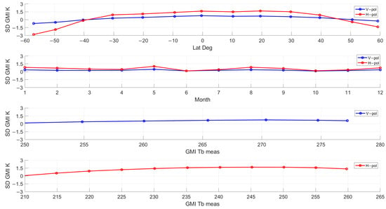
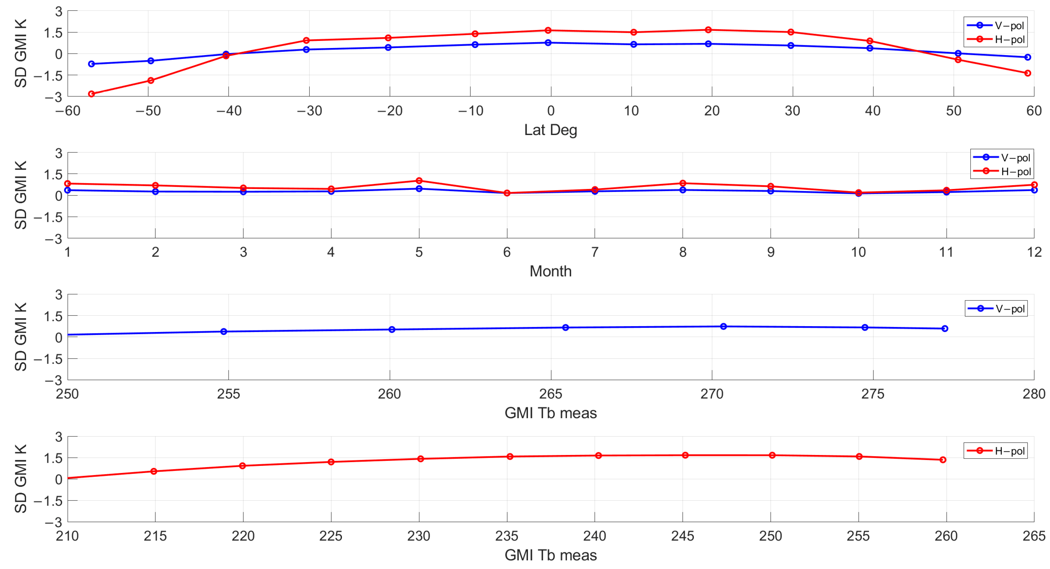
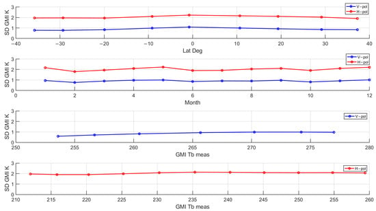
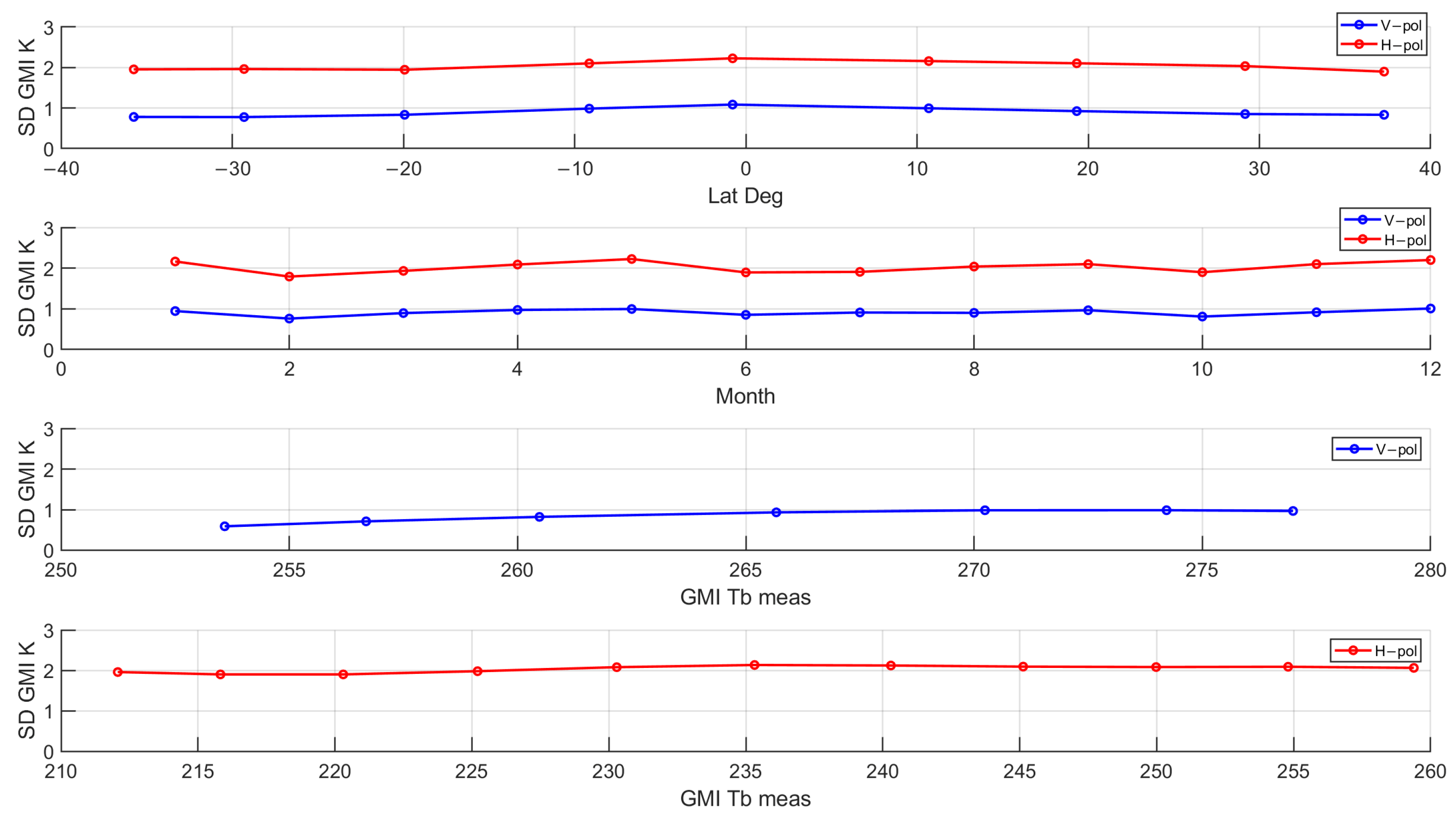
After applying these filters to the preliminary dataset, a systematic variation analysis is performed using the standard XCAL QC filters mentioned above. Specifically, the objective is to demonstrate that the mean GMI SD (measured minus modeled Tb) is constant regardless of how the match-up boxes are sorted and averaged. For example, consider Figure 11, where the mean GMI SDs for the 89 GHz V-pol and H-pol channels are displayed. Here are 4 subplots of SD versus latitude, month of the year, and measured Tb (with V- and H-pol in separate plots). The SD for both polarizations exhibits a pronounced roll-off for latitudes > 30° in both hemispheres, which exceeds our previous experience with cross-track scanners of <1 K. Further, the rate of roll-off is ~6x for H-pol compared to that of V-pol, and based upon these comparisons, these SD results are NOT acceptable for XCAL analysis.
Figure 11.
GMI 89 GHz single difference dependence on latitude, month, and measured Tb for V-pol (blue) and H-pol (red) observations.
On the other hand, SD values binned and averaged versus month are more acceptable, with peak-to-peak variations of 0.3 K for H-pol and 1.2 K for H-pol. Because atmospheric emissions are non-polarized, the stronger H-pol response suggests that the RTM ocean emissivity may be the source of the observed SD variations. Regardless, at this point, there are systematic errors that must be removed before proceeding with the XCAL analysis.
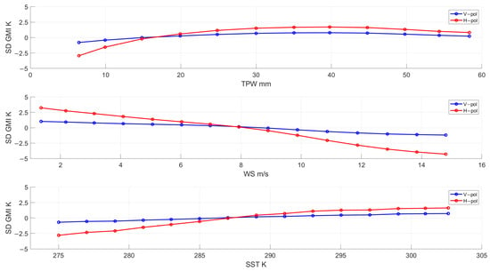
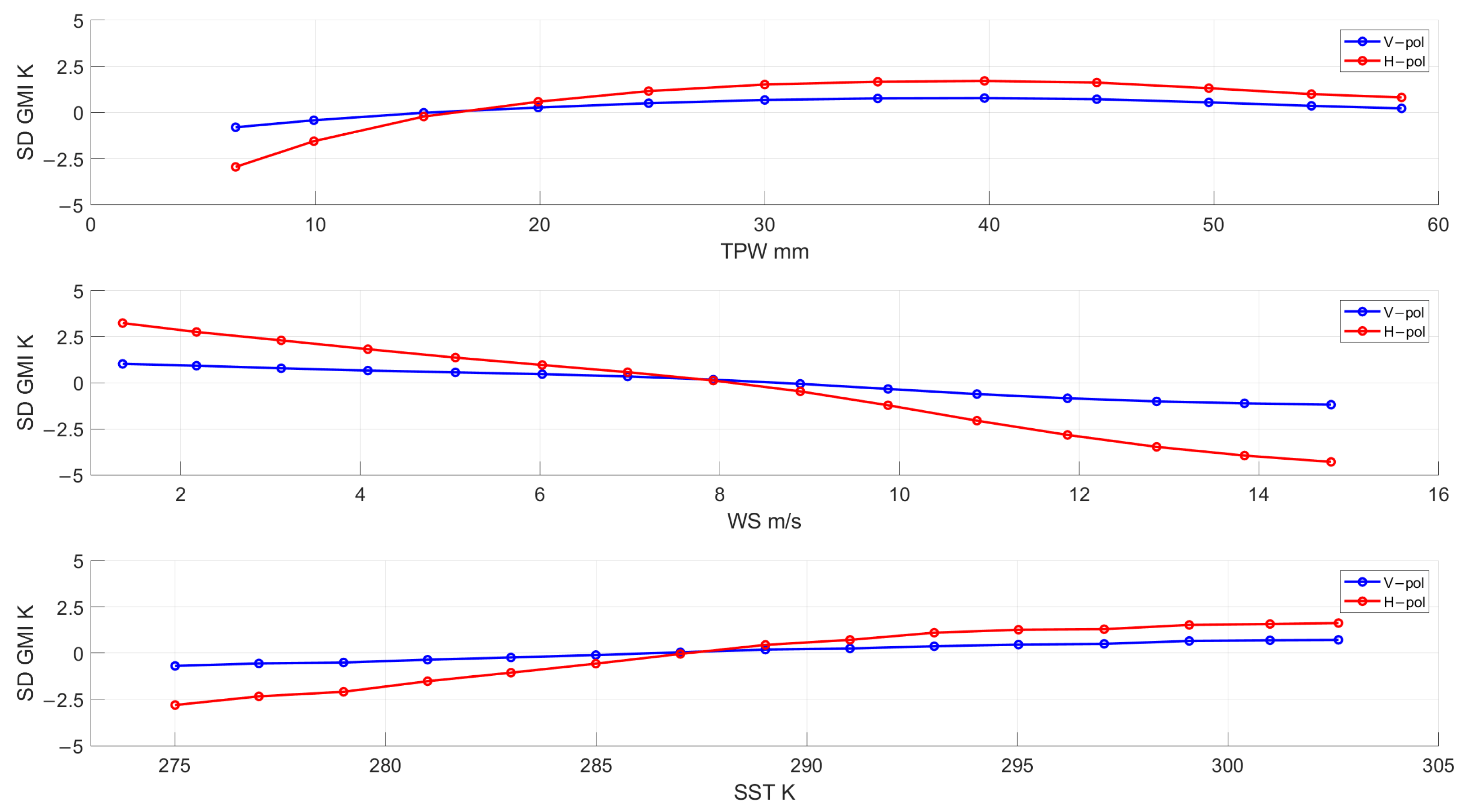
Next, the polarized SDs are sorted by selected environmental parameters in Figure 12. For these comparisons, the H-pol SD exhibits greater changes with total precipitable water (TPW), wind speed, and sea surface temperature (SST) than does the V-pol, which suggests that these environmental conditions may contribute to the observed changes shown in Figure 11. The peak-to-peak variations across TPW, wind speed, and SST were 1.6, 2.2, and 1.4 K for V-pol and 4.6, 7.4, and 4.4 K for H-pol, respectively. These results are a major concern for XCAL, which is discussed in the next section.
Figure 12.
GMI 89 GHz polarized SD dependence on TPW, wind speed, and SST for V-pol (blue) and H-pol (red).
2.4.2. Additional XCAL Data Screening Criteria for GMI 89 GHz
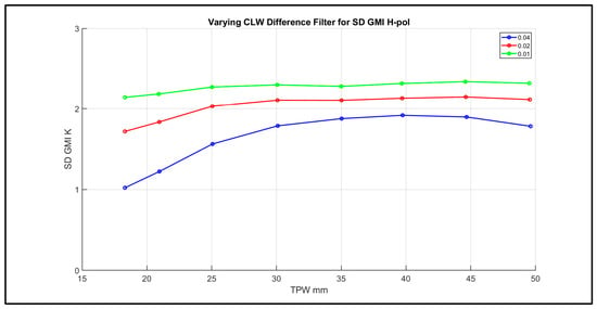
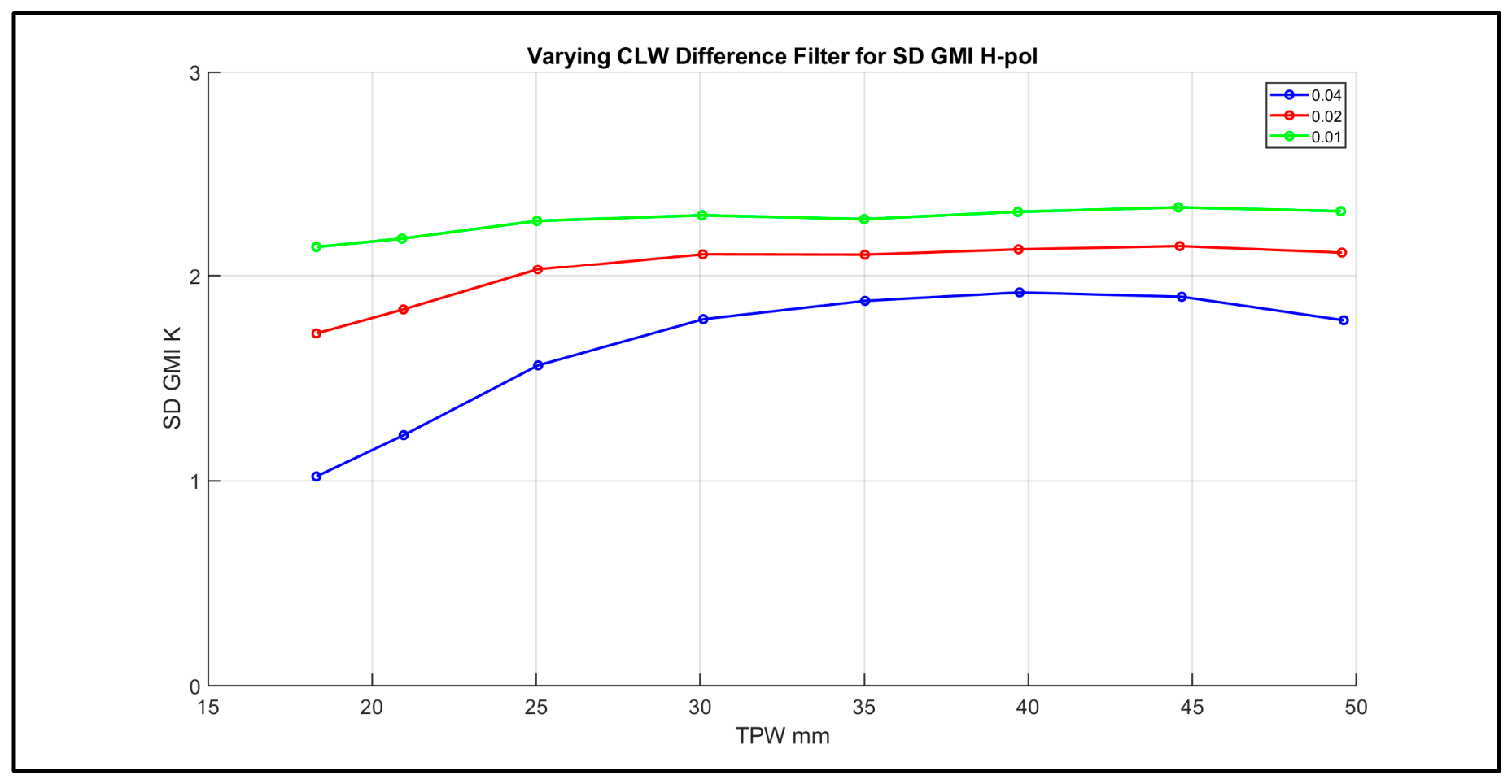
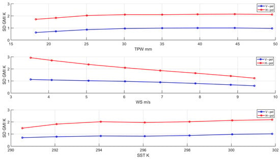
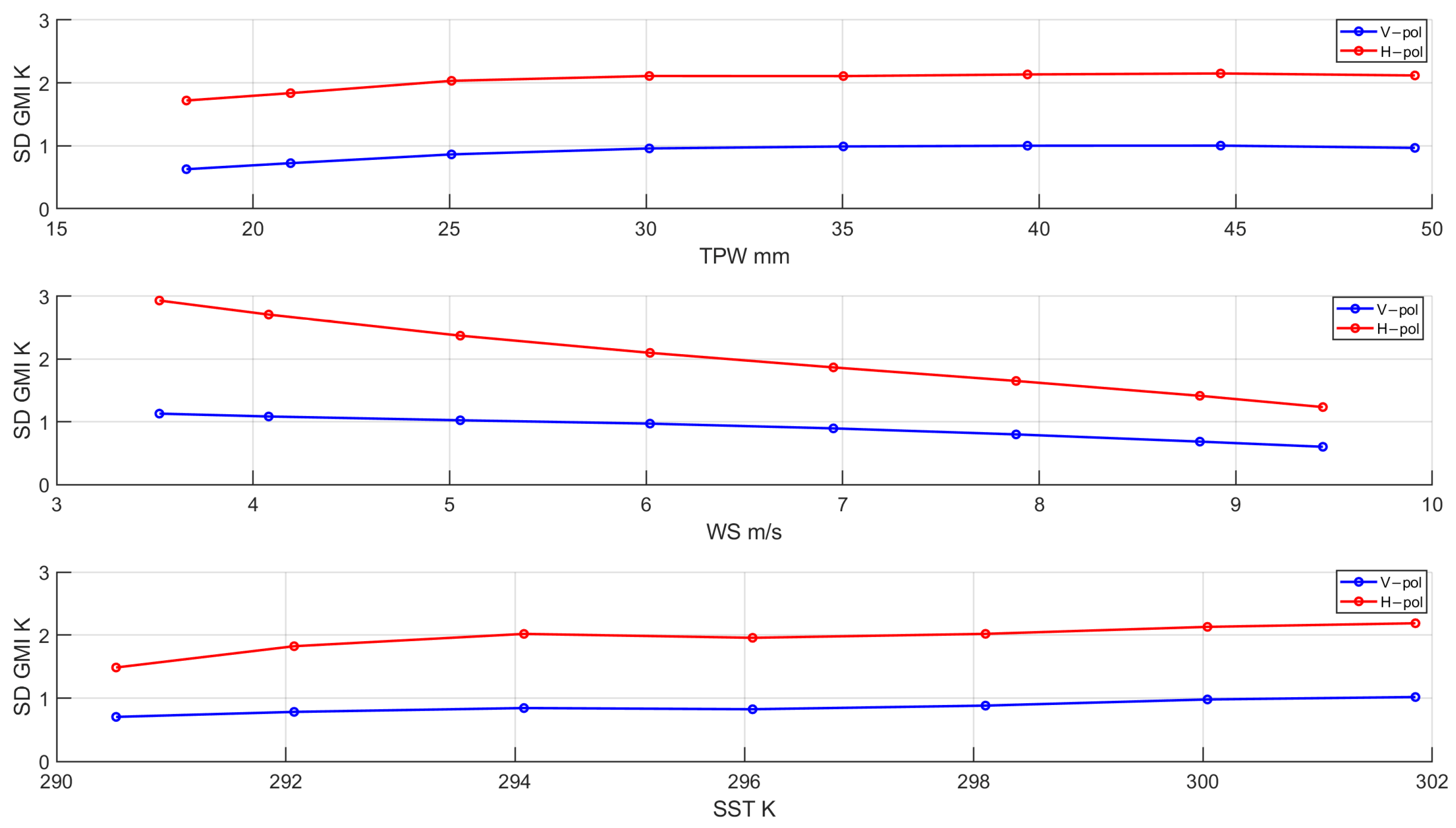
To reduce scene-dependent changes in the GMI SD, additional atmospheric filters were applied to remove boxes where: TPW < 18 mm, apparent cloud ice > 0, and CLW > 0.05 mm. Additionally, ocean environmental parameter QC filters removed boxes where SST < 290 K and surface wind speeds were outside the range of 3 to 10 m/s. Furthermore, to address the sensitivity of the GMI SD to clouds, an additional source for CLW environmental data was introduced into the XCAL analysis. These data were CLW retrievals from GMI brightness temperatures provided by the Remote Sensing Systems (RSS) [13]. Because these retrievals were derived from GMI Tb measurements, they were perfectly aligned in space and time with the GMI measured Tbs; therefore, they could be used to remove conflicting ERA5 CLW data. For each collocated box, the RSS and ERA5 CLW values were compared, and a box was rejected when their absolute difference exceeded a threshold value. A trade study was conducted to establish this filter threshold, and the results are presented in Figure 13 for 3 candidate values. As seen in this figure, the GMI SD is less variable as the threshold decreases, but this was also accompanied by a significant reduction in the number of filtered boxes . So, the compromised 0.02 mm threshold (red curve) was selected, which resulted in a nearly constant SD value for TPW > 25, while retaining more than 1 million collocated matchups over one year.
Figure 13.
GMI 89 GHz H-pol single difference dependence on total precipitable water for varying differential CLW filter thresholds.
Although these new QC filters restrict the range of environmental conditions, their primary effect is to reduce the variability of the GMI SD over a reasonable range of latitudes, while maintaining the maximum possible dynamic range of measured brightness temperatures. After applying the above QC filters, the DD variability is substantially reduced compared with the previous results given in Figure 11. Now, both polarizations exhibit relatively constant SD behavior with respect to the evaluated parameters: latitude, month, and measured brightness temperature (Figure 14). Note that these plots are similar to those given in Figure 11; however, here, the vertical scales are expanded by >3x. The resulting peak-to-peak DD variations across latitude, month, and measured brightness temperature are 0.3, 0.2 and 0.4 K for V-pol, and 0.4, 0.4 and 0.3 K for H-pol, respectively. Furthermore, as seen in Figure 15, the variability of the GMI SD is significantly reduced compared to Figure 12. Now, the new peak-to-peak SD changes with respect to TPW and SST are 0.4 and 0.3 K for V-pol and 0.4 and 0.7 K for H-pol, respectively. However, concerning wind speed, while the changes in SD are reduced, the H-pol gives less than the desired results, with peak-to-peak changes of 1.7 K compared to 0.5 K for V-pol. Nevertheless, these results indicate that the additional screening criteria are successful in reducing the previous scene-dependent variations.
Figure 14.
GMI single SD dependence on latitude, month, and measured brightness temperature after applying more restrictive QC filters. Blue indicates V-pol, and red indicates H-pol observations.
Figure 15.
GMI single-difference dependence on TPW, wind speed, and SST after applying more restrictive QC filters. Blue indicates V-pol, and red indicates H-pol observations.
3. Results
This section presents the results of the GMI XCAL analysis to determine the mean TPX W-band XCAL bias and its uncertainty (bias error). Both values are used when combining Tb measurements, from a constellation of dissimilar MWRs, to produce a unified GPM global rainfall product.
As described in Section 2.2, the most important element of this XCAL process (see Figure 8) is the transform of both Tb measurements to a common basis before comparison. The first step is to combine the GMI 89 GHz linearly polarized Tb to match the mixed polarization of TPX (94.6% H-pol and 5.4% V-pol). Next, the GMI observation, at an incidence angle of 52.8°, is transformed to an equivalent TPX measurement in a cross-track scan at incidence angles between ±70°. Because ocean surface emissivity depends on polarization, incidence angle, and frequency, this produces systematic differences between TPX and GMI Tb observations under identical oceanic and atmospheric environments. These differences are removed using the XCAL MonoRTM to calculate the modeled single difference, which accounts for the respective viewing geometries and channel frequencies in their theoretical Tbs as a function of environmental conditions. Therefore, for a perfectly calibrated constellation MWR, the modeled SD is the expected difference associated with the respective Tb observations. At this point, the target and reference Tbs are equivalent, and the DD is produced by subtracting observed and modeled single differences (OSD—MSD), which is the relative calibration bias.
Our hypothesis is that the calculated DD is a Gaussian-distributed random variable about the true calibration bias, and as such, the mean value must be invariant across all ocean scene observations. Residual DD variations may reflect differences in instrument response (compared with those modeled by RTM), errors in RTM input environmental conditions, or systematic changes in the target MWR Tb transfer function. Therefore, a constant DD result is an important criterion for assessing cross-calibration consistency and the accuracy of the estimated relative radiometric bias.
3.1. GMI Single Difference
As described above, the DD depends on the GMI SD (Figure 10), and we use this as a quality control metric. A Monte Carlo simulation was performed using >40,000 boxes, and the results indicated that a minimum of 2000 boxes yielded a standard deviation in the mean SD of 0.05 K, which is one component of the total error estimate described later. Therefore, in the binned averages presented, the number of independent samples is ≥ 2000.
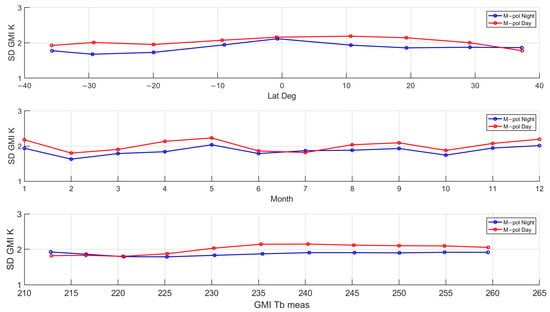
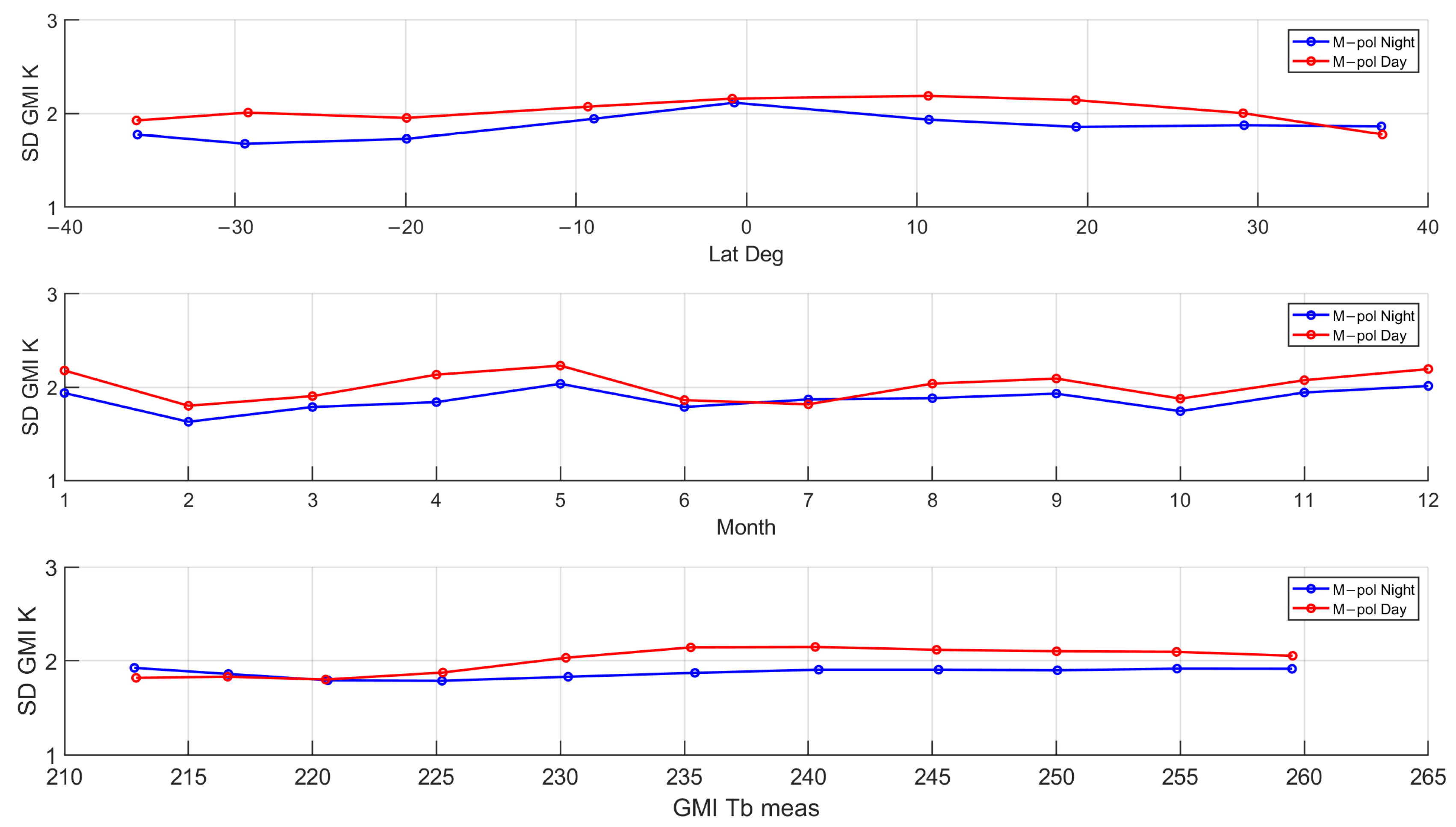
The GMI mixed-polarization SD binned averages (Figure 16) are nearly constant when binned by latitude, month and measured brightness temperature for daytime and nighttime observations. The corresponding peak-to-peak DD variations across latitude, month and measured brightness temperature are 0.47, 0.40 and 0.14 K for nighttime observations and 0.41, 0.34 and 0.32 K for daytime observations, respectively. Note that the mean SD bias is approximately 0.15 K higher during daytime than nighttime observations, indicating a small but consistent day–night difference, the cause of which is unknown.
Figure 16.
GMI 89 GHz mixed-polarization, SD binned averages as a function of latitude, month, and measured brightness temperature. Blue and red indicate nighttime and daytime observations, respectively.
3.2. TPX Single Difference
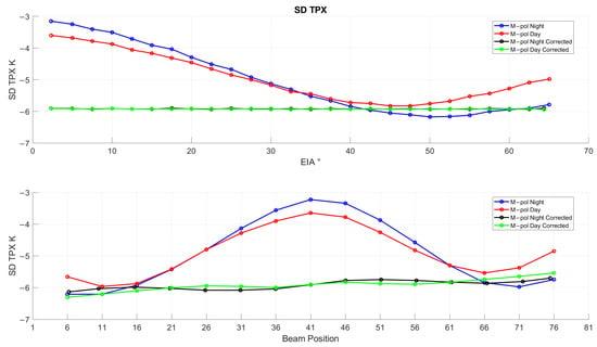
The TPX global mean SD, displayed as a function of EIA (Figure 17, upper panel) for nighttime and daytime orbit segments, has a peak-to-peak variation of 3 K, and because of the TPX cross-track scanning geometry, the EIA is symmetric about beam position 41. Next, the SD is bin-averaged versus beam position, using an averaging window of ±4 beam positions, and these results are shown in the lower panel. Both the observed EIA and beam position dependencies indicate the existence of significant, quasi-sinusoidal changes in the binned-average SD. To remove this effect, an empirical EIA correction is applied. This correction is calculated using the mean TPX SD at the TPX EIA corresponding to the GMI EIA (52.8°). Then, SD values for nighttime and daytime are averaged to define the reference bias, and at each EIA, the difference between the SD and the reference bias is applied as an additive correction to the TPX SD.
Figure 17.
TPX SD dependence on EIA (upper panel) and beam position (lower panel) for nighttime (blue) and daytime (red) observations before and after an empirical SD correction was applied.
After applying this correction, the dependence of the TPX SD on EIA is substantially reduced, as shown by the green and black plots in Figure 17, and the difference between the nighttime and daytime curves is removed. Also, the beam position dependence is similarly reduced; however, the corrected SD retains a modest monotonic increase of approximately 0.7 K over the range of 81 beam positions (lower panel). This residual dependence indicates that the simple EIA correction does not completely remove the beam position dependence.
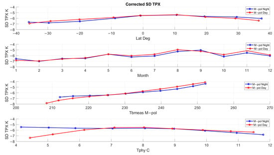
Next, the EIA-corrected TPX SD at beam position 41, was evaluated as a function of latitude, month, measured brightness temperature, and instrument physical temperature for day/night observations (Figure 18). Note that the SD plots are no longer constant, and the peak-to-peak variations across these parameters are 1.0, 1.6, 2.8, and 1.3 K for nighttime observations and 1.2, 1.9, 3.8, and 2.1 K for daytime observations, respectively. Furthermore, the largest variation occurs with measured brightness temperature, which exhibits a strong monotonic increase, and the SD also exhibits a slight seasonal dependence with month, along with differing trends in physical temperature between nighttime and daytime observations. Because these SD variabilities can originate from both the measured and modeled Tb, the root cause cannot be determined using these SD results alone. The observed latitude dependence is associated with the change in brightness temperature across latitude, which is determined by changes in TPW and SST. Regardless of the underlying cause, the observed latitude dependence violates the XCAL requirement that the DD remains independent of the binned parameters. In addition, this analysis was repeated for other beam positions with similar results obtained.
Figure 18.
Dependence of EIA-corrected TPX SD at beam position 41 as a function of latitude, month, measured Tb, and instrument physical temperature. Blue and red indicate nighttime and daytime observations, respectively.
In summary, after applying the simple SD correction for EIA, the TPX SD (Figure 17) appears to satisfy the XCAL hypothesis in that the SD is constant and independent of systematic variations with latitude, month, measured Tb, and physical temperature. However, when sorting the SD observations by beam position (Figure 18), it is apparent that the XCAL bias changes and is no longer constant with these parameters. So, it is concluded that the simple EIA correction does not solve the issue, and therefore, it is disqualified. As a result, the DD comparison results (given next) are without the EIA correction applied. So, this leaves the removal of TPX systematic Tb biases for future work.
3.3. Double Difference
The XCAL DD analysis is performed using the one-year match-ups with improved QC filters (but without the EIA ad hoc correction). The DD data are sorted and binned-averaged as a function of latitude, month, and measured Tb.
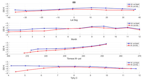
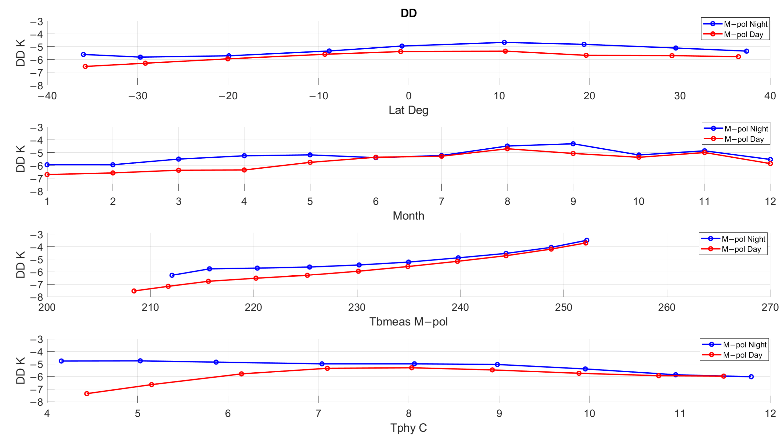
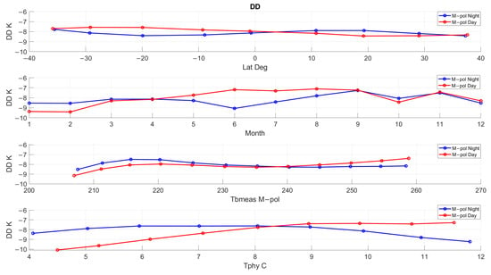
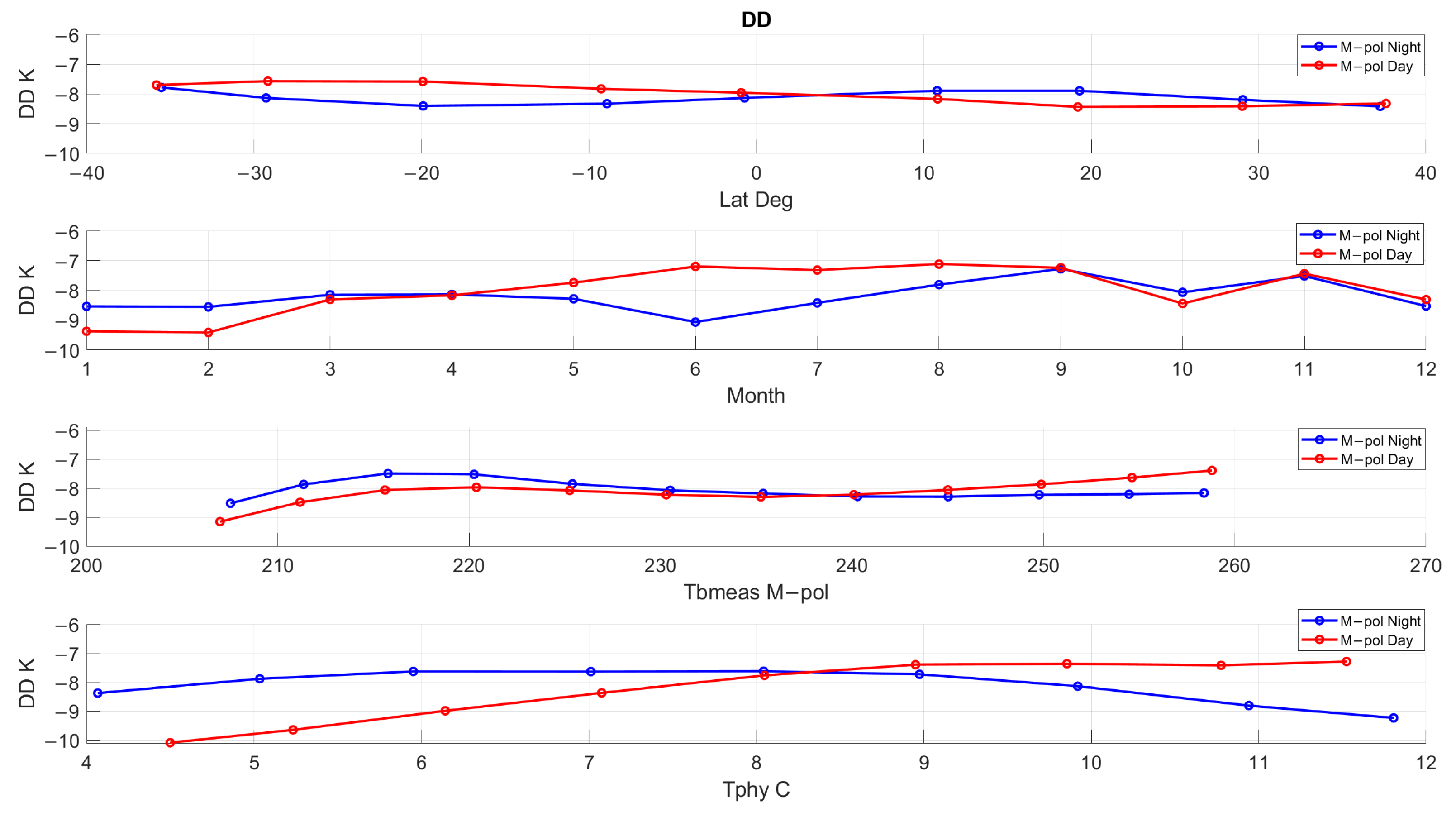
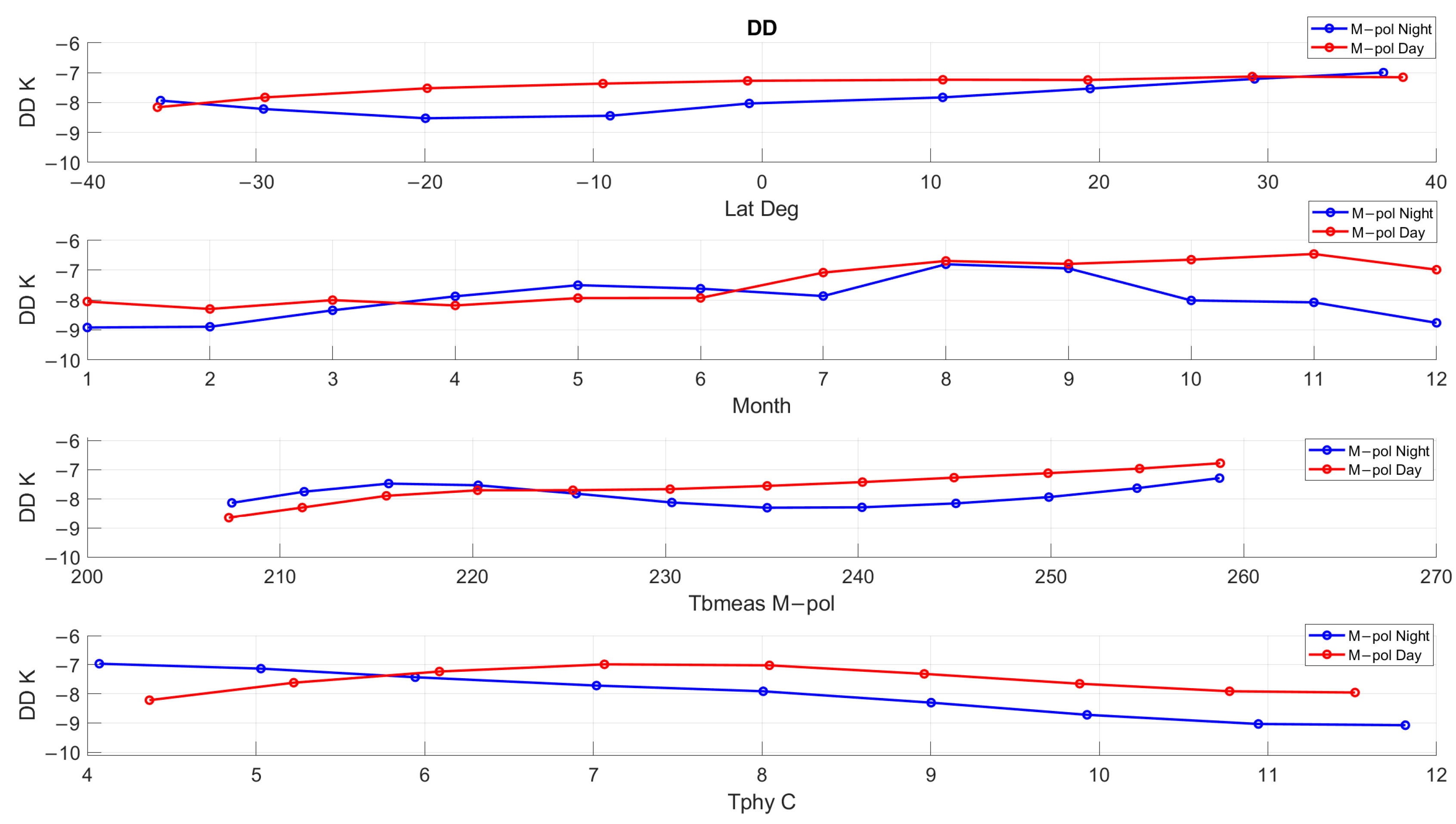
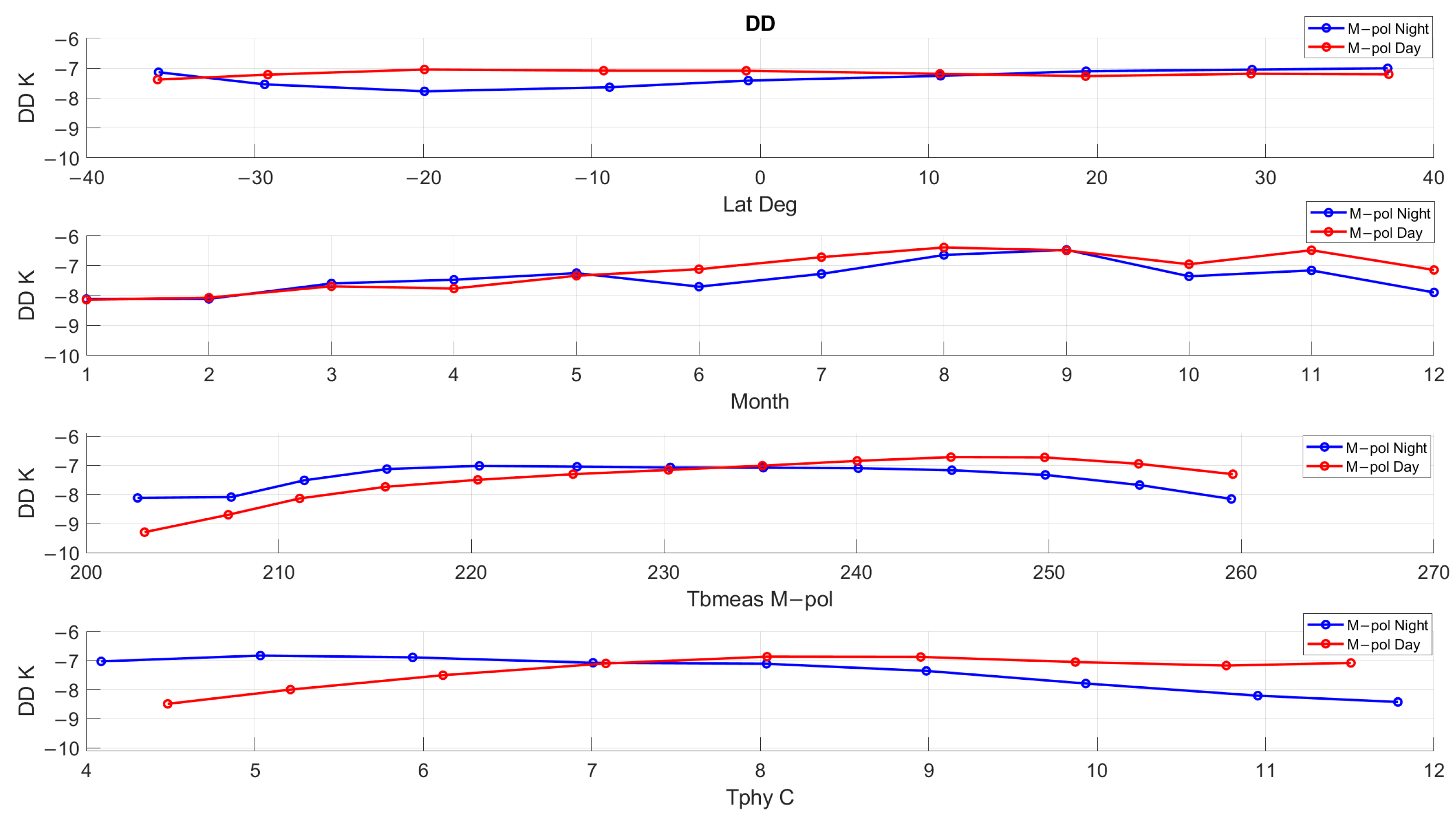
As shown in Figure 19, the resulting DD plots are similar to the corresponding TPX SD plots for both day/night comparisons. These plots exhibit systematic changes with the peak-to-peak DD variations of about 1 K (latitude), 2 K (month), 3 K (Tb measured), and 2 K (instrument physical temperature) for nighttime observations. Note that the greatest DD change occurs with measured brightness temperature, which has a strong monotonic increase. Also, at beam positions 9 and 72 (Figure 20 and Figure 21), the DD plots have patterns similar to those in Figure 19 with respect to all four parameters. Finally, the DD results for all beam positions combined are shown in Figure 22, and the comparisons are very similar to those for the individual beam positions, except that the mean bias values for each differ by a few K.
Figure 19.
Dependence of DD at beam position 41 as a function of latitude, month, measured Tb, and instrument physical temperature. Blue indicates nighttime and red indicates daytime observations.
Figure 20.
Dependence of DD at beam position 9 as a function of latitude, month, measured Tb, and instrument physical temperature. Blue and red indicate nighttime and daytime observations, respectively.
Figure 21.
Dependence of DD at beam position 72 as a function of latitude, month, measured Tb, and instrument physical temperature. Blue and red indicate nighttime and daytime observations, respectively.
Figure 22.
DD all beam positions included as a function of latitude, month, measured brightness temperature, and physical temperature. Blue and red indicate nighttime and daytime observations, respectively.
In summary, when GMI/TPX DD are sorted and bin-averaged by individual beam position, there are systematic variations with latitude, month, measured Tb, and physical temperature that exceed the GPM XCAL 1 K maximum uncertainty limit. However, after applying a simple empirical DD correction versus beam position, the resulting biases are nearly constant within a few tenths of a K uncertainty (results not shown but are essentially identical to Figure 17). On the other hand, when using these same corrected data, the DD comparisons for individual beam positions change considerably by several K, which is in conflict with the previous result for all beam positions combined. Thus, there is some systematic effect in the TPX radiometric calibration that must be removed before the XCAL process can continue, which is the focus of future XCAL investigations.
4. Discussion
This paper describes a robust technique to perform the inter-satellite radiometric calibration (XCAL) between two microwave radiometers of different designs for the Global Precipitation Measurement satellite constellation. For almost two decades, similar comparisons have been performed among microwave radiometers with different scanning geometries, including cross-track scanners [5,9,11], but this paper is the first to perform XCAL with a CubeSat MWR, namely, the TROPICS (TPX) Pathfinder satellite.
The double difference XCAL procedure combines measured and modeled brightness temperatures from both instruments into a common single difference metric before Tb comparison. The SD involves comparing the radiometer measured Tb with a theoretical value from a microwave radiative transfer model. Afterwards, the relative calibration between the target and reference radiometers is achieved by performing a double difference, DD = SDtarget − SDreference. A necessary condition is that both the reference (GPM Microwave Imager) and target (TPX), measured Tb minus modeled Tb, must be a constant value, which is independent of the evaluation approach. For example, when the DD comparisons are sorted and averaged versus latitude, month of year, or Tb measurement, the results must yield the same bias value. If any systematic dependence of the DD value exists, it must be characterized and removed before estimating the calibration bias and its uncertainty.
For the experimental case study, a one-year TPX–GMI matchup dataset is produced by spatially and temporally collocating Tb observations over clear-sky ocean scenes, with corresponding environmental parameters from a numerical weather model. This results in >5 million 0.5° latitude/longitude boxes, of which approximately 1 million remain after final screening for the XCAL DD bias calculation.
The first evaluation uses the GMI 89 GHz channel SD (measured Tb minus modeled Tb) as a quality control filter. The initial XCAL screening showed that GMI SDs exhibited several Kelvin of variability when sorted by latitude, month, measured Tb, and environmental parameters (Figure 11, Figure 12 and Figure 13). Unfortunately, it is not possible to ascertain the source of the variability (measured or modeled Tb), but by restricting the environmental parameter dynamic ranges, it is possible to find an acceptable subset of matchups that produces a nearly constant SD value (see Figure 18). These data are used as the GMI reference for the subsequent XCAL analysis.
The second evaluation characterizes the TPX SD dependence on viewing geometry and other XCAL parameters. As shown in Figure 19, the TPX SD exhibits an unacceptable quasi-sinusoidal dependence on beam position (also EIA). Given this, an empirical TPX SD bias correction (as a function of EIA) is applied, and this results in a constant SD, as shown in the upper panel of Figure 19. However, when evaluated by individual beam positions, the TPX SD is not constant when sorted and averaged by latitude, month, measured Tb and instrument physical temperature.
Next, the GMI/TPX DD is evaluated for systematic dependence on viewing geometry (EIA and beam position), and the results are shown in Figure 21. As expected, for the uncorrected TPX data, there is an unacceptable variable DD dependence on both EIA and beam position, and after applying a TPX SD EIA correction, most comparisons are significantly improved, although a residual monotonic beam-position dependence remains. The EIA correction must be applied to the TPX SD prior to calculating the DD, as systematic dependencies must be removed before proceeding with XCAL. This ensures that the resulting DD remains independent of the binned parameters, satisfying a fundamental requirement of XCAL. Also, there is a small difference (0.15 K) between day and night observations, which is found to be a GMI issue and not attributed to TPX.
Finally, DD values, without the DD correction versus EIA, are examined at fixed TPX beam positions: 41 (mid-swath), 9 and 72 (corresponding to GMI EIA). The results are shown respectively in Figure 19, Figure 20 and Figure 21. For all three beam position cases, there exists a systematic dependence on latitude, month, measured Tb, and physical temperature, which exceeds the maximum allowable uncertainty of the estimated mean DD bias. Furthermore, when all beam positions are combined (Figure 22), these results are not consistent.
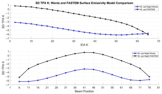
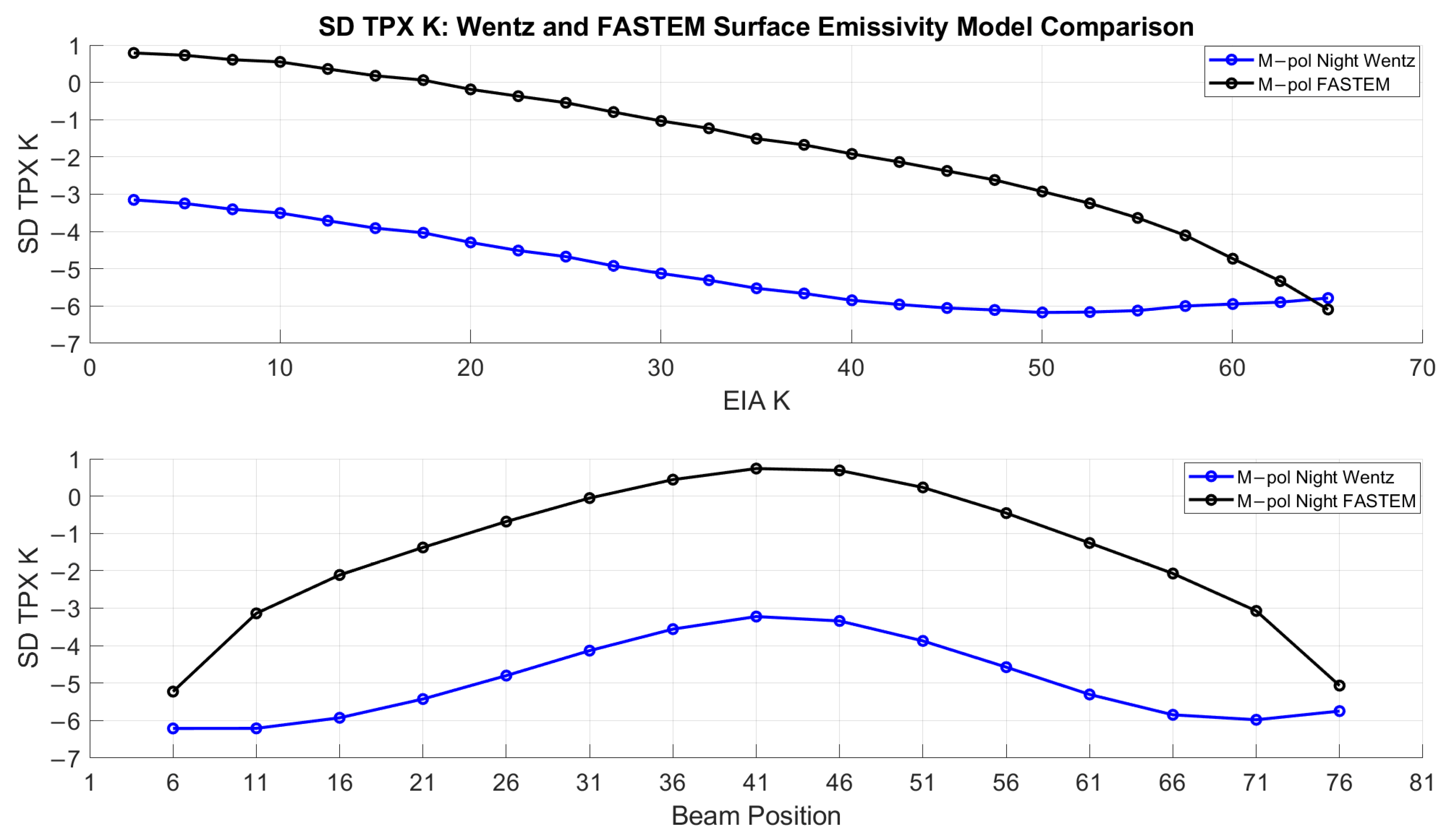
Finally, an investigation was conducted into possible sources of EIA variability in the TPX DD. For this purpose, an alternative surface emissivity model (FASTEM, [14]) was substituted into the XCAL MonoRTM. Both models were used to perform TPX SD (measured—modeled) comparisons, and the results are shown in Figure 23. Although these surface emissivity models produced different bias magnitudes, both exhibited similar trends with respect to modeled Tb versus EIA. The consistency in these trends suggests that the observed incidence angle dependence in the DD bias is not solely attributable to the choice of surface emissivity model. This raises the possibility that other limitations in the RTM representation of incidence angle dependence, particularly in its treatment of atmospheric contributions, may contribute to the observed effects.
Figure 23.
TPX SD dependence on EIA (upper panel) and beam position (lower panel) using two ocean surface emissivity models. Blue represents the SD calculated using the Meissner–Wentz model, and black indicates the FASTEM models.
The change in antenna IFOV for the TPX Tb measurement was also considered a possible cause of the TPX SD incidence angle dependence. From Table 1, the IFOV increases significantly with EIAs between 0° and 65°, and at the GMI incidence angle, the elongated cross-track footprint was 74 km, which was slightly larger than the size of a single box at this incidence angle. However, no apparent evidence was found that suggests that this is a significant factor.
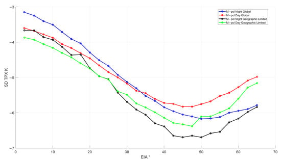
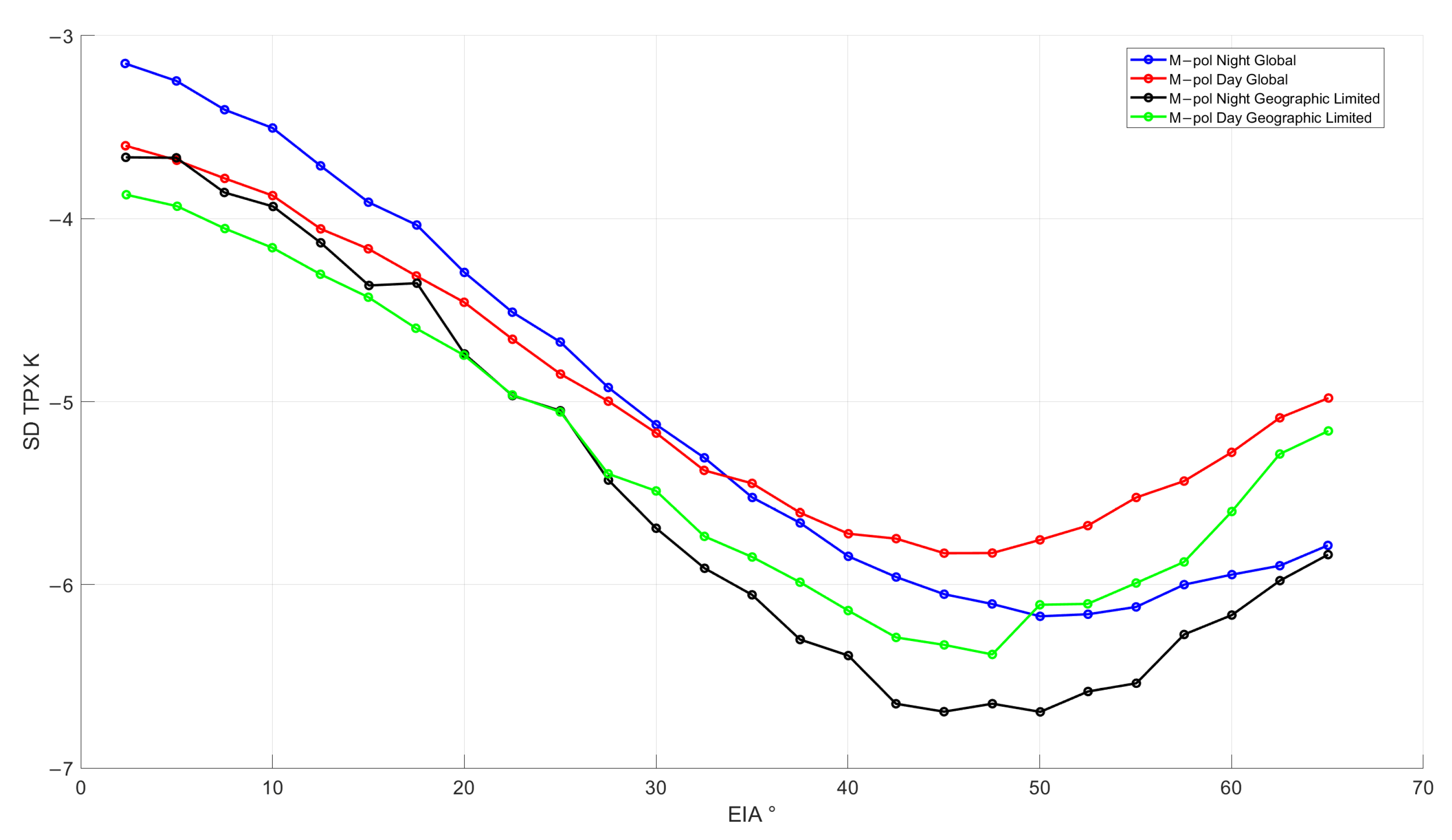
However, the effects of variable antenna beam efficiency (land Tb contamination through antenna sidelobes) were considered a potential cause of the observed change in calibration bias with EIA. For this purpose, day/night comparisons were made between the TPX SD for restricted open ocean SD observations and those of both open and coastal ocean scenes. The results are shown in Figure 24. The similarity of these results strongly suggests that land contamination through antenna sidelobes is not a likely cause.
Figure 24.
TPX SD as a function of EIA for night (blue) and day (red) Tb observations over coastal and open-ocean regions, and Tb observations for a geographically restricted open-ocean region for night (black) and day (green).
Additionally, applying the incidence angle-dependent SD TPX correction only affected the bias magnitude of the SD and DD results when analysis was done by beam position, while the trends between DD and the various XCAL parameters remained unchanged. This indicates that the SD TPX correction was independent of the observed DD dependence on measured brightness temperature and does not account for the trends discussed below.
Interestingly, the DD results at Beam Position 41 (nadir) exhibit a monotonic increase with measured brightness temperature, potentially indicating a nonlinear calibration effect. However, at Beam Positions 9 and 72 (Figure 20 and Figure 21), which correspond to incidence angles matching the GMI viewing geometry, the DD exhibits a relatively flat dependence on measured brightness temperature. This difference in behavior across beam positions suggests that the observed dependence may involve incidence angle-related modeling errors and instrument calibration effects. In particular, the contrasting behavior between nadir and the GMI-matched incidence angles warrants further investigation into the accuracy of the TROPICS calibration across its scan.
5. Conclusions
It is concluded that the relatively constant GMI SD (measured Tb minus modeled Tb), in combination with parameter-dependent changes observed in the TPX SD, suggests that the observed non-constant DD dependence is primarily associated with the TPX contribution. Furthermore, because the current XCAL results cannot distinguish whether this dependence originates from the TPX measured or from the modeled brightness temperatures, additional analysis is required to separate the TPX measurement and modeling contributions. Also, because the current uncertainty in the estimated DD bias exceeds the 1 Kelvin limit, the current match-up dataset does not satisfy the objectives for GMI XCAL. While this XCAL outcome recommends that TPX not join the GPM constellation, it is a success for maintaining the high quality of the GPM global precipitation product.
Further investigations are needed to identify the foot causes of the apparent TPX calibration issues. If no root cause is found, then additional analysis will be conducted using independent TPX–GMI matchups, and even other satellite matchups, to establish statistical correlations between TPX DD anomalies and physical conditions. These analyses could support the development of a physically based calibration approach to address the remaining systematic dependence and improve TPX–GMI cross-calibration. Previous studies have demonstrated successful intercalibration among microwave radiometers with different scanning geometries, including cross-track scanners [5,9,11].
Finally, RTM studies will be performed to validate the XCAL MonoRTM performance under cross-track scanning comparisons, which should improve the XCAL analysis for future CubeSat MWRs.
Author Contributions
All authors contributed to this paper. P.N.D.L.L. performed the XCAL analysis and simulations, and wrote the manuscript. W.L.J. served as the advisor, provided technical expertise and guidance, and contributed to the writing of the manuscript. All authors have read and agreed to the published version of the manuscript.
Funding
This research was funded under grant number 80NSSC25K7998 from NASA Goddard Space Flight Center, titled “Inter-Satellite Radiometric Calibration for TROPICS”.
Data Availability Statement
Data are available on request due to restrictions. The data presented in this study are available upon request from the corresponding author. The processed data supporting the findings of this study are stored on a University of Central Florida (UCF) server and are available upon request. The TROPICS and GMI data used in this study were obtained from the NASA Goddard Earth Sciences Data and Information Services Center (GES DISC), and the RSS data were obtained from Remote Sensing Systems. The ERA5-derived data were obtained through the University of Colorado and are subject to access restrictions. Requests regarding the ERA5-derived data or the processed analysis data should be directed to the corresponding author.
Acknowledgments
We thank NASA Goddard Space Flight Center for providing data, funding, and support. GMI data are produced by Remote Sensing Systems and sponsored by NASA Earth Science funding. Data are available at www.remss.com, accessed on 12 November 2026.
Conflicts of Interest
The authors declare no conflicts of interest.
References
- Draper, D.W.; Newell, D.A.; Wentz, F.J.; Krimchansky, S.; Skofronick-Jackson, G. The Global Precipitation Measurement (GPM) Microwave Imager (GMI): Instrument Overview and Early On-Orbit Performance. IEEE J. Sel. Top. Appl. Earth Obs. Remote Sens. 2015, 8, 3452–3462. [Google Scholar] [CrossRef] [Scilit]
- Huffman, G.J.; Bolvin, D.T.; Joyce, R.; Nelkin, E.J.; Tan, J.; Braithwaite, D.; Hsu, K.; Kelley, O.A.; Nguyen, P.; Sorooshian, S.; et al. NASA Global Precipitation Measurement (GPM) Integrated Multi-Satellite Retrievals for GPM (IMERG) Version 07: Algorithm Theoretical Basis Document (ATBD); NASA: Greenbelt, MD, USA, 2023.
- Huffman, G.J.; Bolvin, D.T.; Braithwaite, D.; Hsu, K.; Joyce, R.; Kidd, C.; Nelkin, E.J.; Sorooshian, S.; Stocker, E.F.; Tan, J.; et al. Integrated Multi-satellite Retrievals for the Global Precipitation Measurement (GPM) Mission (IMERG). In Satellite Precipitation Measurement; Levizzani, V., Kidd, C., Kirschbaum, D., Kummerow, C., Nakamura, K., Turk, F., Eds.; Springer: Cham, Switzerland, 2020; Volume 67, pp. 343–353. [Google Scholar] [CrossRef] [Scilit]
- Biswas, S.K.; Farrar, S.; Gopalan, K.; Santos-Garcia, A.; Jones, W.L.; Bilanow, S. Intercalibration of Microwave Radiometer Brightness Temperatures for the Global Precipitation Measurement Mission. IEEE Trans. Geosci. Remote Sens. 2013, 51, 1465–1477. [Google Scholar] [CrossRef] [Scilit]
- Berg, W.; Bilanow, S.; Chen, R.; Datta, S.; Draper, D.; Ebrahimi, H.; Farrar, S.; Jones, W.L.; Kroodsma, R.; McKague, D.; et al. Intercalibration of the GPM Microwave Radiometer Constellation. J. Atmos. Ocean. Technol. 2016, 33, 2639–2654. [Google Scholar] [CrossRef] [Scilit]
- Chen, R.; Ebrahimi, H.; Jones, W.L. Creating a Multidecadal Ocean Microwave Brightness Dataset: Three-Way Intersatellite Radiometric Calibration among GMI, TMI and WindSat. IEEE J. Sel. Top. Appl. Earth Obs. Remote Sens. 2017, 10, 2623–2630. [Google Scholar] [CrossRef] [Scilit]
- Chen, R.; Alquaied, F.; Jones, W.L. Assessing Radiometric Stability of the 17-Plus-Year TRMM Microwave Imager 1B11 Version-8 (GPM05) Brightness Temperature Product. Climate 2017, 5, 92. [Google Scholar] [CrossRef] [Scilit]
- Chen, R.; Jones, W.L. Creating a Consistent Multi-Decadal Oceanic TRMM-GPM Brightness Temperature Record with Estimated Calibration Uncertainty. Climate 2020, 8, 31. [Google Scholar] [CrossRef] [Scilit]
- Ebrahimi, H.; Chen, R.; Jones, W.L. Calibration of Millimeter Wave Sounder Radiometers on Polar Orbiting Satellites. IEEE J. Sel. Top. Appl. Earth Obs. Remote Sens. 2017, 10, 2849–2854. [Google Scholar] [CrossRef] [Scilit]
- Ebrahimi, H.; Datta, S.; Jones, W.L. Intercalibration of Cross-Track Scanners in GPM Constellation. IEEE Trans. Geosci. Remote Sens. 2018, 56, 5749–5757. [Google Scholar] [CrossRef]
- De La Llana, P.N.; Kashem, F.B.; Jones, W.L. Use of Radiative Transfer Model for Inter-Satellite Microwave Radiometer Calibration. Remote Sens. 2025, 17, 1519. [Google Scholar] [CrossRef] [Scilit]
- Meissner, T.; Wentz, F.J. The Emissivity of the Ocean Surface between 6 and 90 GHz over a Large Range of Wind Speeds and Earth Incidence Angles. IEEE Trans. Geosci. Remote Sens. 2012, 50, 3004–3026. [Google Scholar] [CrossRef] [Scilit]
- Wentz, F.J.; Meissner, T.; Scott, J.; Hilburn, K.A. Remote Sensing Systems GPM GMI Daily Environmental Suite on 0.25° Grid, Version 8.2; Remote Sensing Systems: Santa Rosa, CA, USA, 2015; Available online: https://www.remss.com/missions/gmi/ (accessed on 30 September 2026).
- Liu, Q.; Weng, F.; English, S.J. An Improved Fast Microwave Water Emissivity Model. IEEE Trans. Geosci. Remote Sens. 2011, 49, 1238–1250. [Google Scholar] [CrossRef] [Scilit]

Disclaimer/Publisher’s Note: The statements, opinions and data contained in all publications are solely those of the individual author(s) and contributor(s) and not of MDPI and/or the editor(s). MDPI and/or the editor(s) disclaim responsibility for any injury to people or property resulting from any ideas, methods, instructions or products referred to in the content. |
© 2026 by the authors. Licensee MDPI, Basel, Switzerland. This article is an open access article distributed under the terms and conditions of the Creative Commons Attribution (CC BY) license.