


Highlights
What are the main findings?
- •
- TROPOMI SIF and MODIS/Aqua NDVI provided complementary but non-equivalent evidence of cyclone-associated vegetation responses.
- •
- Among 12 study areas (nested within seven cyclones), photosynthesis-linked SIF decreased while canopy greenness increased in three study areas.
What are the implications of the main findings?
- •
- Vegetation responses to tropical cyclones cannot be inferred reliably from canopy greenness alone.
- •
- Explicit reporting of sampling support and spatial uncertainty is essential when interpreting event-level SIF responses.
Abstract
Satellite assessments of vegetation responses to tropical cyclones depend on both indicator sensitivity and observational availability. We evaluated 21 storm-country study areas in Southern Africa from 2018 to 2021 using TROPOspheric Monitoring Instrument (TROPOMI) solar-induced chlorophyll fluorescence (SIF) as a photosynthesis-linked indicator and Aqua Moderate Resolution Imaging Spectroradiometer (MODIS) normalised difference vegetation index (NDVI) as an independent measure of canopy greenness. Storm-week responses within 200 km of cyclone tracks were estimated using spatial-block bootstrap intervals. Usable storm-week SIF was available for 12 study areas (nested within seven cyclones), whereas NDVI was available for all 21. Across the 12 matched study areas, SIF changes ranged from −42.9% to +35.5% and NDVI changes from −4.0% to +6.1%. The +35.5% Desmond extreme represents storm-week SIF remaining above the pre-storm baseline while a pre-existing greening trajectory was interrupted, not cyclone-enhanced photosynthesis; the −42.9% Chalane–Zimbabwe extreme is based on two usable SIF days and is interpreted cautiously. At the study-area level, the indicators agreed in two cases, opposed one another in three, and were statistically unresolved in seven because at least one interval included zero; these 2/3/7 counts do not represent independent cyclone events. Diane, Francisco, and Kenneth showed SIF decreases alongside NDVI increases, demonstrating that greenness did not reproduce the direction of the photosynthesis-linked response. NDVI generally returned to its seasonal range earlier than SIF. These findings show that SIF and NDVI provide complementary but non-equivalent evidence and that sparse SIF sampling determines which cyclone responses can be distinguished from no change.
1. Introduction
Tropical cyclones are among the most disruptive hydroclimatic hazards in Southern Africa, particularly along the eastern seaboard and the inland corridors behind it [1]. Madagascar and Mozambique experience the most frequent landfalls [2], while storm tracks can carry damaging wind and rainfall into Zimbabwe, Zambia and Malawi [3]. Recent records also indicate shifts in the timing and latitude of regional cyclone activity [4]. Consistent satellite observations are therefore needed to compare vegetation conditions across storms, countries and stages of post-storm recovery.
Cyclone formation and intensification in the region are governed largely by the thermal state of the southwest Indian Ocean [2]. Warm sea-surface temperatures increase atmospheric instability and support storm development toward landfall [5]. Climate modes further alter these conditions; during La Niña, moisture transport from the western Indian Ocean can favour cyclone formation and inland penetration [5]. Interannual rainfall variability is strongly influenced by the El Niño–Southern Oscillation, with drier conditions during El Niño phases and wetter conditions during La Niña, and an intensifying long-term drought regime has been identified across much of the subcontinent [1,5,6]. Because these systems usually arrive during the rainy season, their rainfall can fall on already-wet catchments and amplify runoff, flooding and waterlogging.
Rural livelihoods and rainfed agriculture across Southern Africa are closely connected to vegetation condition [7]. Cyclones can damage crops through wind, waterlogging and foliage loss, while surviving vegetation may also experience reduced photosynthetic activity. Stomatal closure, chlorophyll degradation and loss in leaf area can reduce carbon uptake during tissue repair [8]. The vegetation at risk ranges from miombo woodland across Zambia, Zimbabwe and central Mozambique to savanna, bushveld, semi-arid shrubland, grassland and the humid forests of Madagascar, and these ecosystems differ in their sensitivity to water availability [9,10], so one storm need not affect them alike. However, the magnitude and direction of the observed response depend on storm exposure, antecedent ecosystem conditions and the indicator used to measure vegetation change.
Mozambique is among the most cyclone-exposed countries in Africa, and cyclones Idai, Chalane and Eloise made landfall near Beira and reached inland into Zimbabwe and Malawi within a 26-month period, damaging settlements, agriculture and infrastructure [3,11,12]. Households with limited insurance, market access and adaptive capacity are especially vulnerable to these disturbances, and the region’s dependence on rainfed small-scale agriculture links such events to food security, public health, biodiversity and national economic growth across Southern African Development Community (SADC) countries [13,14,15,16]. Vegetation responses also vary with antecedent moisture conditions. Cyclone rainfall may relieve water limitation in semi-arid systems, whereas wind, flooding and waterlogging may suppress vegetation functioning in wetter environments [14,17]. Because cyclones commonly arrive near the peak of the wet season, rainfall may fall on already saturated soils, so antecedent soil moisture strongly determines whether a storm supplies a water subsidy or causes waterlogging and physiological stress [18]. Meteorological records alone therefore cannot determine the vegetation response, and field observations are rarely available across the full storm corridor; monitoring is further constrained by persistent cloud cover and limited regional data [19].
Remote sensing provides spatially consistent observations where field measurements are sparse. Most regional vegetation assessments have used the normalised difference vegetation index NDVI [10], a well-established measure of canopy greenness and cover [20]. Solar-induced chlorophyll fluorescence (SIF), in contrast, is linked to absorbed light and photosynthetic functioning [21,22,23], and reported associations between SIF and productivity loss, together with its use in in-season yield prediction, make it a useful addition to reflectance indices for assessing vegetation disruption and recovery [24,25]. SIF and NDVI therefore represent related but non-equivalent canopy properties. Their responses may agree, oppose one another or remain indeterminate when sampling uncertainty is large.
Satellite assessments of cyclone effects on vegetation remain dominated by case studies of individual storms. Multi-temporal Landsat and Sentinel imagery has been used to map the footprint of Cyclone Idai over Mozambique [26,27], and comparable multispectral analyses exist for Hurricane Maria over Dominica and Puerto Rico [28] and for Cyclone Sidr over the Sundarbans [29]. Earlier work used the Moderate Resolution Imaging Spectroradiometer (MODIS) enhanced vegetation index to identify hurricane disturbance along the northern Gulf of Mexico [30], and satellite data have also been used to contrast the imprint of individual storms within the Mozambique Channel [31]. These studies establish that cyclones leave a detectable optical signature, but they rest almost entirely on reflectance-based greenness indices, they typically report a single event, and they seldom state whether the available sampling was sufficient to detect the response they describe.
The TROPOspheric Monitoring Instrument (TROPOMI) on Sentinel-5P provides spatially explicit SIF observations suitable for regional event analysis [32]. Alternative global SIF records are generated by neural-network reconstruction and by machine-learning gap filling rather than by direct retrieval [33,34], so the choice among them is a choice about what the fluorescence record represents. However, cyclone monitoring presents an observability problem. Cloud screening, irregular usable retrievals and the short duration of storm-response windows can leave some events with only one or two usable SIF days, while MODIS NDVI offers a different temporal support and measurement sensitivity. A comparison of the two indicators must therefore distinguish biological disagreement from unequal availability and statistical uncertainty.
Existing regional evidence is dominated by individual cyclones, particularly Idai, and often aggregates responses over national territories [26,31]. Country-wide averaging can dilute local signals because cyclone tracks intersect only part of a country. More importantly, previous applications have seldom reported whether satellite sampling was sufficient to determine an event-level response or whether apparent SIF–greenness differences exceeded their spatial uncertainty. This observability gap limits comparison across storms and complicates interpretation of post-event return toward seasonal conditions.
This paper evaluates how far cyclone-associated vegetation responses can be observed for 21 storm-country events in Southern Africa. We address three questions: (i) which events have sufficient storm-week SIF observations for quantitative analysis; (ii) when do the directions of SIF and MODIS/Aqua NDVI responses agree, disagree or remain uncertain after spatial uncertainty is considered; and (iii) how do observational availability and spatial dependence constrain interpretation of storm-week and post-storm conditions? SIF is the primary photosynthesis-linked indicator, while NDVI provides an independent greenness comparison. The near-infrared radiance of vegetation (NIRvR) and apparent fluorescence yield (ΦF) provide supporting diagnostics of the observed SIF response, and Penman–Monteith–Leuning version 2 (PML-V2) gross primary production (GPP) provides an exploratory product comparison where available, and rainfall and track proximity provide exploratory environmental context. The contribution is an uncertainty-aware event framework that separates the responses the satellite record can support from those it cannot and states the conditions under which an event-level conclusion is not available.
2. Materials and Methods
2.1. Study Area, Cyclone Events and Datasets
The study domain covers the Southern African subcontinent within the SADC boundary (Figure 1), extending approximately from 10°E to 50°E and 35°S to 5°N, encompassing mainland southeastern Africa and Madagascar. It represents the principal landfall and inland transit corridor of the southwest Indian Ocean tropical cyclones, most directly affecting Mozambique and Madagascar, and sometimes extending into Zimbabwe and neighbouring countries. The region spans strong climatic and topographic gradients, from the humid eastern escarpment of Madagascar and the Mozambican coastal plain to the 1000–1500 m interior plateau and the arid Kalahari margins. These gradients shape cyclone rainfall, hydrological response and vegetation sensitivity.
Figure 1.
Location of the Southern African study domain and study countries. The inset locates the domain within Africa.
Tropical savanna (Aw) and hot semi-arid (BSh) climates dominate the domain, with hot deserts in the southwest [35]. Vegetation ranges from miombo woodland across Zambia, Zimbabwe and central Mozambique to savanna, bushveld, semi-arid shrubland, grassland and the humid forests of Madagascar [36]. Regional hydrology is organised around the transboundary Zambezi, Limpopo, Save and Pungwe basins, which drain eastwards through the main landfall corridor [37]. The standardised 200 km corridor used throughout is an analytical domain rather than a physical impact boundary, as Section 2.2 explains.
This study evaluates cyclone-associated changes in vegetation photosynthetic activity across Southern Africa using an event-based framework for 2018–2021. The overall analytical workflow is summarised in Figure 2. TROPOMI SIF is the primary functional indicator, MODIS/Aqua NDVI provides an independent canopy-greenness comparison, and PML-V2 GPP provides an exploratory cross-product comparison. NIRvR and ΦF are used to interpret the observed SIF response rather than as independent validation measurements. Storm-week responses are the principal outcome; post-event trajectories are evaluated only where usable observations exist. The leave-one-year-out short multi-year seasonal reference controls seasonal timing but is not a contemporaneous untreated control.
Figure 2.
Analytical workflow for assessing cyclone-associated photosynthetic change across Southern Africa.
Event definition proceeded in three stages. The complete event-inclusion and SIF-observability rules are listed in Table 1. First, meteorological and exposure criteria identified 21 storm-country events. Second, the local TROPOSIF (TROPOMI solar-induced fluorescence) Level-2B holding provided storm-week source files for 12 events. Ava and Eliakim over Madagascar precede the TROPOSIF v2.1 record, which begins on 1 May 2018. The other seven events fall between January and March 2021, whereas the 2021 files in the local holding used for the response analysis begin on 25 April 2021. A subsequent provider-archive audit confirmed that daily TROPOSIF files exist within all seven storm windows: two of seven days for each study area affected by Eloise, four of seven for Guambe over Mozambique and six of seven for Iman over Madagascar (Table S1). These files were not part of the response analysis reported here, so quantitative SIF analysis remains restricted to the original 12 events and the seven 2021 cases are identified as local-ingestion exclusions rather than satellite non-observations. Third, the existing quality control (QC), including the cloud-fraction threshold, determined which soundings were usable for the 12 analysed events. The analytical unit is the storm-country event, defined by a cyclone track intersecting a national boundary. Because one cyclone can intersect several countries, these events are not independent replicates: the 12 analysed study areas comprise seven cyclones, with Chalane contributing four study areas and Idai three. Weak or remnant in-country circulation is described as rainfall/flood exposure rather than assumed to represent an intense-wind landfall.
Table 1.
Event inclusion and SIF-observability criteria. Event inclusion defines the 21 storm-country study areas; SIF observability determines the 12 study areas entering the quantitative storm-week SIF analysis.
Cyclone track data come from the International Best Track Archive for Climate Stewardship IBTrACS [38], which records the 6-hourly position, maximum sustained wind speed and minimum central pressure for every cyclone. Event-level exposure was summarised by the maximum World Meteorological Organization (WMO)-reported 10 min wind on the anchor calendar date, converted from knots to kilometres per hour, and by Climate Hazards Group InfraRed Precipitation with Station data CHIRPS [39] rainfall totals over the 60-day antecedent period (days −74 to −15) and storm week (days 0 to +6). Rainfall is reported as the median and interquartile range across the event study-area grid cells (Table S1). These quantities characterise the environmental setting and are not treated as a causal dose. The primary functional indicator is SIF from TROPOMI on Sentinel-5P, taken from the TROPOSIF Level-2B product at 743 nm (SIF_Corr_743, mW m−2 sr−1 nm−1) [32]. TROPOMI provides near-daily global coverage with a nadir footprint of 3.5 by 7 km before 6 August 2019 and 3.5 by 5.5 km thereafter, following an along-track resolution upgrade, with the footprint widening across-track toward the swath edges. Cyclone Idai (March 2019) was therefore observed at the coarser 3.5 by 7 km footprint, while Chalane (December 2020) and Eloise (January 2021) were observed at 3.5 by 5.5 km. Retrievals were retained when cloud fraction was below 0.02, solar zenith angle was below 85 degrees, and top-of-atmosphere radiance was between 20 and 200 mW m−2 sr−1 nm−1. TROPOMI acquires SIF near 13:30 local solar time; the distributed TROPOSIF Level-2B product already includes the published daily correction described in Köhler et al. [40]. Comparison with independently generated PML-V2 GPP is treated as exploratory and descriptive. As an observation-support sensitivity check, relaxing the cloud-fraction threshold from 0.02 to 0.05, while retaining all other filters added 641 storm-week soundings across the 12 analysed study areas but added no usable storm-week day (Table S2). The primary 0.02 estimates were retained because the complete climatological-reference and block-bootstrap analysis was not rerun at 0.05.
Gross primary production is the PML-V2 product, Earth Engine collection CAS/IGSNRR/PML/V2_v018, distributed as 8-day composites at 500 m, covering 26 February 2000 to 27 December 2023, so the 2018–2021 study period lies well inside its record [41]. Its GPP band is a daily mean rate in grams of carbon per square metre per day rather than an 8-day total, so no division by the composite interval is applied; over the Zimbabwe Idai study area the composite beginning 6 March 2019 has a median of 6.8 g of carbon per square metre per day. Only correlations of paired anomalies are reported, and correlation is invariant to constant scaling. GPP is compared with SIF, a carbon flux product generated independently of the TROPOMI retrieval. Correlations based on as few as three paired composites are descriptive and highly uncertain. Ecosystem stratification follows the Ecoregions2017 biome map [36]. National boundaries are from the Database of Global Administrative Areas [42]. EPSG:4326 was used for geographic extraction. Footprint and national areas were computed in a Lambert Azimuthal Equal-Area projection centred on each event’s study-area centroid (World Geodetic System 1984, WGS84 datum), so that the 200 km buffer distance and the derived areas are both metrically correct at the latitude of each event. National areas obtained from the dissolved Ecoregions2017 polygons agree with published land areas to within 1% for Zimbabwe, Botswana, Madagascar and South Africa, and to 3.8% for Mozambique, where the ecoregion coverage omits part of the coastal margin.
2.2. Spatial Framework, SIF Processing and Event-Response Calculation
The analysis avoids country-level aggregation and evaluates cyclone-associated anomalies at the satellite-footprint scale. For the principal analysis, each IBTrACS track was represented as a LineString and buffered by a standardised 200 km radius to provide a common analytical domain across events. The 200 km radius was selected as a standardised compromise: it is wide enough to include near-track vegetation potentially affected by spatially displaced wind and rainfall, while limiting dilution by more distant land and retaining an identical domain definition across storms. This fixed-radius corridor is not interpreted as the physical wind, rainfall or ecological impact boundary of every cyclone. Sensitivity was evaluated at 100, 150, 200 and 300 km; these alternatives show how the estimated response depends on spatial scale rather than establishing that any radius is physically superior. The resulting analytical corridor defines the spatial domain of analysis. Coverage diagnostics quantify the limitations of national aggregation. The coverage fraction (CF) and dilution factor (DF) are defined as:
where Afp is the storm study-area extent and Ac is national area. CF is a geometric coverage fraction and is a potential geometric dilution factor. Interpreting DF as signal dilution assumes that the cyclone-associated anomaly is concentrated inside the study area and negligible outside it; no national sign reversal is inferred without direct country-wide calculations. These diagnostics are not analytical variables in the SIF or GPP calculations.
TROPOMI SIF retrievals were processed for each storm-country event following the quality-control procedure in Section 2.1. Non-vegetated and open-water soundings were removed using a threshold greater than 0.10 on the TROPOMI-derived NDVI, computed from the 665 and 781 nm top-of-atmosphere reflectances; this NDVI is a component of NIRvR only and is distinct from the independent MODIS/Aqua NDVI compared in Section 2.3. Retained retrievals were aggregated to daily estimates and used to decompose SIF into its NIRvR–ΦF terms as described below. Instantaneous SIF depends on solar geometry, so it is normally converted to a daily equivalent. Following Köhler et al. [40], the TROPOSIF Level-2B product distributes SIF_Corr_743 with the daily correction already applied. The analysis therefore used SIF_Corr_743 directly without reapplying the correction. Equations (3) and (4) document the published correction only.
where the Daily Correction Factor is:
where θ denotes the solar zenith angle and H restricts integration to daylight hours. This transformation yields temporally consistent estimates comparable across events. Across all observations in this study, the mean day-length correction factor (DCF) was 0.353, with a range of 0.28 to 0.42 and a standard deviation of 0.031, reflecting the expected seasonal variation in solar geometry across the austral summer study period. Daily values were aggregated to a 0.1° grid by mean compositing of QC-passing soundings (a minimum of two soundings per grid cell). Event- and window-level study-area means reported in the tables are equal-weighted means of available daily study-area means; the 0.1-degree grid is used for the mapped fields only. Because SIF, NIRvR and the apparent yield derive from the same soundings, the triplet is matched observation by observation. The reported mean correction factor of 0.353 is the factor the product itself applied.
To examine ΦF and NIRvR contributions to the SIF response, each SIF retrieval is paired with the NIRvR, a structural proxy for fluorescing canopy area, and with the apparent fluorescence yield . NIRvR is computed from the NDVI and the 743 nm near-infrared radiance:
where LNIR is the TROPOSIF 743 nm near-infrared radiance, and NDVI derives from the 665 and 781 nm top-of-atmosphere reflectances. The apparent fluorescence yield is then:
SIF, NIRvR and apparent fluorescence yield (ΦF) were demeaned using exactly the same temporal-reference construction and event windows. For each target date and each quantity, the reference climatology used the same ±4-day calendar window in the available non-event years, with the event year excluded. The three quantities were matched observation by observation, aggregated through the same daily and study-area windows, and resampled together with shared 25 km spatial-block bootstrap weights. Each quantity was nevertheless demeaned relative to its own reference-period climatological level. Consequently, using the same reference dates and resamples aligns observational support but does not impose algebraic closure among the three reported percentage anomalies.
A SIF decline can be decomposed into changes in the NIRvR structural proxy and landscape-scale apparent fluorescence yield, . The exact relative-change identity is 1 + ΔSIF = (1 + ΔNIRvR)(1 + ΔΦF); an additive percentage decomposition is therefore first-order and approximate. Because ΦF is derived from the same retrieval, the triplet is a decomposition rather than three independent confirmations. The apparent-yield values reported in Section 3.5 are 25 km spatial-block bootstrap estimates formed by aggregating the per-sounding ratio of Equation (6) through the same anomaly estimator used for SIF and NIRvR, with all three resampled together, rather than the plug-in ratio of the study-area means. Their intervals are the 2.5th and 97.5th percentiles of the 2000 block resamples and are therefore asymmetric about the point estimate. Because that estimator is additive in the anomaly whereas the identity above is multiplicative in the levels, the three reported changes are not constrained to satisfy it, and they differ from the plug-in value in 10 of the 12 study areas. The size of that difference is governed by how far the pre-storm week departed from its own climatology relative to that climatology, with which its absolute value correlates at 0.87 across the 12 study areas, and not by retrieval density, against which it correlates at −0.20 by sounding count.
The provenance and spatial scale of the structural normaliser matter because that term carries the scale of its derivation. The NIRvR formulation follows Zeng et al. [43], who derived it from approximately 30 m airborne hyperspectral imagery (HyPlant); the underlying near-infrared reflectance approach to tracking photosynthetic capacity is that of Badgley et al. [44]. In this study, all three terms of the triplet are drawn from the same TROPOSIF Level-2B sounding: the daylength-corrected fluorescence (SIF_Corr_743), the near-infrared radiance (Mean_TOA_RAD_743, 743–758 nm), and the NDVI computed from the co-located 665 and 781 nm top-of-atmosphere reflectance bands. Because the numerator and denominator of ΦF originate from a single ground pixel acquired in one overpass at identical viewing geometry, the ratio is internally consistent and requires no cross-sensor fusion or resampling; no external NDVI product (e.g., MODIS) is introduced. The NIRvR concept is therefore applied at the TROPOMI footprint (3.5 by 7 km or 3.5 by 5.5 km) rather than the canopy scale of Zeng et al. [43].
ΦF is interpreted as the landscape-scale apparent fluorescence yield, a ratio in the sense of Frankenberg and Berry [45] and Magney et al. [46]. Under the assumptions of the ratio formulation, it is less sensitive to shared illumination variation than raw SIF, but it is not illumination invariant. Top-of-atmosphere radiance, aerosol effects, mixed land cover and background contributions limit mechanistic certainty, so changes are not interpreted as direct canopy-level physiology.
A 7-day pre-storm baseline period (days −14 to −8 relative to landfall) defines the baseline photosynthetic state for each storm-country event. Day 0 is the date of first in-country exposure, taken as the first six-hourly IBTrACS fix falling inside the national boundary. All 21 anchors were re-derived from IBTrACS against the dissolved Ecoregions2017 polygons: in 20 cases this date is simultaneously the first boundary crossing of the interpolated track and the date of closest approach at zero distance. The exception is Eloise over Zimbabwe, where no six-hourly fix falls inside the country because the centre crossed the south-eastern corner between fixes; its anchor is the first boundary crossing of the interpolated track, with a closest approach of 3.8 km. The rule anchors on first exposure, so where a system crosses the same country twice, day 0 is the first crossing. Idai over Mozambique is such a case: its anchor of 4 March 2019 is the precursor depression that came ashore near Quelimane, and the Beira landfall of 14 to 15 March 2019 therefore falls in that study area’s +7 to +13 window rather than in its storm week. No anchor separates the two crossings cleanly, because any anchor from 12 to 15 March places the 4 March passage inside the pre-storm baseline window, while the earlier anchors whose storm week still contains the Beira landfall place that landfall at days +3 to +6 rather than at day 0. Re-running the study area at every anchor from 4 to 15 March 2019 leaves the storm-week SIF change between −6.0% and +8.0%, with an interval spanning zero in every case, so the reported SIF result does not depend on which crossing is used; the early-window ratio for that study area is not counted as a recovery measure (Section 3.4).
This window length balances sufficient sampling of pre-event conditions against minimising seasonal drift in the baseline mean. To isolate storm-induced anomalies from seasonal variability, a multi-year climatological mean was also constructed for each grid cell using all available years, excluding the event year, thereby providing an independent characterisation of the antecedent functional condition relative to the long-term seasonal norm. Because daily TROPOMI sampling within a study area is sparse, the climatological reference for each relative day pools all QC-passing soundings within ±4 days across the non-event years (2018–2021, excluding the event year), stabilising the reference without blurring phenology.
The pre-event anomaly is expressed as:
where is the pre-event SIF anomaly, the departure of observed photosynthesis from its expected seasonal state, positive above the climatological norm and negative below it; and is the SIF observed at a given grid cell and time, a photosynthesis-linked indicator of canopy activity set by radiation, stomatal conductance and canopy biochemistry SIFobs; SIFclim is the multi-year climatological mean fluorescence for the same grid cell and calendar day, computed with the event year excluded so that it represents the undisturbed seasonal baseline. Subtracting it strips out the strong seasonal cycle in Southern African productivity, leaving only the cyclone-relevant departure; without this step, a seasonal peak could be misinterpreted as a genuine anomaly. To remove the differences between the event year and the climatological reference period, the average anomaly calculated over the pre-storm baseline period was subtracted from the anomalies in all subsequent windows. Positive values indicate photosynthetic activity above the expected seasonal condition, whereas negative values indicate activity below the seasonal condition. The mean anomaly over the pre-storm baseline period (the baseline offset) is subtracted from every window so that the baseline reads zero by construction. All anomalies reported hereafter are demeaned, isolating the event-window departure after removal of the event-year baseline offset from any background offset of the event year relative to climatology.
Cyclone-associated storm-week change was quantified at daily resolution for each storm-country event relative to the 7-day pre-event baseline (days −14 to −8). The percentage change relative to the baseline mean provides a normalised measure of response:
To account for seasonal changes, the observed SIF within each analytical window was also compared with the corresponding multi-year climatological mean. This comparison was used to determine whether the observed response departed from the expected seasonal condition:
where the numerator represents the mean anomaly in the window of interest (window-mean anomaly minus baseline offset), and the denominator is the mean climatological SIF over the pre-storm baseline period. Both the baseline-referenced and the corrected percentage changes are reported, with the corrected percentage used for interpretation. ΔSIFt(%) is the percentage SIF anomaly at time t, where negative values mark lower photosynthesis-linked activity and positive values mark enhancement; SIFt is the fluorescence observed at time t, usually at daily resolution after landfall; and μpre is the mean fluorescence over the pre-event pre-storm baseline period, the reference level before the storm. The numerator, (SIFt − μpre), is the absolute departure from the baseline; dividing by μpre, the baseline level, scales it, and multiplying by 100 expresses it as a percentage. Expressing impact in relative terms allows a humid, high-productivity system and a semi-arid, low-productivity one to be compared more consistently, even though their absolute SIF values differ. Because the numerator of Equation (9) is a difference between two anomalies rather than between two levels, this corrected quantity is not bounded below by −100% in the way a percentage change in a level would be. Values beyond −100% are therefore admissible, and they arise in the resampling distribution of the most sparsely observed study areas.
The storm-week response is the mean demeaned SIF anomaly over days 0–6. Recovery is evaluated for a stated window using a general ratio. The early post-storm period is days +7 to +13 and the late window days +45 to +60. These follow the sequential seven-day window grid used throughout the analysis, so the early post-storm period begins after the storm week closes and the two share no observations.
where RRw is the dimensionless recovery ratio for window w, μw is mean SIF in the specified early- or later post-storm period, and μpre is mean SIF in the pre-event baseline. Values above one can reflect phenology or baseline choice and do not by themselves demonstrate ecological enhancement.
The early- and later post-storm periods are days +7 to +13 and +45 to +60 after the anchor date. Because the late window lies in a different phenological phase than the pre-event baseline, recovery is additionally expressed relative to the same-date climatology:
where the denominator is the climatological SIF for the same calendar dates. A value of 1.0 denotes proximity to the same-date seasonal norm; it does not establish complete physiological or structural recovery. RR_vs_clim is the reported recovery metric; the baseline-referenced ratio (Equation (10)) is retained but is seasonally confounded for the late window. The recovery ratios are descriptive point estimates because comparable SIF and NDVI spatial-block intervals were not available. The 0.90–1.10 range is an operational tolerance rather than a biologically validated equivalence margin; sensitivity was evaluated using narrower 0.95–1.05 and wider 0.85–1.15 ranges (Table S2).
2.3. Cross-Indicator Comparison and Diagnostic Analysis
Vegetation responses were classified into five functional types based on the magnitude and direction of SIF anomalies. Thresholds were defined on the demeaned storm-week SIF anomaly relative to the same climatological baseline level used throughout, so that ecosystems with contrasting productivity remain comparable. Classes were defined on the demeaned storm-week SIF anomaly relative to the climatological baseline level: strong suppression (more than 20% below baseline), moderate suppression (5–20% below), negligible (within ±5%), moderate enhancement (5–20% above), and strong enhancement (more than 20% above). Spatial heterogeneity within each event was quantified using the Shannon entropy of pixel-level classifications, which measures within-area variability in response behaviour.
The preceding sections establish how a single indicator is processed and how its event-level response is quantified. This section turns to the comparison itself: to provide an independent assessment of canopy greenness, the SIF analysis was repeated using the NDVI as the response variable. NDVI was taken from the daily surface reflectance product of MODIS aboard the Aqua satellite MYD09GA, 500 m [47], which shares TROPOMI’s approximate 13:30 local overpass and carries its own cloud mask. The same study areas, anchor dates, relative-day windows and NDVI > 0.10 vegetation filter were applied. NDVI used an expanded same-season, leave-one-year-out reference with equal weighting by reference year; it serves the same purpose as the SIF reference but is not an identical estimator. Weekly NDVI means used all QC-valid MODIS dates in each analysis window and were not restricted to dates with usable SIF; NDVI was not recomputed using the SIF ±4-day pooled reference rule.
Each pixel was differenced against its own climatology before any spatial averaging, and only pixels valid in every window contributed, so that day-to-day changes in which parts of a study area were cloud-free could not be mistaken for vegetation change. Corridor-mean intervals use the same 25 km spatial-block bootstrap with 2000 resamples applied to SIF. NDVI is a structural greenness index and is not a measure of photosynthetic functioning. The two products also differ in spatial support: a MODIS pixel is about 500 m across, whereas a TROPOMI sounding covers 3.5 by 7 km before August 2019 and 3.5 by 5.5 km afterwards. A much smaller pixel can sample a break in the cloud that still hides a whole TROPOMI footprint, so any difference in how often each indicator returns data reflects pixel size, cloud screening and retrieval requirements as well as the property being measured. Differences in what the two indicators record must therefore be separated from differences in how they sample. The 25 km intervals quantify spatial sampling and reference variability under the analysis design; they do not propagate the MYD09GA band-level retrieval uncertainty into NDVI. Consequently, exclusion of zero does not by itself demonstrate that a small NDVI change exceeds MODIS retrieval uncertainty under tropical atmospheric and surface conditions [47]. The 25 km equal-area block aggregates the 500 m product substantially and was retained as the primary scale. NDVI Moran tests confirmed spatial dependence in 20 of 21 study areas (Table S4b). As a block-size sensitivity check, the bootstrap was repeated after aggregating the archived 25 km inputs to 50 km blocks; the zero-exclusion classification was unchanged in 11 of the 12 matched study areas, while Zimbabwe–Idai changed from a resolved decrease to unresolved.
The native storm-week changes in SIF and NDVI were retained in their own units. For a secondary comparison across indicators, each native storm-week change was divided by the sample standard deviation among the 25 km block means of that indicator’s reference-period climatological level. The resulting spatially standardised response describes spatial spread in the reference-period level; it is not temporal variability, interannual variability or relative sensor sensitivity. An event-level response was considered distinguishable from no change when its 95% spatial-block bootstrap interval excluded zero. An interval entirely below zero indicated a distinguishable decrease, whereas an interval entirely above zero indicated a distinguishable increase. For the paired SIF-NDVI comparison, responses were classified as same direction when both intervals excluded zero and had the same sign, opposite direction when both intervals excluded zero and had opposite signs, and uncertain when either interval included zero. Thus, uncertain denotes insufficient interval evidence to determine the paired response class and does not indicate an evidence of no change. This classification and the standardised comparison are secondary to the native estimates and intervals. Both sets of values are listed in Table S5.
PML-V2 gross primary production provides an independently generated model-based comparison product for ecosystem carbon uptake. It is used only for exploratory cross-product comparison rather than corroboration or field validation. Agreement may reflect shared meteorological forcing and does not independently confirm the mechanism of the SIF response. Paired composites are evaluated with Pearson correlation:
where r is the Pearson correlation coefficient, i indexes the matched composite pairs, n is the number of matched pairs, SIF′i and GPP′i are the paired anomalies, and the overbars denote their respective sample means. A strong positive association indicates temporal agreement between the two products but does not independently validate SIF as a direct substitute for GPP.
PML-V2 GPP tiles were available for Zimbabwe, Botswana, Malawi, Mozambique and South Africa. Paired cloud-free 8-day SIF-GPP composites yielded eight events with at least three pairs. Three storm-country events (Eloise over Mozambique, Eloise over South Africa and Guambe over Mozambique) had no usable pairs because they had no storm-week SIF in the analysed holding. Madagascar was not covered by the available PML-V2 tiles. These mainland comparisons are exploratory only: every event uses three to six matched pairs, so none is interpretable as corroboration or field validation.
Exploratory associations between the per-cell demeaned storm-week SIF anomaly and track-proximity exposure, antecedent 60-day rainfall, storm-week rainfall and their specified interaction were examined using multiple regression:
The response was the per-cell demeaned storm-week SIF anomaly and was not standardised; only the predictors were standardised. Negative response values indicate greater SIF suppression. Track proximity was defined as , where d is the distance to the IBTrACS track in kilometres, so larger W values indicate locations closer to the track. Antecedent 60-day rainfall is the CHIRPS rainfall total accumulated over days −74 to −15 relative to the anchor, and storm-week rainfall is the CHIRPS total over days 0 to 6; both are accumulated totals in millimetres rather than departures from a climatological norm. Coefficient signs are interpreted as adjusted exploratory associations rather than causal or mechanistic effects.
The fitted exploratory association model includes track-proximity exposure, antecedent 60-day rainfall (a wetness proxy), storm-week rainfall, and the track-proximity-by-antecedent-rainfall interaction. Predictors were standardised, and the response is the per-cell demeaned storm-week SIF anomaly. Only three study areas met the complete-case threshold. Antecedent and storm-week rainfall was strongly correlated (approximately 0.83–0.85), which prevents reliable separation of their individual coefficients. Current row-wise bootstrap intervals do not fully account for demonstrated spatial dependence, and resampling pixels does not increase the number of independent cyclone events. Coefficients are therefore interpreted as exploratory associations, not causal or mechanistic effects.
2.4. Statistical Analysis, Spatial and Sampling Uncertainty
Statistical tests used a significance threshold of 0.05, with effect sizes reported where available. Pearson and Spearman correlations describe cross-product or exploratory associations and are interpreted cautiously when based on a few paired composites or events. The exploratory association model used ordinary least squares; the coefficient intervals reported in Table S3 were obtained by row-wise pixel bootstrap resampling with 5000 iterations. These intervals do not account fully for residual spatial dependence, and 5000 iterations do not make pixels or cyclone events independent. Spatial autocorrelation in storm-week SIF fields was assessed with Moran’s I [48] using k-nearest-neighbour weights and 999 permutations (Table S4). Study-area mean storm-week response intervals were additionally evaluated with a 25 km spatial-block bootstrap using 2000 resamples. These spatial-block intervals apply to study-area means and must not be conflated with the row-wise coefficient intervals.
3. Results
Twenty-one storm-country events were processed across Zimbabwe, Mozambique, Malawi, Botswana, Madagascar and South Africa for 2018–2021. Twelve study areas (nested within seven cyclones) were observable in the storm week, while nine had no storm-week SIF in the analysed holding. Storm-week SIF decreases distinguishable from no change were limited to five study areas, and across study areas, higher anchor-date wind tended to accompany more negative SIF change, although this relation was sample-size limited and sensitive to single events (Section 3.6). SIF changes reflected event-dependent combinations of NIRvR structural proxy and landscape-scale apparent-yield change. Return toward the same-date climatological reference was variable and does not establish complete ecological recovery.
3.1. Dataset Coverage and Observability
The standardised 200 km analytical corridor occupied only a fraction of each national territory, supporting the rationale for footprint-scale analysis. Across all twenty-one events, the coverage fraction (CF, Equation (1)) ranged from 0.15 to 0.65 (mean 0.33), so a national mean could potentially dilute a spatially concentrated signal by a factor of 1.5 to 6.6, on the assumption that the departure is confined to the study area (DF, Equation (2); Table 2). The largest footprints were the Chalane study areas over Zimbabwe (CF 0.6493) and Botswana (CF 0.4672); the smallest were Chalane over Mozambique (CF 0.1517, DF 6.59) and Madagascar’s Francisco (CF 0.1762). These are geometric diagnostics rather than a measured national signal, and no country-wide calculation was performed to confirm the implied dilution. All subsequent analyses are confined to the study area. Event exposure also varied substantially: among events with a WMO wind value on the anchor date, the reported 10 min wind ranged from 37.0 to 213.0 km h−1, while median study-area storm-week rainfall ranged from 11.9 to 160.3 mm (Table S1).
Table 2.
Event inventory for all twenty-one storm-country exposure events: footprint coverage fraction (CF, Equation (1)), dilution factor (DF, Equation (2)), and storm-week observability. The 4 March 2019 Mozambique–Idai anchor denotes the first passage near Quelimane, not the 14–15 March Beira landfall (Section 2.2). Not ingested marks 2021 events with provider files that were absent from the analysed holding (Table S1).
Observability in the analysed dataset was strongly structured by storm timing rather than by storm strength. The 12 analysed study areas were not equally informative: usable storm-week support ranged from one to seven unique days, and five of the 12 had at least five usable days. These are descriptive observation-strength categories, not formal statistical classes. Multiple soundings within a day improve spatial coverage but do not provide independent temporal replication. Ava and Eliakim precede the TROPOSIF v2.1 period. The other seven exclusions resulted from the January to 24 April 2021 gap in the local holding used to produce the response estimates. The provider archive contains daily source files in each of those seven storm windows, but their event-level responses were not processed for this manuscript (Table S1). Their exclusion must therefore be interpreted as incomplete local ingestion, not cloud rejection, absence of TROPOMI observations or evidence of zero impact.
Screening the same 21 study areas with MODIS/Aqua NDVI provided a contrasting picture of observational availability (Figure 3). MODIS/Aqua NDVI returned usable storm-week observations in all 21 study areas, including all nine without storm-week raw files in the locally analysed TROPOSIF holding, on five to seven of the seven storm-week days. The usable fraction within a study area was nevertheless small, averaging 2% to 27% of vegetated pixels and peaking at 53%. The difference in observational availability between the two indicators combines archive coverage, pixel size, cloud screening and retrieval requirements and cannot be attributed to cloud alone.
Figure 3.
Comparison of usable storm-week observation days for TROPOMI solar-induced chlorophyll fluorescence (SIF) and MODIS/Aqua normalised difference vegetation index (NDVI) across 21 storm-country study areas. Colours distinguish countries, while the dashed diagonal represents the 1:1 reference line. The labelled events correspond to Cyclone Kenneth (Mozambique, 2019), Cyclone Idai (Malawi, 2019), Cyclone Desmond (Mozambique, 2019), and Cyclone Chalane (Madagascar, Zimbabwe and Botswana, 2020). The annotations n = 3 and n = 5 indicate overlapping study areas with zero usable SIF observation days.
Whether that broader availability yields additional detectable responses can be tested directly, because the same estimator applies to the nine events that have no storm-week SIF. Across those nine, storm-week NDVI change ranged from −4.4% (Botswana–Eloise) to +7.9% (Zimbabwe–Eloise), and five of the nine intervals excluded zero: three decreases (Botswana–Eloise −4.4%, Madagascar–Eliakim −3.9%, Mozambique–Guambe −2.5%) and two increases (Madagascar–Ava +4.2%, Zimbabwe–Eloise +7.9%). The remaining four (Madagascar–Eloise −0.5%, Madagascar–Iman +0.0%, South Africa–Eloise +0.4%, Mozambique–Eloise +0.5%) had intervals spanning zero. Greenness therefore yielded a storm-week response distinguishable from no change in five events for which fluorescence could not. This is the practical content of the availability contrast: the two indicators differ not only in what they measure but in which events they can address at all.
That result must be read with the composition of the nine in view. Two of them (Ava and Eliakim over Madagascar) precede the TROPOSIF record and seven fall in the local ingestion gap, so the set is defined by data availability rather than by storm characteristics, and both increases distinguishable from no change lie inside it. Table S8 lists every value. The magnitudes also remain far smaller than the fluorescence changes: across all 21 events the storm-week NDVI change spans −4.4% to +7.9%, whereas across the 12 events with usable SIF the corrected fluorescence change spans −42.9% to +35.5%. Part of that difference is index saturation in dense canopies and part reflects the different quantities being measured, and the two cannot be separated here.
3.2. Storm-Week SIF Responses Across Observable Events
The preceding section established which events the satellite record can support at all. The next question is what those events show spatially. Cyclones Kenneth and Desmond over Mozambique showed contrasting spatial responses (Figure S1). Their pre-storm baseline periods contain mixed positive and negative SIF anomalies. Storm-week sampling separates the two events sharply: Kenneth returned usable retrievals on one of the seven days, whereas Desmond returned them on six (Table 3). Negative anomalies exceeding −20% are present along parts of the coastal study area in both. For Kenneth the unavailable interval prevents determining when the suppression began or whether it developed progressively.
Table 3.
Master storm-week and post-storm summary for the 12 observable study areas. For Mozambique–Idai, storm week refers to the first passage anchored on 4 March 2019; its early-window ratio is shown for transparency but is not interpreted as recovery because that window contains the 14–15 March Beira landfall (Section 2.2 and Section 4.4). A storm-week SIF response is distinguishable from no change when its 95% spatial-block bootstrap interval in Table 4 excludes zero; an interval including zero is unresolved. An em dash (—) denotes no usable retrieval in the corresponding post-event window.
Table 4.
Storm-week study-area mean changes in SIF and the exploratory NIRvR and apparent-fluorescence-yield (ΦF) diagnostics, with early- and late-window SIF ratios relative to the same-date climatological reference, for 12 observable study areas. The Mozambique–Idai storm week is anchored on the 4 March 2019 first passage; its estimate is anchor-sensitive and its early-window ratio is not interpreted as recovery (Section 2.2, Section 4.3 and Section 4.4). For each storm-week metric, an interval entirely below or above zero denotes a distinguishable decrease or increase, respectively; an interval including zero is unresolved. Table 4 reports percentage change relative to the event-specific reference-period climatological SIF level. For Botswana–Chalane, the reference level was approximately 0.192 mW m−2 sr−1 nm−1; applying ΔSIF (%) = 100 × ΔSIFnative/SIFreference converts the native interval [−0.197, +0.351] in Table S5 to [−102.5%, +182.6%]. * For Desmond over Mozambique, storm-week ΦF percentage change is not estimable because the pre-storm ΦF mean was close to zero; the resulting ratio is denominator-sensitive and is not used as physiological evidence. An em dash (—) denotes no usable retrieval in the corresponding post-event window.
Cyclone Chalane was assessed for Mozambique, Madagascar, Zimbabwe and Botswana (Figures S1–S3). The pre-event panels contain substantial positive SIF anomalies, and storm-week spatial coverage narrowed in all four study areas. The corrected early post-event window was unavailable for the Mozambique, Madagascar, Zimbabwe and Botswana Chalane study areas because no retrievals were available for those dates. Their early post-event trajectories were therefore not estimable; missing observations do not indicate zero change or absence of recovery.
The Madagascar study areas showed heterogeneous post-event observations (Figure S2). Belna (Figure 4) exhibited extensive positive and negative SIF anomalies. Diane showed negative anomalies concentrated in the eastern and southeastern parts of the study area, and Francisco showed scattered weak positive and negative anomalies. These descriptive patterns do not isolate storm intensity or establish the physical causes or timing of the observed patterns. Although the displayed 200 km analysis contains extensive negative SIF and NIRvR anomalies, Belna changes sign across alternative study-area widths (Table S6) and therefore does not have a directionally robust study-area mean response.
Figure 4.
Spatial response of Cyclone Belna over Madagascar for the baseline, storm week, early window, and late window. Blank cells have no usable retrieval.
Radius sensitivity was evaluated explicitly for four study areas at 100, 150, 200 and 300 km (Table S6). The SIF response remained negative across all radii for Idai–Zimbabwe (−29.9%, −20.3%, −37.8% and −24.4%), Kenneth–Mozambique (−45.8%, −47.6%, −32.2% and −60.8%) and Diane–Madagascar (−54.3%, −45.7%, −19.6% and −17.3%), although the magnitudes were not uniformly stable. Belna–Madagascar changed sign (+2.6%, −32.9%, −16.9% and +14.7%). Thus, the 200 km estimates are not uniformly robust to corridor radius: direction was stable for three of four tested study areas, whereas Belna was directionally sensitive, and effect magnitude remained scale-dependent in all four.
3.3. Multi-Country SIF Response to Cyclone Idai
For Zimbabwe, storm-week SIF decreased by 37.8% (95% confidence interval [CI] −46.1 to −16.0), accompanied by a 9.5% decrease in NIRvR (−13.3 to −0.8) and a 32.7% decrease in apparent fluorescence yield (−40.1 to −16.7). The three estimates therefore indicate concurrent functional, structural-proxy and apparent-yield suppression within the standardised 200 km study area. The SIF estimate was based on three unique usable storm-week days and remains interpreted cautiously.
For Mozambique, storm-week SIF changed by −6.0% (95% CI −22.2 to 7.4) and NIRvR by +7.0% (−4.3 to 15.2), with both intervals spanning zero, whereas apparent fluorescence yield decreased by 21.3% (−31.6 to −6.5). The component estimates therefore do not support uniform suppression across all three indicators. This study area is anchored on Idai’s first crossing of Mozambique, so its storm week precedes the Beira landfall (Section 2.2). The SIF estimate is insensitive to that choice, staying between −6.0% and +8.0% with an interval spanning zero at every anchor from 4 to 15 March 2019, but the apparent-yield estimate is not: across those anchors it ranges from −21.3% to +7.2% and its interval excludes zero only at the 4 March anchor, so the yield suppression reported here should not be read as anchor-independent.
For Malawi, storm-week SIF changed by −3.0% (95% CI −21.0 to 9.7), NIRvR by −5.8% (−15.9 to 4.1) and apparent fluorescence yield by +3.0% (−8.5 to 15.4). All three intervals spanned zero. Across the three Idai study areas, the strongest and most internally consistent storm-week response occurred in Zimbabwe; Mozambique and Malawi remained statistically uncertain at the study-area scale (Figure S4).
3.4. Comparison of SIF and MODIS/Aqua NDVI Responses and Post-Storm Return
Across the 12 observable study areas, the corrected storm-week change spanned +35.5% (Desmond, an interrupted pre-existing greening trend) to −42.9% (Chalane over Zimbabwe; Table 3). Effective temporal support differed sharply. Kenneth (−32.2%) and Botswana–Chalane (−10.2%) each relied on one usable cloud-free day; Mozambique–Chalane and Zimbabwe–Chalane relied on two; Zimbabwe–Idai relied on three and is therefore sparsely observed. Within the standardised 200 km analytical corridor, Zimbabwe–Idai showed an estimated change in storm-week SIF of −37.8%. Estimates based on one or two days are descriptive and highly uncertain, whereas the greatest interpretive weight is given to events with at least five usable days. Where late-window observations existed, SIF often returned toward the same-date seasonal norm, but post-storm evidence was less complete than storm-week evidence and does not establish complete ecological recovery.
MODIS/Aqua NDVI was evaluated as the independent canopy-greenness comparison using the same study areas, dates, windows and reference framework as SIF, although the products do not share common spatial support. Storm-week NDVI change spanned −4.0% to +6.1%. Across the 12 study areas (nested within seven cyclones), the 95% spatial-block intervals classified two study areas as changing in the same direction, three in opposite directions and seven as uncertain; these counts are study-area outcomes, not independent cyclone-event replicates. All five SIF responses distinguishable from no change were decreases. Diane over Madagascar, with six usable storm-week SIF days, was the strongest well-sampled opposite-direction case: SIF decreased by 19.6% (95% interval −36.7 to −8.6; Table 4) while NDVI increased by 6.1% (95% interval 4.8 to 7.5). Francisco over Madagascar also showed opposite directions with four usable SIF days; Kenneth over Mozambique did so on one usable SIF day and is not given the same weight. Chalane over Zimbabwe was the other same-direction decline, with two usable SIF days. For Idai over Zimbabwe both indicators fell, but by different amounts: NDVI by 1.0% (95% interval −1.8 to −0.2) and SIF by 37.8% (−46.1 to −16.0). Idai over Malawi showed a different contrast, with NDVI changing by −4.0% (−4.9 to −3.1) while the corrected SIF interval spanned zero at −3.0% (−21.0 to +9.7). Every primary 25 km NDVI interval excluded zero, indicating distinguishability under the spatial-block estimator rather than demonstrating that each change exceeded MODIS retrieval uncertainty. In the 50 km block sensitivity check, 11 of 12 classifications were unchanged, while the weak Zimbabwe–Idai decrease became unresolved (Table S4b). The classification is not distributed evenly across countries. Both same-direction cases are Zimbabwe study areas, whereas two of the three opposite-direction cases are Madagascar study areas from the same cyclone season and the third rests on a single usable SIF day. The direction of agreement is therefore confounded with country and season in this sample, and these counts describe these study areas rather than estimating how often the two indicators agree. Figure 5 shows the native daily trajectories and analysis windows; Figure S5 reports the native storm-week estimates and 95% intervals. These native estimates are the primary comparison, while spatial standardisation is secondary and is not a measure of relative sensor sensitivity.
Figure 5.
Native TROPOMI SIF and MODIS/Aqua NDVI trajectories for 12 storm-country study areas. Left and right panels show events 1–6 and 7–12, respectively; within each, A denotes SIF and B denotes NDVI. Storm-week response classes are determined from the paired 95% spatial-block bootstrap intervals: same direction means that both intervals exclude zero and have the same sign; opposite direction means that both exclude zero and have opposite signs; and uncertain means that either interval includes zero. Shading marks pre-event (blue, days −14 to −8), storm week (pink, days 0 to 6), early post (yellow, days +7 to +13), and late post (green, days +45 to +60); indicators use separate native axes. Usable storm-week SIF days (nSIF) are shown in high-contrast badges; red badges identify events with nSIF ≤ 2 and dark-blue badges identify nSIF > 2.
Early post-event behaviour differed in the same direction. During days +7 to +13, six of the seven study areas for which both ratios could be estimated fell within the operational 0.90–1.10 seasonal-reference range in NDVI, compared with three in SIF. The NDVI early- and late-window ratios were not re-estimated with the 25 km spatial-block bootstrap used for storm-week changes, so these counts are descriptive and are not tests of equivalence. Idai over Mozambique is excluded from both early-window counts because its +7 to +13 window contains the Beira landfall (Section 2.2). By the late window, all eight jointly observed study areas were within the range in NDVI and seven in SIF. Sensitivity to the operational range was substantial: using 0.95–1.05 gave early counts of six for NDVI and one for SIF and late counts of seven and four, whereas 0.85–1.15 gave early counts of six and four and late counts of eight and eight (Table S2). The result therefore supports a descriptive tendency toward later agreement, not complete ecological recovery or sensor equivalence.
3.5. Exploratory NIRvR and ΦF Diagnostics
NIRvR and ΦF were examined as exploratory structural-proxy and apparent-yield diagnostics for the 12 observable storm-country study areas. Both are calculated from the same co-located TROPOSIF observations as SIF. They therefore provide contextual diagnostics rather than independent validation, causal components, or a quantitative apportionment of the observed SIF response.
At the standardised 200 km analytical radius, study-area mean SIF responses ranged from +35.5% for Desmond over Mozambique to −42.9% for Chalane over Zimbabwe (Table 4; Figure 6). NIRvR and ΦF changed differently among study areas. Zimbabwe–Idai showed concurrent negative changes in all three quantities, whereas several other study areas combined negative SIF with weaker, negligible, or positive changes in one diagnostic. Because the anomaly estimators do not enforce closure of the multiplicative level identity, these contrasts are not interpreted as additive structural and physiological contributions. Their numerical magnitudes also remain conditional on the analytical radius.
Figure 6.
Storm-week changes in SIF and the exploratory NIRvR and apparent fluorescence yield (ΦF) diagnostics for the 12 observable storm-country study areas, with usable storm-week days. The cyclone events include Kenneth (Mozambique, 2019), Desmond (Mozambique, 2019), Idai (Mozambique, Malawi and Zimbabwe, 2019), Chalane (Mozambique, Zimbabwe, Botswana and Madagascar, 2020), Belna (Madagascar, 2019), Diane (Madagascar, 2020) and Francisco (Madagascar, 2020). * Not estimable: Desmond’s ΦF percentage change could not be reliably estimated because its pre-storm mean was close to zero, making the percentage calculation unstable.
The observation counts show uneven spatial sampling and substantial within-area heterogeneity. Kenneth over Mozambique and Chalane over Botswana each relied on one unique usable storm-week day, while Chalane over Mozambique and Zimbabwe relied on two days and Idai over Zimbabwe relied on three. Estimates based on one or two usable days are interpreted descriptively. For Chalane over Botswana, which rests on 15 soundings on a single day, the resampling interval for SIF runs from −102.5% to +182.6%. Its lower bound lies beyond −100% because the metric scales a difference in anomalies by the pre-storm climatological level (Section 2.2), and for that study area the width of the interval rather than the point estimate is the informative result. Exact study-area means, 25 km spatial-block bootstrap confidence intervals and observation counts are reported in Table 4.
The NIRvR and ΦF results provide exploratory context for storm-week SIF change but do not reconstruct or causally partition that change (Table 4). NIRvR is a structural proxy and does not confirm canopy loss; ΦF is derived from the same retrieval and is not a direct measurement of physiological regulation. Top-of-atmosphere radiance, aerosol effects, mixed cover and sampling further limit mechanistic interpretation. For Desmond over Mozambique, the pre-storm ΦF mean was close to zero, so percentage change is unstable and is reported as not estimable. No physiological inference is drawn from this event’s apparent-yield diagnostic.
Corridor-level class proportions show that positive and negative cell responses can coexist with a negative weighted study-area mean (Table 5). Shannon entropy describes within-area heterogeneity. Events with fewer than 20 classified cells are descriptive only, and the study-area summaries should not be interpreted as validated spatial classification maps. The class proportions and the study-area mean in Table 4 are not directly comparable: Table 4 reports equal-weighted means of available daily study-area means, whereas the classes are computed on 0.1-degree grid cells, so an event such as Desmond over Mozambique can show a positive study-area mean alongside a majority of suppressed cells.
Table 5.
Corridor-level functional-response class proportions and Shannon entropy for the 12 observable events. Events with fewer than 20 classified cells are descriptive only.
3.6. Exploratory Associations with Storm-Related Predictors
The exploratory pixel-level model included track-proximity exposure, antecedent 60-day rainfall (a wetness proxy), storm-week rainfall and the interaction between track proximity and antecedent 60-day rainfall. Track proximity, , is not the measured wind speed. Only three study areas contained at least 20 complete cases. Their R2 values (0.121–0.211) show that most per-cell variability remained unexplained. Strong correlation between antecedent and storm-week rainfall (approximately 0.83–0.85) limits the interpretation of their individual coefficients. The row-wise bootstrap intervals do not fully account for the demonstrated spatial dependence, and the three modelled study areas cannot support general mechanistic inference across the event sample.
For the Idai over Zimbabwe case, the fitted exploratory model had R2 = 0.202 across 147 pixels. Table S3 records the standardised coefficients and row-wise bootstrap intervals. For Idai over Zimbabwe, the positive adjusted track-proximity coefficient indicates that locations closer to the track were associated with less negative demeaned storm-week SIF anomalies after adjustment for the included rainfall terms and interaction. This counterintuitive association is not interpreted mechanistically because the model is exploratory, rainfall predictors are strongly correlated, residual spatial dependence remains, and only three study areas were modelled. Figure S6 shows unadjusted bivariate slopes, whereas Table S3 reports standardised multivariate coefficients and row-bootstrap intervals.
For Idai over Malawi, the fitted exploratory model had R2 = 0.211 for 53 pixels. Table S3 records the fitted coefficients and row-wise bootstrap intervals; an interval excluding zero is not evidence of spatial robustness. The corridor is described as a flood-phase corridor following the existing event definition, but independent inundation validation was not available.
For Chalane over Zimbabwe, the fitted exploratory model had R2 = 0.121 for 58 pixels and did not reach model-level significance. Its coefficients are therefore reported without directional ecological interpretation. The response is the per-cell demeaned storm-week SIF anomaly and is not sign-reversed at any stage, so a positive coefficient corresponds to a less negative anomaly, and every coefficient in Table S3 reproduces from the archived model code and pixel table. Positive unadjusted bivariate slopes in Figure S6 are not interpreted as causal effects or labelled as collinearity without supporting diagnostics.
Table S3 records the multivariate coefficients for three study areas. Their patterns are exploratory and do not establish causal effects, mechanisms or intensity-dependent controls. Across the 11 analysed study areas with an anchor-date wind value (Table S1), higher wind tended to accompany more negative storm-week SIF change (Spearman ρ = −0.69, unadjusted p = 0.02). The coefficient fell to −0.60 without Desmond, so the association is descriptive and does not isolate storm intensity from season, ecosystem, rainfall or observation support. Because study areas from the same cyclone share storm history, the 11 study-area observations are clustered rather than independent. With at most seven cyclone clusters, the nominal p value and the leave-one-study-area-out result do not provide cluster-level inference; the correlation is retained only as an exploratory, sample-specific association.3.7 Secondary Comparison with PML-V2 GPP.
Where PML-V2 GPP was available, study-area mean SIF and modelled GPP anomalies were compared across matched 8-day composites (Table S7). Relationships based on three pairs are descriptive and cannot support formal inference. For Idai–Malawi, the products showed an inverse cross-product association (Pearson r = −0.82, 95% CI −0.98 to −0.01, n = 6); lag-1 values were +0.29 and −0.36, and the Durbin–Watson statistic was 1.51. These diagnostics are descriptive and do not exclude temporal dependence or establish the physical cause. The pattern is consistent with differing responses of observed SIF and modelled GPP, but the small number of pairs, possible temporal dependence, product-specific behaviour and absence of independent inundation validation prevent a definitive causal explanation. Overall, with only three to six matched composites per study area, the correlations are descriptive and not interpretable as cross-product corroboration or validation. The matched composites are repeated observations within study areas rather than independent cyclone-level replicates; no cluster-adjusted inference is attempted, and these event-specific correlations should not be generalised across cyclones.
4. Discussion
4.1. When the Two Indicators Tell Different Stories
The central result is that cyclone-associated vegetation functioning represented by SIF and canopy greenness represented by MODIS/Aqua NDVI changed in the same direction in some events, in opposite directions in others, and remained uncertain in most. Across the 12 jointly observed study areas, SIF changes ranged from −42.9% to +35.5% and NDVI changes from −4.0% to +6.1%. Judged by the 95% spatial-block intervals, two study areas showed the same direction, three showed opposite directions and seven were uncertain. The positive SIF extreme has an interval that includes zero. Diane over Madagascar, with six usable storm-week SIF days, is the strongest well-sampled opposite-direction example, with SIF decreasing and NDVI increasing. Francisco over Madagascar showed opposite directions on four usable SIF days, and Kenneth over Mozambique did so on one. Idai over Zimbabwe is a same-direction decline distinguishable from no change, but that estimate rests on only three usable SIF days. Neither pattern is evenly distributed. Both same-direction cases are Zimbabwe study areas, and the resolved opposite-direction cases are two Madagascar study areas from one season plus one event with a single usable day, so the direction of disagreement is confounded with the country and season here. The 12 study areas also represent seven cyclones rather than twelve independent storms. These contrasts show that the indicators provided complementary descriptions of vegetation response in this sampled set, but they cannot establish how often the two indicators agree in general. They do not establish that SIF is universally superior or that the two products are directly interchangeable, because their spatial support, sampling and retrieval availability differ.
The agree, oppose and uncertain classifications are conditional on both the satellite product and its reference estimator. Differences in climatological weighting and temporal support can shift the baseline or weekly mean sufficiently to change the anomaly sign, particularly for the comparatively small NDVI changes. Because NDVI was neither recomputed with the SIF reference rule nor restricted to SIF-valid dates, the three opposite-direction classifications cannot be attributed solely to divergent vegetation functioning and greenness; part of the contrast may arise from estimator and date-support differences. These classifications should therefore be treated as provisional until an identical-reference, date-matched sensitivity analysis is available.
Previous cyclone-vegetation studies have largely used reflectance-based indices to map individual disturbances, including Idai in Mozambique [26,27], Maria in Dominica and Puerto Rico [28], Sidr in the Sundarbans [29], hurricanes along the northern Gulf of Mexico [30], and Ana in the Mozambique Channel [31]. Those studies demonstrate detectable optical disturbance footprints, but they do not test whether a photosynthesis-linked signal and canopy greenness give the same event-level direction once spatial uncertainty and sampling support are considered. By comparing SIF and NDVI across 12 storm-country study areas nested within seven cyclones, the present study extends this case-study literature from mapping optical disturbance to evaluating cross-indicator observability and disagreement.
The opposite-direction cases are consistent with several non-exclusive pathways rather than one demonstrated mechanism. SIF can decline through rapid stomatal or photochemical down-regulation, or through reduced absorbed radiation, before pigment abundance or canopy structure changes enough to lower NDVI [8,21,22,23,24,25]. Wind damage and defoliation, inundation and root-zone oxygen limitation, changes in illumination, and unequal spatial sampling can also alter SIF and NDVI by different amounts. The NIRvR and apparent-yield diagnostics cannot separate these pathways because they are derived from the same TROPOSIF soundings rather than from independent structural or physiological measurements [43,44,45,46,49,50,51]. Discrimination would require date-matched SIF and surface-reflectance observations combined with independent evidence such as synthetic-aperture-radar inundation or canopy-structure maps, radiation and soil-moisture data, and field or flux measurements. A divergence that persists under identical reference dates and coincides with physiological change but little structural change would support rapid functional down-regulation; correspondence with defoliation, leaf-area loss or inundation would instead support structural damage or hydrological stress.
4.2. Observational Constraints on Detecting Cyclone Responses
Interpretation remains conditioned by observability, spatial scale and study design. Nine of the 21 storm-country events had no storm-week SIF in the analysed holding, and several observable events had wide intervals or relied on few usable days. Storm study areas occupied 15–65% of affected national territories, corresponding to potential geometric dilution factors of 1.5–6.6 under the assumption that anomalies were concentrated within each study area. Negative point estimates dominated the observable event set, but only five decreases were distinguishable from no change and responses were heterogeneous. The Idai observations form a within-storm natural comparison rather than an isolation of storm intensity because storm phase, date, ecosystem context, rainfall, retrieval density and exposure type also differed among countries.
Two consequences follow for interpretation. First, because the three quantities are derived from one retrieval rather than from independent measurements, their agreement is not corroboration and their disagreement is not evidence of mechanism; the triplet partitions an observed change, it does not explain it. Second, the sensitivity of ΦF to its denominator makes it unstable where pre-storm apparent yield approaches zero, which is why the per-sounding and plug-in estimates diverge most in exactly those study areas. Neither quantity should be read as canopy-level physiology, and neither isolates a structural from a physiological contribution to the fluorescence change.
Storm-week SIF did not vary uniformly with the NIRvR structural proxy or the derived ΦF diagnostic. This inconsistency shows why neither term can be used here to causally apportion fluorescence change. NIRvR may reflect variation in fluorescing canopy area but is also affected by top-of-atmosphere radiance, aerosols, mixed cover and sampling. ΦF is not equivalent to fluorescence quantum yield or photosynthetic light-use efficiency, and the anomaly estimator does not enforce closure with the SIF response. The two quantities are therefore retained only as exploratory diagnostics indicating that the observed SIF patterns were not accompanied by one uniform proxy pattern across events.
Satellite SIF has previously shown sensitivity to drought and productivity change [21,22,23,24,25], while NIRvR and apparent-yield approaches relate fluorescence to canopy reflectance or radiance [43,44,45,46,49,50,51]. The present results add a cyclone-specific constraint: short event windows and cloud screening can make detectability depend as much on sampling support as on response magnitude. This differs from analyses based on spatially reconstructed or gap-filled SIF records [33,34], because direct TROPOMI retrieval availability remains part of the inference here.
4.3. Post-Storm Return Toward Seasonal Conditions
Post-storm trajectories descriptively suggested that greenness and photosynthesis-linked functioning did not always approach seasonal conditions concurrently. Under the operational 0.90–1.10 range, the early matched counts were six of seven for NDVI and three of seven for SIF; the late counts were eight of eight and seven of eight. The counts changed under narrower and wider ranges, particularly for SIF, so they do not establish statistical equivalence or complete ecological recovery. Likewise, a SIF ratio outside an operational range does not by itself demonstrate hidden physical damage.
For Idai over Zimbabwe, SIF moved from 1.05 of the climatological reference in the early window to 1.10 in the late window. This is fluorescence-based functional return relative to the seasonal norm. It may be consistent with renewed foliage activity, but new foliage production, habitat recovery and restoration of carbon storage were not directly measured.
Remote-sensing recovery studies caution that a return of spectral indices does not necessarily indicate complete ecological recovery [20], and cyclone disturbance can affect savanna productivity through coupled vegetation, fire and carbon-cycle responses [17]. The earlier NDVI return observed here should therefore be interpreted as indicator-specific movement toward seasonal conditions, not as evidence that canopy functioning or ecosystem structure recovered faster.
4.4. Sensitivity to Spatial Scale, Event Definition and Analytical Choice
The Desmond result illustrates the limitation of interpreting anomaly-versus-baseline comparisons as storm effects. Its corrected storm-week SIF anomaly was +35.5%, but SIF had already increased by approximately 68% during the preceding week before declining during cyclone passage. The positive storm-week value therefore reflects interruption of a pre-existing greening trajectory rather than direct evidence of cyclone-stimulated productivity. This event does not provide a direct test of the proposed moisture-subsidy mechanism.
Comparison with independently generated PML-V2 GPP is exploratory only and does not provide interpretable corroboration. Several event correlations contain as few as three paired 8-day composites and are descriptive and highly uncertain. For Idai–Malawi, the inverse association is consistent with differing SIF and modelled-GPP trajectories, but possible temporal dependence, product-specific behaviour and the absence of independent inundation validation prevent a definitive causal explanation.
The exploratory association models describe associations among only three study areas. Track proximity is not measured wind, and antecedent 60-day rainfall is a wetness proxy rather than direct soil moisture. Current row-wise bootstrap intervals do not fully account for demonstrated spatial dependence. Together with low explained variance, strongly correlated rainfall predictors and the small number of modelled study areas, this prevents causal or mechanistic inference.
The NDVI comparison also indicates which limitations belong to the indicator and which belong to the problem. Within-area heterogeneity was almost unchanged, with a mean Shannon entropy of 1.22 for NDVI against 1.26 for SIF; the storm-week NDVI fields were spatially autocorrelated in twenty of the twenty-one study areas, so the 25 km spatial-block bootstrap is required either way; the study-area width sensitivity persisted, with Belna changing sign across radii in both indicators; and the exploratory models explained no more variance, with a median R-squared of 0.10 for NDVI. These constraints are therefore properties of the event-based design and of the phenomenon rather than of the fluorescence retrieval. What did change is where each indicator can be compared: greenness was available for every event, whereas usable storm-week SIF was available for 12 of the 21; among the comparisons distinguishable from no change, two changed in the same direction and three in opposite directions. Thus, the small NDVI changes should be interpreted as spatially coherent departures under the specified estimator, not as independently validated exceedances of sensor retrieval uncertainty. The 25 km block choice is supported by the strong spatial dependence and the 25–50 km sensitivity agreement in 11 of 12 matched study areas, but the Zimbabwe–Idai result remains block-size sensitive.
Existing event studies also show that mapped cyclone effects depend on the sensor, vegetation index and spatial extent used [26,27,28,29,30,31]. The radius and spatial-block sensitivity checks in this study make that dependence explicit by identifying which event-level conclusions persist across analytical choices. This uncertainty-aware comparison is therefore a methodological contribution beyond reporting a single mapped disturbance footprint.
Together, the findings show the value and limits of footprint-scale fluorescence for post-event ecological assessment under observable conditions. Potential applications to agriculture, food security, habitat, carbon storage and humanitarian planning remain implications requiring independent evaluation.
4.5. Significance and Implications
This study examines cyclone-associated vegetation functioning across 12 SIF-observable study areas (nested within seven cyclones) in Southern Africa, while directly comparing the results with MODIS/Aqua NDVI canopy greenness and incorporating optical observability into event interpretation. Functional and greenness responses changed in the same direction in two study areas, in opposite directions in three and remained uncertain in seven. Rather than treating missing retrievals as absence of impact, the analysis identifies the absence of storm-week files in the analysed TROPOSIF holding as a constraint on the events this study can report. The footprint-scale approach also demonstrates that national aggregation can dilute spatially concentrated responses and that estimated effects may change with analytical-study-area width.
The decomposition used here is self-contained: the fluorescence, the near-infrared radiance and the NDVI that together form NIRvR are read from the same TROPOSIF Level-2B sounding, so the apparent yield requires no fusion with an external reflectance or radiation product. Published TROPOMI yield and NIRv-scaled approaches instead normalise the fluorescence with MODIS or reanalysis fields on a common grid [49,50,51]. To our knowledge, the NIRvR formulation of Zeng et al. [43] has not previously been evaluated inside single TROPOMI soundings, nor applied to tropical-cyclone disturbance. This is a statement about the configuration of the calculation, not a claim that it is more accurate than the fusion approaches, which nothing in this analysis tests.
SIF therefore contributes photosynthesis-linked information that cannot necessarily be inferred from canopy greenness alone, while NDVI provides broader observational availability and an independent structural comparison. NIRvR and ΦF provide exploratory context for the SIF observations but do not quantify structural and physiological contributions. Variation among storm-country study areas also shows that cyclone-associated vegetation response cannot be inferred reliably from storm intensity alone. Together, these findings support event-based monitoring frameworks that combine SIF, greenness indices and environmental observations, particularly where systematic ground measurements remain sparse.
4.6. Limitations and Their Consequences
Several limitations constrain interpretation. Optical observability was incomplete: nine of 21 storm-country events lacked storm-week SIF in the analysed holding, although NDVI yielded a storm-week response distinguishable from no change in five of those nine, and several observable events relied on only one to three unique days. The study areas are not independent of one another, because several share a cyclone: the 12 analysed areas are non-independent storm-country study areas (nested within seven cyclones), so the agreement counts describe these 12 study areas but cannot be interpreted as 12 independent events or reduced to seven system-level responses. Relaxing the cloud threshold to 0.05 added soundings but no usable storm-week day, although response estimates were not fully recalculated under that threshold. Cloud-free observations may also sample different parts of a study area between periods. The leave-one-year-out reference contains at most three non-event years and is not a contemporaneous untreated control; consequently, the reported anomalies represent departures from expected seasonal conditions rather than causal cyclone effects. Recovery ratios are descriptive because harmonised SIF-NDVI block-bootstrap intervals were unavailable, and the in-band counts depend on the chosen operational tolerance. NIRvR and ΦF are exploratory diagnostics derived from the same retrieval; their anomaly estimates are not consistently close to the SIF response and cannot establish physiological regulation, canopy damage or causal contributions. PML-V2 is retained as an exploratory product comparison; correlations based on three to six pairs are not interpretable as corroboration or validation. Spatial dependence remains relevant (Figure S7), particularly for the exploratory models, and response magnitude was sensitive to study-area width. Future analyses should combine denser fluorescence observations with physically informed wind, rainfall or inundation footprints and independent ecological measurements.
No additional atmospheric correction was applied to obtain the NIRvR and apparent-yield diagnostics. Those quantities are built from top-of-atmosphere radiance in the same TROPOSIF sounding as the fluorescence. Nevertheless, all the chosen wavelengths are located in the atmospheric windows with weak absorption lines [52]; the associated uncertainty is therefore expected to be small and unlikely to dominate the relative diagnostic pattern. But residual atmospheric effects cannot be completely excluded, and retrieval noise, viewing and illumination geometry, cloud contamination, spatial heterogeneity and sparse temporal sampling can all propagate into a ratio whose numerator and denominator are drawn from the same observation. NIRvR and are consequently treated as exploratory diagnostics rather than as independent validation.
The first cloud-free observations may post-date the physiological trough, so estimates likely underrepresent the earliest suppression; however, spatially selective clearing means that the magnitude and direction of sampling bias may vary. Greater storm intensity among events without analysed storm-week SIF is not inferred without a direct comparison. Coarse footprints, top-of-atmosphere radiance, aerosol and mixed cover limit mechanistic certainty. Corridor-level class proportions are reported, but spatial classification maps are not interpreted. Exploratory association results remain secondary and do not establish ecological mechanisms.
SIF and NIRvR use shared bootstrap weights over 25 km blocks in locally centred equal-area coordinates. NDVI blocks were also rebuilt in metric equal-area coordinates and from country-clipped corridors. Saved block inputs, seeds and weights are archived with the analysis code.
5. Conclusions
Across 12 study areas (nested within seven cyclones), this study establishes that cyclone-associated vegetation response in Southern Africa cannot be inferred reliably from canopy greenness alone; the study-area outcomes are not independent cyclone-event replicates. TROPOMI SIF and MODIS/Aqua NDVI provide complementary but non-equivalent evidence: SIF adds a photosynthesis-linked perspective, whereas NDVI describes canopy greenness, and differences between them are scientifically informative when uncertainty and observational support are made explicit. The event-based framework developed here distinguishes responses supported by the satellite record from those that remain unresolved because of sampling, archive coverage, spatial support or analytical scale. NIRvR and apparent fluorescence yield provide diagnostic context for interpreting SIF but do not independently validate or causally partition the response. For cyclone-prone regions with sparse field observations, combining functional, structural and environmental satellite information can strengthen post-event vegetation monitoring, provided that anomalies are not treated as direct measurements of physical damage, crop loss or complete ecological recovery. Future progress will depend on denser fluorescence observations and independent ecological, flood and inundation measurements that connect satellite signals more directly to mechanisms and impacts.
Supplementary Materials
The following supporting information can be downloaded at https://www.mdpi.com/article/10.3390/rs18223953/s1.
Author Contributions
Conceptualisation, T.A.M. and F.Z.; methodology, T.A.M. and F.Z.; software, F.R., T.A.M. and F.Z.; validation, F.Z., A.D.G., F.R. and C.Z.; formal analysis, T.A.M. and F.Z.; investigation, T.A.M.; resources, T.A.M., F.Z. and C.Z.; data curation, T.A.M.; writing—original draft preparation, T.A.M., A.D.G. and F.Z.; writing—review and editing, A.D.G., T.A.M., F.Z., C.Z. and F.R.; visualisation, F.R. and T.A.M.; supervision, F.Z.; project administration, F.Z. All authors have read and agreed to the published version of the manuscript.
Funding
This work was funded by the Chinese Natural Science Foundation, grant numbers 42471515 and 41771382.
Institutional Review Board Statement
Not applicable.
Informed Consent Statement
Not applicable.
Data Availability Statement
The derived datasets generated and analysed during this study, including the per-study area time series, window anomalies and summary metrics, are available in the project repository at The derived datasets generated and analysed during this study, including the per-study area time series, window anomalies and summary metrics, are available in the project repository at https://github.com/lex565/cyclone-sif-southern-africa (accessed on 21 October 2026) and are archived in Zenodo at https://doi.org/10.5281/zenodo.22245905 (accessed on 21 October 2026). The raw inputs are public and are obtainable from their original providers: TROPOMI TROPOSIF, MODIS/Aqua daily surface reflectance (MYD09GA), CHIRPS rainfall, IBTrACS cyclone tracks, the Ecoregions2017 biome map and PML-V2 gross primary production. The analysis code and derived datasets supporting this study are publicly maintained at https://github.com/lex565/cyclone-sif-southern-africa (accessed on 21 October 2026) and archived in Zenodo under the permanent concept DOI https://doi.org/10.5281/zenodo.22245905. The repository contains the R (4.5.1) and Python (3.11.9) analysis and verification code, per-event derived data, verification tables, dependency files and a reproducibility guide. Derived-data verification can be run directly from the archive; full regeneration requires the public raw satellite inputs listed in the Data Availability Statement. The apparent-fluorescence-yield bootstrap values in Table 4 can be verified against the archived source-of-record CSV, but the original temporary bootstrap script was not preserved, as documented in KNOWN_ISSUES.md.
Acknowledgments
The authors acknowledge the agencies and research teams that produced and maintained the TROPOMI TROPOSIF, MODIS/Aqua, CHIRPS, IBTrACS, PML-V2, Ecoregions2017 and GADM datasets used in this study. During preparation of this manuscript, the authors used Grammarly, Paperpal V3, Claude.ai 5.2 and ChatGPT 5.6 to improve grammar and presentation. The authors reviewed and edited the outputs and take full responsibility for the content of the publication.
Conflicts of Interest
The authors declare no conflicts of interest.
References
- Chivangulula, F.M.; Amraoui, M.; Pereira, M.G. The drought regime in Southern Africa and recent climate change: Long-term trends in climate elements, drought indices and descriptors. Water 2025, 17, 3031. [Google Scholar] [CrossRef] [Scilit]
- Mavume, A.F.; Rydberg, L.; Rouault, M.; Lutjeharms, J.R.E. Climatology and landfall of tropical cyclones in the South-West Indian Ocean. West. Indian Ocean J. Mar. Sci. 2010, 8, 15–36. [Google Scholar] [CrossRef] [Scilit]
- Nhamo, G.; Chikodzi, D. Cyclones in Southern Africa. In Interfacing the Catastrophic Impact of Cyclone Idai with SDGs in Zimbabwe; Springer International Publishing: Cham, Switzerland, 2021; Volume 1. [Google Scholar] [CrossRef] [Scilit]
- Fitchett, J.M.; Grab, S.W. A 66-year tropical cyclone record for south-east Africa: Temporal trends in a global context. Int. J. Climatol. 2014, 34, 3604–3615. [Google Scholar] [CrossRef] [Scilit]
- Dube, L.T. Climate variability over Southern Africa and implications for water resources: A review. Adv. Hydrol. Meteorol. 2024, 1, 000517. [Google Scholar] [CrossRef] [Scilit]
- Steinkopf, J.; Engelbrecht, F. The El Niño–Southern Oscillation teleconnection to Southern Africa in a changing climate. Environ. Res. Lett. 2025, 20, 084001. [Google Scholar] [CrossRef] [Scilit]
- Gumbo, A.D.; Kapangaziwiri, E.; Chikoore, H.; Pienaar, H.; Mathivha, F. Assessing water resources availability in headwater sub-catchments of Pungwe River Basin in a changing climate. J. Hydrol. Reg. Stud. 2021, 35, 100827. [Google Scholar] [CrossRef] [Scilit]
- Zhang, Y.; Peñuelas, J. Combining Solar-Induced Chlorophyll Fluorescence and Optical Vegetation Indices to Better Understand Plant Phenological Responses to Global Change. J. Remote Sens. 2023, 3, 0085. [Google Scholar] [CrossRef] [Scilit]
- Ryan, C.M.; Williams, M.; Grace, J. Above- and belowground carbon stocks in a miombo woodland landscape of Mozambique. Biotropica 2011, 43, 423–432. [Google Scholar] [CrossRef] [Scilit]
- Umuhoza, J.; Jiapaer, G.; Tao, Y.; Bai, J.; Hakorimana, E.; Zhang, L.; Liang, H.; Lin, K.; Ju, T. Impacts of climate extremes on vegetation health in the tropical savannas of Africa. Glob. Ecol. Conserv. 2025, 61, e03649. [Google Scholar] [CrossRef] [Scilit]
- Mangara, F.; Dorasamy, N.; Muzangaza, R.W. Embracing resilience: Ageing, disability, and disasters in Zimbabwe—A case of Cyclone Idai. Clim. Resil. Sustain. 2025, 4, e70020. [Google Scholar] [CrossRef] [Scilit]
- Meque, R.; Cristóvão, L.; Chichango, F. Socio-environmental impacts caused by tropical cyclones Idai and Eloise in Sussundenga District, Mozambique. Res. Soc. Dev. 2023, 12, e72121440818. [Google Scholar] [CrossRef] [Scilit]
- Bhanye, J.; Putsoane, T.; Shayamunda, R.H.; Matamanda, A.R. Holistic planning and adaptive approaches: Towards better responses to climate-induced disasters in Southern Africa. In Security-Development Nexus in Africa; Mashimbye, R., Ed.; UJ Press: Johannesburg, South Africa, 2025; pp. 45–77. [Google Scholar] [CrossRef] [Scilit]
- Ortiz, A.M.; Chua, P.; Salvador, D., Jr.; Dyngeland, C.; Albao, J.D., Jr.; Abesamis, R. Impact of tropical cyclones on food security, health and biodiversity. Bull. World Health Organ. 2023, 101, 152–154. [Google Scholar] [CrossRef] [Scilit] [PubMed]
- Owusu-Sekyere, E.; Lunga, W.; Karuaihe, S.T. The impact of disasters on economic growth in selected Southern Africa development community countries. Jàmbá J. Disaster Risk Stud. 2021, 13, a1081. [Google Scholar] [CrossRef] [Scilit] [PubMed]
- Siwedza, S.; Shava, S. Insurance, increasing natural disaster risks and the SDGs: A focus on Southern Africa. In Scaling Up SDGs Implementation; Nhamo, G., Odularu, G.O.A., Mjimba, V., Eds.; Springer International Publishing: Cham, Switzerland, 2020; pp. 129–138. [Google Scholar] [CrossRef] [Scilit]
- Hutley, L.B.; Evans, B.J.; Beringer, J.; Cook, G.D.; Maier, S.W.; Razon, E. Impacts of an extreme cyclone event on landscape-scale savanna fire, productivity and greenhouse gas emissions. Environ. Res. Lett. 2013, 8, 045023. [Google Scholar] [CrossRef] [Scilit]
- Wasko, C.; Nathan, R.; Peel, M.C. Changes in antecedent soil moisture modulate flood seasonality in a changing climate. Water Resour. Res. 2020, 56, e2019WR026300. [Google Scholar] [CrossRef] [Scilit]
- Mbendana, T.A.; Gumbo, A.D.; Jombo, S.; Mugari, E.; Kapangaziwiri, E. Application of change detection techniques driven by expert opinions for small-area studies in developing countries. Sci. Afr. 2025, 27, e02594. [Google Scholar] [CrossRef] [Scilit]
- Pérez-Cabello, F.; Montorio, R.; Alves, D.B. Remote sensing techniques to assess post-fire vegetation recovery. Curr. Opin. Environ. Sci. Health 2021, 21, 100251. [Google Scholar] [CrossRef] [Scilit]
- Sun, Y.; Fu, R.; Dickinson, R.; Joiner, J.; Frankenberg, C.; Gu, L.; Xia, Y.; Fernando, N. Drought onset mechanisms revealed by satellite solar-induced chlorophyll fluorescence: Insights from two contrasting extreme events. J. Geophys. Res. Biogeosci. 2015, 120, 2427–2440. [Google Scholar] [CrossRef] [Scilit]
- Yang, P.; van der Tol, C.; Campbell, P.K.E.; Middleton, E.M. Unraveling the physical and physiological basis for the solar-induced chlorophyll fluorescence and photosynthesis relationship using continuous leaf and canopy measurements of a corn crop. Biogeosciences 2021, 18, 441–465. [Google Scholar] [CrossRef] [Scilit]
- Yoshida, Y.; Joiner, J.; Tucker, C.; Berry, J.; Lee, J.E.; Walker, G.; Reichle, R.; Koster, R.; Lyapustin, A.; Wang, Y. The 2010 Russian drought impact on satellite measurements of solar-induced chlorophyll fluorescence: Insights from modeling and comparisons with parameters derived from satellite reflectances. Remote Sens. Environ. 2015, 166, 163–177. [Google Scholar] [CrossRef] [Scilit]
- Lu, C.; Leng, G.; Han, L.; Yu, L.; Qiu, J.; Yao, L.; Tu, H.; Liao, X.; Huang, S.; Peng, J. Combining sun-induced chlorophyll fluorescence and seasonal climate forecast for 8-day dynamic in-season crop yield prediction. Agric. For. Meteorol. 2026, 385, 111221. [Google Scholar] [CrossRef] [Scilit]
- Qiu, R.; Li, X.; Han, G.; Xiao, J.; Ma, X.; Gong, W. Monitoring drought impacts on crop productivity of the U.S. Midwest with solar-induced fluorescence: GOSIF outperforms GOME-2 SIF and MODIS NDVI, EVI, and NIRv. Agric. For. Meteorol. 2022, 323, 109038. [Google Scholar] [CrossRef] [Scilit]
- Charrua, A.B.; Padmanaban, R.; Cabral, P.; Bandeira, S.; Romeiras, M.M. Impacts of the tropical cyclone Idai in Mozambique: A multi-temporal Landsat satellite imagery analysis. Remote Sens. 2021, 13, 201. [Google Scholar] [CrossRef] [Scilit]
- Guo, J.; Luan, Y.; Li, Z.; Liu, X.; Li, C.; Chang, X. Mozambique flood (2019) caused by tropical cyclone Idai monitored from Sentinel-1 and Sentinel-2 images. IEEE J. Sel. Top. Appl. Earth Obs. Remote Sens. 2021, 14, 8761–8772. [Google Scholar] [CrossRef] [Scilit]
- Hu, T.; Smith, R.B. The impact of Hurricane Maria on the vegetation of Dominica and Puerto Rico using multispectral remote sensing. Remote Sens. 2018, 10, 827. [Google Scholar] [CrossRef] [Scilit]
- Bhowmik, A.K.; Cabral, P. Cyclone Sidr impacts on the Sundarbans floristic diversity. Earth Sci. Res. 2013, 2, 62–69. [Google Scholar] [CrossRef] [Scilit]
- Wang, F.; D’Sa, E.J. Potential of MODIS EVI in identifying hurricane disturbance to coastal vegetation in the northern Gulf of Mexico. Remote Sens. 2009, 2, 1–18. [Google Scholar] [CrossRef] [Scilit]
- Singh, M.; Schoenmakers, E. Comparative impact analysis of Cyclone Ana in the Mozambique Channel using satellite data. Appl. Sci. 2023, 13, 4519. [Google Scholar] [CrossRef] [Scilit]
- Guanter, L.; Bacour, C.; Schneider, A.; Aben, I.; van Kempen, T.A.; Maignan, F.; Retscher, C.; Köhler, P.; Frankenberg, C.; Joiner, J.; et al. The TROPOSIF global sun-induced fluorescence dataset from the Sentinel-5P TROPOMI mission. Earth Syst. Sci. Data 2021, 13, 5423–5440. [Google Scholar] [CrossRef] [Scilit]
- Chen, X.; Huang, Y.; Nie, C.; Zhang, S.; Wang, G.; Chen, S.; Chen, Z. A long-term reconstructed TROPOMI solar-induced fluorescence (RTSIF) dataset using machine-learning algorithms. Sci. Data 2022, 9, 427. [Google Scholar] [CrossRef] [Scilit] [PubMed]
- Zhang, Y.; Joiner, J.; Alemohammad, S.H.; Zhou, S.; Gentine, P. A global spatially contiguous solar-induced fluorescence (CSIF) dataset using neural networks. Biogeosciences 2018, 15, 5779–5800. [Google Scholar] [CrossRef] [Scilit]
- Peel, M.C.; Finlayson, B.L.; McMahon, T.A. Updated world map of the Köppen-Geiger climate classification. Hydrol. Earth Syst. Sci. 2007, 11, 1633–1644. [Google Scholar] [CrossRef] [Scilit]
- Dinerstein, E.; Olson, D.; Joshi, A.; Vynne, C.; Burgess, N.D.; Wikramanayake, E.; Hahn, N.; Palminteri, S.; Hedao, P.; Noss, R.; et al. An ecoregion-based approach to protecting half the terrestrial realm. BioScience 2017, 67, 534–545. [Google Scholar] [CrossRef] [Scilit] [PubMed]
- Hughes, D.A.; Farinosi, F. Assessing development and climate variability impacts on water resources in the Zambezi River basin. Simulating future scenarios of climate and development. J. Hydrol. Reg. Stud. 2020, 32, 100763. [Google Scholar] [CrossRef] [Scilit] [PubMed]
- Knapp, K.R.; Kruk, M.C.; Levinson, D.H.; Diamond, H.J.; Neumann, C.J. The International Best Track Archive for Climate Stewardship (IBTrACS): Unifying tropical cyclone data. Bull. Am. Meteorol. Soc. 2010, 91, 363–376. [Google Scholar] [CrossRef] [Scilit]
- Funk, C.; Peterson, P.; Landsfeld, M.; Pedreros, D.; Verdin, J.; Shukla, S.; Husak, G.; Rowland, J.; Harrison, L.; Hoell, A.; et al. The climate hazards infrared precipitation with stations—A new environmental record for monitoring extremes. Sci. Data 2015, 2, 150066. [Google Scholar] [CrossRef] [Scilit] [PubMed]
- Köhler, P.; Frankenberg, C.; Magney, T.S.; Guanter, L.; Joiner, J.; Landgraf, J. Global retrievals of solar-induced chlorophyll fluorescence with TROPOMI: First results and intersensor comparison to OCO-2. Geophys. Res. Lett. 2018, 45, 10456–10463. [Google Scholar] [CrossRef] [Scilit] [PubMed]
- Zhang, Y.; Kong, D.; Gan, R.; Chiew, F.H.S.; McVicar, T.R.; Zhang, Q.; Yang, Y. Coupled estimation of 500 m and 8-day resolution global evapotranspiration and gross primary production in 2002–2017. Remote Sens. Environ. 2019, 222, 165–182. [Google Scholar] [CrossRef] [Scilit]
- GADM. GADM Database of Global Administrative Areas, Version 4.1. 15 July 2026. Available online: https://gadm.org (accessed on 21 October 2026).
- Zeng, Y.; Chen, M.; Hao, D.; Damm, A.; Rascher, U.; Berry, J.A. Combining near-infrared radiance of vegetation and fluorescence spectroscopy to detect effects of abiotic changes and stresses. Remote Sens. Environ. 2022, 270, 112856. [Google Scholar] [CrossRef] [Scilit]
- Badgley, G.; Field, C.B.; Berry, J.A. Canopy near-infrared reflectance and terrestrial photosynthesis. Sci. Adv. 2017, 3, e1602244. [Google Scholar] [CrossRef] [Scilit] [PubMed]
- Frankenberg, C.; Berry, J. Solar induced chlorophyll fluorescence: Origins, relation to photosynthesis and retrieval. In Comprehensive Remote Sensing; Elsevier: Amsterdam, The Netherlands, 2018; pp. 143–162. [Google Scholar] [CrossRef] [Scilit]
- Magney, T.S.; Bowling, D.R.; Logan, B.A.; Grossmann, K.; Stutz, J.; Blanken, P.D.; Burns, S.P.; Cheng, R.; Garcia, M.A.; Köhler, P.; et al. Mechanistic evidence for tracking the seasonality of photosynthesis with solar-induced fluorescence. Proc. Natl. Acad. Sci. USA 2019, 116, 11640–11645. [Google Scholar] [CrossRef] [Scilit] [PubMed]
- LP DAAC. MODIS Collection 6.1 Land Surface Reflectance Product User Guide. NASA Land Processes Distributed Active Archive Center. 2019. Available online: https://lpdaac.usgs.gov/documents/925/MOD09_User_Guide_V61.pdf (accessed on 21 October 2026).
- Moran, P.A.P. Notes on continuous stochastic phenomena. Biometrika 1950, 37, 17–23. [Google Scholar] [CrossRef] [Scilit]
- Du, S.; Liu, X.; Chen, J.; Duan, W.; Liu, L. Addressing validation challenges for TROPOMI solar-induced chlorophyll fluorescence products using tower- based measurements and an NIRv-scaled approach. Remote Sens. Environ. 2023, 290, 113547. [Google Scholar] [CrossRef] [Scilit]
- Liu, X.; Liu, L.; Bacour, C.; Guanter, L.; Chen, J.; Ma, Y.; Zhang, Y. A simple approach to enhance the TROPOMI solar-induced chlorophyll fluorescence product by combining with canopy reflected radiation at near-infrared band. Remote Sens. Environ. 2023, 284, 113341. [Google Scholar] [CrossRef] [Scilit]
- Wang, C.; Guan, K.; Peng, B.; Chen, M.; Jiang, C.; Zeng, Y.; Wu, G.; Wang, S.; Wu, J.; Yang, X.; et al. Satellite footprint data from OCO-2 and TROPOMI reveal significant spatio-temporal and inter- vegetation type variabilities of solar-induced fluorescence yield in the U.S. Midwest. Remote Sens. Environ. 2020, 241, 111728. [Google Scholar] [CrossRef] [Scilit]
- Zhao, F.; Ma, W.; Zhao, J.; Guo, Y.; Tariq, M.; Li, J. Global retrieval of the spectrum of terrestrial chlorophyll fluorescence: First results with TROPOMI. Remote Sens. Environ. 2024, 300, 113903. [Google Scholar] [CrossRef] [Scilit]
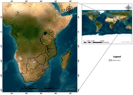
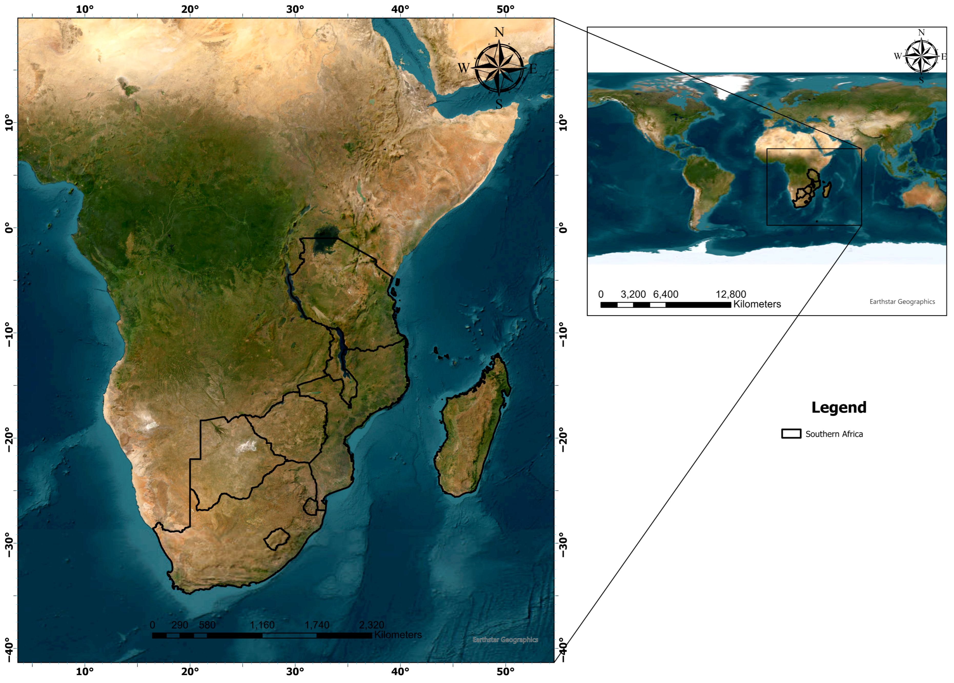
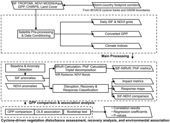
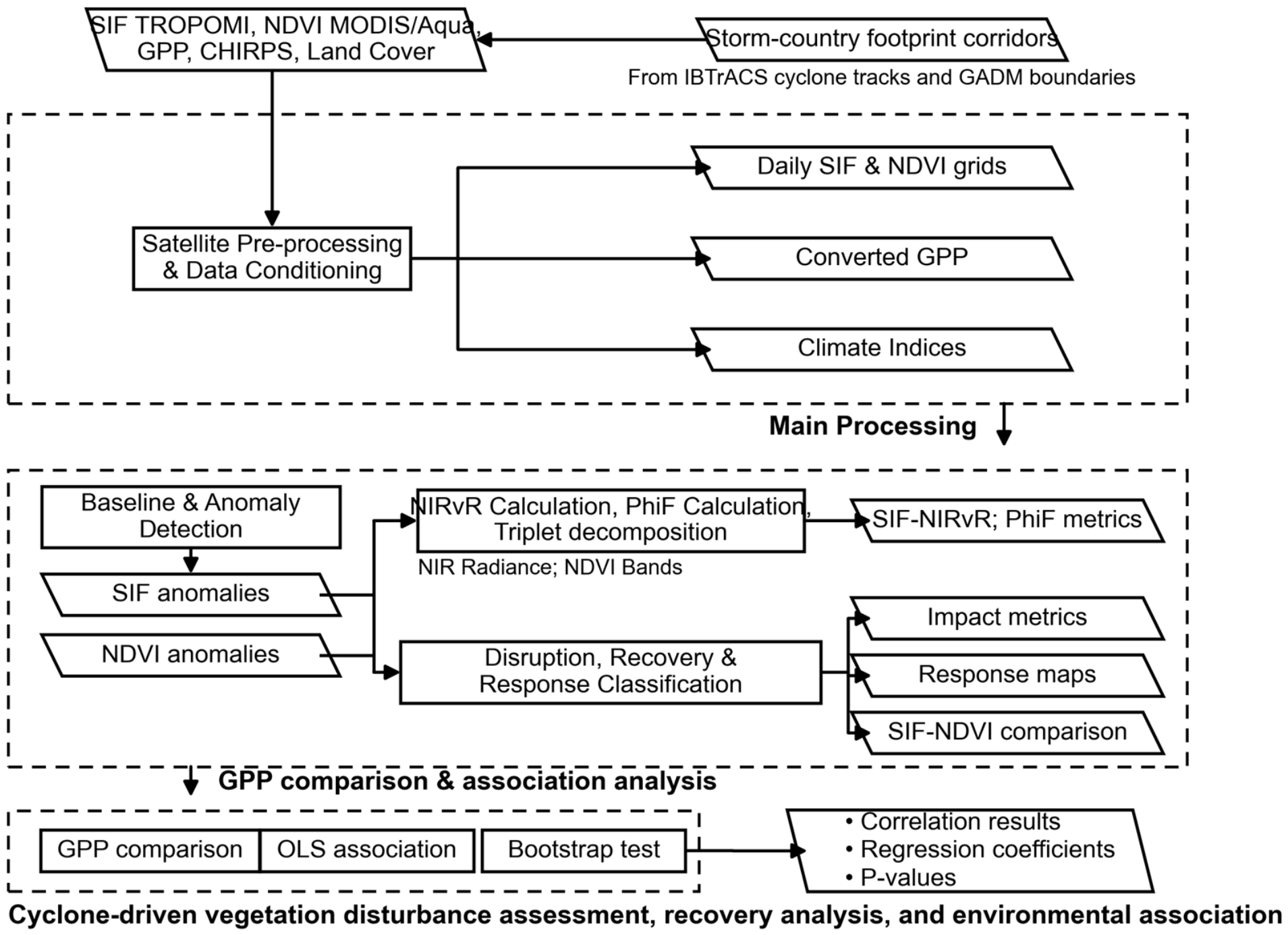
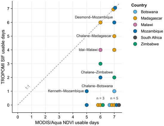
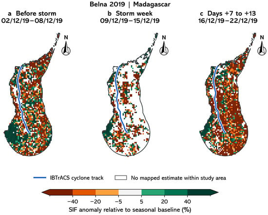
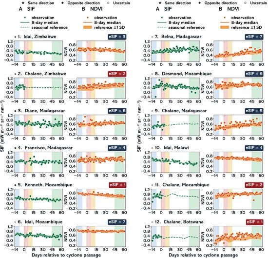
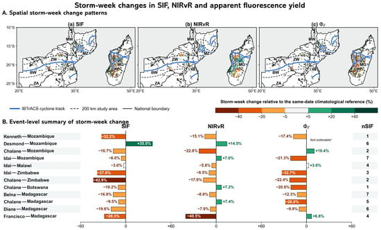
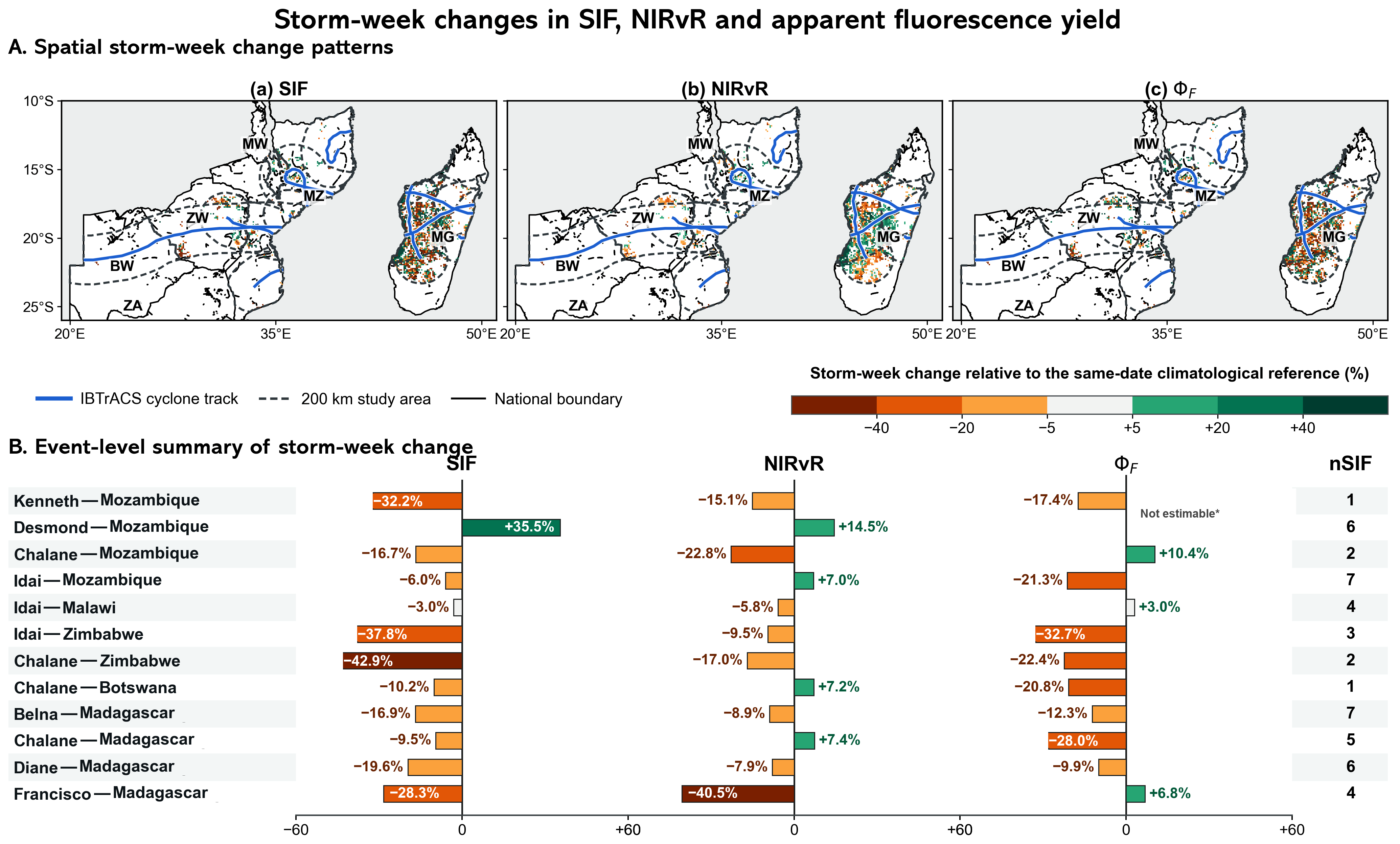

Disclaimer/Publisher’s Note: The statements, opinions and data contained in all publications are solely those of the individual author(s) and contributor(s) and not of MDPI and/or the editor(s). MDPI and/or the editor(s) disclaim responsibility for any injury to people or property resulting from any ideas, methods, instructions or products referred to in the content. |
© 2026 by the authors. Licensee MDPI, Basel, Switzerland. This article is an open access article distributed under the terms and conditions of the Creative Commons Attribution (CC BY) license.