A Single-Hydrophone Passive Localization Method in Sloping Shallow Water Using Warping-Transformed Eigenfrequency Analysis

Highlights

What are the main findings?

• A single-hydrophone method using warping-transformed eigenfrequencies from the energy density function enables simultaneous range and depth estimation of broadband impulsive sources in sloping shallow water.
• The extracted eigenfrequencies depend primarily on waveguide depth and average sound speed, showing inherent robustness against variations in other environmental parameters.

What are the implications of the main findings?

• The method significantly reduces the hardware and environmental knowledge required for source localization, making it practical for scenarios where deploying hydrophone arrays is infeasible.
• This approach offers a cost-effective and reliable solution for passive acoustic monitoring and remote sensing in complex shallow-water environments with varying seabed topography.

Abstract

Passive localization of broadband impulsive sources in shallow water is particularly challenging when using a single hydrophone, especially over a sloping seabed. This study presents a novel single-hydrophone localization method for broadband impulsive sources in sloping shallow water. The approach utilizes warping-transformed eigenfrequencies derived from the energy density function of received signals. A key innovation is the method’s capability for simultaneous range and depth estimation in sloping seabed environments, achieved through eigenfrequency pattern matching for range estimation and normalized amplitude matching for depth estimation. The method depends primarily on waveguide depth and average sound speed, enabling robust estimation while exhibiting inherent insensitivity to variations in other environmental parameters. Both simulated and experimental data from a winter sea trial in the East China Sea validate the performance of this dual-parameter estimation approach. The results demonstrate practical applicability for underwater acoustic monitoring and remote sensing in challenging shallow water environments with complex seabed topography.

1. Introduction

Due to the complexity of the underwater acoustic environment, shallow water passive localization has been a significant research focus in underwater acoustics. The current passive localization methods are mainly based on matched-field techniques [1,2], waveguide invariant [3], and normal modal dispersion properties [4,5]. The matched-field technique correlates the actual received acoustic field data with the copied acoustic field data calculated by the acoustic propagation model to achieve the position estimation of underwater targets [6]. This approach requires at least a hydrophone array to sample the spatial acoustic field and demands a large amount of computation and can lead to performance degradation or failure due to environmental parameter mismatch [7,8]. The method based on the waveguide invariant uses the stable interference fringes of the shallow waveguide acoustic field in the two-dimensional plane of distance and frequency to estimate the source distance, but it is insensitive to the source depth or needs a guide source with known distance [9,10]. The method based on array invariant exploits the multipath and dispersion effects in shallow waveguide, but has a large limitation on the ranging accuracy of long-range acoustic sources [11,12]. These methods, however, often rely on large-aperture arrays, known guide sources, or precise environmental matching, which limits their practical deployment in complex, range-dependent shallow-water environments.

The low-frequency broadband impulsive signal in the shallow waveguide is affected by the ocean medium and boundary conditions, producing superposition and dispersion of normal modes, and the dispersion characteristics contain information about the distance and depth of the sound source, as well as the environmental information of the waveguide [13]. However, such informative acoustic features are often weak and susceptible to environmental interference, making robust feature extraction and representation a significant challenge in underwater acoustic processing [14,15,16]. For broadband impulsive signals, warping-transform-based processing has been widely used to compensate for the nonlinear phase of individual normal modes, thereby enabling modal separation for source-range estimation and environmental-parameter inversion Bonnel et al. [5,17,18] first used it for distance estimation of impulse signals.

However, since the dispersion characteristics are affected by the extraction accuracy and are also sensitive enough to the environment parameters, the mismatch of the environment can also lead to inaccurate localization results. Wang et al. [19] use the invariance of the warping-transformed energy spectrum signal for distance estimation, but is limited to a flat seafloor and cannot estimate the depth. Guo et al. [20] use range-dispersion two-dimensional (2D) plane focus phenomenon of impulsive signals and the de-dispersion transform for distance estimation, but the method also requires accurate ocean environment parameters. Li et al. [21] use the time delay difference and group velocity slowness of different orders of normal modes to achieve the estimation of source distance, but the method assumes a constant seafloor phase shift parameter, which requires careful consideration in a practical environment.

In this paper, based on the broadband underwater acoustic impulsive signal propagating in shallow sea, a step-by-step estimation method of the distance and depth of the source is proposed by using the relationship between the modal dispersion characteristics of the normal mode and the location of the sound source. The warped energy density function of the received signal is only related to the depth and the average sound speed of the waveguide. Only when the assumed distance is equal to the actual one will the frequency characteristics after warping transformation be consistent with the theoretical value. Therefore, the distance estimation can be quickly implemented and extended to the case of a sloping seafloor. After obtaining the distance estimation, the energy relationship between the warped frequency peaks is then matched to obtain an estimate of the sound source depth. Looking forward, the robust source range and depth estimates provided by the proposed method could potentially serve as useful prior information for resource management in integrated underwater sensing and communication networks, where localization accuracy directly influences resource allocation strategies [22].

The remainder of this paper is organized as follows. Section 2 introduces the method for source distance and depth estimation using energy density functions. Section 3 performs simulation verification analysis in a typical shallow sea waveguide environment. Section 4 validates the analysis of the method using experimental data of East China Sea sound propagation in winter. Finally, discussion and conclusions are given in Section 5 and Section 6.

2. Theory and Methods

2.1. The Warping Transform of Energy Density Function

According to the normal mode theory [23], when a sound source emits a broadband pulse in the shallow water waveguide, the time domain of the received signal can be expressed as

$$y\left(t\right)={\displaystyle \sum _{m=1}^M}{A}_m\left(t\right){\mathrm{e}}^{j{\mathrm{\Phi }}_m\left(t\right)},$$

(1)

where ${\mathrm{\Phi }}_m$ is the time-evolving phase, $A_m$ is the instantaneous amplitude of mth mode. If the depth of the waveguide is d, the phase can be rewritten as

$${\mathrm{\Phi }}_m\left(t\right)=2\pi f_{cm}\sqrt{t^2-{(r/c)}^2},$$

(2)

where $f_{cm}$ is the cut-off frequency of mode m. The phase ${\mathrm{\Phi }}_m$ is a nonlinear function of time t. If the distance between the sound source and the receiver is also considered as a variable r, the received signal can be rewritten as

$$y(r,t)={\displaystyle \sum _{m=1}^M}{A}_m\left(t\right)e^{j2\pi f_{cm}\sqrt{t^2-{(r/c)}^2}}.$$

(3)

Previous studies have demonstrated that the received signal forms several nonlinear modes in the time-frequency domain, and that these modes are significantly related to the location of the sound source, which are called dispersion curves [5]. The warping transform is a widely used nonlinear transform to extract these curves and the operator in an ideal waveguide is [24]

$$h\left(t\right)=\sqrt{t^2+{(r/c)}^2},$$

(4)

However, bringing the warping operator of the ideal waveguide into the actual shallow waveguide will lead to theoretical errors, while the dispersion curves are also sensitive to the geoacoustic parameters, which will lead to less reliable positioning results.

In this case, using the energy density function for sound source localization is a better choice. The energy density function can be obtained by squaring the modulus of the received signal:

$$e_p\left(r,t\right)={\left|p\left(r,t\right)\right|}^2={\displaystyle \sum _{m=1}^M}{A}_m^2\left(t\right)+{\displaystyle \sum _{n=1}^M}{\displaystyle \sum _{m\ne n}^M}{A}_m\left(t\right)A_n\left(t\right)e^{j2\pi \left(f_{cm}-f_{cn}\right)\sqrt{t^2-{(r/c)}^2}},$$

(5)

The first term ${\sum }_{m=1}^M{A}_m^2\left(t\right)$ in the above equation represents the coherent part of the same-order normal mode. Since this term is concentrated around zero in the frequency domain, it can be safely ignored in subsequent calculations. The second term represents the coherent part of the different order normal modes, whose instantaneous phase $2\pi \left(f_{cm}-f_{cn}\right)\sqrt{t^2-{(r/c)}^2}$ is a time-varying term related to the cut-off frequencies of the mth and nth modes. To linearize this phase term and thereby reveal the constant EFs, the warping operator $h\left(t\right)=\sqrt{t^2+{(r/c)}^2}$ is used to process the energy density function to obtain

$$\left(W_h{e}_p\right)\left(r,t\right)={\left|{\displaystyle \frac{t}{h\left(t\right)}}\right|}^{{\displaystyle \frac{1}{2}}}\left[{\displaystyle \sum _{m=1}^M}{\displaystyle \sum _{n\ne m}^M}{A}_m\left(h\left(t\right)\right)A_n\left(h\left(t\right)\right)e^{j2\pi \left(f_{cm}-f_{cn}\right)t}\right].$$

(6)

In contrast to Equation (5), the time-evolving phase term in the above equation is compensated, causing the cross-mode coherence terms to manifest as a single frequency component $f_{m-n}=f_{cm}-f_{cn}$ in the frequency domain, which is also named as the eigenfrequency (EF). Because the cut-off frequency in shallow water is

$$f_{cm}={\displaystyle \frac{\left(2m-1\right)\overline{c}}{4d}},$$

(7)

where $\overline{c}$ is the mean sound speed in the waveguide and d is the depth of the waveguide, then the EF can be written as

$$f_{m-n}=f_{cm}-f_{cn}={\displaystyle \frac{(m-n)\overline{c}}{2d}}.$$

(8)

It can be seen that the EF is a function of the order difference of the different normal modes and is related to the sound speed as well as the water depth. It should be noted that after the Fourier transform of Equation (6), the EF represents the single frequency component formed by the combination of modes of the same order difference and the amplitude of the EF is superimposed by the amplitude of the considered modes, which is different from the warping transform of the received signal. Therefore, the smaller order difference between two modes, the smaller EF, the more corresponding mode combinations, and the larger the EF amplitude, and vice versa. Equation (8) shows that the EF are always $\overline{c}/2d$, $2\overline{c}/2d$, $3\overline{c}/2d$, etc. In general, the amplitude of $\overline{c}/2d$ is the largest because it is generated by the coherence of adjacent modes. For the other EFs, the amplitude strength relationship would be discussed in the following.

2.2. Distance Estimation Method for Sloping Seafloor

Although it can be seen from At first glance, Equation (8) suggests that the EF is a constant dependent solely on environmental parameters, seemingly unrelated to source localization. However, a solution emerges through the warping transform (Equation (4)). The warping transform needs to set the starting time t and the distance between source and receiver r, where t is the moment when the impulsive signal arrives. Equation (6) is obtained when r is accurate or known. When the assumed distance $r_s$ deviates from the true distance $r_0$, the energy density function becomes (ignoring the coherent part of the same order mode)

$$e_{\tilde{p}}(r_s,t)={\displaystyle \sum _{m=1}^M}{\displaystyle \sum _{n\ne m}^M}{\tilde{A}}_m\left(t\right){\tilde{A}}_n\left(t\right)exp\left[j2\pi \left(f_{cm}-f_{cn}\right)\times \sqrt{{\left(t+{\displaystyle \frac{r_0}{\overline{c}}}-{\displaystyle \frac{r_s}{\overline{c}}}\right)}^2-{\left({\displaystyle \frac{r_0}{\overline{c}}}\right)}^2}\right],$$

(9)

where ${\tilde{A}}_m\left(t\right)=A_m\left(t+r_0/\overline{c}-r_s/\overline{c}\right)$. Then the warped form with the assumed distance $r_s$ is

$$\begin{array}{cc}\hfill & \left(W_h{e}_{\tilde{p}}\right)(r_s,t)={\left|{\displaystyle \frac{t}{h\left(t\right)}}\right|}^{{\displaystyle \frac{1}{2}}}{\displaystyle \sum _{m=1}^M}{\displaystyle \sum _{n\ne m}^M}{\tilde{A}}_m\left(h\left(t\right)\right){\tilde{A}}_n\left(h\left(t\right)\right)\times \hfill \\ \hfill & exp\left[j2\pi \left(f_{cm}-f_{cn}\right)\sqrt{{\left(\sqrt{t^2+{\left({\displaystyle \frac{r_s}{\overline{c}}}\right)}^2}+{\displaystyle \frac{r_0}{\overline{c}}}-{\displaystyle \frac{r_s}{\overline{c}}}\right)}^2-{\left({\displaystyle \frac{r_0}{\overline{c}}}\right)}^2}\right].\hfill \end{array}$$

(10)

The Taylor expansion of warping operator $h\left(t\right)=\sqrt{t^2+{(r/c)}^2}$ yields

$$\tilde{h}\left(t\right)=\sqrt{t^2+{(r_0/c)}^2}=\sqrt{t^2+t_{r_0}^2}=t_{r_0}\sqrt{1+{\left(t/t_{r_0}\right)}^2}\approx t_{r_0}+t^2/2t_{r_0},$$

(11)

$$\left\{{\left(\sqrt{t^2+{\left({\displaystyle \frac{r_s}{\overline{c}}}\right)}^2}+{\displaystyle \frac{r_0}{\overline{c}}}-{\displaystyle \frac{r_s}{\overline{c}}}\right)}^2-{\left({\displaystyle \frac{r_0}{\overline{c}}}\right)}^2\right\}\approx {\left({\displaystyle \frac{t^2}{2r_s/\overline{c}}}\right)}^2+{\displaystyle \frac{r_0}{r_s}}{t}^2.$$

(12)

Considering that $t^2/(r_s/\overline{c})\ll 1$, substituting above equations into Equation (10) gives

$$\begin{array}{cc}\hfill & \left(W_h{e}_{\tilde{p}}\right)(r_s,t)={\left|{\displaystyle \frac{t}{h\left(t\right)}}\right|}^{{\displaystyle \frac{1}{2}}}{\displaystyle \sum _{m=1}^M}{\displaystyle \sum _{n\ne m}^M}{\tilde{A}}_m\left(h\left(t\right)\right){\tilde{A}}_n\left(h\left(t\right)\right)\times \hfill \\ \hfill & exp\left[j2\pi \left(f_{cm}-f_{cn}\right)\sqrt{{\displaystyle \frac{r_0}{r_s}}}\left(t+{\displaystyle \frac{t^3}{8r_s{r}_0/{\overline{c}}^2}}\right)\right].\hfill \end{array}$$

(13)

Compared Equation (6), the assumed EF can be defined as

$${\tilde{f}}_{m-n}\left(r_s\right)\approx \sqrt{{\displaystyle \frac{r_0}{r_s}}}{f}_{m-n}.$$

(14)

This equation establishes a direct functional relationship between the assumed distance $r_s$, the true source distance $r_0$ and the respective EFs, while the theoretical EF $f_{m-n}$ can be calculated from the known environment parameters by Equation (8). In practice, $r_0$ is unknown. By assuming a trial range $r_s$ in the warping operator, we compute a warped spectrum whose peak frequencies, termed assumed EFs ${\tilde{f}}_{m-n}\left(r_s\right)$, will coincide with the theoretical values fm-n only when $r_s=r_0$. This forms the basis of our range estimation. Then the distance estimation formula can be written as

$$r_0=r_s{\left({\displaystyle \frac{{\tilde{f}}_{m-n}\left(r_s\right)}{f_{m-n}}}\right)}^2.$$

(15)

In addition, considering that the conditions of a flat seabed in the actual environment are often difficult to meet, a sloping seabed waveguide with slow horizontal change is assumed, where the water depth changes from $d_1$ to $d_2$. For a linearly sloping seabed, Qi et al. [25] derived a precise expression for modal instantaneous frequency $f_m\left(t\right)$. Integration leads to the exact instantaneous phase ${\mathrm{\Phi }}_m\left(t\right)$,

$${\varphi }_m\left(t\right)=\pi {\displaystyle \frac{(2m-1)r}{2(d_2-d_1)}}\left(arcsin\left({\displaystyle \frac{{(d_2-d_1)}^2{t}^2/t_r^2-(d_1^2+d_2^2)}{2d_1{d}_2}}\right)+arcsin1\right).$$

(16)

When the propagation distance is large, the signal’s arrival time $t_r$ is much greater than its modal time spread $\tau$. This allows a small-argument approximation of the above arcsine function. Applying this long-range approximation leads directly to a simplified instantaneous phase ${\varphi }_m\left(t\right)\approx 2\pi {\displaystyle \frac{(2m-1)c}{4\sqrt{d_1{d}_2}}}\sqrt{t^2-t_r^2}$. Comparing this with the standard warping phase form in Equation (2), the modal cut-off frequency of mth in a sloping waveguide is immediately identified

$$f_m={\displaystyle \frac{(2m-1)\overline{c}}{4\sqrt{d_1{d}_2}}}.$$

(17)

Then, substituting Equation (17) into Equation (8), the EF of the energy density function under the condition of slow horizontal variation of depth can be obtained as

$$f_{m-n}=f_{cm}-f_{cn}={\displaystyle \frac{(m-n)\overline{c}}{2\sqrt{d_1{d}_2}}}.$$

(18)

The distance estimation steps for the sound source can be summarized as follows:

(1)

The mean sound speed in the waveguide is obtained from CTD measurements or historical data, and it is subsequently employed to compute the theoretical EF $f_{m-n}$ using Equation (8) or Equation (18).

(2)

Computing the energy density function of the received signal, then performing the warping transform and Fourier transform with different assumed distances $r_s$ to obtain the assumed EFs ${\tilde{f}}_{m-n}\left(r_s\right)$.

(3)

Using Equation (15) to estimate the distance $r_0$, and averaging the results to obtain the final estimation.

In practice, a set of assumed distances $r_{s,i}$ is pre-defined to mitigate random errors when applying Equation (15). In the simulation process, the assumed range $r_{s,i}$ is uniformly sampled within ±50% of the true range, with a step size of 1 km. This process yields a set of range estimates $r_{0,i}$ and the final distance estimate is subsequently obtained by averaging these results

$$r_0={\displaystyle \frac{1}{I}}{\displaystyle \sum _{i=1}^I}{\left({\displaystyle \frac{{\tilde{f}}_{m-n}\left(r_{s,i}\right)}{f_{m-n}}}\right)}^2{r}_{s,i}.$$

(19)

where I is the number of assumed distances.

2.3. Depth Estimation Method for Sloping Seafloor

Estimation of sound source depth in a shallow water environment usually requires hydrophone arrays with larger apertures to obtain a sufficient amount of spatial information about the underwater acoustic field. Using a single hydrophone to estimate the source depth is relatively more difficult but not impossible. The mode energy has been demonstrated to be related to the source and receiver depth [26,27].

At the same time, it can be found that the characteristic spectral peaks of the energy density function in Section 2.2 are still the coherent superposition between the corresponding mode group amplitudes. For this reason, the EF components can also be used to perform sound source depth estimation by matching the peak amplitude relationship of different orders of EFs.

Assume that the energy density function of the received signal has n EF peaks in the spectrum after the warping transform $a_{f_n}$, $n=1,2,\dots ,N$. After normalization using the maximum value, the EF peak ratio vector is

$$\mathbf{a}={\left[a_{f_1},a_{f_2},a_{f_3},\dots a_{f_n}\right]}^T.$$

(20)

In practice, due to the decrease in the signal-to-noise ratio, only the first few orders of EF peaks are usually observed in the spectrum, which will be discussed later.

Considering a set of hypothetical sound source depths $z_j$, $j=1,2,\dots ,J$, the received signal $y\left(t\right)$ can be computed by the sound field propagation model. Then using the approaches in Section 2.2, the predicted EF peak ratio can be obtained as

$$\mathbf{a}\left(z_j\right)={\left[a_{f_1}\left(z\right),a_{f_2}\left(z\right),a_{f_3}\left(z\right),\dots a_{f_n}\left(z\right)\right]}^T,$$

(21)

and the objective function for source depth estimation is

$$E\left(z_j\right)={\left|\mathbf{a}-\mathbf{a}\left(z_j\right)\right|}^2.$$

(22)

By matching this objective function over the possible depths of the sound source, the depth estimation of the sound source can be obtained.

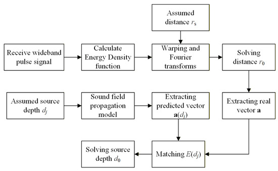
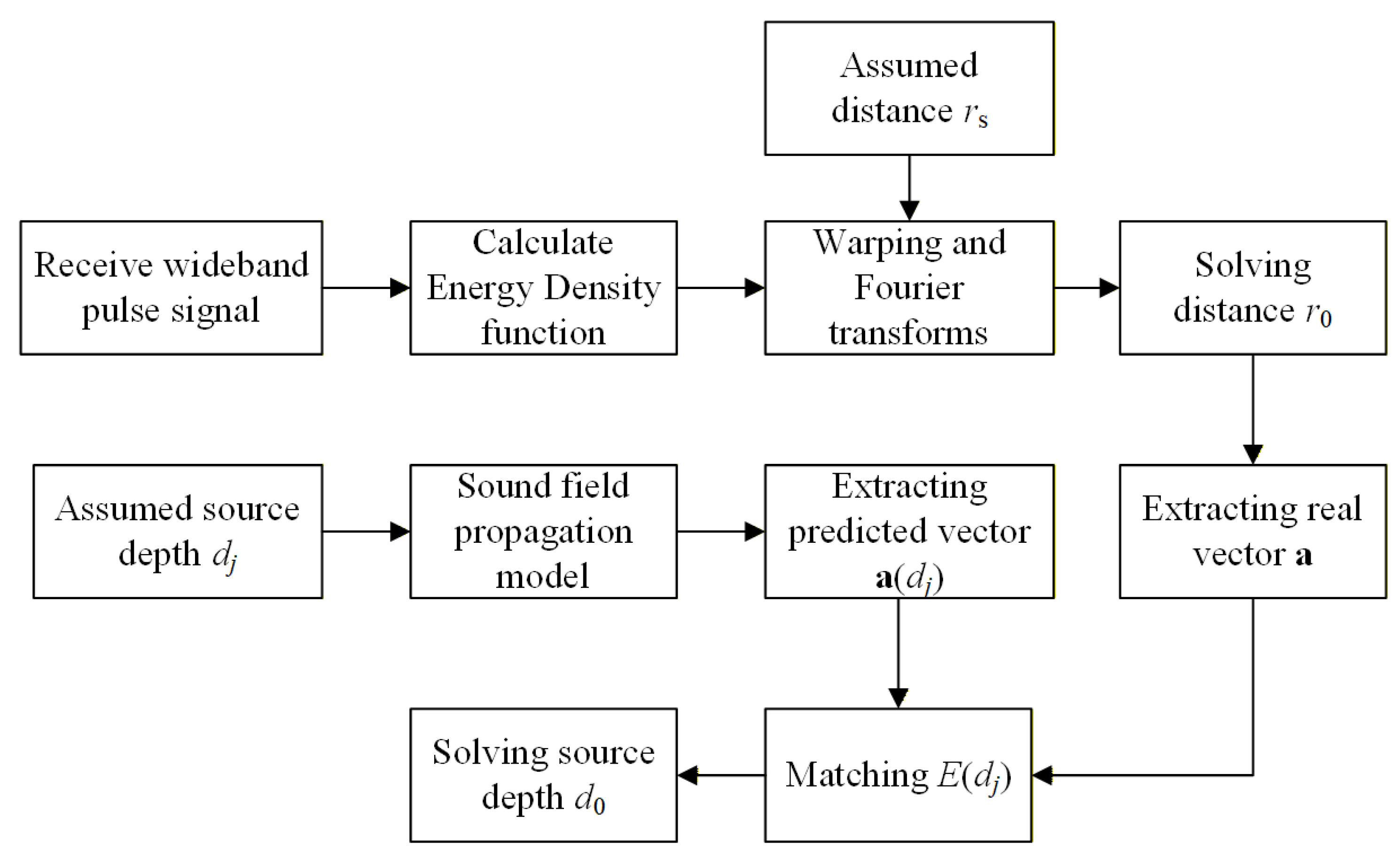
A flowchart of the sound source localization including distance and depth estimation is displayed in Figure 1.

Figure 1. Flowchart of the localization scheme.

3. Simulation Analysis

3.1. Range-Independent Waveguide

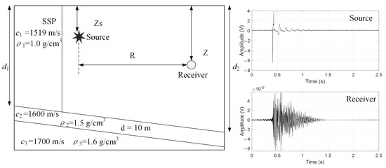
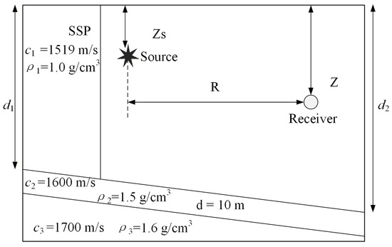
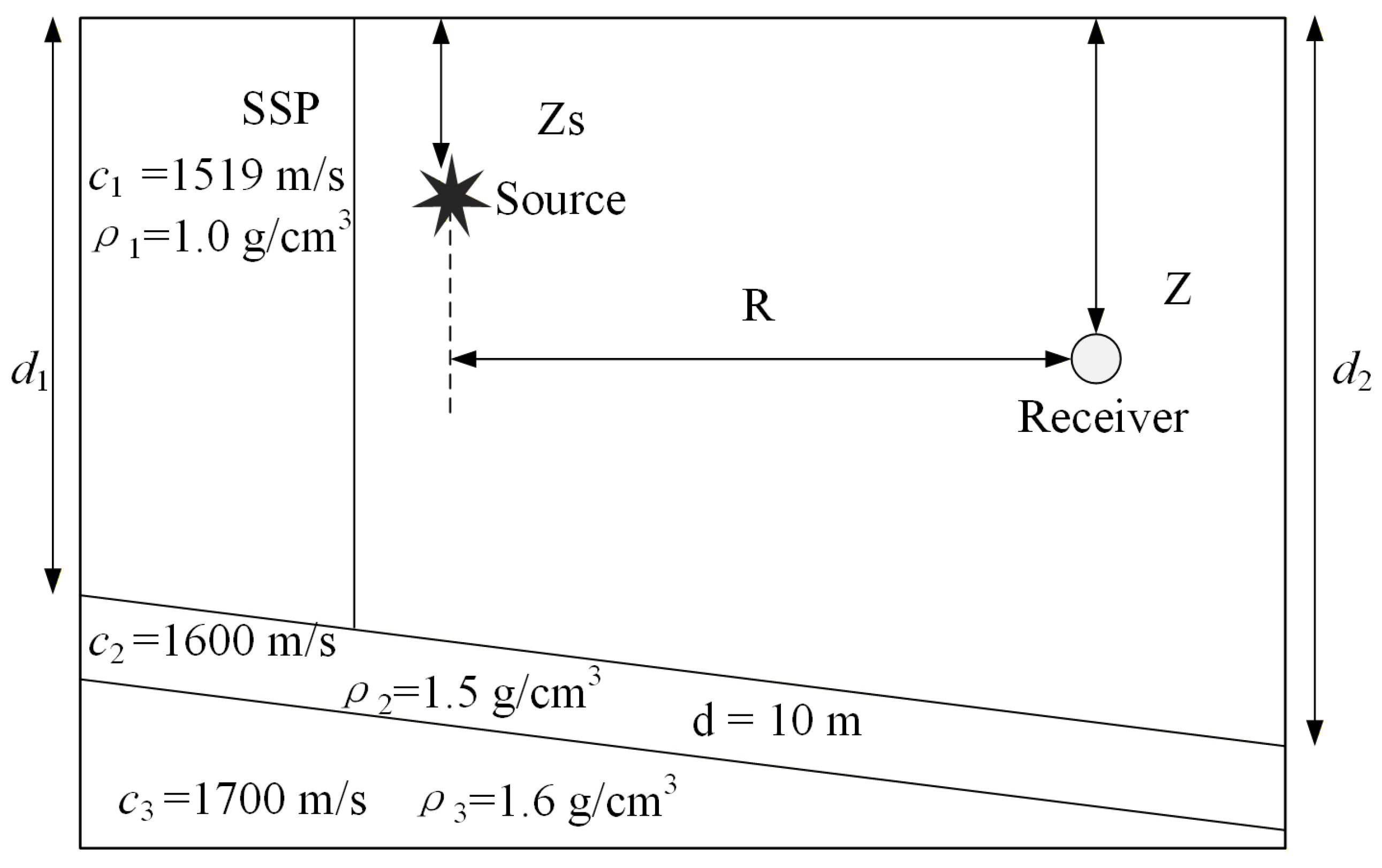
Consider a typical Pekeris range-independent waveguide environment as shown in Figure 2, which is relatively close to the real shallow water environment. The depth of the water column is 107 m and it has an invariable sound speed (1519 m/s). For the two-layer seabed, the sound speed, density and attenuation are 1600 m/s, 1.5 g/cm³ and 1700 m/s, 1.6 g/cm³ and 0.2 dB/$\lambda$. The simulated impulsive source was generated using a recording of a real air-gun system, characterized by an effective frequency band of approximately 20–200 Hz and a duration of less than 1 s. In the simulation environment, the sound source depth is 10 m and the distance from the receiving hydrophone is 25 km.

Figure 2. The range-independent simulation environment model and signal model; the right panel shows the time-domain waveforms of a typical airgun source signal and the received signal.

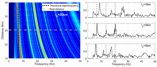
The received signal is synthesized by Kraken normal mode, shown in Figure 2. When performing the distance estimation, the distance of the sound source is unknown in advance, so the spectrum of the energy density function obtained by warping transform with different assumed distances is shown in Figure 3, where the receiving depth is 68 m.

Figure 3. The distance estimations in the simulation environment and the EF spectrum with different assumed distances after the warping transform. (left): normalized energy spectrum as a function of assumed range and frequency; the horizontal dashed line marks the true source range (25 km). (right): warped spectrum at the true range, with black dashed lines indicating the theoretical EF. The environment model is given in Figure 2.

In the frequency domain, several distinct bright stripes, representing the EFs, are observed. Their positions will move with a certain rule in the frequency domain with the difference of the assumed distance. Only when the assumed distance matches the set distance ($r_0$ = 25 km) in this simulation environment do the EF peaks align with the EF value calculated by Equation (8). Therefore, by extracting the EF values ${\tilde{f}}_{m-n}\left(r_s\right)$ at various assumed distance, the true source distance can be estimated using Equation (15).

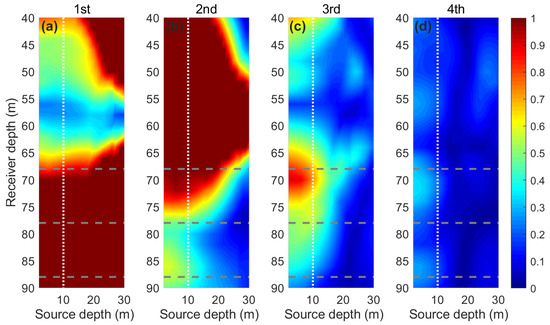
After obtaining the distance estimation, the next step is to estimate the depth of the sound source. To illustrate the principle of source depth estimation, first analyze the variation of the EF peaks on the sound source depth and the receiver depth plane. Figure 4 shows the variation in the normalized peaks of the first four EF peaks on that two-dimensional plane and the color scale has been shown as [0 1] in each subfigure.

Figure 4. The normalized peak amplitudes of the first four EF orders as functions of source depth and receiver depth in the simulation environment. (a) First-order EF; (b) second-order EF; (c) third-order EF; (d) fourth-order EF. In each subfigure, the white dotted line indicates the true source depth (10 m), and the three gray dotted lines mark the receiver depths of 68 m, 78 m, and 88 m. The source–receiver range is 25 km, and the color scale runs from 0 to 1.

As can be seen from Figure 4a, the first-order EF peak has good source depth resolution at relatively shallow receiver depths (above about 55 m); while at receiver depths below about 70 m, no matter what the sound source depth is, the amplitude of the first-order EF is consistently the strongest, resulting in its normalization to 1 and consequent loss of depth-discrimination ability. Therefore, when only the first-order EF peak is used for sound source depth estimation, there is a high probability that the sound source depth estimation fails.

A similar limitation arises when using only the second-order EF, as it only provides full depth discrimination for receivers deployed deeper than 70 m. Conversely, since the peaks of the third and fourth order EFs hardly ever become maximum terms in the spectrum, there is relatively complete source depth discrimination at all receiver depths. However, it must be pointed out that the peaks of the third and fourth EFs are usually weak after normalization, and the spectral peak error after the third order is larger in the real environment, it is not recommended to use only the higher-order peaks for sound source depth estimation. Based on the above reasons, the vector consisting of the peak ratio of the first four orders is used both in the simulation and subsequent experimental data processing for the estimation of sound source depth.

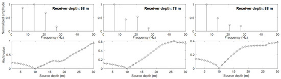
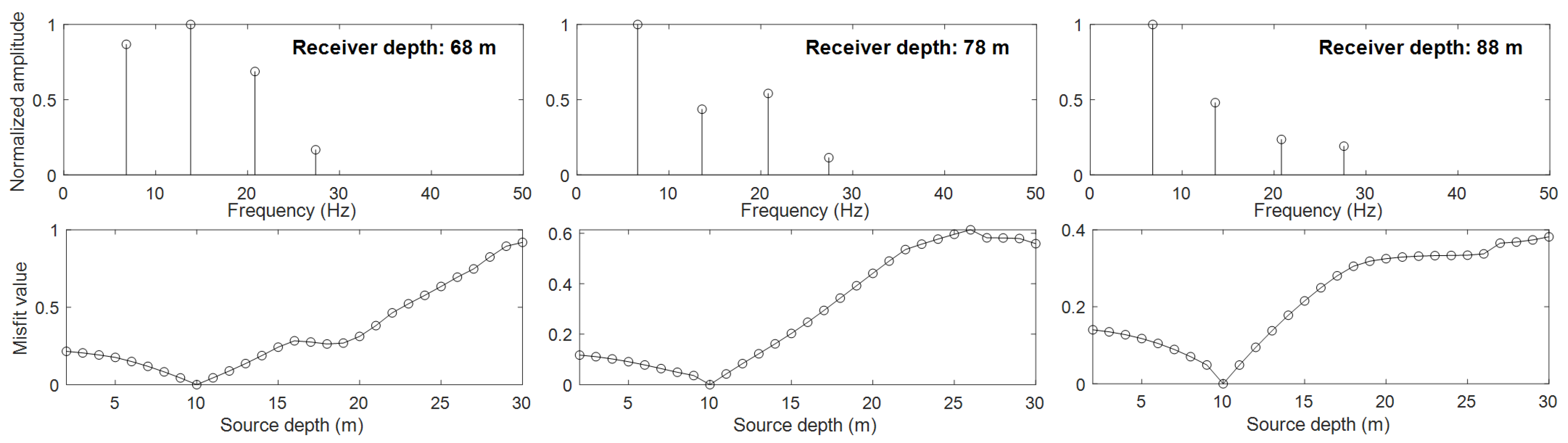
Then the simulation experiment of sound source depth estimation is carried out using a single hydrophone, where the sound source depth is 10 m. The hydrophones with different depths are used for comparison, and their positions are marked in Figure 4. The results of depth estimation are shown in Figure 5, where the estimated depth of the sound source is all 10 m at different receiver depths, showing good depth estimation accuracy. The receiver depths, from left to right, are 68 m, 78 m, and 88 m, corresponding to the horizontal dashed lines in each subfigure of Figure 4.

Figure 5. The results of estimation of sound source depth (10 m) by using different receiver depths (68 m, 78 m, 88 m) at the distance of 25 km in a simulation environment.

3.2. Range-Dependent Waveguide

To evaluate the applicability of the proposed method in a more realistic coastal environment, a slowly sloping seabed is considered, as shown in Figure 6. The water column sound speed profile and the seabed geoacoustic parameters in this waveguide model are identical to those used in Section 3.1. The only modification is the introduction of a sloping seabed by varying the water depths $d_1$ and $d_2$. Because the Kraken normal mode model is inherently limited in handling acoustic propagation in range-dependent environments, the RAM parabolic equation model is adopted to synthesize the received signals with the same recorded air-gun pulse under these conditions.

Figure 6. A typical sloping seabed environment, where $d_1$ and $d_2$ represent different depths along the slope.

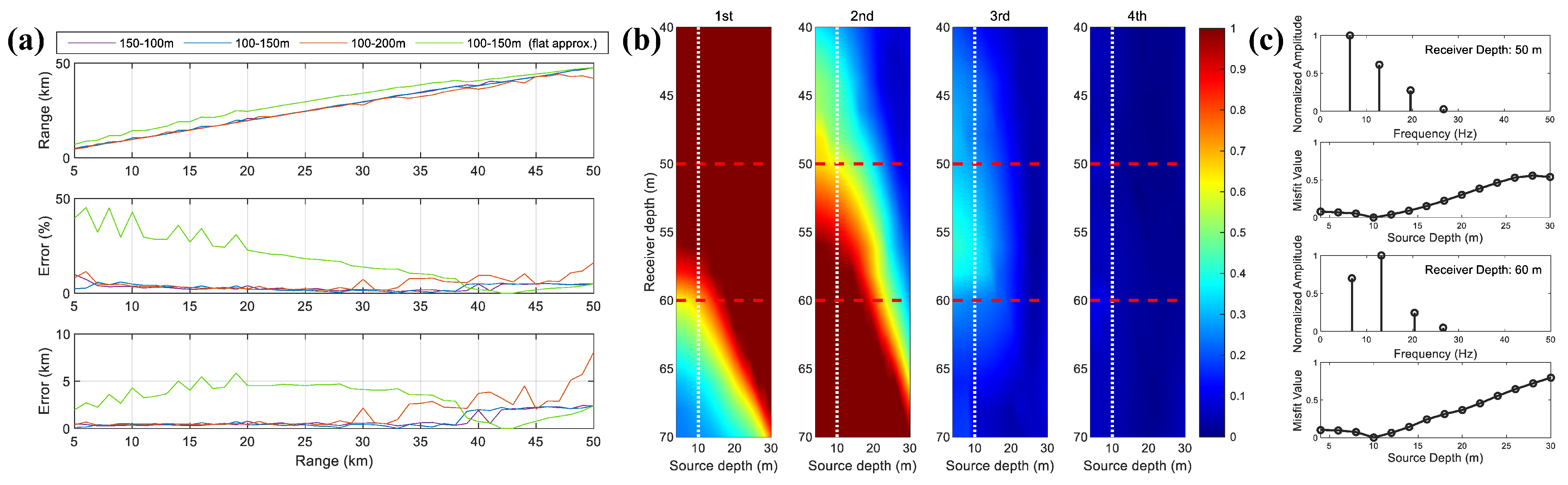
First, the capability of the proposed method for both distance and depth estimation under sloping-bottom conditions is validated, and the influence of different seabed slopes on distance estimation accuracy is compared. Three sets of slope parameters are considered: (1) $d_1=100$ m, $d_2=150$ m; (2) $d_1=100$ m, $d_2=200$ m and (3) $d_1=150$ m, $d_2=100$ m, where the total span of the simulated ranges R is 50 km. The comparison between the first and third sets corresponds to interchanging the source and receiver positions. For each of these three range-dependent waveguide models, the RAM parabolic equation model is used to synthesize the received signals at various ranges, and the range estimation is performed using the method described in Section 2.2.

Additionally, to compare the effects of Equations (8) and (18) on ranging accuracy, the received signals from the first environmental scenario are also processed with Equation (8) (which assumes a flat seabed) to calculate the eigenfrequency of the energy density function and subsequently estimate the distance. The resulting comparisons are shown in Figure 7.

Figure 7. The localization results in slope environments. (a) Comparison of distance estimation errors under different slope parameters and the flat-bottom assumption. From top to bottom: estimated range, relative error, and absolute error. (b) In the 100–150 m sloping-bottom environment, the first four orders of normalized EF peaks of the received signal at 30 km as functions of source and receiver depth. The white dashed line indicates the source depth, and the red dashed lines indicate the two receiver depths displayed on the right. (c) The results of estimation of sound source depth by using different receiver depths (50 m and 60 m).

It can be observed that Equation (18) is able to effectively estimate the depth-dependent eigenfrequency in all three sloping-bottom scenarios, yielding distance estimates with small errors, particularly at short ranges. The corresponding depth estimates are also accurate, further validating the method’s dual-parameter estimation capability. In contrast, Equation (8), which is based on the flat-bottom assumption, proves inadequate for handling such range-dependent bathymetry.

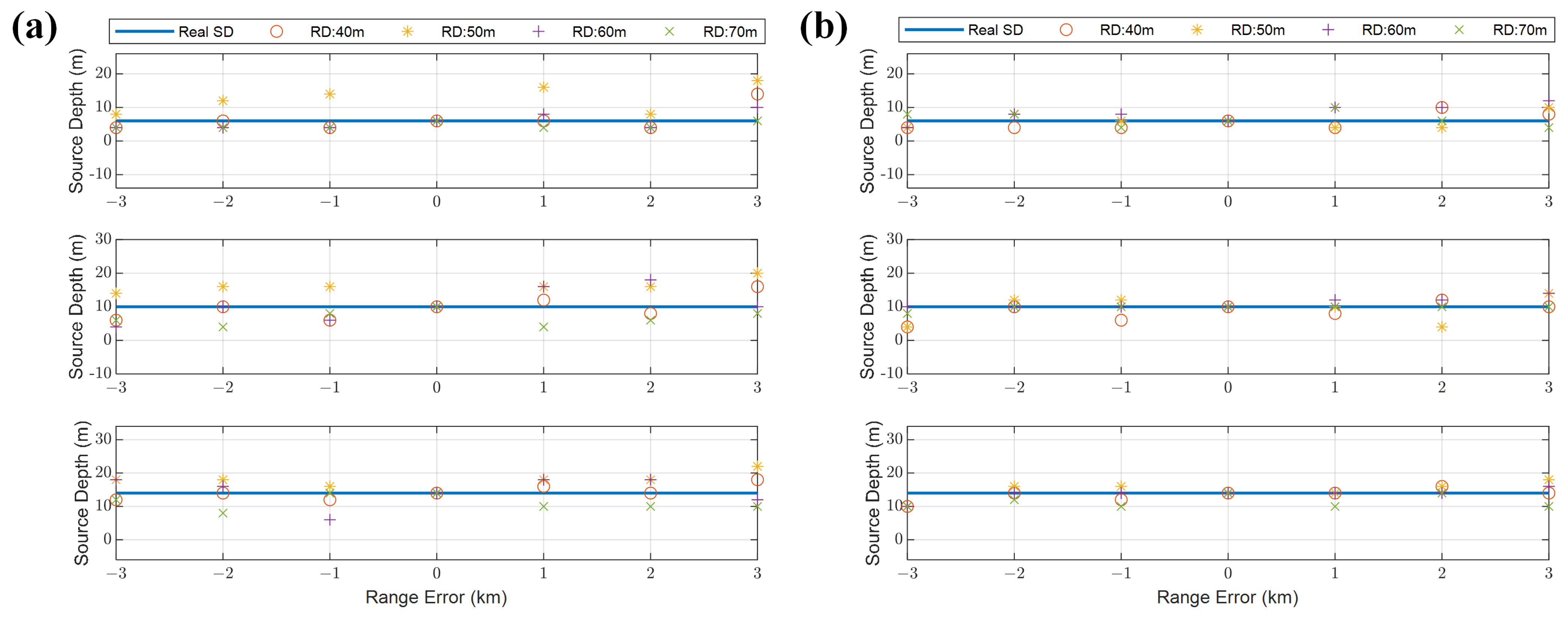
Following this, the influence of different parameters on depth estimation accuracy is examined. The first factor investigated is the sensitivity to considered is the distance estimation error. The localization procedure of the proposed method consists of two main steps: range estimation is performed first, followed by depth estimation. Since accurate distance information is required for depth estimation—specifically, to apply the warping transform to the energy density function and extract the EF peaks—two receiving ranges, 15 km and 30 km, are selected based on the first sloping-bottom scenario, and the source depth estimation results are analyzed as the distance estimation error varies from −3 km to +3 km. The results are shown in Figure 8. As shown in the figure, the distance estimation bias exerts a considerable influence on the depth estimation, and as the range increases (from 15 km to 30 km), the depth estimation error caused by the same distance estimation bias decreases significantly. When the range estimation bias is less than 10%, the depth estimation error can typically be kept within 10 m.

Figure 8. Deviation between the estimated source depths and the set values when range estimation errors are present in the received signals at 15 km (a) and 30 km (b) with the first sloping-bottom scenario. From top to bottom, the source depths are 5 m, 10 m, and 15 m, respectively.

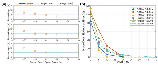
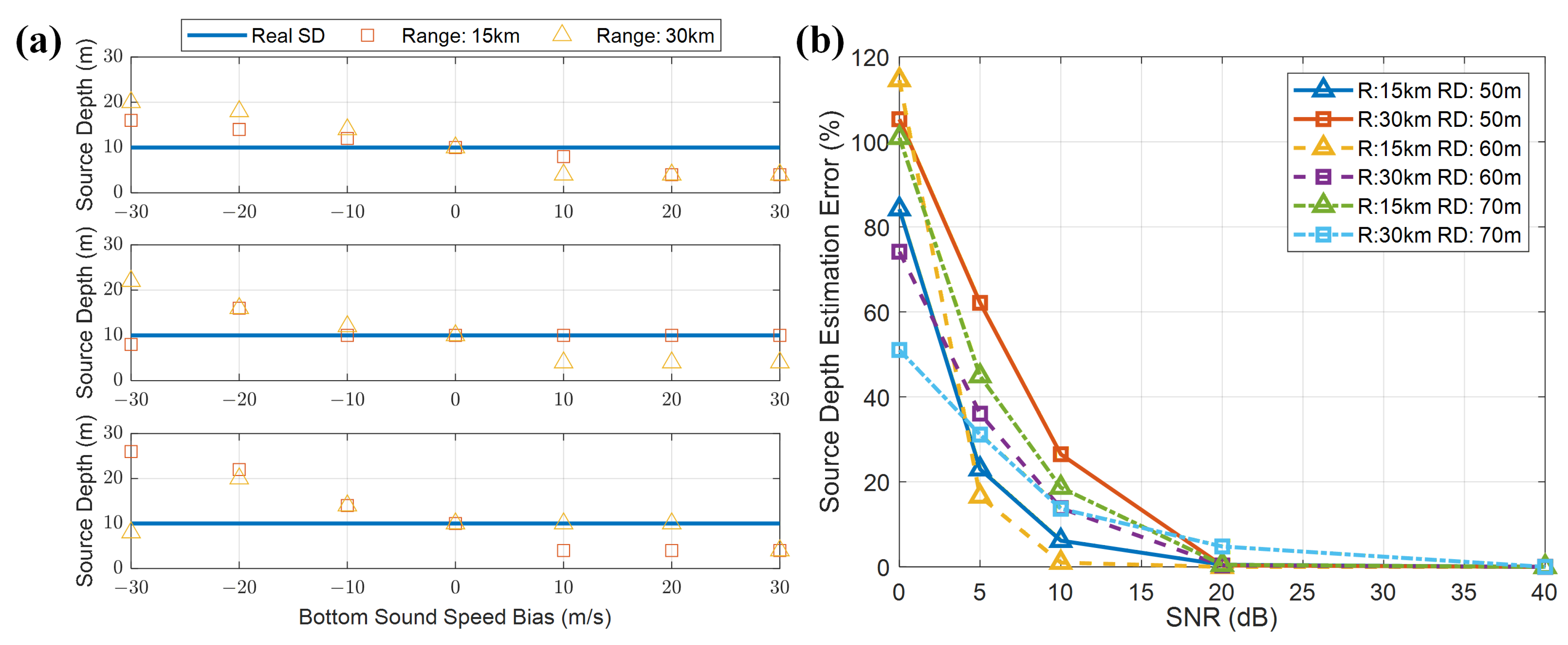
Next, the localization errors caused by the deviations of seafloor sediment parameters and the signal-to-noise ratio (SNR) of the received signal are analyzed. First, the effect of a ±30 m/s bias in the seafloor sound speed is examined. Since the formula used for range estimation has been shown to be insensitive to bottom parameters, the analysis focuses on the depth estimation error induced by the bottom deviation. A Monte Carlo simulation method is then employed to generate a large number of simulated signals with SNRs of 0 dB, 5 dB, 10 dB, 20 dB and 40 dB, and the relative error of the depth estimate as a function of SNR is analyzed. The waveguide model of the first sloping-bottom scenario is still adopted here, with receiving depths of 50 m, 60 m and 70 m. The results are shown in Figure 9.

Figure 9. Analysis of the influence of seafloor sound speed and received signal SNR on depth estimation. (a) Sound speed bias of ±30 m/s, with source-receiver ranges of 15 km and 30 km; from top to bottom, the estimated source depths for receiving depths of 50 m, 60 m, and 70 m are shown. (b) Relative error of the estimated source depth as a function of SNR from 0 to 40 dB.

As shown in Figure 9, a bias in the seafloor sound speed significantly affects the accuracy of source depth estimates. Specifically, an overestimated sound speed leads to an overestimated source depth, and vice versa. Meanwhile, when the SNR exceeds 10 dB, the relative error of the depth estimation can be substantially reduced to within 20%. It is worth noting that, in the comparative analysis of the two cases, the receiving depth also exhibits a rather complex influence mechanism, which may be related to the fact that the normal modes are excited with different strengths at different depths, and this topic deserves further investigation.

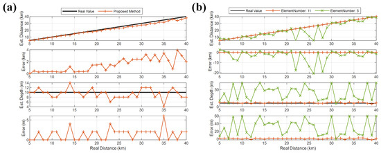
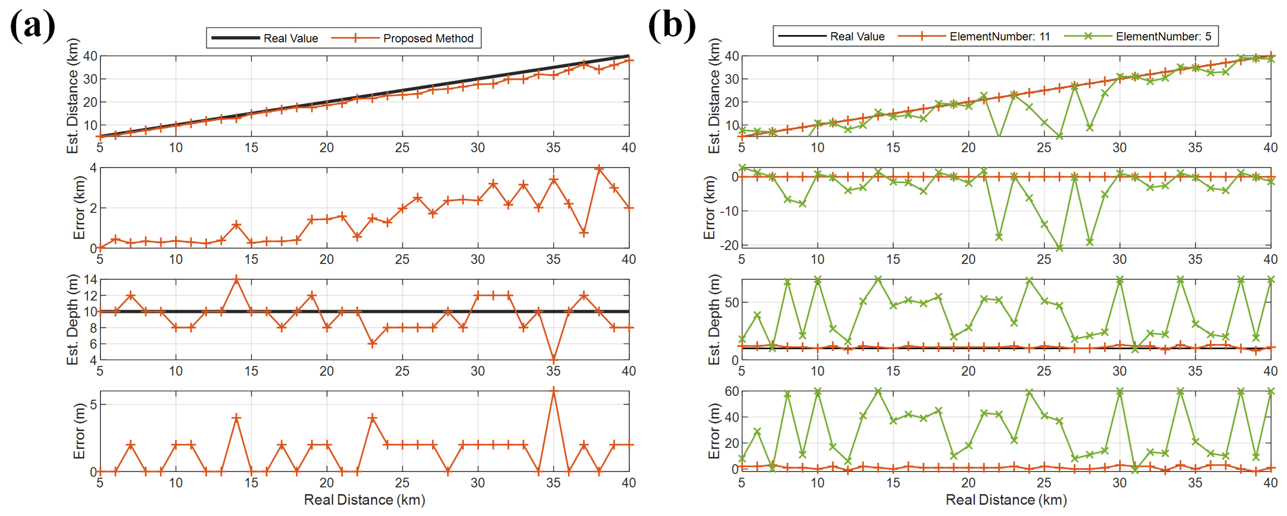
Finally, the proposed method is compared with the classical matched-field processing (MFP) localization method, again using the first sloping-bottom scenario for the simulation analysis, shown in Figure 10. First, the received signals at various ranges are generated from an airgun source deployed at a depth of 10 m. To approximate a realistic noisy environment, the SNR is set to 10 dB. Then, source localization is performed on the data from one of the hydrophones following the steps described in Section 2.2 and Section 2.3 and the result is shown in Figure 10a, while the localization result obtained by the matched-field method is shown in Figure 10b. For the MFP method, 11 frequency points in the band spanning 20–200 Hz were processed. Two configurations of a virtual vertical line array, with 5 and 11 elements, were considered. Comparing the results, it can be seen that with only a single hydrophone, the proposed method achieves better localization accuracy than the 5-element line array, and its range estimation accuracy is close to that of the 11-element line array while its depth estimation accuracy is significantly better, indicating that the proposed method offers certain advantages in sloping-seafloor scenarios.

Figure 10. Comparison of the localization performance between the proposed method and the matched-field method for a received signal with an SNR of 10 dB in the same sloping-seafloor waveguide, with the source depth fixed at 10 m. (a) Localization result and error of the proposed method. (b) Localization results and errors of the matched-field method for array configurations with 11 and 5 elements, respectively, where the distance estimation error of the matched-field method is 0 when using an 11-element array.

4. Verification of Experiment Data

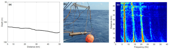
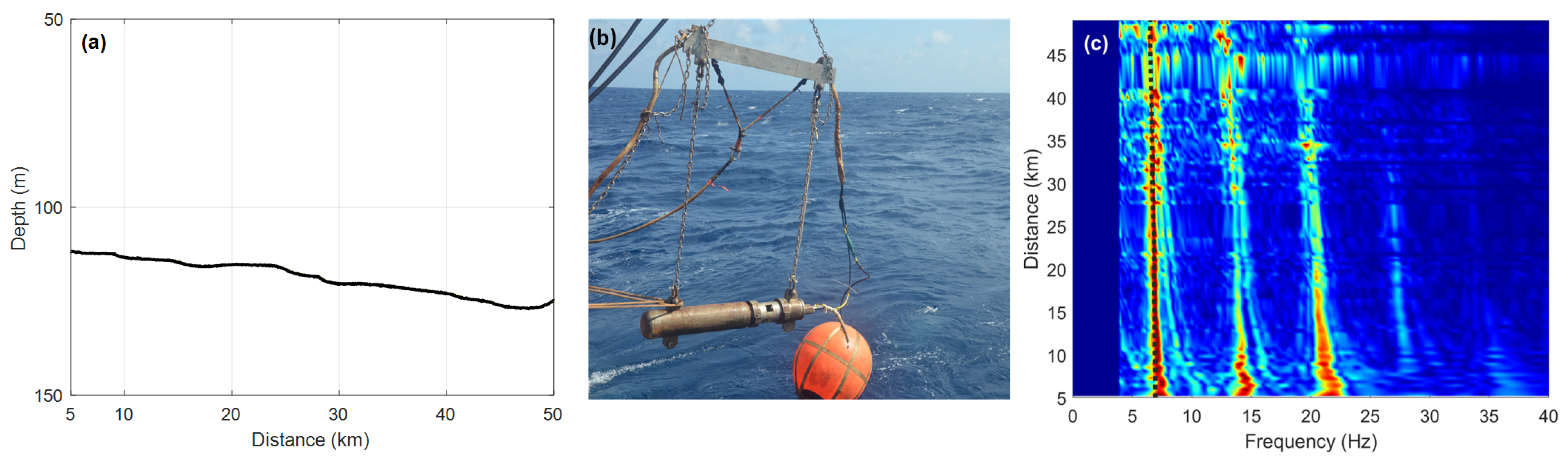
A shallow sea acoustic propagation experiment was conducted in the East China Sea in January 2015 and the data were used to validate the proposed localization method. During the experiment, the research vessel towed an air-gun sound source emitting broadband impulsive signals at fixed intervals and gradually moving away from the receiving hydrophones along a straight survey line. The research vessel sailed at a constant speed, and the ship-mounted depth sounder continuously recorded the bathymetry along the track. The air-gun source recorded its GPS position at each shot, while the GPS position and water depth of the receiving hydrophones were precisely logged during the deployment of the subsurface buoy array. The source–receiver distance for each shot was calculated by combining the GPS records from both the source and receiver. The bathymetry profile along the track (Figure 11a) was constructed from the depth-sounder data. About seven CTD stations were occupied along the survey line. The sound-speed profiles measured at these stations were depth-averaged to obtain the mean sound speed $\overline{c}=1519$ m/s; the inter-station variability of the depth-averaged sound speed was within ±2 m/s, indicating a well-mixed water column consistent with winter conditions in the East China Sea. This small variability supports the use of a single representative average sound speed for the entire track. The subsurface buoy array included hydrophones at multiple depths, each equipped with a temperature–depth (TD) sensor providing accurate real-time depth readings. The environmental parameters of the waveguide are essentially the same as those in Section 3.

Figure 11. The experimental environment and EF spectrum along the survey line. (a) Bathymetry profile along the track, showing a gradual deepening slope from 5 km to 50 km. (b) Air-gun sound source system used in the experiment. (c) Normalized EF spectrum of the energy density function after warping transform for received signals at ranges of 10–50 km (receiver depth: 66 m); the color scale represents normalized amplitude, and the black dotted line marks the theoretical first-order EF.

Because the trajectory of the survey line is a gradual deepening slope from 5 km to 50 km, as shown in Figure 11a, the theoretical EF of the energy density should be computed by Equation (18). Figure 11b shows the air-gun sound source system used in the experiment and Figure 11c shows the EF spectrum of the energy density function after warping transform for all received signals within 10–50 km (receiver depth 66 m). The slow change in sea depth over distance causes the EF to change, and the theoretical EF calculated using Equation (18) (black dotted line in Figure 11c) is more consistent with the real situation.

Since the precise GPS position was recorded at each shot, the exact interval does not affect the range determination. The received acoustic data were continuously recorded. Individual shot signals were segmented from the continuous recording based on signal energy: for each expected shot arrival window, the segment boundaries were chosen to encompass both the signal onset and the trailing modal dispersion tail. Each segmented window was verified by inspecting its time-frequency spectrogram to confirm that the full modal arrival structure was captured.

For each shot, the water depth at the source position $d_1$ and at the receiver position $d_2$ were obtained by interpolating the bathymetry profile (Figure 11a) at the corresponding GPS coordinates. The geometric-mean depth $\sqrt{d_1{d}_2}$ was then used in Equation (18) to compute the theoretical EF for that specific source–receiver geometry. The warping transform requires a starting time $t=0$ aligned with the signal’s arrival. In this study, this starting time was determined automatically by analyzing the normalized cumulative energy of the received signal. The instant at which this energy reached 60% of its maximum value was selected as the warping origin. This threshold was chosen empirically to balance the inclusion of the early-arriving modal energy against the exclusion of pre-signal noise. The window length was set to cover the full modal arrival spread, extending from the selected starting time through the trailing portion of the dominant modal energy, as verified by time-frequency analysis. This procedure ensures that the warping operator is correctly synchronized with the physical arrival of the acoustic pulse.

The EF peaks in the warped spectrum were identified through an automated procedure with visual verification. First, the theoretical frequencies of the first four EFs were computed via Equation (18) for the given source–receiver geometry. A frequency search window was then defined around each theoretical EF value. The local spectral maximum within each window was identified as the corresponding EF peak, provided its amplitude exceeded a pre-defined threshold relative to the local noise floor. All detected peaks were subsequently verified by visual inspection of the warped spectra.

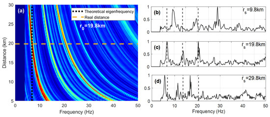
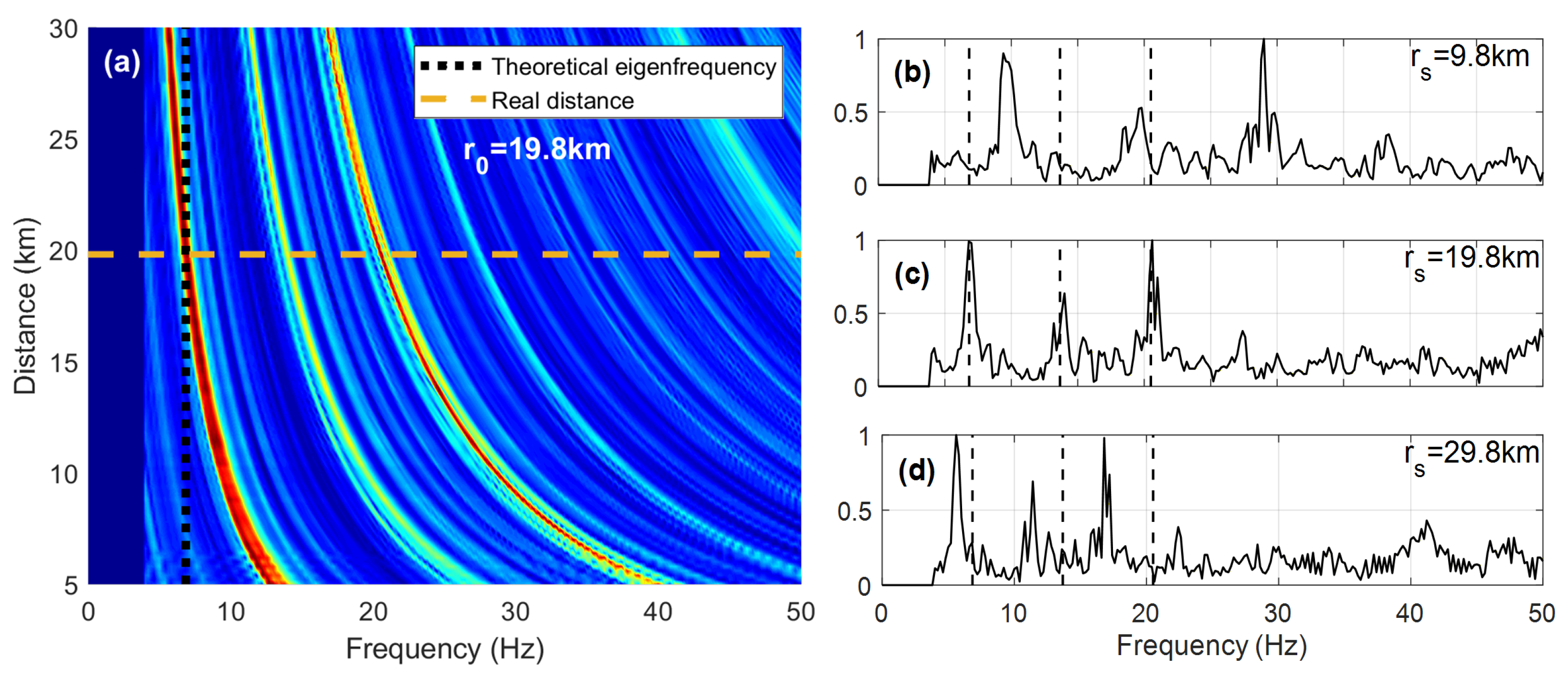
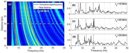
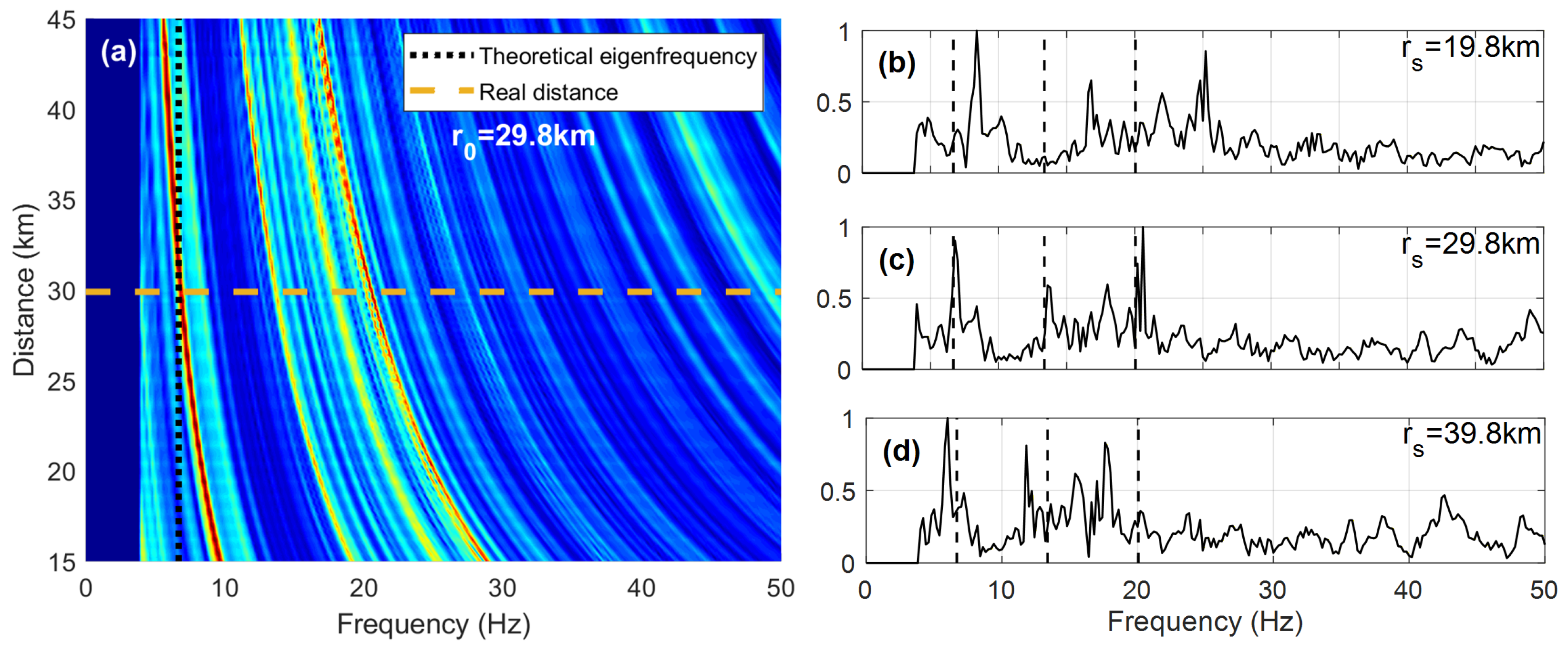
To illustrate the ranging capability, Figure 12 and Figure 13 give the EF spectrum of received signals at distances of 19.8 and 29.8 km with different assumed distances after warping transformation. As the air-gun source energy is mainly within 20–200 Hz and the high-energy modes are concentrated in this band, the signal is passed through a bandpass filter with 20–200 Hz to remove low-frequency interference and higher-order modal terms. As seen in Figure 12a, the EF of each order gradually recovers to the theoretical values as the assumed distances approach the true values from the small or large places, and so does Figure 13a. The theoretical EF of $f_1$ is 6.83 Hz at a source distance of 19.8 km and 6.68 Hz at 29.8 km, which is in good agreement with the first peak position corresponding to the real distance spectrum. Due to the band-pass filtering, the peaks of EFs after the third order decrease significantly, and the background noise in the long-range transmission environment causes the EF peaks after the third have somewhat offset from the theoretical value, so only the first peak needs to be selected as a reference when estimating the distance.

Figure 12. The spectrum obtained by warping transform of the energy density function for the signal at a distance of 19.8 km (receiver depth: 66 m). (a) Normalized EF spectrum as a function of assumed range and frequency; the color scale represents normalized amplitude; the horizontal dashed line marks the true range and the vertical dotted line marks the theoretical first EF. (b–d) Warped spectra at assumed ranges of 9.8 km, 19.8 km, and 29.8 km, respectively; black dashed lines indicate the theoretical values of the first three EFs.

Figure 13. The spectrum obtained by warping transform of the energy density function for the signal at a distance of 29.8 km (receiver depth: 66 m). (a) Normalized EF spectrum as a function of assumed range and frequency; the color scale represents normalized amplitude; the horizontal dashed line marks the true range and the vertical dotted line marks the theoretical first EF. (b–d) Warped spectra at assumed ranges of (b) 19.8 km, (c) 29.8 km, and (d) 39.8 km; black dashed lines indicate the theoretical values of the first three EFs.

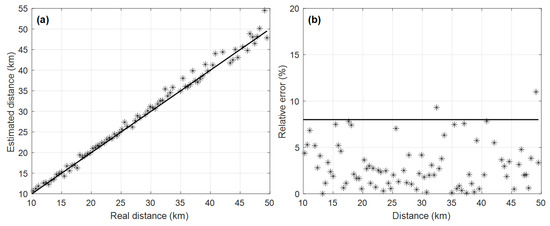
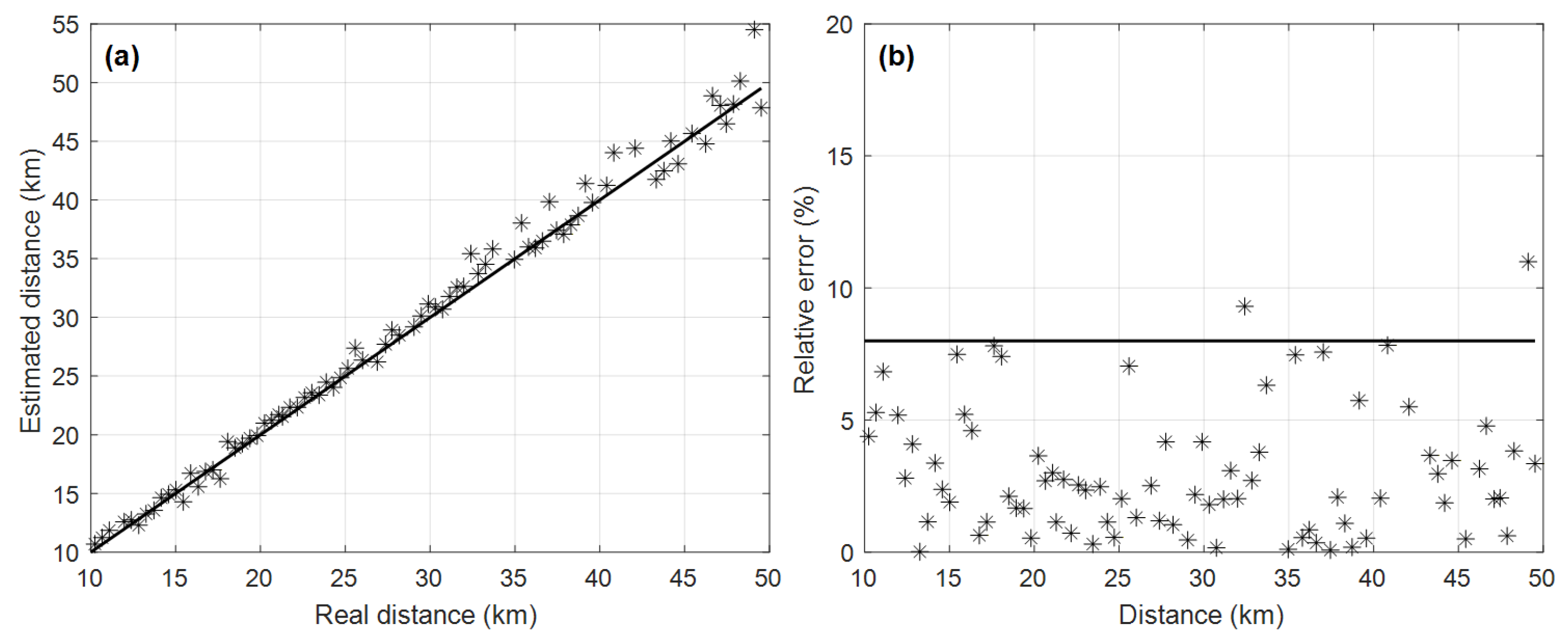
For range estimation, the first EF peak was used as the reference. After obtaining the spectrum corresponding to several assumed distances in succession, the first EF is extracted using the automated peak-detection procedure described above and the distance estimate is calculated using Equation (19), and finally the multiple valuations are averaged as the final result for this signal. This is repeated until all signals are processed, and the distance estimation results are obtained as shown in Figure 14. The results show that the distance accuracy of most of the signals is satisfactory, except for individual signals.

Figure 14. Sound source distance estimation results on the survey line. (a) Estimated source distance versus GPS-measured distance; the dashed diagonal line indicates the ideal $y=x$ relationship, and asterisks represent individual shot estimates; (b) Relative error of distance estimates for each shot, expressed as percentages.

Based on the obtained distance estimation results, source depth estimation was performed following the flowchart in Figure 1. By traversing the depth of the air-gun source signal and matching the peak ratio vector of the EF using Equation (22), the depth estimation of the air-gun source at different distances can be obtained.

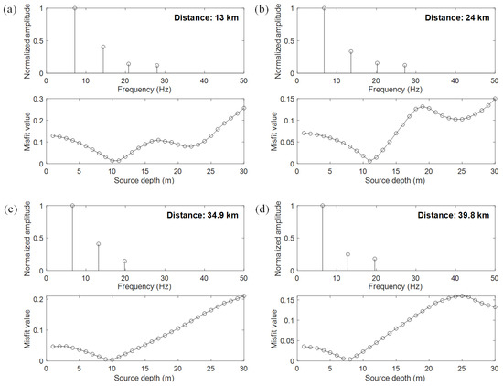
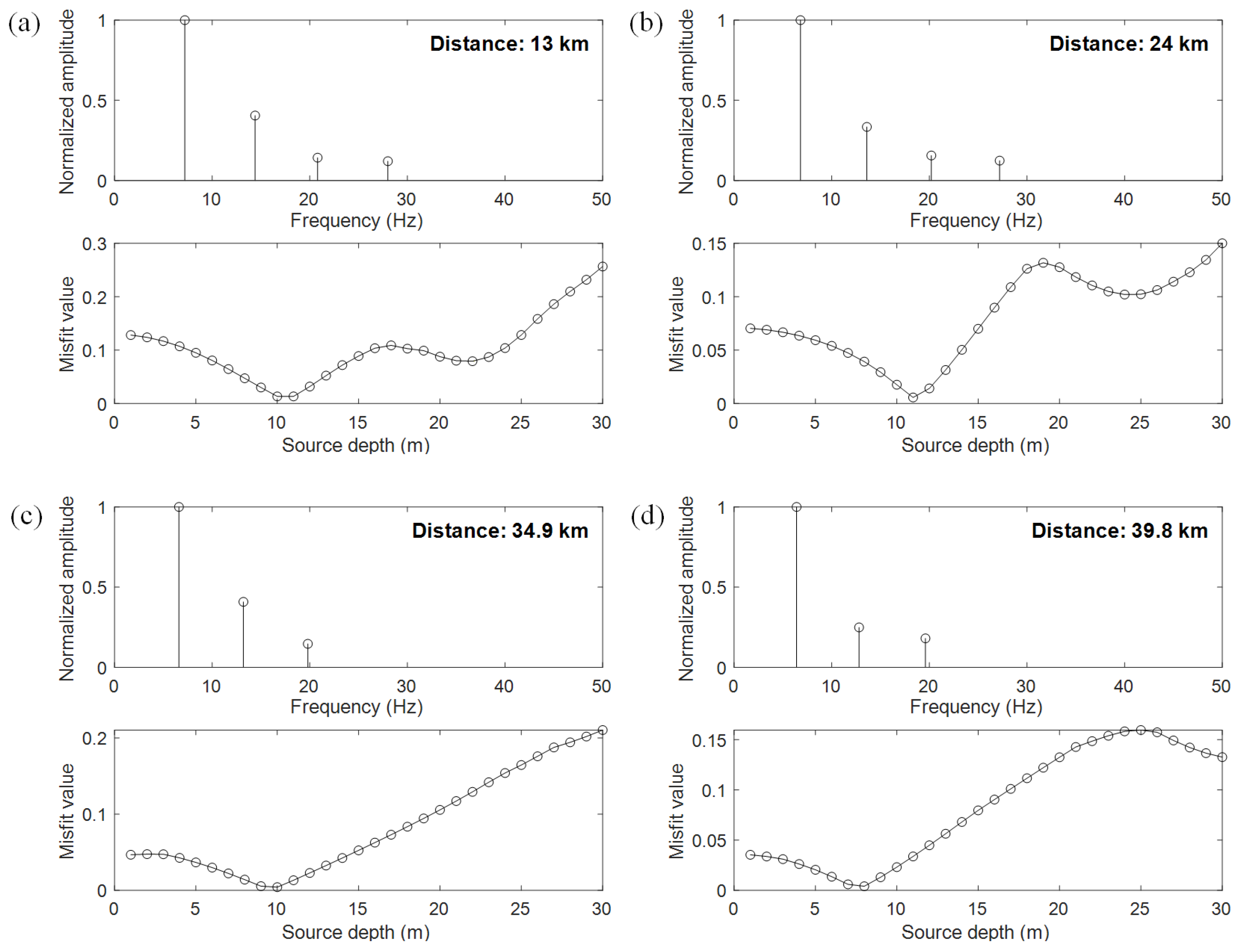
The EF peak ratio from the warped energy density function and the corresponding source depth matching results at various distances are shown in Figure 15, where the receiver depth is 96 m. It can be seen that the depth of the air-gun source is most likely to be around 10 m, which is consistent with the source depth setting recorded in the experimental log.

Figure 15. Sound source depth estimation results for air-gun signals at different distances: (a) 13 km; (b) 24 km; (c) 34.9 km; (d) 39.8 km.

Since the signal-to-noise (SNR) decreases with the increase in distance, the fourth EF peak cannot be reliably distinguished from the ambient noise and interference, so the depth is estimated using the first three orders of the EF peak at longer distances in those cases (Figure 15c,d).

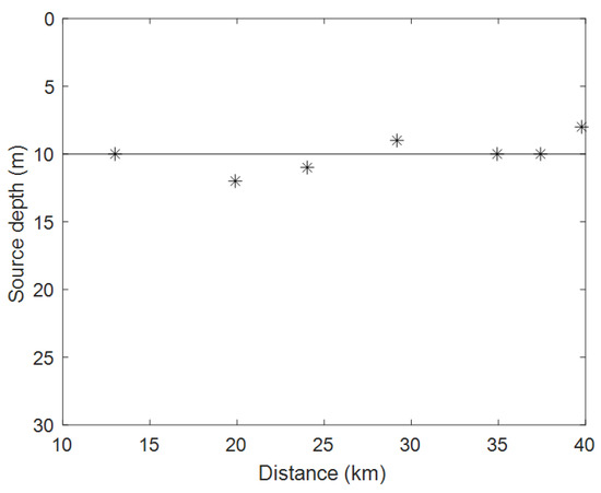
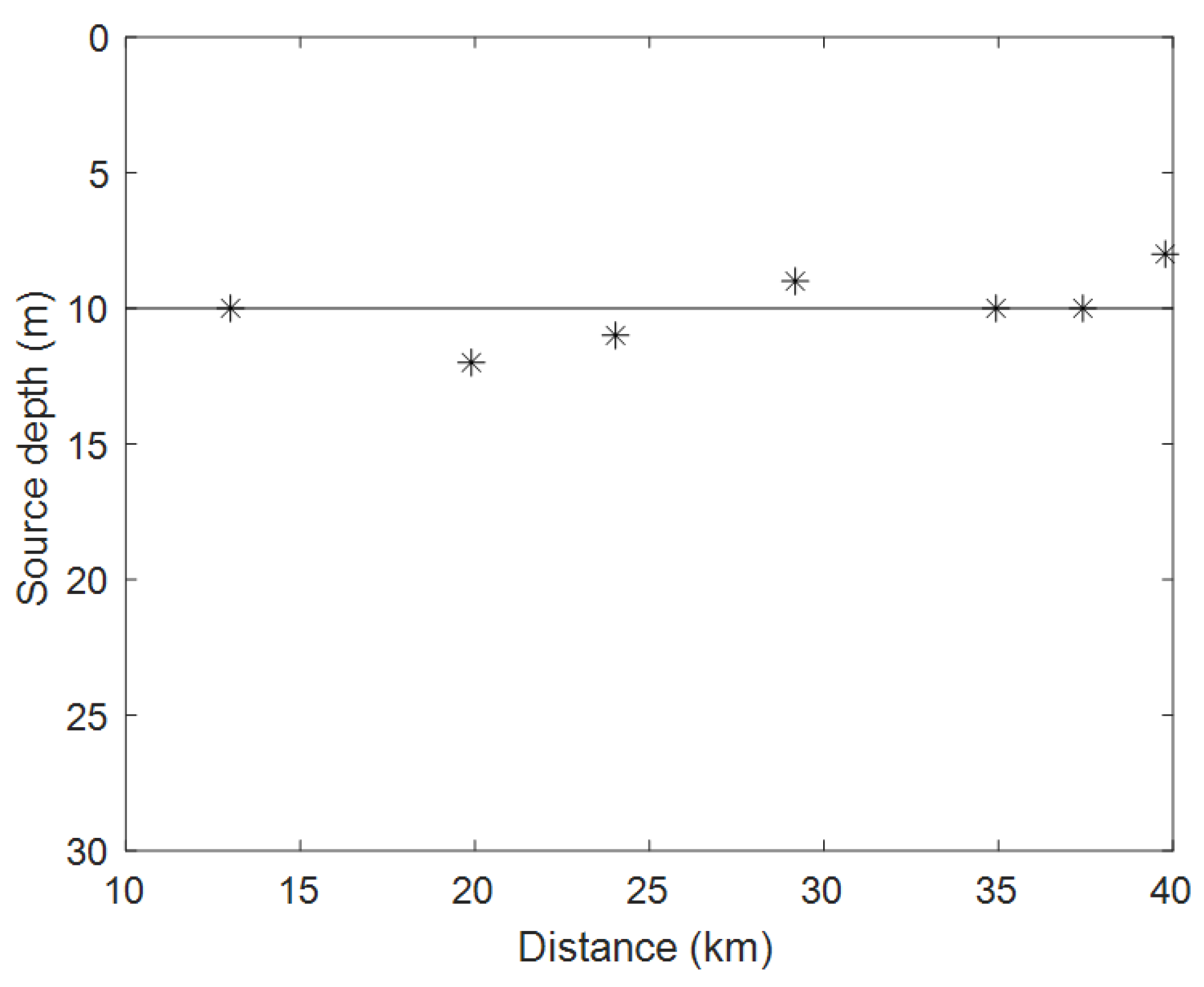
The results of depth estimation of multiple signals on this survey line are shown in Figure 16, and estimations can be seen to fluctuate in smaller magnitudes above and below 10 m. This is due to the swaying and heaving of the research vessel during the cruise in rough sea conditions.

Figure 16. Part of the depth estimation results for multiple shots along the survey line. Asterisks represent the estimated source depths, and the horizontal line indicates the nominal source depth of 10 m recorded in the experimental log. Fluctuations around 10 m are due to the swaying and heaving of the research vessel under rough sea conditions.

5. Discussion

Compared with existing shallow-water localization methods, the proposed method offers several key advantages: it does not require a guiding sound source with known distance, so it can directly estimate distance for non-cooperative objects. Furthermore, it requires fewer environmental parameters, depending primarily on the water depth and average sound speed. In addition, for the sloping seabed, the solution can be performed using Equation (18).

The essence of the proposed method is to use the relationship between the cut-off frequency of the normal mode in the shallow waveguide and the distance to the sound source, and to use the warping transform of the energy density function to obtain the EFs independent of the environmental parameters. The selection of the starting time of the warping transform is another issue to be considered. If the starting time of the warping transform does not coincide with the moment when the signal is reached, it will lead to a shift of the transformed EF position from the true value, making the distance estimation value have an obvious error. In this work, the starting time is determined by sweeping the time interval during which the normalized energy increases from 40% to 70% of its peak.

For depth estimation, the situation is different. Since the sound source depth estimation method utilizes the amplitude information of the EF, and when the distance estimation result is not accurate, both the frequency location and the amplitude of EFs will be distorted, as shown in Figure 3. Thus, distance estimation is not only the previous step in depth estimation, but its accuracy also affects the accuracy of depth estimation. In long-range scenarios, higher-order modes may become unobservable due to seabed attenuation and reduced SNR, resulting in fewer usable EFs than the theoretical maximum propagating mode order; how to determine the practically usable number of EFs remains a topic for future investigation. In addition, it is necessary to use the source signal and acoustic propagation model to generate a copy of the received acoustic signal, and then carry out the extraction of the EF peak ratio vector, so it is also necessary to consider the impact brought by the computational costs.

6. Conclusions

Passive source localization in shallow water has long been a challenging and extensively studied topic in underwater acoustics. In a shallow sea waveguide, the energy density function of the received signal of a single hydrophone contains the distance and depth information of the source in the frequency spectrum transformed by warping. The warped spectrum reveals EFs that are solely dependent on waveguide depth and average sound speed. Since the source range must be assumed during the warping transform, the discrepancy between the extracted and theoretical EF values can be exploited to rapidly estimate the true source range.

In this paper, the method was successfully extended to distance estimation in a sloping seabed environment, as demonstrated by the experimental results in Figure 14. When accurate distance estimation is obtained, there is a relationship between the energy of each order EF and the depth of the sound source. Then the amplitude matching method can be used to achieve the accurate estimation of the source depth. In this paper, the feasibility of the proposed method is verified by simulating and winter experiments, and the results of distance and depth estimation on one measurement line are given.

References

- Baggeroer, A.; Kuperman, W.; Mikhalevsky, P. An overview of matched field methods in ocean acoustics. IEEE J. Ocean. Eng. 1993, 18, 401–424. [Google Scholar] [CrossRef] [Scilit]
- Westwood, E.K. Broadband matched-field source localization. J. Acoust. Soc. Am. 1992, 91, 2777–2789. [Google Scholar] [CrossRef] [Scilit]
- Cockrell, K.L.; Schmidt, H. Robust passive range estimation using the waveguide invariant. J. Acoust. Soc. Am. 2010, 127, 2780–2789. [Google Scholar] [CrossRef] [Scilit] [PubMed]
- Bonnel, J.; Thode, A.; Wright, D.; Chapman, R. Nonlinear time-warping made simple: A step-by-step tutorial on underwater acoustic modal separation with a single hydrophone. J. Acoust. Soc. Am. 2020, 147, 1897–1926. [Google Scholar] [CrossRef] [Scilit] [PubMed]
- Bonnel, J.; Nicolas, B.; Mars, J.I.; Walker, S.C. Estimation of modal group velocities with a single receiver for geoacoustic inversion in shallow water. J. Acoust. Soc. Am. 2010, 128, 719–727. [Google Scholar] [CrossRef] [Scilit] [PubMed]
- Baggeroer, A.B.; Kuperman, W.A. Matched Field Processing in Ocean Acoustics. In Acoustic Signal Processing for Ocean Exploration; Moura, J.M.F., Lourtie, I.M.G., Eds.; Springer: Dordrecht, The Netherlands, 1993; pp. 79–114. [Google Scholar] [CrossRef] [Scilit]
- Chapman, N.R.; Shang, E.C. Review of Geoacoustic Inversion in Underwater Acoustics. J. Theor. Comput. Acoust. 2021, 29, 2130004. [Google Scholar] [CrossRef] [Scilit]
- Li, Q.-Q.; Yang, F.-L.; Zhang, K.; Zheng, B.-X. Moving source parameter estimation in an uncertain environment. Acta Phys. Sin. 2016, 65, 164304. [Google Scholar] [CrossRef] [Scilit]
- Qi, Y.B.; Zhou, S.H.; Zhang, R.H.; Ren, Y. A Waveguide-Invariant-Based Warping Operator and Its Application to Passive Source Range Estimation. J. Comput. Acoust. 2015, 23, 1550003. [Google Scholar] [CrossRef] [Scilit]
- Qi, Y.-B.; Zhou, S.-H.; Zhang, R.-H.; Ren, Y. A passive source ranging method using the waveguide-invariant-warping operator. Acta Phys. Sin. 2015, 64, 074301. [Google Scholar] [CrossRef] [Scilit]
- Byun, G.; Song, H.C.; Kim, J.S. Performance comparisons of array invariant and matched field processing using broadband ship noise and a tilted vertical array. J. Acoust. Soc. Am. 2018, 144, 3067–3074. [Google Scholar] [CrossRef] [Scilit] [PubMed]
- Song, H.C.; Byun, G. An overview of array invariant for source-range estimation in shallow water. J. Acoust. Soc. Am. 2022, 151, 2336–2352. [Google Scholar] [CrossRef] [Scilit] [PubMed]
- Potty, G.; Miller, J.; Dahl, P.; Lazauski, C. Geoacoustic Inversion Results from the ASIAEX East China Sea Experiment. IEEE J. Ocean. Eng. 2004, 29, 1000–1010. [Google Scholar] [CrossRef]
- Feng, S.; Zhu, X. A Transformer-Based Deep Learning Network for Underwater Acoustic Target Recognition. IEEE Geosci. Remote Sens. Lett. 2022, 19, 1505805. [Google Scholar] [CrossRef] [Scilit]
- Feng, S.; Zhu, X.; Ma, S. Masking Hierarchical Tokens for Underwater Acoustic Target Recognition with Self-Supervised Learning. IEEE/ACM Trans. Audio Speech Lang. Process. 2024, 32, 1365–1379. [Google Scholar] [CrossRef] [Scilit]
- Feng, S.; Ma, S.; Zhu, X. Graph Embedding with Mel-Spectrograms for Underwater Acoustic Target Recognition. IEEE J. Ocean. Eng. 2025, 51, 839–852. [Google Scholar] [CrossRef] [Scilit]
- Bonnel, J.; Thode, A. Using warping processing to range bowhead whale sounds from a single receiver. Proc. Mtgs. Acoust. 2013, 19, 070066. [Google Scholar] [CrossRef] [Scilit]
- Bonnel, J.; Dosso, S.E.; Ross Chapman, N. Bayesian geoacoustic inversion of single hydrophone light bulb data using warping dispersion analysis. J. Acoust. Soc. Am. 2013, 134, 120–130. [Google Scholar] [CrossRef] [Scilit] [PubMed]
- Wang, D.; Guo, L.-H.; Liu, J.-J.; Qi, Y.-B. Passive impulsive source range estimation based on warping operator in shallow water. Acta Phys. Sin. 2016, 65, 104302. [Google Scholar] [CrossRef] [Scilit]
- Guo, X.-L.; Yang, K.-D.; Ma, Y.-L.; Yang, Q.-L. A source range and depth estimation method based on modal dedispersion transform. Acta Phys. Sin. 2016, 65, 214302. [Google Scholar] [CrossRef] [Scilit]
- Li, X.-M.; Zhang, M.-H.; Zhang, H.-G.; Piao, S.-C.; Liu, Y.-Q.; Zhou, J.-B. A passive range method of broadband impulse source based on matched-mode processing. Acta Phys. Sin. 2017, 66, 094302. [Google Scholar] [CrossRef] [Scilit]
- Zhang, H.; Liu, W.; Zhang, L.; Meng, Y.; Han, W.; Song, T.; Yang, R. An allocation strategy integrated power, bandwidth, and subchannel in a RCC network. Def. Technol. 2026, 60, 138–154. [Google Scholar] [CrossRef] [Scilit]
- Jensen, F.B.; Kuperman, W.A.; Porter, M.B.; Schmidt, H. Computational Ocean Acoustics; Modern Acoustics and Signal Processing; Springer: New York, NY, USA, 2011. [Google Scholar] [CrossRef] [Scilit]
- Guo, X.-L.; Yang, K.-D.; Ma, Y.-L. A far distance wideband geoacoustic parameter inversion method based on a modal dispersion curve. Acta Phys. Sin. 2015, 64, 174302. [Google Scholar] [CrossRef] [Scilit]
- Qi, Y.-B.; Zhou, S.-H.; Zhang, R.-H.; Zhang, B.; Ren, Y. Modal characteristic frequency in a range-dependent shallow-water waveguide and its application to passive source range estimation. Acta Phys. Sin. 2014, 63, 044303. [Google Scholar] [CrossRef] [Scilit]
- Duan, R.; Ross Chapman, N.; Yang, K.; Ma, Y. Sequential inversion of modal data for sound attenuation in sediment at the New Jersey Shelf. J. Acoust. Soc. Am. 2016, 139, 70–84. [Google Scholar] [CrossRef] [Scilit] [PubMed]
- Guo, X.; Yang, K.; Duan, R.; Ma, Y. Sequential Inversion for Geoacoustic Parameters in the South China Sea Using Modal Dispersion Curves. Acoust. Aust. 2017, 45, 119–129. [Google Scholar] [CrossRef] [Scilit]
Disclaimer/Publisher’s Note: The statements, opinions and data contained in all publications are solely those of the individual author(s) and contributor(s) and not of MDPI and/or the editor(s). MDPI and/or the editor(s) disclaim responsibility for any injury to people or property resulting from any ideas, methods, instructions or products referred to in the content. |
© 2026 by the authors. Licensee MDPI, Basel, Switzerland. This article is an open access article distributed under the terms and conditions of the Creative Commons Attribution (CC BY) license.