Anti-Jamming GNSS Antenna Array Receiver with Reduced Phase Distortions Using a Robust Phase Compensation Technique

Abstract

Antenna arrays with adaptive filtering can protect the integrity and functionality of global navigation satellite system (GNSS) receivers against interference. However, a major problem with existing adaptive array processing algorithms is that they cause phase distortions and introduce bias errors into the carrier phase measurement, limiting high-precision applications. In this paper, a robust phase compensation technique is proposed to reduce the phase distortion. First, a phase bias detection method is developed to trigger the phase compensation technique. Then, the phase bias is estimated using a robust estimation method and compensated for in the GNSS receiver. The proposed technique operates in real time and causes no processing delay, while requiring only a minor modification to existing GNSS receivers. This technique is applied to the power inversion adaptive antenna, and can also be extended to a wide variety of adaptive antennas. The simulation experiments verify the applicability of the proposed technique and also confirm its superiority over existing techniques.

1. Introduction

The Global Navigation Satellite System (GNSS) is now widely used to provide position, velocity, and timing information in a wide variety of applications [1]. Unfortunately, the GNSS signal is easily disturbed by both intentional and unintentional interference [2]. Therefore, it is of great importance to keep GNSS receivers operating properly in environments containing interference. The adaptive antenna array is a state-of-the-art anti-jamming approach that can maintain the functionality of GNSS receivers in a harsh interference environment [1].

Blind anti-jamming algorithms, such as the power inversion (PI) algorithm [3], can suppress interference without any prior knowledge, making them popular in practical engineering [4]. However, apart from the problem of satellite signal attenuation [5], one of the main problems with these algorithms is that they cause phase distortions and introduce bias errors into the carrier phase [6]. The bias errors cannot be precalibrated since they vary in response to the operating environment [7]. Moreover, the biases vary from satellite to satellite [1], and can change significantly during interference suppression [8]. This measurement bias cannot be ignored, since it consequently results in a position deviation [9]. Therefore, maintaining high-precision measurement accuracy while suppressing interference is urgently needed.

To solve this problem, some researchers have attempted to optimize the array configuration. A special centrosymmetric array configuration that does not cause any phase distortion has been proposed [10,11]. However, this type of approach is not suitable when the nonideal factors of the array elements are taken into account. Moreover, sometimes, it is not easy to modify the array configuration in practice. Recently, a phase compensation technique was studied in the literature. The phase bias term is estimated and compensated for in this type of approach. The estimation of the phase bias can be divided into two approaches. The first approach is performed in the adaptive array processing. The phase-rotated steering vector of the satellite signal is estimated and used to obtain the phase bias estimate [12,13]. However, these methods significantly increase the computational complexity. Furthermore, the steering vector is estimated from its orthogonal component in the interference subspace. The accuracy of the estimates cannot be guaranteed and will therefore introduce biases. The second approach is accomplished in the receiver signal processing. The main advantage of this method is that it involves only the addition logic in the receiver, which does not require significant modifications to existing systems. The phase discriminator is used to obtain the phase bias estimate [14,15]. However, the estimation accuracy is easily affected by the phase discriminator noise. To address the above issues, the phase bias detection and estimation methods are investigated, and a robust phase compensation technique is proposed.

The remainder of this paper is organized as follows. Section 2 gives the signal model and formulates the problem. Section 3 presents the proposed phase compensation technique. Section 4 performs simulation experiments and analyzes the results. Finally, the conclusions are drawn in Section 5.

2. Signal Model and Problem Statement

This section first presents the signal model for GNSS receivers with an antenna array and analyzes the anti-jamming effect on the carrier phase. Then, the shortcomings of existing phase compensation techniques are briefly introduced.

2.1. Signal Model

The GNSS signal is received and downconverted by each antenna of a multisensor array, along with the interference and noise. The signals from all antenna elements can be combined into a vector as

$$\mathbf{x}\left(t\right)={\mathbf{a}}_{0}s\left(t\right)+\sum _{q=1}^Q{\mathbf{a}}_q{j}_q\left(t\right)+\mathbf{n}\left(t\right)$$

(1)

where t is the time, $\mathbf{x}\left(t\right)={[x_1\left(t\right),x_2\left(t\right),\dots ,x_N\left(t\right)]}^{\mathrm{T}}\in {\mathbb{C}}^{N\times 1}$ is the array snapshot with N being the number of antennas, $s\left(t\right)$ is the GNSS signal that is the signal of interest, $j_q\left(t\right)$ is the interfering signal transmitted from the q-th jammer, Q is the number of jammers, ${\mathbf{a}}_0\in {\mathbb{C}}^{N\times 1}$ and ${\mathbf{a}}_q\in {\mathbb{C}}^{N\times 1}$ are the steering vectors of $s\left(t\right)$ and $j_q\left(t\right)$, respectively, and $\mathbf{n}\left(t\right)\in {\mathbb{C}}^{N\times 1}$ is the additive noise vector. The GNSS signal, interfering signals, and noise are assumed to be mutually uncorrelated.

The GNSS signal in Equation (1) can be expressed as

$$s\left(t\right)=\sqrt{P}D(t-\tau )c(t-\tau ){\mathrm{e}}^{\mathrm{j}(2\pi (f_{\mathrm{IF}}+f_{\mathrm{d}})t+\phi )}$$

(2)

where P is the signal power, $D(·)$ is the navigation data bit, $c(·)$ is the pseudorandom noise code, $\tau$ is the signal delay, $f_{\mathrm{IF}}$ is the intermediate frequency, $f_{\mathrm{d}}$ is the Doppler frequency, and $\phi$ is the initial carrier phase.

To suppress the strong interference, the PI weight is calculated as [16]

$${\mathbf{w}}_{\mathrm{PI}}=\frac{{\mathbf{R}}_{xx}^{-1}\mathbf{b}}{{\mathbf{b}}^{\mathrm{H}}{\mathbf{R}}_{xx}^{-1}\mathbf{b}}$$

(3)

where ${\mathbf{R}}_{xx}=E\left[\mathbf{x}\left(t\right){\mathbf{x}}^{\mathrm{H}}\left(t\right)\right]$ denotes the autocorrelation matrix of the array input signal, $E[·]$ stands for the expectation operation, ${(·)}^{\mathrm{H}}$ denotes the conjugate transpose operation, and $\mathbf{b}={[1,0,\dots ,0]}^{\mathrm{T}}$ is a constraint vector.

Then, the output signal of the antenna array is obtained as

$$y_{\mathrm{PI}}\left(t\right)={\mathbf{w}}_{\mathrm{PI}}^{\mathrm{H}}\mathbf{x}\left(t\right)$$

(4)

2.2. Anti-Jamming Effect on the Carrier Phase

Substituting Equations (1) and (3) into Equation (4) yields

$$\begin{array}{cc}\hfill y_{\mathrm{PI}}\left(t\right)& =\frac{{\mathbf{b}}^{\mathrm{H}}{\mathbf{R}}_{xx}^{-1}{\mathbf{a}}_0}{{\mathbf{b}}^{\mathrm{H}}{\mathbf{R}}_{xx}^{-1}\mathbf{b}}s\left(t\right)+{\mathbf{w}}_{\mathrm{PI}}^{\mathrm{H}}\left[\sum _{q=1}^Q{\mathbf{a}}_q{j}_q\left(t\right)+\mathbf{n}\left(t\right)\right]\hfill \\ \hfill & =\alpha {\mathrm{e}}^{\mathrm{j}\psi }s\left(t\right)+n\left(t\right)\hfill \end{array}$$

(5)

where $\alpha$ and $\psi$ denote the scaling factor and the phase bias induced by the adaptive array, respectively. $n\left(t\right)$ represents the noise term after interference is effectively suppressed. Note that $\psi$ depends on the autocorrelation matrix ${\mathbf{R}}_{xx}$. Therefore, the phase bias varies when the operating environment changes.

The in-phase (I) and quadrature (Q) local carrier replicas are, respectively, generated by the numerically controlled oscillator (NCO) in the receiver as

$$\begin{array}{cc}\hfill i_{\mathrm{carr}}\left(t\right)& =cos(2\pi (f_{\mathrm{IF}}+{\widehat{f}}_{\mathrm{d}})t+\widehat{\phi })\hfill \\ \hfill q_{\mathrm{carr}}\left(t\right)& =-sin(2\pi (f_{\mathrm{IF}}+{\widehat{f}}_{\mathrm{d}})t+\widehat{\phi })\hfill \end{array}$$

(6)

where ${\widehat{f}}_{\mathrm{d}}$ is the local estimated Doppler frequency, and $\widehat{\phi }$ is the local estimated initial carrier phase.

The focus of this work is on carrier tracking, so it is assumed that the local code replica is synchronized with the received code. The array output in Equation (5) is correlated with the local signal replicas, and the I and Q correlation signals are obtained as

$$\begin{array}{cc}\hfill I& =A·D·sinc(\delta f·T)·cos(\pi \delta f·T+\delta \phi +\psi )+n_{\mathrm{I}}\hfill \\ \hfill Q& =A·D·sinc(\delta f·T)·sin(\pi \delta f·T+\delta \phi +\psi )+n_{\mathrm{Q}}\hfill \end{array}$$

(7)

where A is the correlation amplitude depending on the useful signal amplitude, D is the navigation data bit that is assumed to be constant over the integration time, $sinc\left(x\right)=sin\left(\pi x\right)/\pi x$, T is the coherent integration time, $\delta f=f_{\mathrm{d}}-{\widehat{f}}_{\mathrm{d}}$ is the Doppler frequency error, $\delta \phi =\phi -\widehat{\phi }$ is the initial phase error, and $n_{\mathrm{I}}$ and $n_{\mathrm{Q}}$ are correlation noise terms.

The two-quadrant arctangent phase discriminator can be used to obtain the phase error, and the discriminator output is given by

$$\delta \tilde{\phi }=arctan(Q/I)=(\pi \delta f·T+\delta \phi )+\psi +\xi$$

(8)

where $\xi$ denotes the discriminator noise, and the term enclosed in parentheses is the true phase error.

It can be seen from Equation (8) that the phase bias is induced into the discriminator output and this can be viewed as the phase step input [17]. The steady-state error of the phase-locked loop is zero under this circumstance [17], i.e., $\widehat{\phi }=\phi +\psi$ at steady state. This indicates that the phase bias is eventually introduced into the GNSS carrier phase measurement, resulting in a significant phase discontinuity.

2.3. Existing Phase Compensation Techniques

To solve the above problem, a kind of phase compensation technique was developed in [14,15]. In these works, the local carrier replica is assumed to be aligned with $s\left(t\right)$, i.e., $\delta f=0$ and $\delta \phi =0$, and the correlation noise is ignored. Thus, the discriminator output can be obtained as $\delta \tilde{\phi }=arctan(Q/I)=\psi$.

The phase bias estimation is performed by directly using the discriminator output as the phase bias estimate, given by

$$\widehat{\psi }=\delta \tilde{\phi }$$

(9)

Then, the phase compensation is performed by adjusting the NCO using the phase bias estimate to obtain the modified local carrier replicas as

$$\begin{array}{cc}\hfill {\widehat{i}}_{\mathrm{carr}}\left(t\right)& =cos(2\pi (f_{\mathrm{IF}}+{\widehat{f}}_{\mathrm{d}})t+\widehat{\phi }+\widehat{\psi })\hfill \\ \hfill {\widehat{q}}_{\mathrm{carr}}\left(t\right)& =-sin(2\pi (f_{\mathrm{IF}}+{\widehat{f}}_{\mathrm{d}})t+\widehat{\phi }+\widehat{\psi })\hfill \end{array}$$

(10)

Therefore, if $\widehat{\psi }=\psi$, the phase bias disappears from the I and Q correlation signals in Equation (7). Thus, the carrier phase estimate $\widehat{\phi }$ is not affected.

There are two problems that hinder the use of this type of phase compensation technique in practical applications. (1) The existing phase compensation technique lacks phase bias detection. In the existing phase compensation technique, the correlation noise is ignored and it is considered that if $\widehat{\psi }\ne 0$, then the phase bias appears. However, in practice, the correlation noise is unavoidable, which makes it difficult to determine the phase bias appearance time. (2) The existing phase compensation technique has poor phase bias estimation. This is because the discriminator output is directly used as the phase bias estimate, and it cannot mitigate the random noise and gross errors. This problem is especially severe if the satellite signal is not strong enough.

3. Proposed Technique

This section describes the proposed technique, which consists of two main parts, including phase bias detection and phase bias estimation.

3.1. Phase Bias Detection

This subsection first gives the reason for the phase bias detection, then the detection method is presented.

The dynamic behavior of the NCO can be characterized by a state vector ${\mathbf{X}}_k={[{\phi }_k,{\omega }_k,{\dot{\omega }}_k]}^{\mathrm{T}}$, with the corresponding parameters being initial carrier phase ${\phi }_k$, angular Doppler frequency ${\omega }_k$, and angular Doppler frequency rate of change ${\dot{\omega }}_k$ at the k-th time epoch, and ${[·]}^{\mathrm{T}}$ denotes the transpose operation.

The NCO can be tuned by the prediction model, and the locally predicted NCO is obtained as

$${\widehat{\mathbf{X}}}_k^{-}=\mathbf{F}{\widehat{\mathbf{X}}}_{k-1}+\mathbf{B}{\mathbf{u}}_{k-1}$$

(11)

where $\mathbf{B}={[T,0,0]}^{\mathrm{T}}$, ${\mathbf{u}}_k=f_{\mathrm{IF}}$, and $\mathbf{F}$ has the form

$$\mathbf{F}=\left[\begin{array}{ccc}1& T& T^2/2\\ 0& 1& T\\ 0& 0& 1\end{array}\right]$$

(12)

The discriminator output in Equation (8) is used to adjust the NCO prediction as

$${\widehat{\mathbf{X}}}_k={\widehat{\mathbf{X}}}_k^{-}+{\mathbf{K}}_k\delta {\tilde{\phi }}_k$$

(13)

where ${\mathbf{K}}_k$ denotes the loop gain, which can be determined by the conventional tracking loop design or the Kalman filter approach [18]. In this work, the latter is used to obtain reasonable tracking performance.

When the discriminator output is contaminated by the phase bias, as seen in Equation (8), it will therefore misadjust the NCO through Equation (13). If the induced phase bias can be detected, the negative effect can be cut off immediately, so two indicators for phase bias detection are designed below.

Monitoring the change of interference conditions is an effective method for phase bias detection. Therefore, the interference cancellation ratio (ICR) [19] can be adopted, which is approximately calculated as

$$\mathrm{ICR}=\frac{P_{\mathrm{in}}}{P_{\mathrm{out}}}$$

(14)

where $P_{\mathrm{in}}$ and $P_{\mathrm{out}}$ are the array input and output power, respectively. It should be pointed out that the interference is assumed to be stable and far enough away from the target receiver. That is, it is assumed that the jamming power does not vary over the receiver operating time. The ICR can then be used to monitor changes as the jammer appears or disappears.

As a complement, the phase of weight (POW) can also reflect the change in array-induced phase bias, which is defined by the array weight as

$$\mathrm{POW}=\angle \left[\sum _{n=1}^N{w}_n^{*}\right]$$

(15)

where ∠ denotes the phase of a complex scalar, $w_n$ is the n-th element of the array weight, and ${(·)}^{*}$ denotes the complex conjugate. The POW actually represents a specific phase bias when the GNSS signal arrives perpendicular to the array plane, since, in this case, the satellite steering vector is an all-one column. The POW can then be used to monitor changes as the interference direction varies.

Note that both the ICR and the POW are obtained from the adaptive array, which is not affected by the receiver itself. In order to locate the time when the phase bias appears, the first-order differential method can be easily applied to these two indicators to obtain

$$d_{\mathrm{ICR}}=|\mathrm{ICR}\left(k\right)-\mathrm{ICR}(k-1)|>T_{\mathrm{I}}$$

(16)

$$d_{\mathrm{POW}}=|\mathrm{POW}\left(k\right)-\mathrm{POW}(k-1)|>T_{\mathrm{P}}$$

(17)

where $d_{\mathrm{ICR}}$ and $d_{\mathrm{POW}}$ denote the detection statistics, with $T_{\mathrm{I}}$ and $T_{\mathrm{P}}$ being the corresponding predefined thresholds, which are empirically set to 3 dB and 8 degrees, respectively. k and $k-1$ are the current and previous time epochs, respectively.

Further discussions about the detection proceed as follows. The detection thresholds are chosen based on experience because it is not easy to determine the specific value based on the detection probability for a given false alarm probability. A higher threshold may result in missed detection, while a lower threshold may result in false alarms that cause compensation to be triggered frequently, increasing the risk of the tracking loop losing lock. The recommended principle is to set a relatively high threshold to reduce false alarms. Based on our testing, the above thresholds work well in most situations. To increase the detection probability, the designed indicators can also be extended to combine more advanced techniques, such as interference direction estimation and interference source localization. More details are beyond the scope of this paper.

3.2. Phase Bias Estimation

This subsection deals with the estimation issue of the unknown phase bias term, allowing the undesired phase bias to be compensated for.

Recalling Equation (5), it is clear that the phase bias can be calculated if the array weight and the satellite steering vector are known. The former is easily obtained from the adaptive array, but the latter is not. Although the satellite direction can be determined from the ephemeris, obtaining the satellite steering vector also requires accurate knowledge of the array manifold and the array attitude. In order to obtain a self-contained phase bias estimate, a phase bias estimation approach is developed below.

The estimation of the phase bias is divided into two cases, including the jammer present and absent cases. The ICR in Equation (14) can be used as a judgment condition. If the following condition is found, the jammer is considered to be absent, and vice versa.

$$\mathrm{ICR}<T_{\mathrm{J}}$$

(18)

where $T_{\mathrm{J}}$ is a predefined threshold that can be set to 3 dB.

If the jammer is not present, because the satellite signal is much weaker than the noise, ${\mathbf{R}}_{xx}\approx {\sigma }_n^2\mathbf{I}$, where ${\sigma }_n^2$ is the noise power, and $\mathbf{I}$ denotes the identity matrix. In this case, it can be considered that no phase bias has been introduced, so the phase bias estimate is $\widehat{\psi }=0$. If the jammer is present, the phase bias is estimated as follows.

Suppose that the phase bias is detected at the K-th correlation epoch, then in the successive correlation epochs of window size L, i.e., $[K,K+L-1]$ correlation epochs, the NCO is tuned using ${\widehat{\mathbf{X}}}_k^{-}$, excluding $\delta {\tilde{\phi }}_k$ contaminated by the phase bias.

Assume that the signal dynamics do not change dramatically and that the phase bias value does not change in these L epochs, since it is at the millisecond level. Thus, the local carrier replica matches $s\left(t\right)$ well, i.e., $\delta f\approx 0$ and $\delta \phi \approx 0$. Therefore, the discriminator output in Equation (8) can be written as

$$\delta {\tilde{\phi }}_k\approx \psi +{\xi }_k$$

(19)

Then, the linear observation function with respect to the unknown phase bias can be written in matrix form as

$$\mathbf{z}=\mathbf{A}\psi +\Delta$$

(20)

where $\mathbf{z}={[\delta {\tilde{\phi }}_K,\delta {\tilde{\phi }}_{K+1},\dots ,\delta {\tilde{\phi }}_{K+L-1}]}^{\mathrm{T}}$ is an L-dimensional independent observation sequence, $\mathbf{A}$ is an L-dimensional all-one observation column vector, and $\Delta$ is the L-dimensional observation error vector.

The corresponding error function of Equation (20) can be expressed as

$$\mathbf{v}=\mathbf{A}\widehat{\psi }-\mathbf{z}$$

(21)

where $\mathbf{v}$ denotes the observation residual vector.

Thus, based on the robust estimation theory [20], the estimate can be obtained by the following criterion:

$$\sum _{i=1}^L\rho \left(v_i\right)=\min$$

(22)

where $v_i$ denotes the i-th element of $\mathbf{v}$, and $\rho (·)$ is a bounded convex function used to attenuate the effect of observation outliers. Then the iterative form of the solution can be expressed as

$$\left\{\begin{array}{c}{\widehat{\psi }}^{(j+1)}={\left({\mathbf{A}}^{\mathrm{T}}{\overline{\mathbf{P}}}^{\left(j\right)}\mathbf{A}\right)}^{-1}{\mathbf{A}}^{\mathrm{T}}{\overline{\mathbf{P}}}^{\left(j\right)}\mathbf{z}\hfill \\ {\mathbf{v}}^{(j+1)}=\mathbf{A}{\widehat{\psi }}^{(j+1)}-\mathbf{z}\hfill \end{array}\right.$$

(23)

where ${\overline{\mathbf{P}}}^{\left(j\right)}$ denotes the equivalent weight matrix of the observation vector at the j-th iteration. In the independent case, $\overline{\mathbf{P}}$ is a diagonal matrix. The form of the equivalent weight matrix is determined by $\rho (·)$, and the IGG-III weight function is a good choice, given by [21]:

$${\overline{P}}_i=\left\{\begin{array}{cc}{P}_i,\hfill & |{\overline{v}}_i|\le c_0\hfill \\ P_i\frac{c_0}{|{\overline{v}}_i|}{\left(\frac{c_1-|{\overline{v}}_i|}{c_1-c_0}\right)}^2,\hfill & c_0<\left|{\overline{v}}_i\right|\le c_1\hfill \\ 0,\hfill & |{\overline{v}}_i|>c_1\hfill \end{array}\right.$$

(24)

where ${\overline{P}}_i$ is the i-th diagonal of the equivalent weight matrix, $P_i$ is the i-th diagonal of the original weight matrix, ${\overline{v}}_i$ is the standardized residual expressed as ${\overline{v}}_i=v_i/{\sigma }_{v_i}$, and ${\sigma }_{v_i}$ is the standard deviation of $v_i$. ${\overline{P}}_i$ is a descending function with respect to the standardized residual, so that the effect of observation outliers can be reduced. $c_0$ and $c_1$ are the detection thresholds, which are generally taken as $c_0=1.0$–1.5 and $c_1=2.5$–8.0, respectively.

It is worth noting that if $\rho (·)$ is chosen as the quadratic cost function, and the weight matrix is selected as the identity matrix, then the solution of Equation (22) is the averaging estimation, i.e., $\widehat{\psi }=\frac{1}{L}{\sum }_{l=1}^L\delta {\tilde{\phi }}_{K+L-l}$. This solution is intuitive but has no rejection capability for the observation outliers, as shown in the following simulations.

It should also be noted that there is a trade-off in the selection of the window size L. That is, increasing L has the advantage of attenuating the discriminator noise, which may result in a better phase bias estimate. However, it also increases the prediction error and the risk of tracking loop divergence.

3.3. Implementation of the Proposed Technique

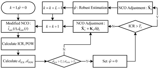
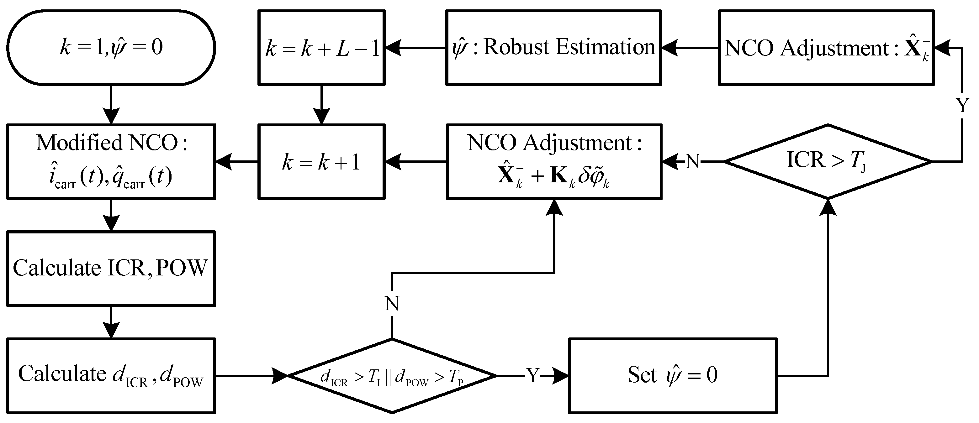
The proposed technique is obtained by combining the two parts in the previous subsections. The flowchart of the proposed technique is shown in Figure 1 with detailed steps summarized as follows.

Figure 1. Flowchart of the proposed technique.

(1)

The initialization parameters are set to $k=1$ and $\widehat{\psi }=0$. The array output signal is obtained using Equation (4) and the local carrier replica is generated as Equation (10).

(2)

The ICR and POW can be calculated according to Equations (14) and (15), and the $d_{\mathrm{ICR}}$ and $d_{\mathrm{POW}}$ can be obtained through Equations (16) and (17).

(3)

If $d_{\mathrm{ICR}}>T_{\mathrm{I}}\left|\right|d_{\mathrm{POW}}>T_{\mathrm{P}}$ at the K-th correlation epoch, then the phase bias estimate is reset to $\widehat{\psi }=0$ to start phase bias estimation. Otherwise, move to step (5).

(4)

If $\mathrm{ICR}>T_{\mathrm{J}}$, then the NCO is tuned by the prediction model using ${\widehat{\mathbf{X}}}_k^{-}$ (see Equation (11)) in $[K,K+L-1]$ correlation epochs. The phase bias is estimated using robust estimation in Equations (19)–(24). After that, set $k=k+L-1$, and move to step (6). Otherwise, move to step (5).

(5)

The NCO is tuned using ${\widehat{\mathbf{X}}}_k={\widehat{\mathbf{X}}}_k^{-}+{\mathbf{K}}_k\delta {\tilde{\phi }}_k$ in Equation (13).

(6)

Set $k=k+1$ and return to step (2).

From the above, it can be seen that the proposed technique inserts the phase bias detection and estimation processing (steps (2)–(4)) into the conventional receiver processing (steps (1), (5), and (6)). The proposed technique operates in real time, with no processing delays, and requires only modest changes to existing receivers.

4. Simulation Experiments

This section carries out several simulation experiments to verify the performance of the proposed technique and compare it with existing techniques.

4.1. Parameter Estimation Performance Analysis

In this subsection, the parameter estimation performance for phase biases is evaluated through Monte Carlo simulations. As described earlier in Equation (19), the phase bias can be considered as a constant, and the estimation is obtained by observing it in a noisy environment. Several estimation methods are carried out and compared below.

It has been mentioned that the existing phase compensation technique uses one observation directly as an estimate. This is referred to as the single point estimation in this paper. The robust estimation approach proposed in Section 3.2 obtains the estimate using a window size of L observation sequence. In this simulation, L is set to 30 for illustration. The averaging estimation is also considered in this simulation.

To compare the three estimation methods mentioned above under different observation conditions, the noise term in Equation (19) is considered as Gaussian and non-Gaussian distributions, which can be modeled as follows:

(1)

Gaussian condition:

$${\xi }_k\sim \mathcal{N}(0,R)$$

(25)

(2)

Non-Gaussian condition:

$${\xi }_k\sim \left\{\begin{array}{cc}\mathcal{N}(0,R),\hfill & \mathrm{w}.\mathrm{p}.0.9\hfill \\ \mathcal{N}(0,100R),\hfill & \mathrm{w}.\mathrm{p}.0.1\hfill \end{array}\right.$$

(26)

where $\mathcal{N}(\mu ,\Sigma )$ denotes the Gaussian probability density function with mean $\mu$ and variance $\Sigma$, w.p. means “with probability”, and R denotes the nominal observation noise variance. When the arctangent discriminator is used, the noise variance can be calculated as [18]

$$R={\sigma }_{\xi }^2=\frac{1}{2T·C/N_0}\left(1+\frac{1}{2T·C/N_0}\right)$$

(27)

where $C/N_0$ denotes the the carrier-to-noise ratio. In this simulation, the coherent integration time is set to $T=1\mathrm{ms}$.

The non-Gaussian condition in Equation (26) is an outlier corrupted condition since ten percent of the observation noise values are drawn from the Gaussian distribution with severely increased variance. This condition can be used to test the robustness of the estimation methods. Note that a good estimation method should not be significantly disturbed by the potential observation outliers.

The root mean square error (RMSE) is chosen as the performance metric, which is defined as

$$\mathrm{RMSE}\triangleq \sqrt{\frac{1}{M}\sum _{m=1}^M{(\psi -{\widehat{\psi }}^{\left(m\right)})}^2}$$

(28)

where $\psi$ is the real phase bias value, ${\widehat{\psi }}^{\left(m\right)}$ is the estimated phase bias value at the m-th Monte Carlo run, and M = 10,000 represents the total number of Monte Carlo runs.

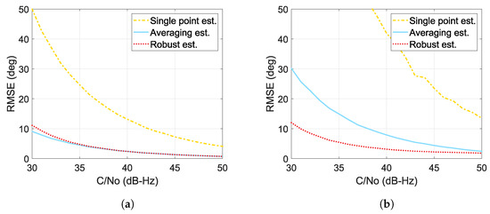
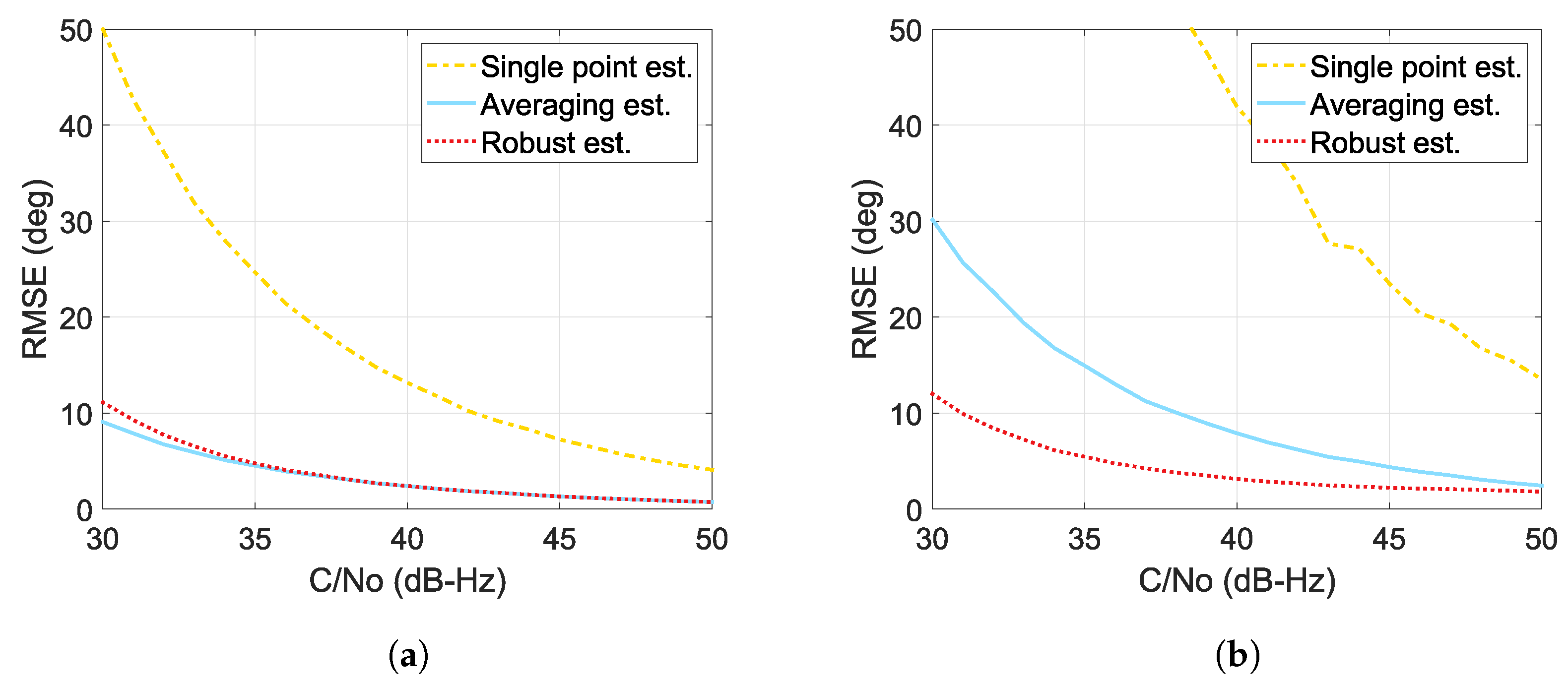
Figure 2 shows the RMSE results obtained by different estimation methods in association with different signal strengths under the Gaussian and non-Gaussian conditions. It can be seen that the RMSE decreases as the $C/N_0$ increases. However, the estimation accuracy of these estimation methods varies. It is shown that the single point estimation performs worst in both the Gaussian and non-Gaussian conditions, as expected. This is because this estimation approach cannot eliminate the effect of random noise and gross errors.

Figure 2. RMSE results using different estimation methods at different $C/N_0$ conditions. (a) Gaussian condition. (b) Non-Gaussian condition.

From Figure 2a, the averaging estimation achieves the most accurate estimation in the Gaussian condition, as it is the optimal estimation under this circumstance. The robust estimation sacrifices a little accuracy for robustness. When $C/N_0$ is 30–35 dB-Hz, the accuracy of the robust estimation is relatively lower than that of the averaging estimation. However, it is not easy to track such a weak signal when $T=1\mathrm{ms}$. Therefore, the accuracy of the phase bias estimation is not important in this case. From Figure 2b, it is shown that the robust estimation has the best estimation accuracy under the non-Gaussian condition, indicating that it has excellent robustness resistant to observation outliers.

Comparing Figure 2a and Figure 2b, it can be seen that the single point estimation is significantly affected since only one observation is used, resulting in nontolerable estimation errors. It can also be seen that the averaging estimation is also obviously influenced, as it has no outlier rejection capability. The presence of outliers in the non-Gaussian condition significantly deteriorates the estimation of the averaging approach. In contrast, the robust estimation shows its robustness under the non-Gaussian condition, and its performance is rarely affected. This is because it uses a descending weighting function to reduce the influence of abnormal outliers, as discussed in Section 3.2.

The simulation results verify that the robust estimation has a good balance between accuracy and robustness. Since a good phase bias estimation capability is essential for phase compensation, the robust estimation is expected to provide the expected phase compensation performance in the proposed technique.

4.2. Simulation Model and Parameter Settings

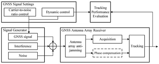
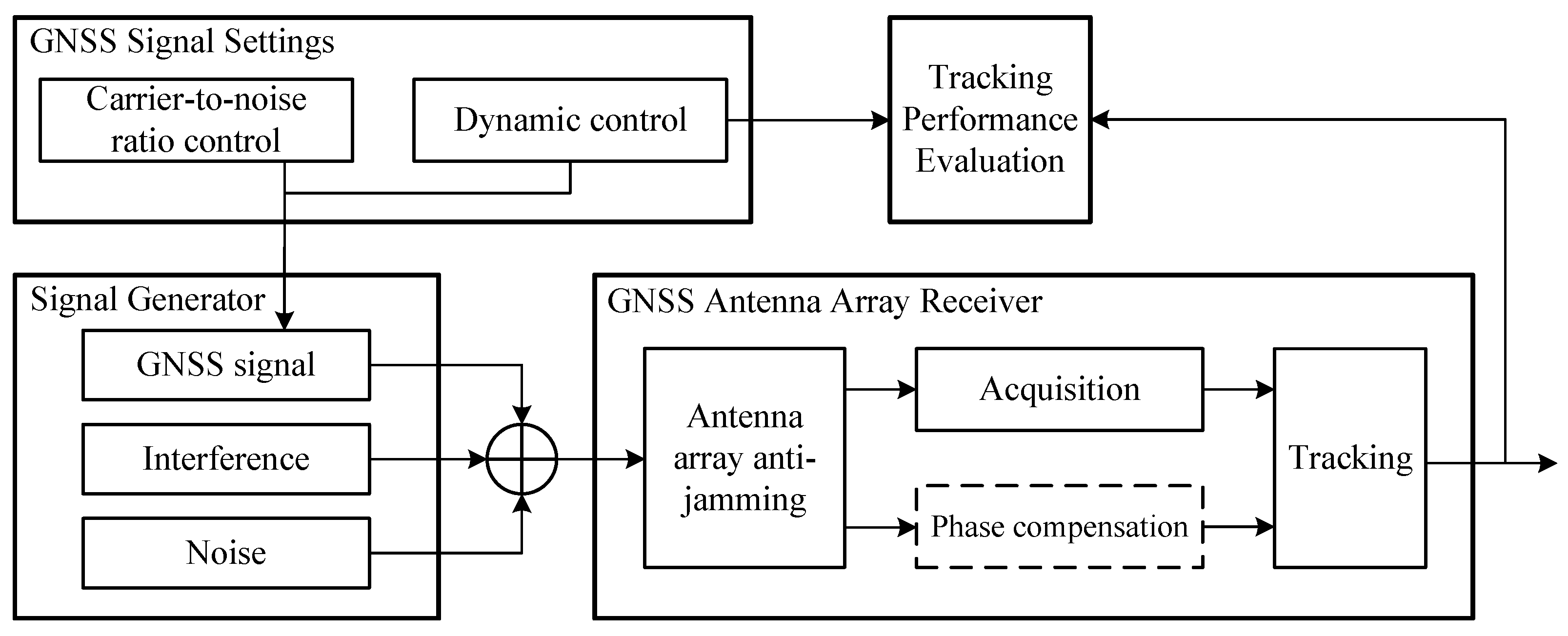
The performance of the proposed technique is tested using the simulation model shown in Figure 3. The simulation model consists of four modules, which are introduced as follows. The GNSS signal settings module is used to determine the $C/N_0$ and the dynamics of the GNSS signal. The compound signal received by the antenna array is produced in the signal generator module by adding the GNSS signal, interference, and noise. The compound signal is sent to the GNSS antenna array receiver module for processing. The tracking performance evaluation module is used to analyze the tracking error of the receiver.

Figure 3. Block diagram of the simulation model.

A four-element circular array with three equally spaced elements at half wavelength and a central element is chosen for performance validation. The GPS L1 C/A signal is considered as the signal of interest. The dynamics of the GNSS signal are assumed to have a constant Doppler frequency unless otherwise specified. A broadband (BB) interfering signal and a continuous wave (CW) interfering signal are injected from different directions at $t=0.5\mathrm{s}$ and $t=1.2\mathrm{s}$, respectively. In addition to the situation where new jammers appear, the situation where existing jammers disappear from the scene is also considered. The BB and CW interfering signals disappear at $t=1.8\mathrm{s}$ and $t=2.5\mathrm{s}$, respectively. The parameters used in the simulations are listed in Table 1.

Table 1. Parameters used in the simulations.

Parameter	Value
GNSS signal $C/N_0$	40 dB-Hz
GNSS elevation angle	75 deg
GNSS azimuth angle	200 deg
BB interference-to-noise ratio	40 dB
BB elevation angle	15 deg
BB azimuth angle	60 deg
CW interference-to-noise ratio	50 dB
CW elevation angle	10 deg
CW azimuth angle	150 deg

The existing phase compensation technique cannot be applied directly, and it is inserted into the architecture of the proposed technique for comparison. In this technique, the discriminator output is directly used as the phase bias estimate as described in Section 2.3. This technique is named the simple phase compensation (SPC) technique. The proposed technique is referred to as the robust phase compensation (RPC) technique. The PI algorithm is used for interference suppression. The adaptive array weight is calculated using the sample matrix inversion technique and is updated every 1 ms. The coherent integration time is set to 1 ms. The window size L for the RPC is set to 30.

4.3. Effectiveness of the Proposed Technique

In this subsection, the effectiveness of the proposed technique is verified. First, the performance of the phase bias detection is validated. Then, the carrier tracking performance is focused on. For comparison, the RPC with averaging estimation and the RPC with robust estimation are both considered. They are denoted in the figures by the legends “RPC, AE” and “RPC, RE”, respectively. Note that the results without phase compensation are denoted by the legend “Original”.

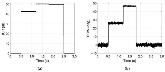
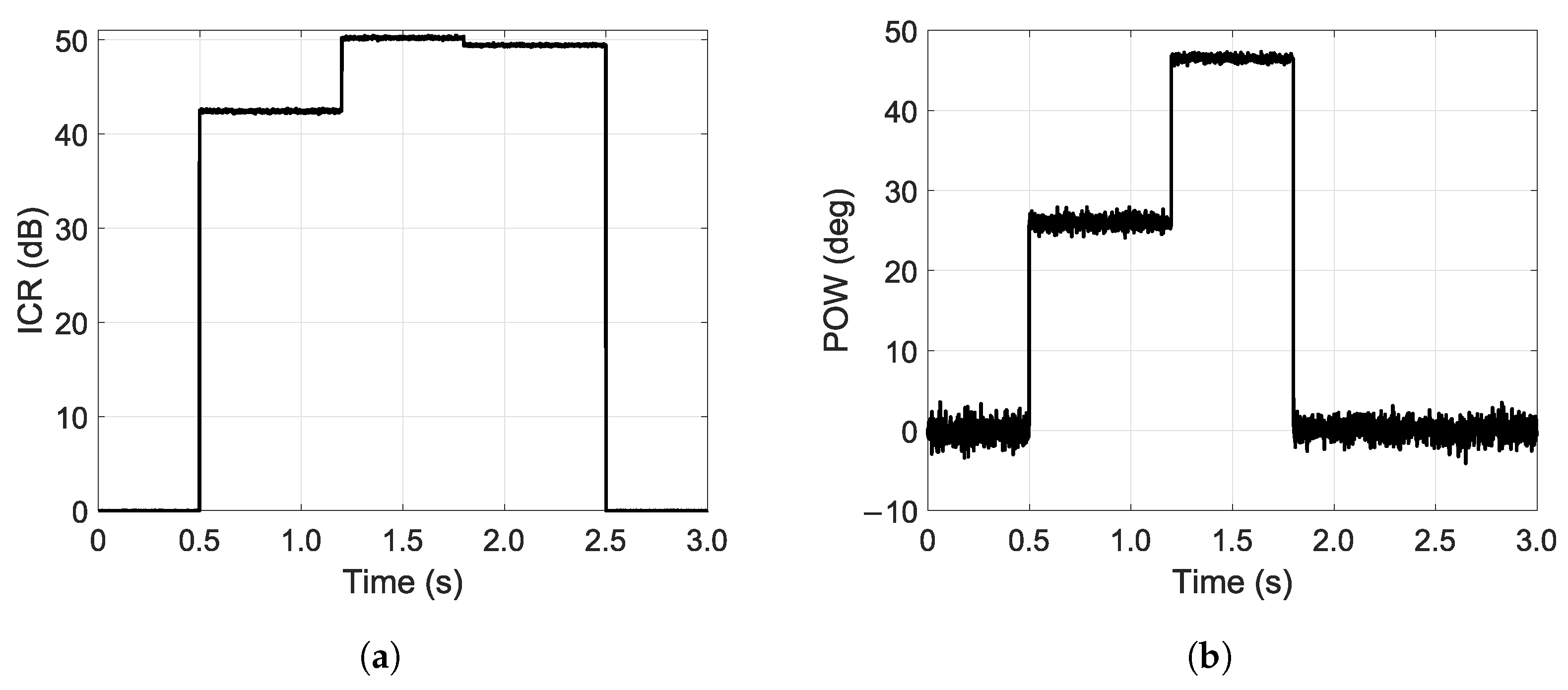
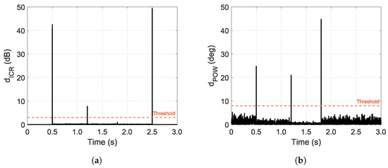
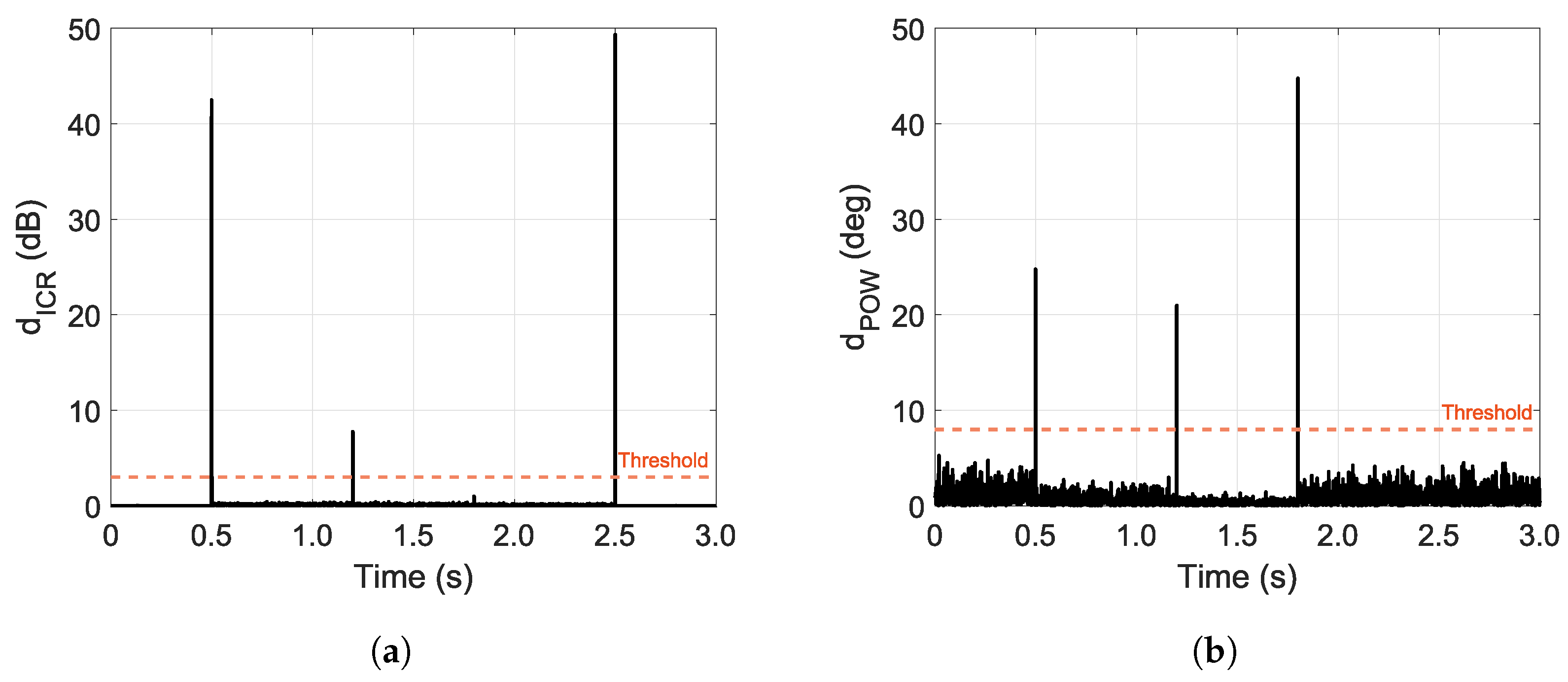
Figure 4 and Figure 5 show the designed indicators and the corresponding phase bias detection statistics, respectively. From Figure 4, it can be seen that the ICR is close to zero when there is no jammer; otherwise, it becomes extremely large, indicating that the interference is being mitigated. Moreover, when the jamming environment changes, significant changes in the ICR and POW occur immediately, indicating that a new phase bias is induced. It can also be seen from Figure 5 that the designed indicators are suitable for phase bias detection by setting appropriate thresholds. It should also be noted that these two detection statistics are complementary. Taking the complement of the two allows the phase bias appearance time to be fully located. This alerts the phase compensation techniques to start.

Figure 4. Designed indicators for phase bias detection. (a) ICR. (b) POW.

Figure 5. Phase bias detection statistics. (a) $d_{\mathrm{ICR}}$. (b) $d_{\mathrm{POW}}$.

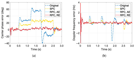
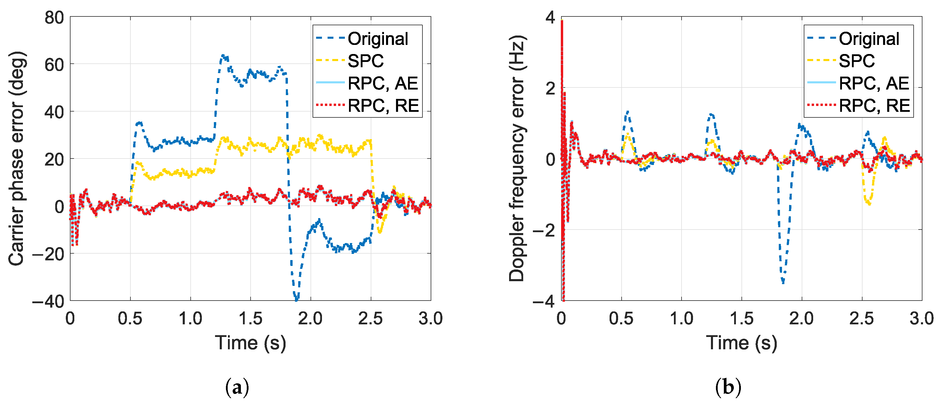
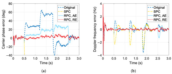
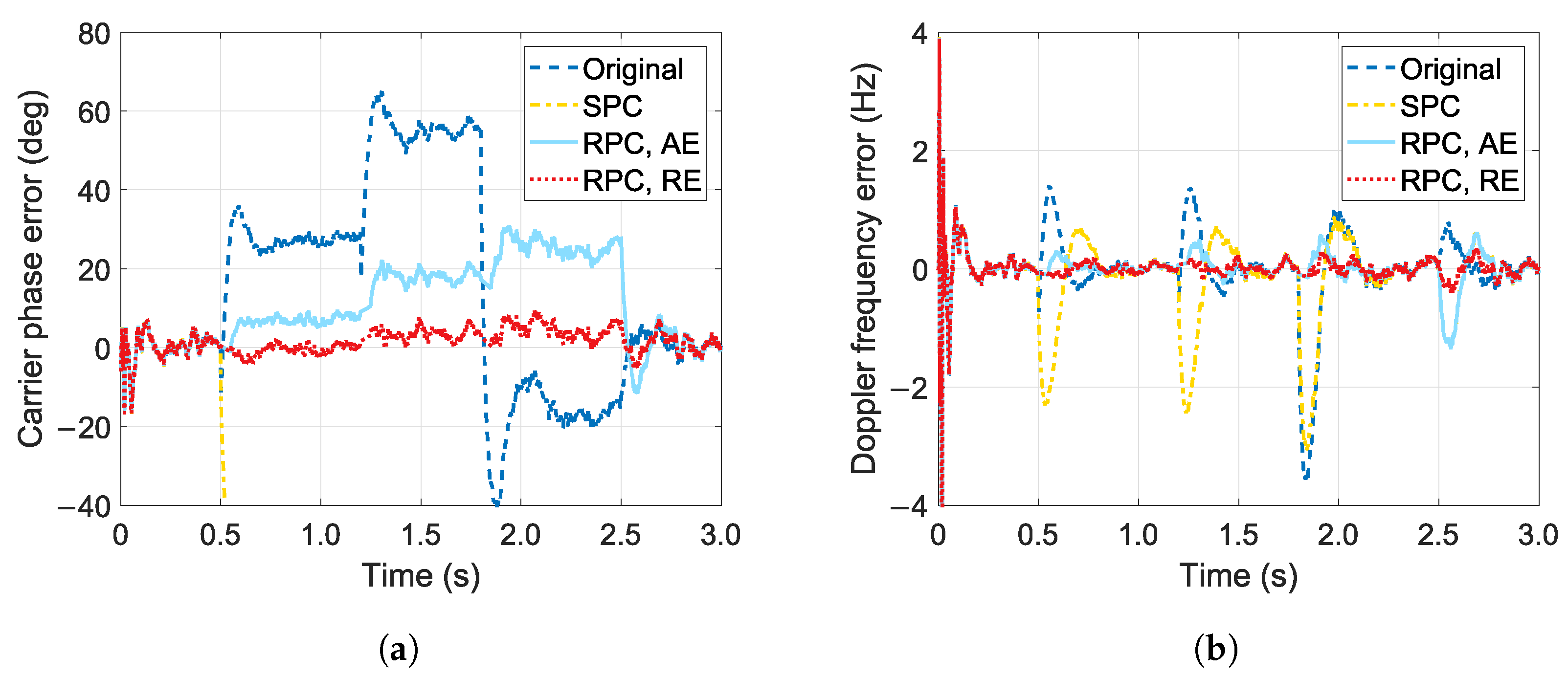
Figure 6 shows the carrier tracking errors with and without phase compensation techniques. From Figure 6a, it is clear that the PI algorithm without phase compensation techniques introduces significant biases into the carrier phase measurement. The carrier phase measurement accuracy is sacrificed for the purpose of interference mitigation. It can also be noted that the SPC can reduce the phase distortions to some extent, but its performance is limited due to poor phase bias estimation. The RPCs compensate for most phase biases and provide the best carrier phase accuracy. Moreover, when there are no outliers in the observation window, the RPC with averaging estimation and the RPC with robust estimation achieve similar phase bias estimation and compensation performance. This result is in agreement with that in Section 4.1. It can also be seen from Figure 6b that when the phase bias appears, the Doppler frequency jumps accordingly and then converges to the unbiased steady state. The use of phase compensation techniques can reduce the Doppler frequency errors during the transient state, thereby improving the Doppler frequency accuracy.

Figure 6. Carrier tracking errors with and without phase compensation techniques. (a) Carrier phase error. (b) Doppler frequency error.

4.4. Robustness of the Proposed Technique

To verify the robustness of the proposed technique, an outlier contaminated case is generated based on the simulation in the previous subsection. Three consecutive outliers are added to the discriminator output after the jamming environment changes, while other simulation parameters remain the same. This means that ten percent of the observations in the window are contaminated by outliers for the RPCs, which is the case in Section 4.1.

Figure 7 shows the carrier tracking errors with and without phase compensation techniques under the outlier contaminated case. A comparison of Figure 6 and Figure 7 reveals the following. (1) From the original curves in the two figures, it is known that several outliers in the discriminator output do not significantly affect the tracking results because the duration of the outliers is not long enough. (2) Comparing the SPC curves in the two figures, it is verified that the performance of the SPC is poor because its phase bias estimation is easily destroyed by outliers. (3) The performance of the RPC with averaging estimation is severely degraded by the outliers in the observation window due to the lack of outlier rejection capability. (4) The RPC with robust estimation shows its robustness to observation outliers and maintains high-precision carrier measurement accuracy under this severe condition. The results (2)–(4) agree with those in Section 4.1, and also validate the robustness of the proposed technique.

Figure 7. Carrier tracking errors with and without phase compensation techniques under the outlier contaminated case. (a) Carrier phase error. (b) Doppler frequency error.

4.5. Applicability of the Proposed Technique

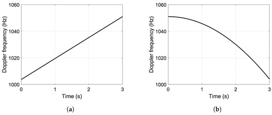
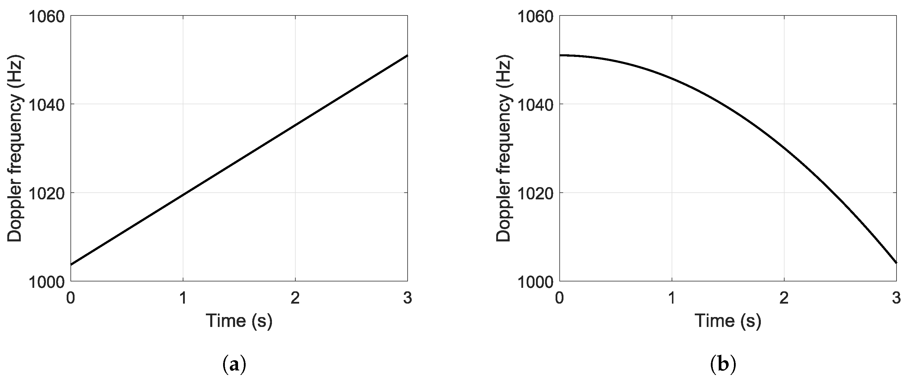
This subsection verifies the applicability of the proposed technique while considering only the RPC with robust estimation. In the previous simulations, the GNSS signal is assumed to have a constant Doppler frequency, which is not realistic in practice. Therefore, the GNSS signal is modified using the GNSS signal settings module in Figure 3 to test different conditions. Two types of common GNSS signal dynamics are considered, including uniform acceleration dynamics (denoted as Acc dynamics) and sinusoidal acceleration dynamics (denoted as Sin dynamics). These two types of GNSS signal dynamics are shown in Figure 8. In addition, different $C/N_0$ conditions are also considered in this simulation. The $C/N_0$ varies from 35 to 50 dB-Hz in steps of 5 dB-Hz. Other simulation parameters remain the same as in Section 4.2.

Figure 8. Dynamics of the GNSS signal. (a) Acc. (b) Sin.

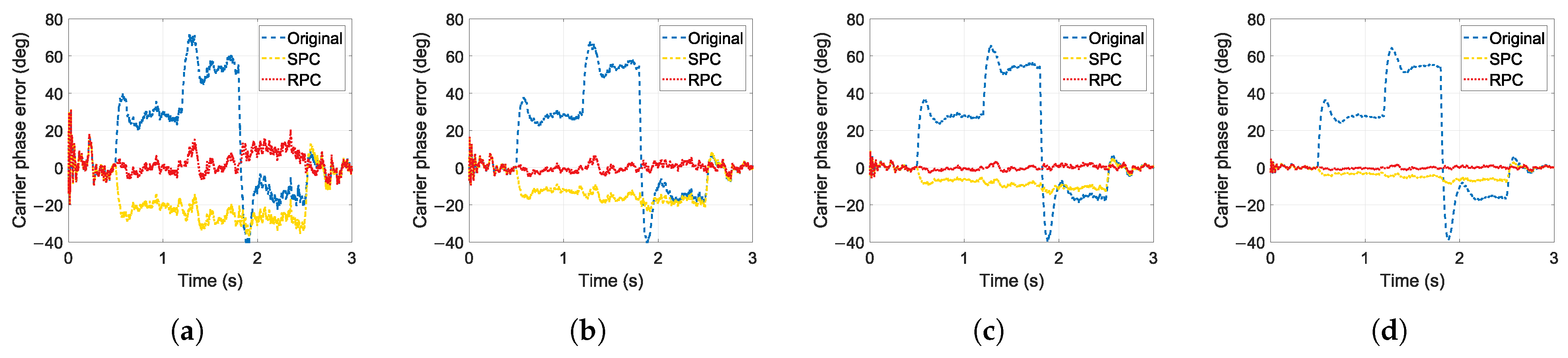
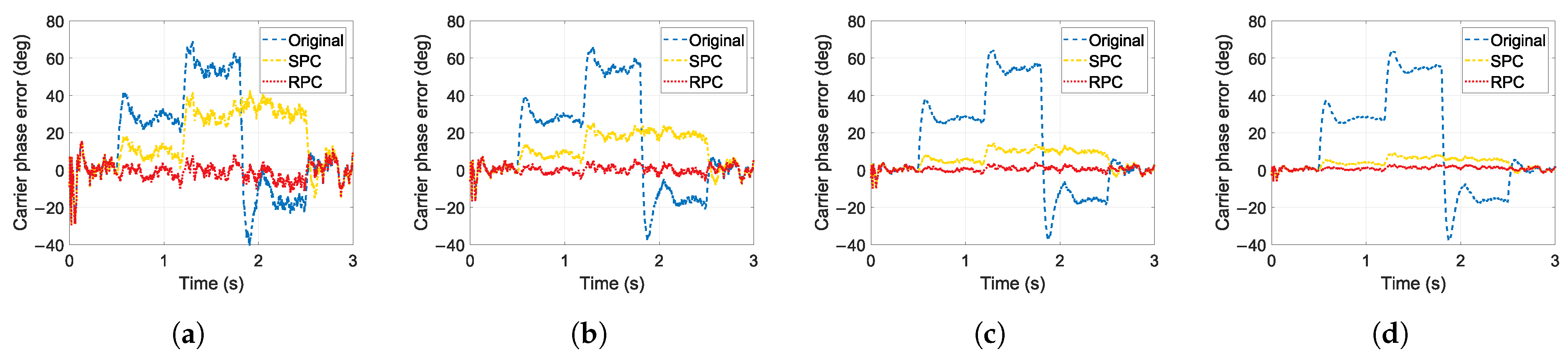
Figure 9 and Figure 10 show the carrier phase errors with and without phase compensation techniques at different $C/N_0$ conditions under Acc and Sin dynamics, respectively. The following results can be derived from these figures. (1) From the original curves at different $C/N_0$ conditions in the two figures, it can be seen that increasing $C/N_0$ does not reduce the amplitude of the phase bias because the GNSS is still buried under the noise floor and it has a tiny effect on the array weight. However, increasing $C/N_0$ can slightly reduce the amplitude of transient overshoots. (2) From the SPC and RPC curves at different $C/N_0$ conditions in the two figures, it can be seen that the residual phase bias after compensation in these two phase compensation techniques decreases as the $C/N_0$ increases. This suggests that a higher $C/N_0$ makes the phase bias estimation more accurate and thus improves the performance. This is consistent with the results in Section 4.1. (3) Comparing the SPC and RPC curves at the same $C/N_0$ conditions in the two figures, it is shown that the RPC has better phase compensation performance than the SPC, resulting in a significant improvement in measurement accuracy. This is because the RPC has better phase bias estimation than the SPC, as shown in Section 4.1. (4) The RPC shows the expected performance at different $C/N_0$ conditions under different dynamics. By using the RPC, the phase distortions are significantly reduced after phase bias estimation and compensation. This proves the applicability of the proposed technique.

Figure 9. Carrier phase errors with and without phase compensation techniques under Acc dynamics. (a) 35 dB-Hz. (b) 40 dB-Hz. (c) 45 dB-Hz. (d) 50 dB-Hz.

Figure 10. Carrier phase errors with and without phase compensation techniques under Sin dynamics. (a) 35 dB-Hz. (b) 40 dB-Hz. (c) 45 dB-Hz. (d) 50 dB-Hz.

5. Conclusions

In this paper, a robust phase compensation technique was proposed to maintain carrier phase measurement accuracy while suppressing interference using an antenna array. The main contributions of this work are summarized as follows:

(1)

The phase bias detection method was presented, which allows phase compensation techniques to be used in practice. It can locate the phase bias appearance time and trigger phase compensation techniques to start phase bias estimation and compensation.

(2)

The phase bias estimation method was studied and the robust estimation was applied to the phase bias estimation, making the proposed technique outperform existing phase compensation techniques in terms of accuracy and robustness.

There are still several limitations to this work, and the following future work is worthy of further investigation:

(1)

The window size in the proposed technique is fixed in this work; however, the selection of the window size requires more attention, and an adaptive window size may be more appropriate to balance the estimation accuracy and the dynamic performance.

(2)

The scale of the estimated phase bias is limited by the phase discriminator; if the phase bias is beyond the detection range of the discriminator, the phase bias cannot be accurately estimated. This issue should be addressed in future work.

References

- Gupta, I.J.; Weiss, I.M.; Morrison, A.W. Desired features of adaptive antenna arrays for GNSS receivers. Proc. IEEE 2016, 104, 1195–1206. [Google Scholar] [CrossRef] [Scilit]
- Craven, P.; Wong, R.; Fedora, N.; Crampton, P. Studying the effects of interference on GNSS signals. In Proceedings of the 2013 International Technical Meeting of the Institute of Navigation, San Diego, CA, USA, 27–29 January 2013; pp. 186–893. [Google Scholar]
- Compton, R. The power-inversion adaptive array: Concept and performance. IEEE Trans. Aerosp. Electron. Syst. 1979, 15, 803–814. [Google Scholar] [CrossRef] [Scilit]
- Huang, L.; Lu, Z.; Xiao, Z.; Ren, C.; Song, J.; Li, B. Suppression of jammer multipath in GNSS antenna array receiver. Remote Sens. 2022, 14, 350. [Google Scholar] [CrossRef] [Scilit]
- Arribas, J.; Fernandez-Prades, C.; Closas, P. Antenna array based GNSS signal acquisition for interference mitigation. IEEE Trans. Aerosp. Electron. Syst. 2013, 49, 223–243. [Google Scholar] [CrossRef] [Scilit]
- Church, C.M.; O’Brien, A.J.; Gupta, I.J. A novel method to measure array manifolds of GNSS adaptive antennas. Navigation 2011, 58, 345–356. [Google Scholar] [CrossRef] [Scilit]
- Chuang, Y.C.J.; Gupta, I.J. Antenna induced biases in GNSS receiver measurements. In Proceedings of the 2013 International Technical Meeting of The Institute of Navigation, San Diego, CA, USA, 27–29 January 2013; pp. 164–171. [Google Scholar]
- De Lorenzo, D.S.; Rife, J.; Enge, P.; Akos, D.M. Navigation accuracy and interference rejection for an adaptive GPS antenna array. In Proceedings of the 19th International Technical Meeting of the Satellite Division of The Institute of Navigation (ION GNSS 2006), Fort Worth, TX, USA, 26–29 September 2006; pp. 763–773. [Google Scholar]
- Yang, X.; Wang, F.; Liu, W.; Chen, F. A new blind anti-jamming algorithm based on a novel antenna array design. IET Radar Sonar Navig. 2022, 16, 1616–1626. [Google Scholar] [CrossRef] [Scilit]
- Daneshmand, S.; Marathe, T.; Lachapelle, G. Millimetre level accuracy GNSS positioning with the blind adaptive beamforming method in interference environments. Sensors 2016, 16, 1824. [Google Scholar] [CrossRef] [Scilit] [PubMed]
- Xu, H.; Cui, X.; Lu, M. Effects of power inversion spatial only adaptive array on GNSS receiver measurements. Tsinghua Sci. Technol. 2018, 23, 172–183. [Google Scholar] [CrossRef] [Scilit]
- Zhang, Y.D.; Amin, M.G. Anti-jamming GPS receiver with reduced phase distortions. IEEE Signal Process. Lett. 2012, 19, 635–638. [Google Scholar] [CrossRef] [Scilit]
- Jia, Q.; Wu, R.; Wang, W.; Lu, D.; Wang, L. Adaptive blind anti-jamming algorithm using acquisition information to reduce the carrier phase bias. GPS Solut. 2018, 22, 99. [Google Scholar] [CrossRef] [Scilit]
- OBrien, A.J.; Gupta, I.J. Mitigation of adaptive antenna induced bias errors in GNSS receivers. IEEE Trans. Aerosp. Electron. Syst. 2011, 47, 524–538. [Google Scholar] [CrossRef] [Scilit]
- Zhao, H.; Lian, B.; Feng, J. Adaptive beamforming and phase bias compensation for GNSS receiver. J. Syst. Eng. Electron. 2015, 26, 10–18. [Google Scholar] [CrossRef] [Scilit]
- Wu, J.; Tang, X.; Huang, L.; Ni, S.; Wang, F. Blind adaptive beamforming for a global navigation satellite system array receiver based on direction lock loop. Remote Sens. 2023, 15, 3387. [Google Scholar] [CrossRef] [Scilit]
- Xie, G. Principles of GPS and Receiver Design; Publishing House of Electronics Industry: Beijing, China, 2009. [Google Scholar]
- O’Driscoll, C.; Lachapelle, G. Comparison of traditional and Kalman filter based tracking architectures. In Proceedings of the European Navigation Conference, Napoli, Italy, 3–6 May 2009; pp. 3–6. [Google Scholar]
- Sun, Y.; Chen, F.; Lu, Z.; Wang, F. Anti-jamming method and implementation for GNSS receiver based on array antenna rotation. Remote Sens. 2022, 14, 4774. [Google Scholar] [CrossRef] [Scilit]
- Yang, Y.; He, H.; Xu, G. Adaptively robust filtering for kinematic geodetic positioning. J. Geod. 2001, 75, 109–116. [Google Scholar] [CrossRef] [Scilit]
- Yang, Y.; Xu, J. GNSS receiver autonomous integrity monitoring (RAIM) algorithm based on robust estimation. Geod. Geodyn. 2016, 7, 117–123. [Google Scholar] [CrossRef] [Scilit]
Disclaimer/Publisher’s Note: The statements, opinions and data contained in all publications are solely those of the individual author(s) and contributor(s) and not of MDPI and/or the editor(s). MDPI and/or the editor(s) disclaim responsibility for any injury to people or property resulting from any ideas, methods, instructions or products referred to in the content. |
© 2023 by the authors. Licensee MDPI, Basel, Switzerland. This article is an open access article distributed under the terms and conditions of the Creative Commons Attribution (CC BY) license (https://creativecommons.org/licenses/by/4.0/).