


Abstract
Enhancing traffic flow stability is a critical approach for achieving energy conservation and emission reduction in road transportation. While existing cooperative car-following strategies for connected and automated vehicles (CAVs) are effective, their heavy reliance on reliable Vehicle-to-Everything (V2X) communication limits practical deployment. This study proposes an energy-optimal car-following model for CAVs, introducing a regulation term based on the predicted optimal speed difference. Rather than directly using predicted kinematic variables, this mechanism adjusts acceleration based on the difference in optimal velocity between predicted and current headways. This leverages the inherent filtering of the optimal velocity function to ensure smooth control. Linear and nonlinear stability analysis confirm the model’s effectiveness in suppressing traffic disturbances and suppression of stop-and-go wave propagation, thereby laying the theoretical foundation for smoother traffic flow and the resulting reductions in energy consumption and emissions. Simulations validate the theoretical findings. Compared to the classical Full Velocity Difference (FVD) model, the proposed model achieves significant reductions in energy consumption (38.82%), CO2 emissions (39.41%), and NOx emissions (83.46%). The model also reduces rear-end collision risks, ensuring higher safety. These findings indicate that the proposed ego-vehicle predictive framework provides a communication-independent and practically viable approach for improving the energy efficiency and stability of CAV traffic flow.
1. Introduction
Global climate change and energy sustainability challenges have rendered energy conservation and emission reduction a central concern for governments and international organizations worldwide. The persistent growth of greenhouse gas emissions has intensified extreme weather events and environmental degradation, posing long-term risks to economic development and social stability. Air pollution such as PM2.5 and nitrogen oxides can adversely affect overall health [1], increase the risk of stroke [2], and lead to premature death [3], which has a negative impact on residents’ quality of life. In response, international frameworks such as the Paris Agreement and national carbon neutrality roadmaps have emphasized the necessity of reducing fossil energy consumption while improving system-level energy efficiency. A total of 195 countries have set a goal of achieving net-zero carbon emissions and limiting global warming to 1.5 °C by 2050 [4]. Within this context, suppressing unnecessary energy waste through technological and operational optimization has been widely recognized as one of the most cost-effective and scalable pathways to achieve emission reduction targets. Consequently, proposing mechanisms that can simultaneously enhance system stability and energy efficiency has become an urgent research priority.
Due to the rapid growth of road traffic demand and vehicle ownership, the transportation sector stands as a major contributor to global energy consumption and carbon emissions among all end-use sectors [5,6], presenting a critical challenge for climate mitigation goals. According to data from the IEA [7], total global CO2 emissions from fuel combustion reached 34,691.7 million tons in 2023. The road transport sector accounted for 6196.6 million tons, representing approximately 17.9% of total global CO2 emissions from fuel combustion. Accordingly, a wide range of strategies such as vehicle electrification [8,9], intelligent transportation systems [10,11], and traffic flow optimization [12,13,14] have been proposed to reduce transportation-related emissions. Compared with approaches relying solely on energy substitution, improving traffic operational efficiency presents a readily deployable strategy with universal applicability. It reduces energy losses inherent in congestion, delivering immediate fuel savings and emission reductions regardless of vehicle powertrain. This establishes traffic flow optimization as a pivotal and synergistic component of comprehensive transportation decarbonization efforts.
At the microscopic level, vehicle car-following behavior constitutes the fundamental unit of traffic flow. Transportation energy consumption and emissions originate from vehicle power output behaviors, which are intrinsically governed by longitudinal motion control and car-following dynamics. Empirical and theoretical studies have consistently demonstrated that traffic flow instability, which is characterized by frequent acceleration, deceleration, and stop-and-go oscillations, significantly increases vehicle energy consumption and pollutant emissions, especially under medium traffic densities [15,16]. Conversely, stable and smooth car-following behavior can effectively reduce power fluctuation amplitudes, leading to lower fuel consumption or electricity use and reduced emissions per unit distance traveled. Therefore, from a control-theoretic perspective, enhancing traffic flow stability through appropriate vehicle dynamics regulation constitutes a fundamental mechanism for achieving energy-efficient and low-emission traffic operations.
The emergence of connected and automated vehicles (CAVs) offers a revolutionary technological pathway to achieve the aforementioned vehicle dynamics regulation. Unlike traditional human-driven vehicles, which are constrained by driver reaction delays and limited perception, CAVs leverage Vehicle-to-Everything (V2X) communication to acquire and integrate real-time traffic state information beyond line-of-sight. This capability significantly improves precision and coordination in speed and headway control [17,18,19,20,21]. It marks a shift in the car-following paradigm from reactive response to proactive information utilization and collaborative planning. Numerous researchers have leveraged real-time platoon state information obtained through V2X to design multi-vehicle cooperative car-following models. By optimizing cooperative strategies among vehicles, these approaches systematically regulate vehicular dynamics, facilitate smoother car-following behavior, and thereby achieve reductions in energy consumption and emissions. Guo et al. [22] introduced the offset information of the current instantaneous speed relative to the recent historical speed mean based on the Full Velocity Difference (FVD) model, smoothing the vehicle acceleration curve and thereby reducing energy consumption and emissions. Kang et al. [23] proposed a discrete following controller based on the average optimal speed of the preceding two successive vehicles, which effectively improves the stability of traffic flow and significantly reduces energy consumption and CO2 emissions. Zhang et al. [24] proposed using V2X communication to obtain the average headway of multiple downstream vehicles as compensation information, reducing unnecessary fuel consumption and emissions. Wang et al. [25] incorporated weighted information on the speed and acceleration of multiple preceding vehicles building upon the traditional LCM model, thereby developing a Cooperative Look-ahead Car-following Model (CLCM) to achieve reduced energy consumption.
Existing research has confirmed the effectiveness of optimizing car-following behavior in energy conservation and emission reduction. In many scenarios, communication quality cannot be consistently guaranteed, such as when platoons travel through limited network coverage, environmental occlusion, or device-level constraints. These situations can cause significant communication delays or packet loss [26,27]. Such communication imperfections may influence the timeliness and completeness of shared information, which can in turn affect cooperative car-following performance. This may increase the likelihood of traffic conflicts and negatively affect traffic safety and efficiency [28,29].
In multi-vehicle cooperation, vehicles can use information from preceding vehicles to guide powertrain regulation, thereby smoothing speed fluctuations and reducing energy consumption and emissions. This benefit arises because the motion of the leading vehicle provides short-term anticipatory information for following vehicles. If a vehicle can instead predict its own near-future driving demands from its current state, anticipatory control can be achieved without relying on real-time observations of other vehicles. This idea forms the basis of communication-independent predictive control, and has motivated recent studies on ego-vehicle-based prediction. Wu et al. [30] designed a model that predicts the relative speed with the preceding vehicle at a future moment and adjusts its own acceleration based on the difference between this predicted value and the current relative speed. Yadav et al. [31] simultaneously introduced predictive information regarding the future headway and future speed of the preceding vehicle into the FVD model, demonstrating that the model can expand the stable region of traffic flow and suppress the formation of congestion. Pogrebnyak [32] proposed a traffic flow model that predicts the dynamics of the second vehicle ahead, thereby optimizing car-following behavior.
These studies confirm that models with predictive information can effectively enhance traffic flow stability and suppress congestion. A common thread among them is the direct utilization of predicted kinematic variables, such as future relative speed and headway, as immediate inputs to the car-following controller. Models that directly forecast future kinematic states and employ these predictions as immediate control targets face practical challenges in stability and smoothness, as any prediction error or transient fluctuation can be amplified into abrupt acceleration or deceleration commands. This amplification mechanism risks inducing significant vehicle jerk. This sensitivity necessitates additional filtering to ensure robust operation, which may limit performance across diverse driving scenarios.
To address this limitation while retaining the stability-enhancing potential of ego-based prediction, we develop an energy-optimal car-following model for CAVs that integrates headway forecasting into an optimal velocity difference framework. The optimal velocity function naturally smooths high-frequency variations in predicted headway and translates them into gradual acceleration responses. By expressing predictive correction in the form of velocity differences within the classical optimal velocity framework, the controller maintains the damping characteristics of established car-following models. In this way, predictive information is integrated as a complement to a stable feedback structure rather than as a direct control target. This design enables vehicles to adjust their longitudinal behavior in advance based on anticipated traffic evolution, shifting from purely reactive responses toward prediction-assisted regulation. This formulation also clarifies the distinction from existing predictive strategies: unlike look-ahead or multi-preceding-vehicle models that rely on upstream vehicle information via V2X, the proposed model is purely ego-based and requires no external data. Moreover, unlike delayed models that compensate for driver reactions using past information, the proposed model predicts future headway to enhance traffic flow stability, representing an anticipatory rather than compensatory mechanism.
The rest of this paper is structured as follows. Section 2 discusses the relationship between energy consumption, emissions, and vehicle longitudinal control. Section 3 introduces the proposed energy-optimal car-following model with headway forecasting and optimal velocity difference control. Section 4 presents theoretical stability analysis and numerical simulations to validate the model’s effectiveness. Section 5 evaluates the model’s performance in terms of energy consumption, emissions and safety. Section 6 concludes the paper with a summary of findings. Section 7 discusses the limitations of this study and suggests directions for future research.
2. Relationship Between Energy Consumption, Emission Reduction, and Vehicle Longitudinal Control
Energy consumption and pollutant emissions in transportation systems fundamentally originate from vehicle power output at the microscopic level, which is governed by longitudinal dynamics. Studies show that energy consumption responds nonlinearly to power demand, meaning frequent and large acceleration fluctuations significantly increase fuel use and exacerbate emissions. In traffic flow, such aggressive accelerations are often not voluntary but are forced by flow instability. Under moderate densities, small disturbances such as lane changes or sudden braking [33] can amplify into persistent stop-and-go waves, trapping vehicles in repeated acceleration-braking cycles far from their energy-optimal operating points. This mechanism is recognized as a major source of hidden energy waste and excess emissions in road transport systems [6,34,35].
Therefore, smoothing longitudinal dynamics by suppressing traffic oscillations is a direct pathway to reducing energy waste. The model proposed in the next section integrates headway forecasting and optimal-velocity-difference feedback to achieve this stabilization, thereby linking improved traffic flow stability directly to energy savings.
3. Energy-Optimal Car-Following Model with Headway Forecasting and Optimal Velocity Difference Control
To circumvent the reliability limitations of communication-dependent strategies, this chapter proposes an energy-optimal car-following model that incorporates headway prediction into the optimal speed difference control framework.
3.1. Baseline Car-Following Dynamics
Consider a single-lane traffic system consisting of identical vehicles indexed by . Let , , and denote the position, velocity, and acceleration of vehicle at time , respectively. The headway between vehicle and its preceding vehicle is defined as follows:
In classical car-following theory, automated controllers attempt to adjust their velocity toward an optimal velocity function , which represents the desired speed given the available headway. To enhance responsiveness to relative motion, the FVD model [36] further incorporates the velocity difference between consecutive vehicles. The general form of the baseline dynamics can be expressed as
where is the sensitivity coefficient, is the speed difference sensitivity coefficient, represents the speed difference between the th and th vehicles. Although this structure improves traffic flow stability compared with purely optimal velocity-based models, it remains reactive in nature and does not explicitly account for future traffic evolution or energy efficiency considerations.
3.2. Optimal Velocity Difference Control
In car-following behavior, the headway is the most direct state parameter determining driving safety and efficiency. To achieve forward-looking control and enhance energy efficiency, predicting the headway is crucial. However, directly using the predicted headway as the control target may lead to abrupt changes in acceleration commands, which is not conducive to generating a smooth trajectory. Therefore, this study proposes an innovative method centered on an “optimal speed difference”. This term is derived by mapping both the predicted and current headway to the optimal velocity function and calculating their difference, and is then embedded as the core adjustment term in the acceleration equation. The proposed model is formulated as:
where is the response coefficient associated with the predicted optimal velocity difference; represents the prediction intensity coefficient, weighting the forecasted headway change; indicates the prediction time, defining how far ahead the system forecasts traffic states. The future headway is approximated by the first-order kinematic relation . The additional term enables vehicles to adjust their acceleration in anticipation of future headway changes, thereby reducing unnecessary power fluctuations caused by delayed reactions. Unlike predictive control approaches that directly forecast vehicle speed or acceleration, the proposed formulation operates at the level of optimal velocity regulation, preserving the simplicity and interpretability of classical car-following models while embedding forward-looking information. The schematic of this control framework is illustrated in Figure 1.
Figure 1.
The connected and automated vehicle (CAV) car-following scenario utilizing predicted information.
The proposed control structure shifts the predictive objective from external observation to internal state extrapolation, diminishing the need for real-time preceding vehicle data and its associated communication vulnerabilities. More critically, instead of using the predicted headway directly as a spacing target, this model processes the prediction through the optimal velocity function. Because , the velocity difference term in the proposed model is inherently constrained within a reasonable range. This structural property prevents excessive control amplification and keeps the compensation term well bounded. Moreover, the mapping through the optimal velocity function acts as a natural low-pass filter, attenuating small fluctuations in headway prediction. In the following sections, linear stability analysis and nonlinear analysis based on the modified Korteweg-de Vries (mKdV) equation are conducted to rigorously investigate the impact of the predicted optimal velocity difference term on traffic flow stability and jam wave propagation. Numerical simulations are further performed to quantify the resulting improvements in energy consumption, emissions, and safety performance.
4. Stability Enhancement Through Predictive Control
Traffic flow oscillations are a primary cause of additional energy consumption. The fundamental prerequisite for a car-following model to achieve energy conservation and emission reduction lies in its ability to maintain stable traffic flow and suppress the generation and amplification of oscillations. Therefore, it is necessary to conduct a stability analysis on the model.
4.1. Linear Stability Analysis
This section will conduct a linear stability analysis of the model to verify its effectiveness in maintaining stable traffic flow, thus laying the foundation for analyzing energy conservation and emission reduction. Using the Laplace method, we analyze how the predicted headway and optimal velocity difference influence stability by treating disturbance propagation between consecutive vehicles as a system and transforming it from the time domain to the frequency domain.
First, assuming the traffic flow is in a steady state with all vehicles maintaining a constant headway , the linearization of Equations (3) and (4) leads to the following linear differential equation:
Applying the Laplace transform of Equation (5) and simplifying yields the expression in the frequency domain:
Thus, the transfer function is derived as:
For the system to be stable, the following condition must be satisfied:
Equation (8) ensures that any disturbance introduced into the platoon will attenuate as it propagates upstream from the th vehicle to the th vehicle. This attenuation characteristic is critical for preventing the amplification of speed fluctuations, which are the primary cause of stop-and-go waves and the associated increases in energy consumption and emissions.
When ,
The Taylor expansion of and are and . Thus, Equation (9) becomes
the coefficient of must be nonnegative, yielding the stability criterion:
Therefore, the condition of linear stability is
Equation (12) provides the critical stability criterion for the proposed model. It quantifies the minimum sensitivity required to prevent an infinitesimal speed fluctuation from amplifying into a growing traffic wave. A lower stability threshold permits the system to maintain stability even with reduced reaction sensitivity. The predictive parameters actively reduce the threshold by providing anticipatory compensation, thereby systematically expanding the stable operating region in parameter space and relaxing the design constraints on controller reactivity. Therefore, Equation (12) mathematically proves that the predictive mechanism injects an additional stabilizing force into the car-following dynamics. This lowered threshold is the theoretical basis for the model’s ability to maintain smoother traffic flow under a wider range of conditions. To visualize this relationship, we plotted a linear stability region diagram to illustrate the relationship between the sensitivity coefficient and the headway . Furthermore, by varying the prediction intensity coefficient , the response coefficient , and the prediction time , their respective influences on traffic flow stability were identified.
The linear stability curve divides the diagram into two distinct regions: the area above the curve represents the stable region, while the area below corresponds to the unstable region. The shape and position of this curve directly reflect the model’s ability to suppress traffic oscillations, which in turn influences vehicle energy consumption. As shown in Figure 2, the proposed prediction model exhibits clear differences in the linear stability diagram compared to the FVD model. Specifically, the curve of our model is lower than that of the FVD model, indicating a larger stable region. This improvement can be attributed to the predictive capability of the model.
Figure 2.
Stability region diagram in the plane.
Further analysis reveals that each predictive parameter systematically enlarges the stable region. In Figure 2a, increasing the prediction intensity coefficient lowers the stability curve, reflecting that stronger reliance on anticipated information improves disturbance rejection. Similarly, raising the response coefficient (Figure 2b) amplifies the corrective action from the predicted speed difference, further stabilizing flow. Extending the prediction time (Figure 2c) allows vehicles to accommodate future traffic variations earlier, promoting smoother, more gradual speed adjustments. Based on the above results, we can conclude that the introduction of the predicted optimal velocity difference in the model plays an effective role in maintaining traffic flow stability. This stability enhancement is essential for achieving smooth and efficient vehicle motion, thereby supporting the goal of energy conservation and emission reduction.
4.2. Derivation of Neutral and Coexistence Curves via Nonlinear Stability Analysis
The linear stability analysis presented in the previous subsection provides valuable insight into the conditions under which uniform traffic flow remains stable against small perturbations. However, linear analysis is inherently limited to infinitesimal disturbances and cannot fully capture the nonlinear evolution of traffic flow once perturbations grow beyond the linear regime. In real traffic systems, especially near the critical stability boundary, small disturbances may evolve into finite-amplitude congestion waves, leading to persistent stop-and-go patterns and substantial increases in energy consumption and emissions. To investigate the nonlinear characteristics of traffic flow near the onset of instability, it is necessary to analyze the system dynamics in the vicinity of the critical point identified by the linear stability condition. In this regime, weakly nonlinear effects become dominant and govern the formation, propagation, and saturation of congestion waves. A well-established approach for capturing such dynamics in car-following systems is the reductive perturbation method, which enables the derivation of evolution equations describing long-wavelength, small-amplitude traffic disturbances.
In the following, the reductive perturbation method is employed to derive Burgers and mKdV equations for the proposed energy-optimal car-following model. By analyzing these solutions, the influence of the predicted optimal velocity difference mechanism on the nonlinear stability properties, wave amplitude, and propagation behavior of congestion waves can be systematically examined. This analysis provides a deeper theoretical understanding of how predictive control enhances traffic flow stability and contributes to energy-efficient and low-emission traffic operations. For the purpose of facilitating nonlinear analysis, Equation (3) is reformulated as follows:
In this section, through perturbation analysis, we systematically investigate the dynamical behavior of the model near critical points, derive the Burgers and mKdV equations describing disturbance evolution, and obtain the neutral stability curve and the coexistence curve. By analyzing the influence of predictive parameters on the shape of these curves, we aim to analyze the mechanisms for suppressing traffic oscillations, thereby achieving smooth driving and providing a theoretical foundation for energy conservation and emission reduction.
4.2.1. Burgers Equation
When the traffic flow is linearly unstable, small speed fluctuations amplify and coalesce into sharp, propagating shock waves. The rate of decay and dissipation of this shock is directly linked to the system’s stability. To describe the formation and evolution of these shocks, we derive the Burgers equation from our car-following model. By examining how predictive parameters influence this dissipation, we assess their role in suppressing traffic oscillations and promoting energy-efficient driving.
We introduce the slow variables and as follows:
where is a constant to be determined, and is a small parameter characterizing the long-wavelength scale. The gap between adjacent vehicles can be expressed as:
Substituting Equations (14) and (15) into Equation (13) and then expanding to the third order of using Taylor expansion, the following partial differential equation is obtained:
where and .
To eliminate the secular terms that would lead to unbounded growth in the solution, we enforce the solvability condition at order be zero. This requires the coefficient of the resonant term to vanish, yielding . Substituting this value into Equation (16), we obtain:
The second-derivative term represents dissipative effects. A positive coefficient for this term indicates an inherent smoothing mechanism in the system, causing perturbations to decay over time. Therefore, when the coefficient of is greater than 0, it indicates that the traffic flow is stable; that is,
The derived results are consistent with the results of the linear stability analysis.
When >> 1, the triangular shock wave solution is described as Equation (19):
where is the precursor coordinate of the shock wave, and is the slope along the x-axis.
Equation (19) reveals how predictive control modifies shock wave dynamics. The tanh function describes a smooth transition between free flow and congested flow. The width of this transition zone in the denominator is modulated by the coefficient . A larger coefficient leads to a wider transition zone and faster dissipation of the shock. From Equation (19), it can be seen that the propagation speed of the triangular shock wave is determined by , and the shock wave propagates backward relative to the direction of vehicle motion. As the predictive parameters increases, the dissipation coefficient increases, causing the disturbance to decay to zero more rapidly. Consequently, the vehicle headway converges to the equilibrium headway . The attenuation of shock waves ensures that speed fluctuations from disturbances are damped effectively, preventing them from persisting as sustained stop-and-go oscillations. This smoothing effect directly reduces energy losses associated with braking energy dissipation and excessive fuel injection or power demand during sudden acceleration.
4.2.2. mKdV Equation
The mKdV equation is typically derived near the critical point () of linear stability analysis. At this point, the linear growth rate vanishes, rendering the linear analysis insufficient to capture the system’s dynamics. The mKdV equation describes the localized wave structures that emerge near the critical point, namely kink–antikink wave pairs, which correspond to moving congestion clusters in the coexistence phase. The propagation of these clusters creates substantial spatial and temporal speed fluctuations, leading to inefficient driving patterns associated with high energy consumption and emissions. Therefore, analyzing the solution of the mKdV equation and its amplitude is crucial for understanding the system’s behavior in the critical region and for optimizing control strategies to maintain a stable and energy-efficient traffic flow.
We analyze the system near the stability threshold by considering the marginally unstable regime. This is formalized by introducing a small parameter via:
This scaling implies that the system operates near the onset of linear instability, where the linear growth rate is vanishingly small, and nonlinear effects become dominant.
We introduce the slow variables and as follows:
Substituting this scaling along with the headway perturbation Equation (15) into Equation (13) and then expanding to the fifth order of using Taylor expansion, the following partial differential equation is obtained:
The coefficients are listed in Table 1.
Table 1.
Coefficient of .
To derive the standard mKdV equation free of lower-order perturbations, we systematically remove terms at orders and from Equation (22). The condition at order determines . This elimination procedure yields Equation (23).
The coefficients are listed in Table 2.
Table 2.
Coefficient of .
To cast Equation (23) into the canonical mKdV form that reveals universal nonlinear wave dynamics, we introduce the following regularization transformation:
Substituting Equation (24) into Equation (23) yields the regularized mKdV equation with a higher-order correction term:
where the perturbation term is given by
By disregarding , the kink–antikink wave solution of the mKdV equation is Equation (27):
The constant denotes the propagation speed of the congestion wave. To obtain the value of , the following solvability conditions need to be satisfied:
Evaluating this integral yields an explicit expression for :
Reverting to the original physical variables via the inverse of transformation of Equation (24), the kink–antikink soliton solution for the headway is obtained:
The amplitude of the kink–antikink wave solution is expressed as follows:
The kink–antikink soliton solution of the mKdV equation describes the coexistence phase. It mathematically describes a traveling transition wave that connects the free-flow and congested-flow phases. The amplitude of this soliton (as given by Equation (31)) quantifies the intensity of this transition. A larger signifies a steeper wave front, implying more abrupt changes in vehicle speed and headway. This translates to more severe and frequent acceleration/deceleration cycles, leading to higher energy consumption and emissions. The predictive mechanism introduced in our model can affect the growth of amplitude through its inherent regulation of nonlinear dynamics. This implies that, when the system is subjected to finite disturbances, predictive control can facilitate gentler and more gradual state transitions in traffic flow.
To intuitively illustrate the stability structure derived from the analyses, Figure 3 systematically characterizes the relationship between headway and sensitivity via two key boundaries derived from stability analysis. The neutral stability curve (solid) defines the onset of instability for uniform traffic flow, while the coexistence curve (dotted) results from nonlinear analysis, enclosing the parameter region where free and congested flows coexist as metastable states.
Figure 3.
Phase diagram in the plane (the solid line is neutral curve and the dash line coexistence curve).
Figure 3 illustrates how the neutral stability curves and the coexistence curves partition the parameter space into three distinct regimes: stable, metastable, and unstable. The region below the neutral stability curve corresponds to unstable traffic flow, where small perturbations are amplified and evolve into traffic oscillations. The region above the coexistence curve represents the stable regime, in which disturbances are fully dissipated and homogeneous flow is preserved. The intermediate region bounded by these two curves is identified as the metastable regime, where traffic flow remains linearly stable but may undergo nonlinear phase transitions under sufficiently large perturbations.
An increase in the prediction intensity coefficient indicates that vehicles make more effective use of anticipated headway information. Similarly, a larger response coefficient enhances the corrective influence of the predicted optimal velocity difference on vehicle acceleration, thereby accelerating the suppression of emerging disturbances. Extending the prediction time enables vehicles to incorporate traffic state variations further into the future, triggering earlier and more gradual speed adjustments. Through these mechanisms, vehicles can regulate their velocities in a smoother and more anticipatory manner, effectively preventing local perturbations from developing into nonlinear shock waves or inducing phase separation between free-flow and congested states.
As any of these parameters increase, both the neutral stability curve and the coexistence curve shift downward, resulting in a substantial expansion of the stable region. This geometric change carries direct physical implications. The descent of the neutral stability curve indicates that the model can effectively inhibit the cascading amplification of braking behaviors within the platoon, thereby preventing excessive dissipation of vehicle kinetic energy in the form of heat. The downward shift of the coexistence curve signifies an increase in the critical disturbance amplitude required to induce a persistent congestion cluster, improving the flow’s robustness to disturbances. Moreover, the lower coexistence curve corresponds to a reduction in the amplitude of the kink–antikink waves, implying a smaller velocity gap between free-flow and congested states. Consequently, transitions between traffic phases become smoother, leading to a reduction in peak kinetic energy dissipation and fuel consumption.
In summary, the expansion of the stable region illustrates that the predictive controller enhances the stability of traffic flow. It not only raises the threshold for congestion formation, but also mitigates the severity of congestion when it does occur. These attributes collectively form the dynamical foundation for reducing unnecessary acceleration work and fuel consumption.
4.3. Numerical Simulation
Although the linear stability analysis and nonlinear theoretical derivations provide valuable insights into the stability properties and wave dynamics of the proposed model, these analytical results are obtained under idealized assumptions. To further verify the theoretical predictions and to examine the model behavior under finite disturbances and realistic traffic scenarios, numerical simulations are indispensable. Specifically, the simulations aim to demonstrate how the introduction of the predicted optimal velocity difference influences traffic flow evolution and disturbance propagation under different parameter settings.
A numerical simulation environment was established to evaluate the proposed model. The setup consisted of a single-lane ring road with a length of 1200 m under periodic boundary conditions. A total of 100 vehicles were uniformly distributed along the road, each maintaining a target headway of 12 m and a target speed of 7.15 m/s. A small disturbance is introduced at the position of the 50th vehicle, defined as follows:
The disturbance is applied to the 50th vehicle as a representative choice; under periodic boundary conditions, applying the same disturbance to other vehicles yields qualitatively identical results. The total simulation duration is 1200 s, with a time step of 0.01 s. In this simulation scenario, the traffic flow disturbance propagates among all vehicles, enabling a comprehensive analysis of its impact on the entire platoon. Key control parameters were set as follows: sensitivity coefficient = 1.2, self-stabilizing information gain coefficient = 0.2. The optimal velocity function is defined as:
To investigate the influence of the prediction intensity coefficient on traffic dynamics, simulations were conducted under a fixed prediction time and response coefficient . Figure 4 depicts the dynamical evolution of headway between = 1000 s and 1200 s, illustrating the backward propagation of density waves over time.
Figure 4.
Headway evolution across the vehicles over time with fixed .
As shown in Figure 4, when a small disturbance is introduced into the traffic flow, kink–antikink waves emerge, and the headway oscillates within the range of approximately 6 m to 18 m. As the prediction intensity coefficient increases from 0 to 0.5, the amplitude of headway fluctuations gradually decreases and becomes confined to a narrower interval around 11.85–12.15 m. When is sufficiently large (), the oscillations are completely suppressed, and the headway converges to the desired equilibrium value of . With increasing , the overall stability of the system is significantly enhanced, as reflected by the progressive attenuation of spacing oscillations and the eventual disappearance of congestion waves. These results provide strong numerical validation for the theoretical analysis, confirming that the prediction intensity coefficient plays a crucial role in suppressing traffic flow fluctuations, smoothing vehicle speed variations, and reducing frequent acceleration and abrupt braking behaviors, thereby improving overall traffic stability.
Figure 5 illustrates the evolution of headway under a fixed prediction time and prediction intensity coefficient , while varying the response coefficient . As shown in Figure 5 when a disturbance is introduced, the traffic flow initially exhibits pronounced stop-and-go congestion. As the response coefficient increases, vehicles increasingly utilize predicted future-state information to generate compensatory control actions, leading to a gradual attenuation of traffic flow oscillations. When reaches an appropriate value (), the space headway distribution converges to a uniform profile, and the system transitions into a homogeneous flow state. An increase in effectively amplifies the contribution weight of the predicted information in the control law, enabling vehicles to generate smoother and earlier speed compensation commands. As a result, the operation of both the accelerator and braking systems becomes more gradual, significantly enhancing the disturbance rejection capability and self-stabilizing properties of the traffic system. This behavior provides a critical foundation for eco-driving by reducing unnecessary acceleration and deceleration cycles.
Figure 5.
Headway evolution across the vehicles over time with fixed .
Similarly, by fixing the prediction intensity coefficient at and the response coefficient at , the influence of the prediction time on traffic dynamics is further investigated. The corresponding simulation results are illustrated in Figure 6.
Figure 6.
Headway evolution across the vehicles over time with fixed .
The results presented in Figure 6 clearly illustrate the regulatory effect of the prediction time on traffic flow stability. When , the headway exhibits the largest fluctuation amplitude, and these oscillations persist without attenuation over time, indicating an unstable traffic state. As increases, the magnitude of headway fluctuations progressively decreases, reflecting a continuous enhancement in system stability. When reaches 0.5, the headway remains nearly constant throughout the entire simulation period, and the traffic flow converges to a homogeneous equilibrium state, confirming that the system has entered a stable regime. These findings demonstrate that the prediction time is a critical parameter for improving traffic flow stability. By extending the prediction horizon, vehicles are able to anticipate potential disturbances earlier and respond in advance, resulting in smoother and more gradual speed adjustments. Consequently, incipient disturbances are effectively dissipated before evolving into pronounced stop-and-go waves. This preemptive regulation mechanism avoids the high-energy-cost acceleration and braking cycles associated with congestion, thereby contributing to improved energy efficiency and reduced emissions.
Throughout the simulations, headway fluctuations remain strictly within safe limits, and no collisions are observed, demonstrating the strong robustness of the proposed model with respect to parameter variations. Notably, even under high prediction intensity, the system does not exhibit instability, indicating substantial safety margins for parameter calibration in practical implementations. Moreover, owing to the bounded nature of the optimal velocity function, , the velocity difference term in the proposed model is inherently constrained within a reasonable range. This structural property prevents unbounded amplification of control actions and ensures that the compensation term remains safe and well-regulated under all operating conditions.
4.4. Predictive Parameter Sensitivity Analysis
The simulations in Section 4.3 confirm the efficacy of the proposed predictive model in suppressing traffic oscillations and stabilizing flow under a nominal parameter set. To assess its practical applicability, the robustness of this stabilizing effect is further examined as the predictive parameters vary from their nominal values. This analysis focuses on determining whether excessively high gains lead to performance trade-offs and explores the limits of the model under extreme parameter combinations.
We conducted a sensitivity study that pushes individual predictive parameter to extreme levels, and further examines the compounded effects when multiple parameters are concurrently over-amplified. The macroscopic impact is quantified using traffic throughput, calculated as the product of space-mean speed and density.
Here, denotes the average speed of the vehicle platoon, and is the spatial density, where is the number of vehicles and is the road length. Throughput measures the number of vehicles passing a point per unit time and serves as an indicator of roadway capacity, providing insight into whether predictive control unintentionally reduces traffic efficiency.
To obtain a stable estimate, we computed over the fully developed flow period from to and derived the corresponding throughput under the same numerical simulation environment established in Section 4.3. For clearer interpretation, the resulting values are presented in vehicles per hour (veh/h). The results of this analysis are summarized in Table 3.
Table 3.
Traffic throughput under different levels of predictive parameter.
As summarized in Table 3, the traffic throughput remains virtually unchanged when any single predictive parameter is substantially increased, maintaining a level consistent with the proposed parameter set. This robustness persists even when two parameters are elevated to extreme values, with throughput showing no appreciable degradation. However, a performance trade-off occurs when all three parameters are simultaneously set to excessively high values, resulting in a measurable decline in throughput. This decline is linked to the dynamical behavior shown in Figure 7, which shows that under the condition which all parameters are extremely high, the velocity profile develops oscillations. These oscillations indicate an overcompensated and poorly damped response, which reduces the space-mean speed of the platoon, thereby directly accounting for the observed throughput decline.
Figure 7.
Comparison of instantaneous velocity at .
The sensitivity analysis indicates that the proposed predictive model maintains stability across a wide range of parameter variations. Specifically, traffic throughput is maintained when individual control gains are substantially increased, and it remains unchanged even when two parameters are simultaneously elevated. A decline in throughput only emerges when all three parameters are driven to extreme values, suggesting that the controller has a reasonable stability margin against perturbations in one or two parameters.
In summary, the numerical simulation results demonstrate that the proposed prediction mechanism effectively suppresses the propagation and amplification of traffic disturbances, thereby validating the theoretical advantages of the model in improving traffic flow stability and smoothness. These results not only provide strong numerical support for the analytical findings but also establish a solid empirical and theoretical foundation for the subsequent quantitative evaluation of traffic flow energy consumption and emission performance.
5. Results and Discussion
5.1. Analysis of Energy Consumption and Transportation Emissions
The theoretical and simulation analyses demonstrate that the prediction mechanism effectively enhances traffic flow stability through feedforward control. To quantify the energy-saving and emission-reduction benefits of the proposed predictive framework, this section employs the VT-Micro model [37] to assess the reduction rates in fuel consumption, CO2, and NOx emissions for the vehicle platoon. The performance is benchmarked against the classical FVD model, providing a direct validation of the model’s practical efficacy for sustainable transportation.
5.1.1. The VT-Micro Model
In this study, the VT-Micro model is adopted to estimate instantaneous fuel consumption and emissions based on vehicle kinematic states. The foundation of the VT-Micro model is an exponential function that relates the instantaneous fuel consumption or emission to the vehicle’s instantaneous speed and acceleration/deceleration. The basic formula is expressed as Equation (35):
where represents the measured output, which can be the fuel consumption rate (L/s) or the emission rate of pollutants (g/s); denotes the instantaneous vehicle speed (m/s); indicates the instantaneous vehicle acceleration (m/s2); and represents the model coefficients. This study employs the coefficient sets from He [38] and Li [15], which were derived from a recalibration of the model’s quadratic polynomial function to enhance its fidelity to real vehicle emission data. The parameters and listed in Table 4, Table 5 and Table 6.
Table 4.
Coefficients for the MOE of energy consumption.
Table 5.
Coefficients for the MOE of CO2 emission.
Table 6.
Coefficients for the MOE of NOx emission.
It should be noted that while the VT-Micro model has been widely validated for estimating emissions from conventional internal combustion engine vehicles, it has inherent limitations. The model’s coefficients are primarily calibrated using data from gasoline or diesel powertrains, meaning that the estimated values for energy consumption and emissions in electric or hybrid vehicles may require recalibration with specific data. Moreover, as a kinematics-based model, VT-Micro simplifies the complex transient responses of engines and after-treatment systems into polynomial functions of instantaneous speed and acceleration. While this simplification may impact the absolute magnitude of the estimated emissions, the model is generally accepted as robust for comparing the relative performance of different driving strategies under consistent simulation conditions, which is the primary objective of this study. Therefore, the reported reduction rates should be interpreted as indicative of the potential improvement enabled by the proposed predictive control framework, rather than as precise estimates for any specific vehicle type.
5.1.2. Results of Energy and Emission Reductions
The reductions in energy consumption and emissions reported in this subsection stem directly from the suppression of headway oscillations validated in Section 4. As evidenced by the transition from disordered to homogeneous headway distributions, the proposed predictive model stabilizes the platoon. This stabilization of headway facilitates eco-driving by dampening the amplitude and frequency of headway oscillations, which in turn suppresses high-order speed and acceleration terms in vehicle kinematics. Consequently, the kinematic inputs to the VT-Micro model are optimized, resulting in lower estimates of fuel consumption and pollutant emissions. Thus, the quantitative benefits presented below in this section are the direct metric outcome of the flow stabilization, which was validated in the preceding section.
Under the same numerical simulation environment established in Section 4.3, the VT-Micro model is used to estimate the energy consumption and transportation emissions of the vehicle platoon during the time period = 1000 s to 1200 s. To highlight the benefit of the predictive mechanism, we use the FVD model as the baseline, representing a purely reactive car-following strategy without predictive capability. This choice allows for a direct assessment of the incremental benefits conferred by the predictive mechanism, thereby serving to support the efficacy of the proposed forward-looking control architecture in enhancing energy-saving and emission-reduction performance. The energy saving/emission reduction rate is calculated as:
Figure 8a–c quantitatively delineate the influence of the key predictive parameters, namely, the prediction intensity coefficient , response coefficient , and prediction time , on the model’s energy-saving and emission-reduction performance. A consistent macroscopic trend is observed across all three parameters: the reduction rates for energy consumption, CO2, and NOx exhibit a rapid increase with rising parameter values. Notably, even modest predictive capability can still lead to substantial benefits, which indicates that the transition from no prediction to the introduction of a prediction mechanism is a critical phase for improving energy efficiency. After reaching a certain critical parameter value, the reduction rates tend to saturate and eventually reach a high-performance plateau with a 38.82% reduction in energy consumption, a 39.41% reduction in CO2 emission, and an 83.46% reduction in NOx compared to the FVD model. This demonstrates the effectiveness of incorporating prediction time in reducing energy consumption and traffic emissions. It also defines a practical operating range, within which the predictive controller delivers near-optimal efficiency while maintaining robustness.
Figure 8.
Reduction rates of energy consumption, CO2, and NOx emissions compared to Full Velocity Difference (FVD) model.
While a consistent macroscopic trend that performance improves before reaching saturation is observed for all three parameters, their distinct roles within the control architecture carry distinct implications for system design. The prediction intensity coefficient governs the trust placed on anticipated information. Figure 8a reveals that even a small (e.g., ) yields significant benefits, confirming that the mere shift from reactive to predictive operation is the primary enabler of efficiency gains. This underscores the fundamental value of feedforward control in preemptively damping disturbances that trigger wasteful acceleration fluctuations. The response coefficient acts as a gain on this predictive compensation. Figure 8b shows that as increases, energy-saving and emission-reduction benefits improve synchronously. As further increases, the growth rate of decline gradually slows down and eventually saturates as the traffic flow reaches a stable state. Therefore, a saturated platform can be seen as a working range that maintains performance improvement and robustness. Excellent and stable performance can be achieved when the is in the saturation region. The prediction time sets the temporal depth of the forward look. Figure 8c demonstrates that extending allows earlier and smoother interventions, avoiding late, sharp maneuvers. The saturation point of marks the boundary of the effective decision-making horizon for predictive information under the current system dynamics and information quality. This suggests that in practical system design, efforts should focus on improving the accuracy of predictions within the effective horizon, rather than blindly pursuing longer prediction sequences.
As shown in Figure 8, while the reduction rates of energy consumption and CO2 emissions are similar, NOx emissions decrease more significantly. This divergence arises from their distinct formation mechanisms. The following analysis links our model’s macroscopic emission outcomes to the microscopic vehicle dynamics it governs.
For internal combustion engines, instantaneous fuel consumption is primarily determined by the power demand required to overcome road load and provide acceleration. CO2 emissions are directly proportional to fuel consumption. Speed fluctuations influence the average road-load demand, whereas acceleration fluctuations generate transient power spikes that increase fuel use. NOx formation is strongly temperature-dependent and increases rapidly under high-load, high-temperature conditions. Hard acceleration typically raises in-cylinder temperature and pressure, creating favorable conditions for thermal NOx formation. As a result, NOx emissions respond in a highly nonlinear manner to aggressive acceleration.
To illustrate the microscopic kinematic smoothing effect of the predictive control, we present representative snapshot plots in Figure 9 and Figure 10, capturing the instantaneous velocity fluctuation and acceleration across the platoon at as a function of the prediction time . The influence of the prediction intensity coefficient and response coefficient on the kinematic states exhibits a highly similar qualitative trend, and is therefore omitted for conciseness.
Figure 9.
Snapshot of instantaneous velocity across vehicles under different prediction time at .
Figure 10.
Snapshot of instantaneous acceleration across vehicles under different prediction time at .
In Figure 9a, the FVD model exhibits stop-and-go waves, with speed fluctuating between approximately 2 and 12 m/s. Incorporating the predictive mechanism significantly attenuates these oscillations. With the introduction of the predictive parameter (Figure 9b), the speed range is progressively narrowed to 6.95–7.35 m/s. For sufficiently large , the oscillations become negligible, indicating traffic flow stabilization. This smoothing of the speed profile directly reduces the average tractive power demand, resulting in about 39% reductions in both energy consumption and CO2 emissions. The effect on acceleration is even more dramatic. The reactive FVD model generates sharp, high-magnitude acceleration/deceleration cycles in Figure 10a, ranging from −2.56 to 2.62 m/s2. The introduction of the prediction time τ fundamentally alters this dynamic, transforming the acceleration profile from a series of abrupt pulses into a smooth, continuous fluctuation. As shown in Figure 10c, the proposed predictive model compresses the acceleration range to approximately m/s2. This drastic reduction in acceleration amplitude is the key to understanding the disproportionate decline in NOx emissions. The underlying cause is the distinct formation mechanisms of the pollutants. CO2 emissions are stoichiometrically linked to fuel consumption, which responds proportionally to the reduction in overall kinematic variability achieved through speed smoothing. NOx formation is governed by high-temperature combustion, highly sensitive to extreme acceleration transients. By nearly eliminating these high-magnitude acceleration events, the predictive model directly suppresses the primary condition for thermal NOx generation. Therefore, while speed smoothing yields a proportional reduction in CO2, the targeted and severe suppression of acceleration extremes results in a disproportionately larger reduction in NOx emissions, explaining the observed disparity in reduction rates.
In summary, the parameters , , and collectively enable a transition from reactive to anticipatory control, with each parameter fine-tuning a specific aspect of the predictive action. The model achieves proportional reductions in energy and CO2 through fuel-efficient speed smoothing, while delivering disproportionately greater NOx abatement by suppressing the high-temperature combustion transients characteristic of aggressive acceleration and deceleration. These results underscore that the proposed predictive model not only conserves fuel but also actively mitigates traffic-related pollutant, offering a strategy for both carbon and air quality management in future transportation systems.
5.1.3. Robustness to Headway Prediction Errors
While the above results demonstrate significant energy and emission benefits under ideal prediction conditions, practical implementations inevitably involve prediction uncertainty. Therefore, evaluating the robustness of the proposed model under imperfect predictions is crucial. This section investigates the model’s sensitivity to prediction errors through simulation experiments, examining its stability and efficacy under noisy forecasts.
The prediction error is modeled as zero-mean Gaussian noise added to the predicted headway. The noise magnitude is defined as a percentage of the equilibrium headway ,
where represents the noise level coefficient. This formulation reflects relative prediction errors proportional to the following distance, which is consistent with practical sensing and estimation characteristics in car-following scenarios. Three representative noise levels are considered, including a low level of corresponding to high-accuracy perception, a moderate level of reflecting typical estimation uncertainty, and a high level of representing challenging perception conditions. All simulations are conducted under the stable parameter set (, , ) and compared with the noise-free baseline. Table 7 summarizes the performance metrics under different prediction noise levels.
Table 7.
Robustness analysis of model performance to headway prediction errors.
As the noise level increases, the energy-saving and emission-reduction benefits gradually decline, consistent with the expectation that prediction uncertainty weakens the effectiveness of anticipatory control. However, the performance degradation remains moderate. At a noise level of 2.5%, the reductions in energy consumption and emissions are nearly unchanged compared to the noise-free case, indicating that the model is insensitive to small prediction errors. At the level of 5%, performance remains around 90% of the ideal value, and the model continues to deliver most of its intended benefits. Even at a higher noise level of 10%, the model still achieves reductions of 29.25% in energy consumption, 30.50% in CO2 emissions, and 59.08% in NOx emissions relative to the FVD model.
These results demonstrate that the proposed strategy does not rely on highly accurate predictions and maintains substantial benefits under realistic prediction uncertainties. This robustness can be attributed to the smoothing and damping characteristics of the optimal velocity function, which mitigate the amplification of prediction noise.
5.1.4. Comparison with Energy-Efficient Car-Following Models
To further position the proposed model within the context of recent developments in car-following control, comparisons were conducted with two representative models proposed by Guo et al. [22] and Zhang et al. [24]. These models were selected because they explicitly incorporate traffic information from multiple preceding vehicles to improve fuel efficiency and reduce emissions, making them relevant benchmarks for assessing energy-environmental performance.
All models were implemented under the same simulation settings and evaluation framework. The parameter values of the comparison models were adopted from their original studies according to the recommended settings to ensure representative performance. The reduction rates of energy consumption, CO2, and NOx were calculated relative to the classical FVD model, enabling a direct comparison of the effectiveness of different control strategies. The values of for the Guo et al. and Zhang et al. models are adopted from their respective original studies to ensure consistency with their intended modeling frameworks. For the Guo et al. model, to avoid excessive table length while maintaining representativeness, only three typical cases () are reported, corresponding to low, medium, and high information availability levels. The comparative results are summarized in Table 8.
Table 8.
Comparison of relative energy and emission reductions with respect to the FVD model.
The comparative results indicate that the proposed model consistently achieves higher energy and emission reduction rates than the Guo et al. model across all tested values of . The advantage is particularly evident when only one preceding vehicle is considered. As the number of accessible preceding vehicles increases, the performance gap gradually narrows, which is expected since additional upstream information generally benefits multi-vehicle models. Nevertheless, the proposed model still maintains slightly superior reduction performance. Compared with the Zhang et al. model, the proposed model shows noticeably better performance when . When , the two models yield comparable reduction rates. This suggests that the predictive regulation based on headway forecasting can effectively translate limited information into smooth driving adjustments, achieving energy-saving effects similar to those obtained by exploiting downstream vehicle information.
Overall, these findings indicate that the proposed model achieves competitive or superior performance compared with recent energy-oriented car-following models. Notably, these benefits are obtained without requiring additional information from multiple preceding vehicles. The results therefore demonstrate that the proposed approach can deliver substantial energy and emission improvements while maintaining a relatively simple and communication-independent structure.
5.2. Analysis of Safety
The safety benefits reported in this study are inferred from the fundamental stabilization of traffic flow and the consequent elimination of collision events within our simulation framework, rather than being derived from formal probabilistic crash modeling. The core premise is that rear-end collisions in car-following scenarios are primarily caused by excessive speed differences and inadequate headway, both of which are intrinsically linked to traffic oscillations. The predictive model is designed to suppress oscillations and promote smoother car-following dynamics in simulation. The following analysis using Time-to-Collision (TTC) metrics provides quantitative surrogate measures to corroborate this inferred safety improvement by showing drastic reductions in both the duration and severity of near-crash situations. The formula for calculating TTC is given as Equation (38).
This metric calculates the time remaining until a collision occurs if two vehicles continue traveling at their current relative speed. A smaller TTC value indicates a higher risk of collision between the leading and following vehicles.
While instantaneous TTC is a direct measure of imminent danger, it fails to capture the temporal persistence or cumulative severity of risk exposure. Therefore, we adopt the Time Exposed Time-to-Collision (TET) and Time Integrated Time-to-Collision (TIT) metrics, which aggregate risk over time and space, offering a more robust evaluation of the model’s safety performance. The TET metric measures the total duration during the entire simulation in which the TTC value falls below a specified safety threshold (denoted as TTC*). This metric accounts for the persistence of risk and quantifies the total time the system remains in a hazardous state. A larger TET value indicates that vehicles are exposed to collision risk for a longer period. Here, t0 denotes the simulation time step.
The TIT metric calculates the integral of the TTC curve over the entire simulation period whenever the TTC value falls below the safety threshold. This indicator accumulates both the urgency and duration of collision risk, measuring the total magnitude of collision risk exposure. A higher TIT value indicates that vehicles frequently operate in hazardous conditions with elevated collision risk.
The safety contribution of the predictive mechanism is quantified using the same simulation environment and parameter settings established in Section 4.3. TTC-based metrics are adopted to evaluate safety performance. Simulation data indicate that TTC values in the studied scenario are above 2.0 s, with the baseline FVD model’s minimum TTC at 2.26 s. Therefore, thresholds of 3.0 s and 4.0 s are adopted to quantify safety margins within the observed TTC range, enabling meaningful comparison of safety performance against the baseline FVD model.
The proposed model is systematically compared to the baseline FVD model by computing the relative reduction in TET and TIT metrics. The percentage reductions achieved are illustrated in Table 9 and Table 10, where the prediction intensity coefficient is varied, and the response coefficient and prediction time fixed at , respectively.
Table 9.
Reduction percentage of Time Exposed Time-to-Collision (TET) compared to FVD model under different .
Table 10.
Reduction percentage of Time Integrated Time-to-Collision (TIT) compared to FVD model under different .
When the safety threshold is set to TTC* = 3.0 s, both the TET and TIT reduction rates increase with . When reaches a sufficiently high value (, these reduction rates achieve 100%. This indicates that within the scope of our simulation setup of a homogeneous platoon on a ring road with a single initial disturbance, the predictive controller is capable of completely suppressing the conditions that lead to TTC values below the chosen safety thresholds. These results represent the upper bound of safety performance achievable by the model under idealized conditions, demonstrating its strong potential for collision risk mitigation. Under a more relaxed threshold of TTC* = 4.0 s, even a modest yields substantial reduction rates, indicating that limited predictive capability is already highly effective in suppressing moderate-risk conditions, reflecting the model’s inherent robustness in common driving situations.
Table 11 and Table 12 present the reduction rates of TET and TIT under different response coefficient values, while the other predictive parameters are held constant (, ).
Table 11.
Reduction percentage of TET compared to FVD model under different .
Table 12.
Reduction percentage of TIT compared to FVD model under different .
Under the TTC* = 3.0 s criterion, increasing increases TET and TIT reduction rate until complete risk elimination is achieved at , indicating that amplifying the predictive compensation term enables the controller to fully resolve imminent hazards. Under the safety threshold of TTC* = 4.0 s, the advantage of the proposed model becomes even more pronounced. Even with a small , the system eliminates nearly 99% of moderate-risk situations, demonstrating that even modest predictive weighting is sufficient to mitigate the majority of moderate-risk scenarios, reflecting the model’s inherent robustness in common driving environments.
Table 13 and Table 14 present that the prediction time exhibits a safety improvement trend similar to that of the response coefficient . Under the strict TTC* = 3.0 s criterion, the reduction rates of both TET and TIT increase with , achieving 100% reduction at . This consistency confirms that lengthening the forward-looking window also systematically enhances collision avoidance.
Table 13.
Reduction percentage of TET compared to FVD model under different .
Table 14.
Reduction percentage of TIT compared to FVD model under different .
The proposed optimal speed difference prediction model effectively reduces both TIT and TET metrics. It attains a 100% reduction rate in TET and TIT, suggesting that collision risk is virtually eliminated within the scope of the simulation once key parameters exceed their critical values. These results demonstrate that the control strategy substantially enhances proactive safety in car-following by more effectively suppressing rear-end collision risks, thereby offering a reliable control framework for safety assurance in connected and automated vehicles.
The environmental and safety benefits quantified in Section 5.1 and Section 5.2 are derived from simulations of a homogeneous CAV platoon under a single-lane ring-road scenario with a single initial disturbance. It should be acknowledged that the absolute reduction rates are therefore scenario-specific. These rates may vary under heterogeneous traffic, open-boundary conditions, or different disturbance patterns. Moreover, in real-world deployments, factors such as prediction inaccuracies would inevitably introduce disturbances that are not accounted for in this study. While these practical factors may reduce the absolute reduction rates, the model’s core mechanism of anticipatory longitudinal smoothing remains fundamentally robust. Therefore, the proposed strategy is expected to deliver significant improvements compared to conventional reactive models, providing a reliable foundation for developing more sustainable and safer next-generation driving systems.
5.3. Theoretical Performance Analysis Across Traffic Densities
The energy and emission benefits demonstrated in this work are intrinsically linked to the suppression of stop-and-go oscillations, which are most prevalent under moderate traffic densities where the flow is metastable. It is important to contextualize these findings within the broader framework of traffic flow theory. Accordingly, we analyze the model’s performance across different traffic densities, focusing on low-density and high-density regimes.
In low density conditions, the traffic stream operates in a free-flow state, with minimal inter-vehicle interactions and inherent stability. Consequently, the energy-saving potential of any oscillation-damping strategy, including our predictive model, is relatively small. However, the model’s ability to generate smooth acceleration profiles still contributes to marginal fuel savings and reduces high-transient NOx emissions during occasional car-following events. In contrast, under heavy congestion and near-capacity conditions, the average spacing between vehicles approaches the minimum safety distance, severely constraining the kinematic freedom of longitudinal motion. In this state, there is little room for effective eco-driving maneuvers without compromising safety. Consequently, the potential for fuel savings through speed smoothing is inherently constrained by the congested conditions. However, the predictive model remains valuable by controlling transient dynamics within the constrained flow. It can modulate the timing and gradient of deceleration waves, preventing them from steepening into sudden braking events that are both hazardous and energy-intensive. In congested conditions, the predictive model enhances safety by reducing collision risks and mitigating the energy consumption and exhaust emissions arising from abrupt acceleration and deceleration events.
In summary, the efficacy of the predictive model is density-dependent. Its energy-saving potential is highest in the moderate-density regime, where suppressing stop-and-go oscillations offers the maximum benefit. In free-flow conditions, the model primarily reduces transient emissions, while in congested conditions, the focus shifts to safety and the prevention of energy-wasting power transients. These theoretical insights provide context for the significant reductions reported in this study and clarify the operational conditions where the proposed strategy has the most significant impact.
6. Conclusions
Motivated by the urgent need for traffic-related energy conservation and emission reduction, this study proposes an energy-optimal car-following model. Its core is a predictive regulation mechanism that forecasts headway and utilizes the resulting optimal velocity difference to adjust acceleration. This enables smoother vehicle motion, directly targeting the suppression of energy-wasting stop-and-go waves.
Through linear stability analysis, the critical stability conditions of the proposed model were analytically derived. The results demonstrate that the inclusion of the predicted optimal velocity difference significantly enlarges the stable region in the parameter space compared with the classical FVD model. We systematically examined the effects of key predictive parameters, including the prediction intensity coefficient , response coefficient , and prediction time . The results reveal that stronger predictive capability and longer anticipation horizons effectively suppress traffic oscillations and enhance flow stability, even under relatively low sensitivity conditions. Furthermore, nonlinear analysis based on the reductive perturbation method was conducted near the critical point. By deriving the Burgers equation and the mKdV equation, the evolution characteristics of small disturbances and jam waves were analytically characterized. The results indicate that the proposed predictive mechanism not only accelerates the attenuation of shock waves in the stable region but also reduces the amplitude of kink–antikink waves in the metastable regime. This leads to smoother transitions between free-flow and congested states, thereby mitigating repeated acceleration and deceleration behaviors that are detrimental to energy efficiency.
Numerical simulations were carried out to validate the theoretical findings and examine the model performance under finite disturbances and realistic traffic scenarios. The simulation results confirm that the proposed model exhibits superior ability in suppressing stop-and-go waves and stabilizing traffic flow compared with the benchmark FVD model. More importantly, significant reductions in energy consumption and emissions were achieved, with decreases of 38.82% in energy consumption, 39.41% in CO2 emissions, and 83.46% in NOx emissions. In addition, the smoother vehicle dynamics produced by the model contribute to a substantial reduction in rear-end collision risks, highlighting its safety benefits. In summary, the optimal velocity difference prediction model not only achieves substantial energy savings and emission reductions, but also provides a promising and integrated solution for alleviating traffic congestion while enhancing roadway safety and overall operational efficiency.
7. Limitations and Future Work
This study demonstrates the potential of the proposed predictive model in enhancing stability, energy efficiency, and safety. However, several limitations need further investigation. First, the theoretical analysis and simulations were conducted under idealized conditions (e.g., identical vehicles, perfect perception). The robustness of the model under heterogeneous traffic and sensor uncertainties remains to be validated. Second, the effects of the predictive parameters were explored to establish fundamental trends. To implement these parameters in practice, real-world constraints such as actuator limits, passenger comfort, and controller stability must be considered. A systematic study to define optimal parameter ranges under these constraints will be the next step towards real-world deployment.
The theoretical discussion of performance under low- and high-density conditions (Section 5.3) relies on traffic-flow reasoning, not explicit simulation. Future work should include numerical experiments across the density spectrum to verify the predicted behavioral shifts and map the controller’s efficiency-safety trade-offs. Additionally, the current evaluation was based on a homogeneous CAV platoon in a single-lane ring-road scenario. Future research should extend this to more realistic, heterogeneous conditions, such as mixed traffic with human-driven vehicles, multi-lane highways, and urban networks, to assess the real-world applicability of the strategy.
Author Contributions
Conceptualization, Y.T. and Z.L.; methodology, Y.T.; software, Y.T.; validation, Y.T. and Z.L.; formal analysis, Y.T.; writing—original draft, Y.T.; writing—review and editing, Z.L.; visualization, Y.T.; supervision, Z.L. All authors have read and agreed to the published version of the manuscript.
Funding
This study is supported by the National Natural Science Foundation of China under Grant No. 61773290 and the Fundamental Research Funds for the Central Universities (22120230311).
Institutional Review Board Statement
Not applicable.
Informed Consent Statement
Not applicable.
Data Availability Statement
The raw data supporting the conclusions of this article will be made available by the authors on request.
Conflicts of Interest
The authors declare no conflicts of interest.
References
- Kecorius, S.; Madueño, L.; Birmili, W.; Löndahl, J.; Plauškaitė, K.; Byčenkienė, S.; Lovrić, M.; Petrić, V.; Carranza-García, M.; Jiménez-Navarro, M.J.; et al. Urban Pollution Impact Assessment in Six Lithuanian Cities with a Focus on Road Traffic Emissions—Integrated Framework for Environmental Health Studies. J. Hazard. Mater. 2025, 497, 139725. [Google Scholar] [CrossRef] [Scilit]
- Thi Khanh, H.N.; Stafoggia, M.; Sørensen, M.; Poulsen, A.H.; Raaschou-Nielsen, O.; Khan, J.; Brandt, J.; Olsen, A.; Andersen, Z.J.; Simonsen, M.K.; et al. Exploring the Interaction between Ambient Air Pollution and Road Traffic Noise on Stroke Incidence in Ten Nordic Cohorts. Environ. Int. 2025, 198, 109403. [Google Scholar] [CrossRef] [Scilit] [PubMed]
- Borchers-Arriagada, N.; Chaston, T.B.; Morgan, G.G.; Knibbs, L.D.; Johnston, F.H. The Mortality Burden Attributable to PM2.5 and NO2 from All Sources and Traffic-Related Air Pollution in Australia. Environ. Res. 2025, 285, 122519. [Google Scholar] [CrossRef] [Scilit]
- UNFCCC. The Paris Agreement. Available online: https://unfccc.int/process-and-meetings/the-paris-agreement (accessed on 16 January 2026).
- Singh, A.P.; Dhar, A.; Agarwal, A.K. Evolving Energy Scenario: Role and Scope for Alternative Fuels in Transport Sector. In Energy, Environment, and Sustainability; Springer Nature: Berlin/Heidelberg, Germany, 2018; pp. 7–19. [Google Scholar]
- Chen, X.; Jiang, L.; Xia, Y.; Wang, L.; Ye, J.; Hou, T.; Zhang, Y.; Li, M.; Li, Z.; Song, Z.; et al. Quantifying On-Road Vehicle Emissions during Traffic Congestion Using Updated Emission Factors of Light-Duty Gasoline Vehicles and Real-World Traffic Monitoring Big Data. Sci. Total Environ. 2022, 847, 157581. [Google Scholar] [CrossRef] [Scilit]
- Greenhouse Gas Emissions from Energy Highlights—Data Product. Available online: https://www.iea.org/data-and-statistics/data-product/greenhouse-gas-emissions-from-energy-highlights (accessed on 13 January 2026).
- Singh, P.; Namrata. The Role of Electric Vehicles and Eco-Friendly Technologies in Reducing CO2 Emissions. J. Environ. Manag. 2025, 390, 126321. [Google Scholar] [CrossRef] [Scilit]
- Zhao, J.; Xi, X.; Na, Q.; Wang, S.; Kadry, S.N.; Kumar, P.M. The Technological Innovation of Hybrid and Plug-in Electric Vehicles for Environment Carbon Pollution Control. Environ. Impact Assess. Rev. 2021, 86, 106506. [Google Scholar] [CrossRef] [Scilit]
- Lv, Z.; Shang, W. Impacts of Intelligent Transportation Systems on Energy Conservation and Emission Reduction of Transport Systems: A Comprehensive Review. Green Technol. Sustain. 2023, 1, 100002. [Google Scholar] [CrossRef] [Scilit]
- Jia, Z.; Yin, J.; Cao, Z.; Wei, N.; Jiang, Z.; Zhang, Y.; Wu, L.; Zhang, Q.; Mao, H. Sustainable Transportation Emission Reduction through Intelligent Transportation Systems: Mitigation Drivers, and Temporal Trends. Environ. Impact Assess. Rev. 2025, 112, 107767. [Google Scholar] [CrossRef] [Scilit]
- Song, L.; Cheng, H.; Wang, J.; Yu, S.; Du, Y. Geometric and Operational Optimization at Reversible Unconventional Arterial Intersection Reducing Traffic Emissions. Transp. Res. Part Transp. Environ. 2025, 141, 104656. [Google Scholar] [CrossRef] [Scilit]
- Singh, A.; Obaidat, M.S.; Singh, S.; Aggarwal, A.; Kaur, K.; Sadoun, B.; Kumar, M.; Hsiao, K.-F. A Simulation Model to Reduce the Fuel Consumption through Efficient Road Traffic Modelling. Simul. Model. Pract. Theory 2022, 121, 102658. [Google Scholar] [CrossRef] [Scilit]
- Borowska-Stefańska, M.; Dulebenets, M.A.; Sahebgharani, A.; Wiśniewski, S. Periodic Low Emission Zones: Balancing Urban Transport Efficiency and Reducing Traffic Emissions. Cities 2025, 163, 106005. [Google Scholar] [CrossRef] [Scilit]
- Li, X.; Cui, J.; An, S.; Parsafard, M. Stop-and-Go Traffic Analysis: Theoretical Properties, Environmental Impacts and Oscillation Mitigation. Transp. Res. Part B Methodol. 2014, 70, 319–339. [Google Scholar] [CrossRef] [Scilit]
- Zong, F.; Yue, S. Carbon Emission Impacts of Longitudinal Disturbance on Low-Penetration Connected Automated Vehicle Environments. Transp. Res. Part Transp. Environ. 2023, 123, 103911. [Google Scholar] [CrossRef] [Scilit]
- Talebpour, A.; Mahmassani, H.S. Influence of Connected and Autonomous Vehicles on Traffic Flow Stability and Throughput. Transp. Res. Part C Emerg. Technol. 2016, 71, 143–163. [Google Scholar] [CrossRef] [Scilit]
- Pan, Y.; Wu, Y.; Xu, L.; Xia, C.; Olson, D.L. The Impacts of Connected Autonomous Vehicles on Mixed Traffic Flow: A Comprehensive Review. Phys. Stat. Mech. Its Appl. 2024, 635, 129454. [Google Scholar] [CrossRef] [Scilit]
- Yao, Z.; Deng, H.; Chen, Z.; He, X.; Ai, Y.; Wu, Y. Linear Internal Stability for Mixed Traffic Flow of CAVs with Different Automation Levels. Phys. Stat. Mech. Its Appl. 2024, 642, 129759. [Google Scholar] [CrossRef] [Scilit]
- Xiao, G.; Lee, J.; Jiang, Q.; Huang, H.; Abdel-Aty, M.; Wang, L. Safety Improvements by Intelligent Connected Vehicle Technologies: A Meta-Analysis Considering Market Penetration Rates. Accid. Anal. Prev. 2021, 159, 106234. [Google Scholar] [CrossRef] [Scilit]
- Sun, J.; Zheng, Z.; Sun, J. The Relationship between Car Following String Instability and Traffic Oscillations in Finite-Sized Platoons and Its Use in Easing Congestion via Connected and Automated Vehicles with IDM Based Controller. Transp. Res. Part B Methodol. 2020, 142, 58–83. [Google Scholar] [CrossRef] [Scilit]
- Guo, L.; Zhao, X.; Yu, S.; Li, X.; Shi, Z. An Improved Car-Following Model with Multiple Preceding Cars’ Velocity Fluctuation Feedback. Phys. Stat. Mech. Its Appl. 2017, 471, 436–444. [Google Scholar] [CrossRef] [Scilit]
- Kang, C.; Qian, Y.; Zeng, J.; Wei, X.; Zhang, F. Analysis of Stability, Energy Consumption and CO2 Emissions in Novel Discrete-Time Car-Following Model with Time Delay under V2V Environment. Phys. Stat. Mech. Its Appl. 2024, 634, 129480. [Google Scholar] [CrossRef] [Scilit]
- Zhang, J.; Gao, Q.; Tian, J.; Cui, F.; Wang, T. Car-Following Model Based on Spatial Expectation Effect in Connected Vehicle Environment: Modeling, Stability Analysis and Identification. Phys. Stat. Mech. Its Appl. 2024, 641, 129747. [Google Scholar] [CrossRef] [Scilit]
- Wang, W.; Yao, X.; Yan, Y.; Wu, B.; Wang, Z.; Zhang, H. Development and Performance of a Connected Car-Following Model. J. Transp. Eng. Part Syst. 2023, 149, 04023079. [Google Scholar] [CrossRef] [Scilit]
- Clancy, J.; Mullins, D.; Ward, E.; Denny, P.; Jones, E.; Glavin, M.; Deegan, B. Investigating the Effect of Handover on Latency in Early 5G NR Deployments for C-V2X Network Planning. IEEE Access 2023, 11, 129124–129143. [Google Scholar] [CrossRef] [Scilit]
- Campolo, C.; Molinaro, A.; Berthet, A.O.; Vinel, A. On Latency and Reliability of Road Hazard Warnings Over the Cellular V2X Sidelink Interface. IEEE Commun. Lett. 2019, 23, 2135–2138. [Google Scholar] [CrossRef] [Scilit]
- Wang, J.; Topilin, I.; Feofilova, A.; Shao, M.; Wang, Y. Cooperative Intelligent Transport Systems: The Impact of C-V2X Communication Technologies on Road Safety and Traffic Efficiency. Sensors 2025, 25, 2132. [Google Scholar] [CrossRef] [Scilit] [PubMed]
- Matsumoto, S.; Alparslan, O.; Sato, K. Considerations on the Impact of Communication Delays on Safety in Cooperative Automated Driving. Int. J. Intell. Transp. Syst. Res. 2025. [Google Scholar] [CrossRef] [Scilit]
- Wu, X.; Zhao, X.; Song, H.; Xin, Q.; Yu, S. Effects of the Prevision Relative Velocity on Traffic Dynamics in the ACC Strategy. Phys. Stat. Mech. Its Appl. 2019, 515, 192–198. [Google Scholar] [CrossRef] [Scilit]
- Yadav, S.; Redhu, P. Impact of Driving Prediction on Headway and Velocity in Car-Following Model under V2X Environment. Phys. Stat. Mech. Its Appl. 2024, 635, 129493. [Google Scholar] [CrossRef] [Scilit]
- Pogrebnyak, M. Traffic Flow Model Considering the Dynamics Prediction of the Leading Vehicle. Phys. Stat. Mech. Its Appl. 2024, 649, 129946. [Google Scholar] [CrossRef] [Scilit]
- Li, X.; Ouyang, Y. Characterization of Traffic Oscillation Propagation under Nonlinear Car-Following Laws. Transp. Res. Part B Methodol. 2011, 45, 1346–1361. [Google Scholar] [CrossRef] [Scilit]
- Briani, M.; Manzo, R.; Piccoli, B.; Rarità, L. Estimation of NOx and O3 Reduction by Dissipating Traffic Waves. Netw. Heterog. Media 2024, 19, 822–841. [Google Scholar] [CrossRef] [Scilit]
- Yang, M.; Liu, Y.; You, Z. Investigation of Fuel Consumption and Pollution Emissions in Cellular Automata. Chin. J. Phys. 2009, 47, 589–597. [Google Scholar]
- Jiang, R.; Wu, Q.; Zhu, Z. Full Velocity Difference Model for a Car-Following Theory. Phys. Rev. E—Stat. Phys. Plasmas Fluids Relat. Interdiscip. Top. 2001, 64, 017101. [Google Scholar] [CrossRef] [Scilit]
- Ahn, K.; Rakha, H.; Trani, A.; Van Aerde, M. Estimating Vehicle Fuel Consumption and Emissions Based on Instantaneous Speed and Acceleration Levels. J. Transp. Eng. 2002, 128, 182. [Google Scholar] [CrossRef] [Scilit]
- He, Z.; Zhang, W.; Jia, N. Estimating Carbon Dioxide Emissions of Freeway Traffic: A Spatiotemporal Cell-Based Model. IEEE Trans. Intell. Transp. Syst. 2020, 21, 1976–1986. [Google Scholar] [CrossRef] [Scilit]
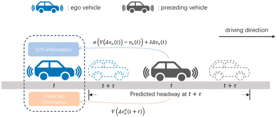
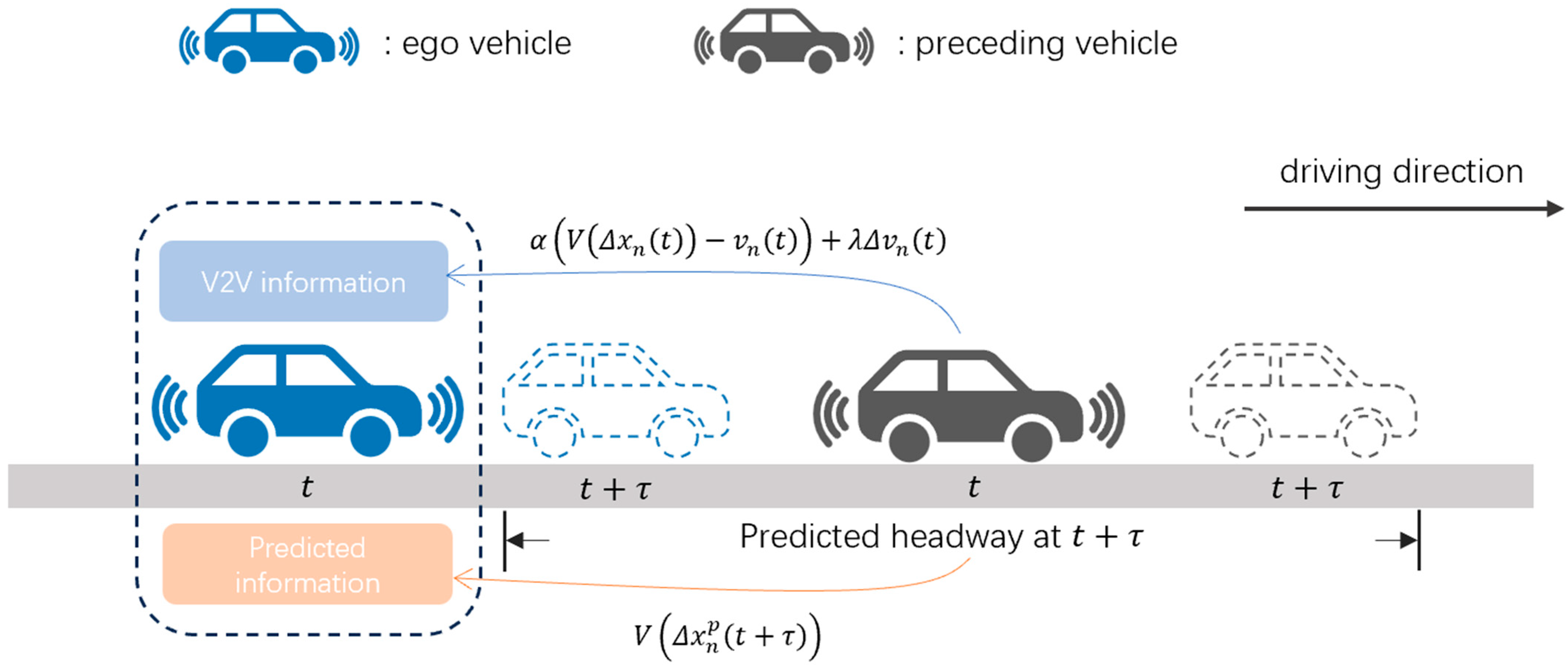
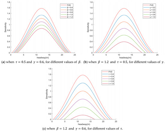
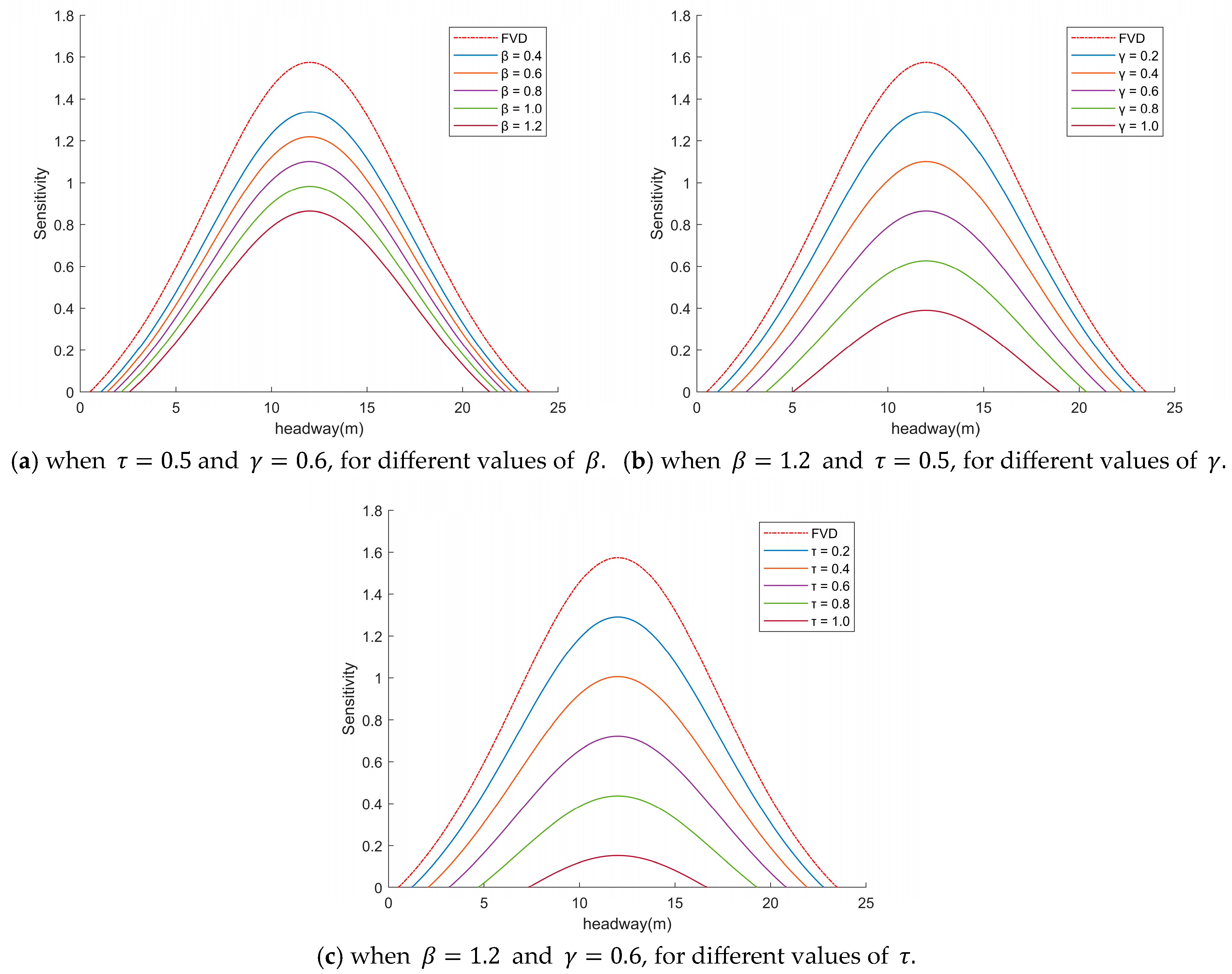
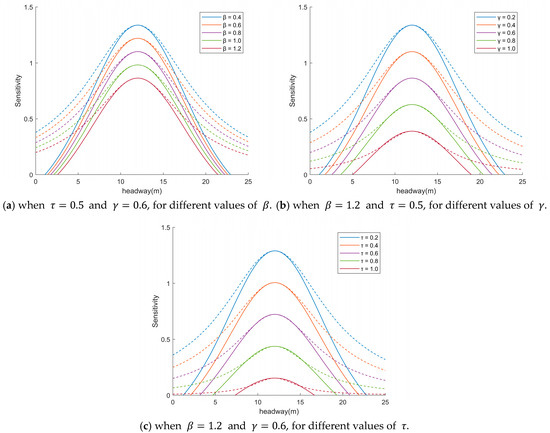
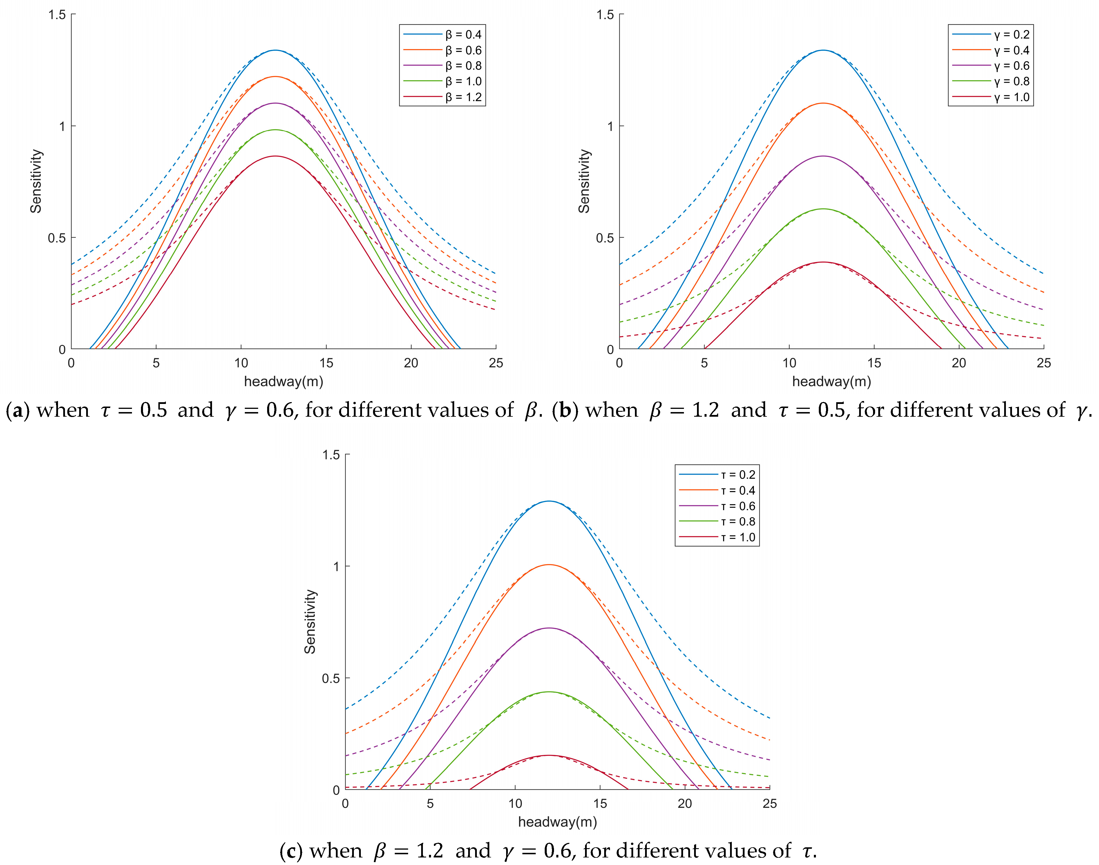
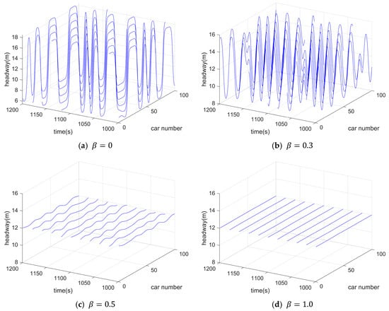
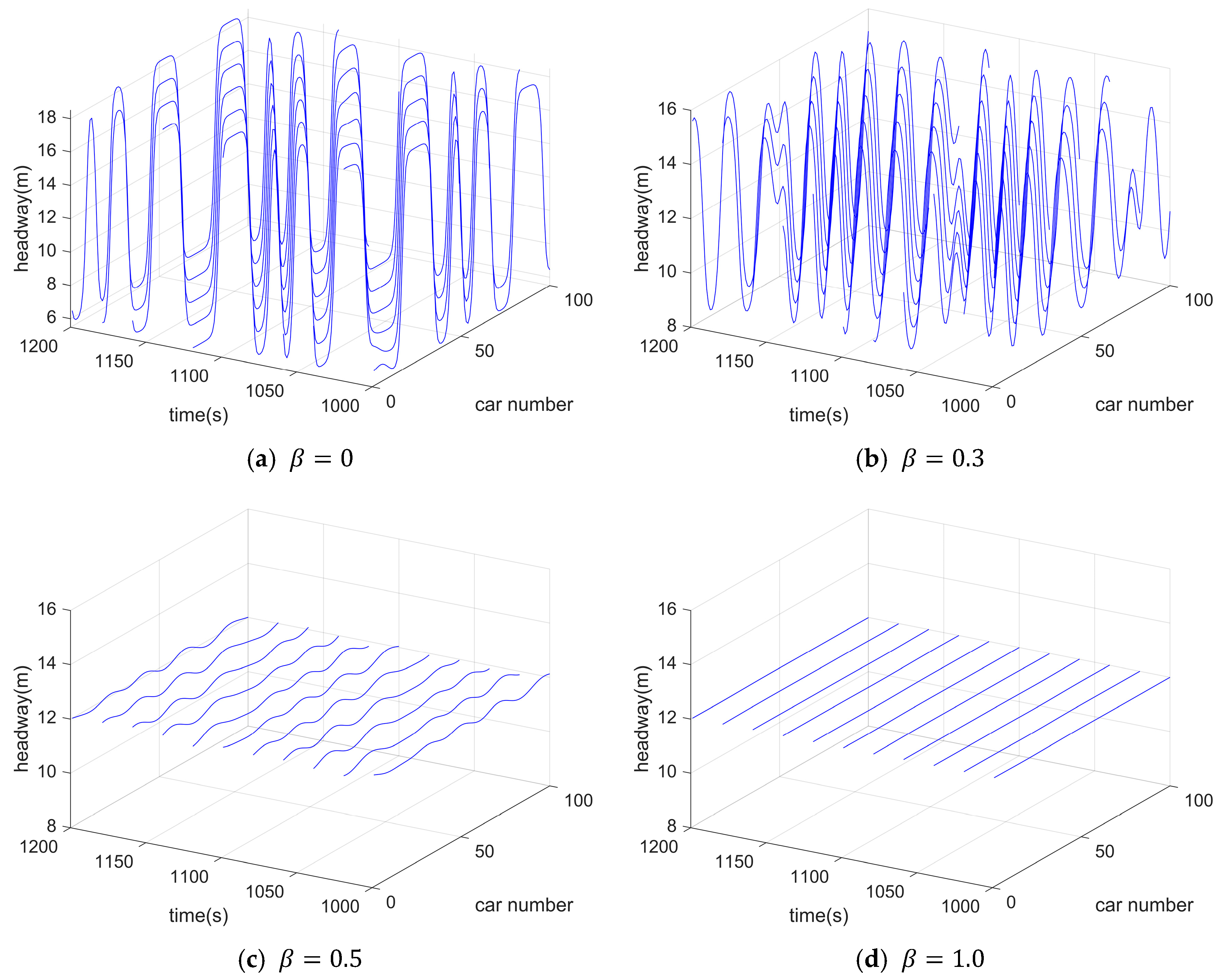
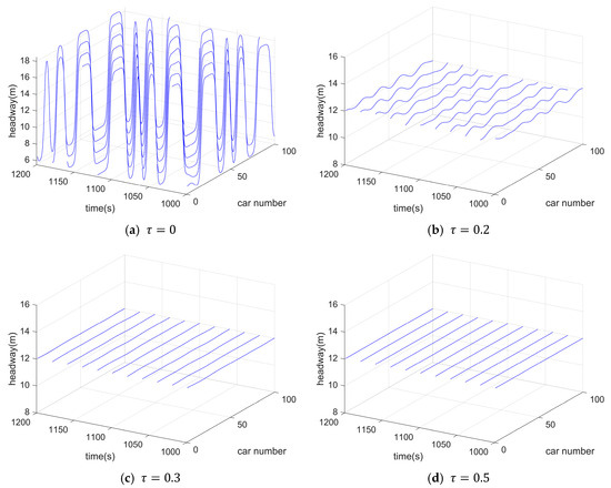
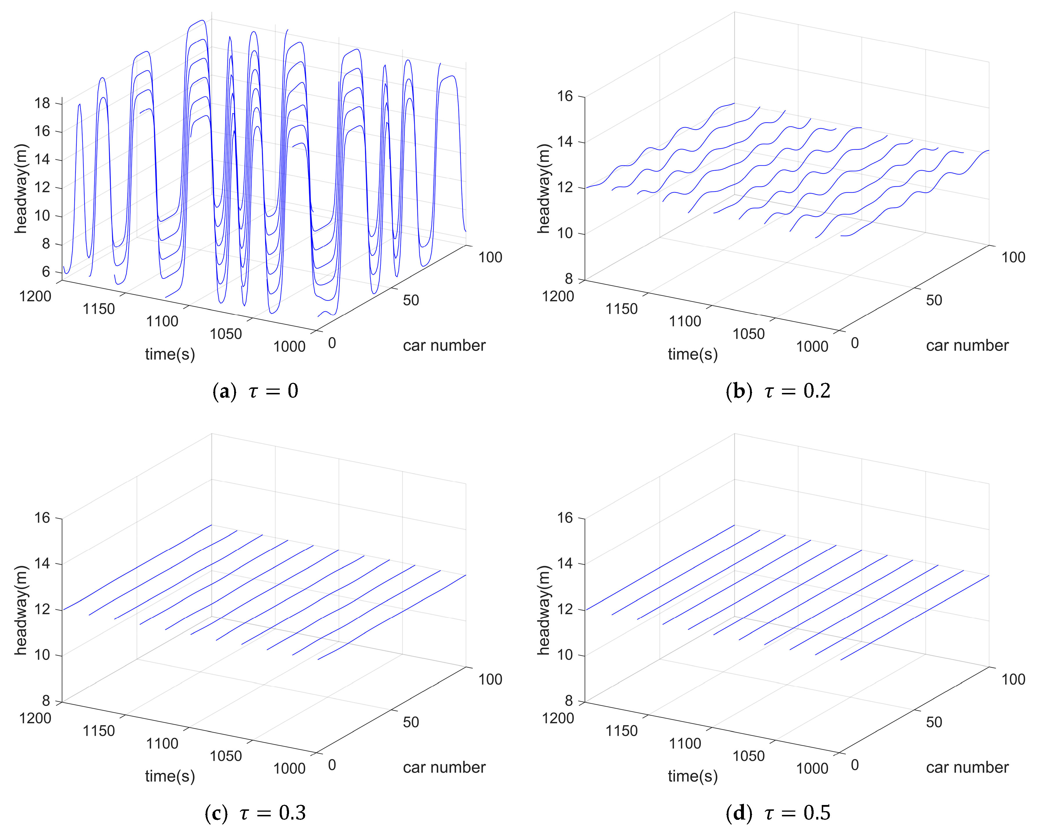
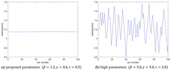
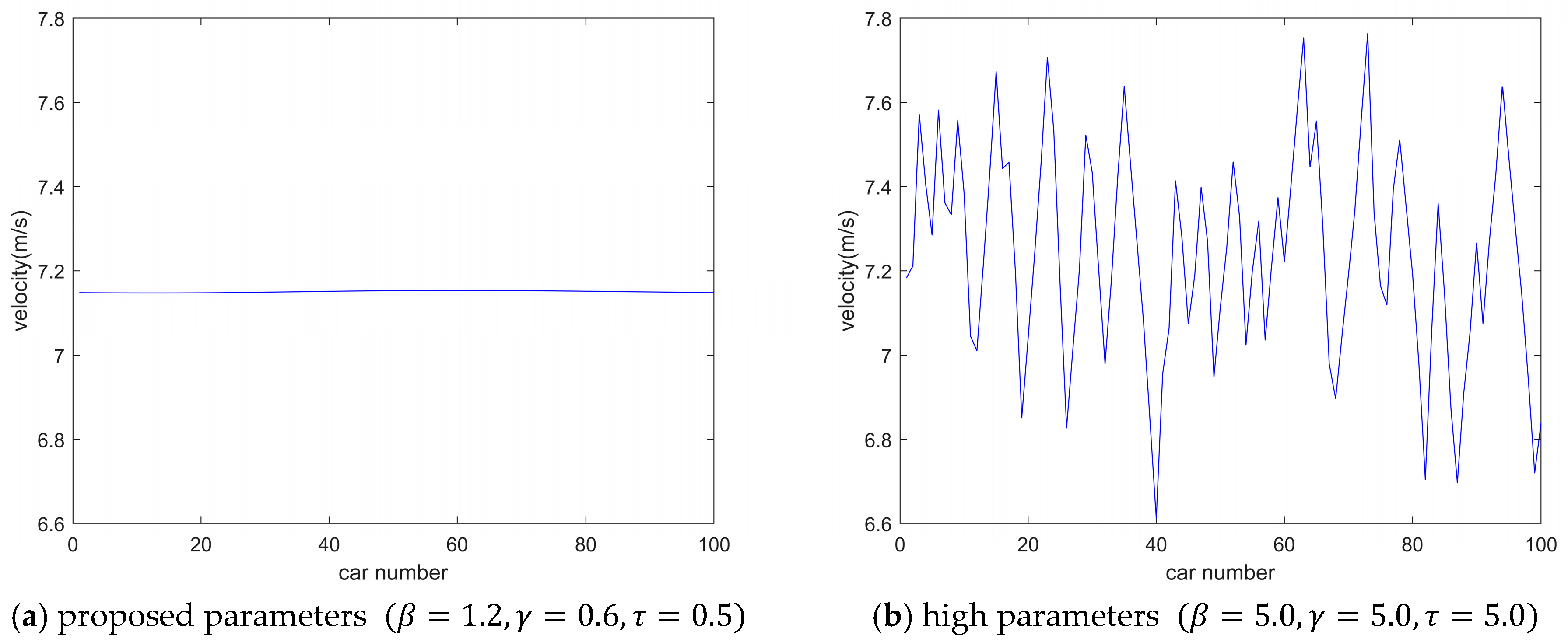
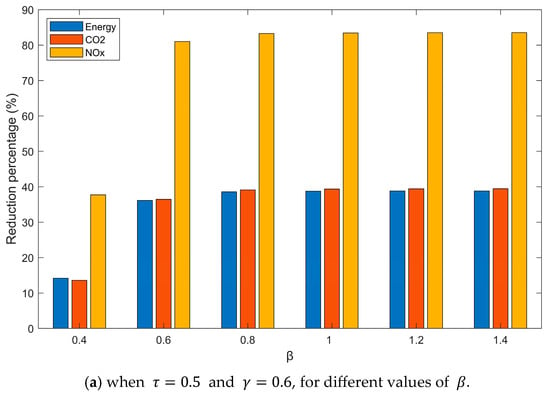
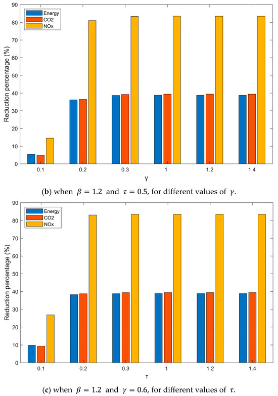
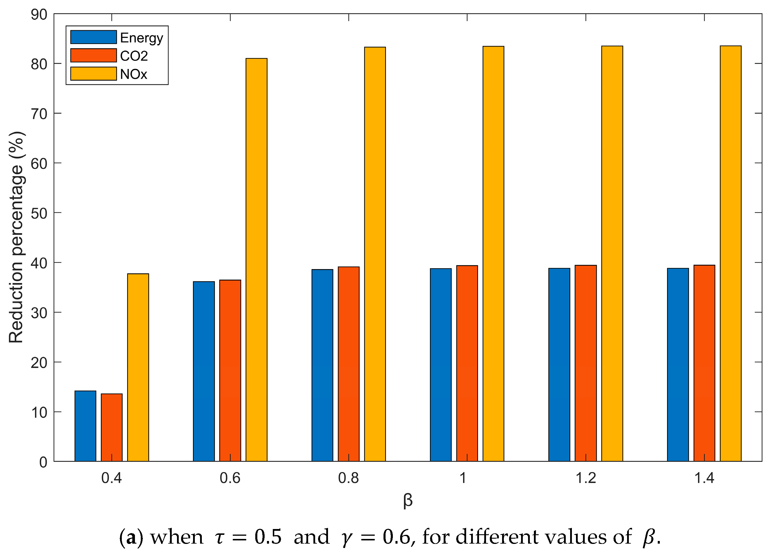
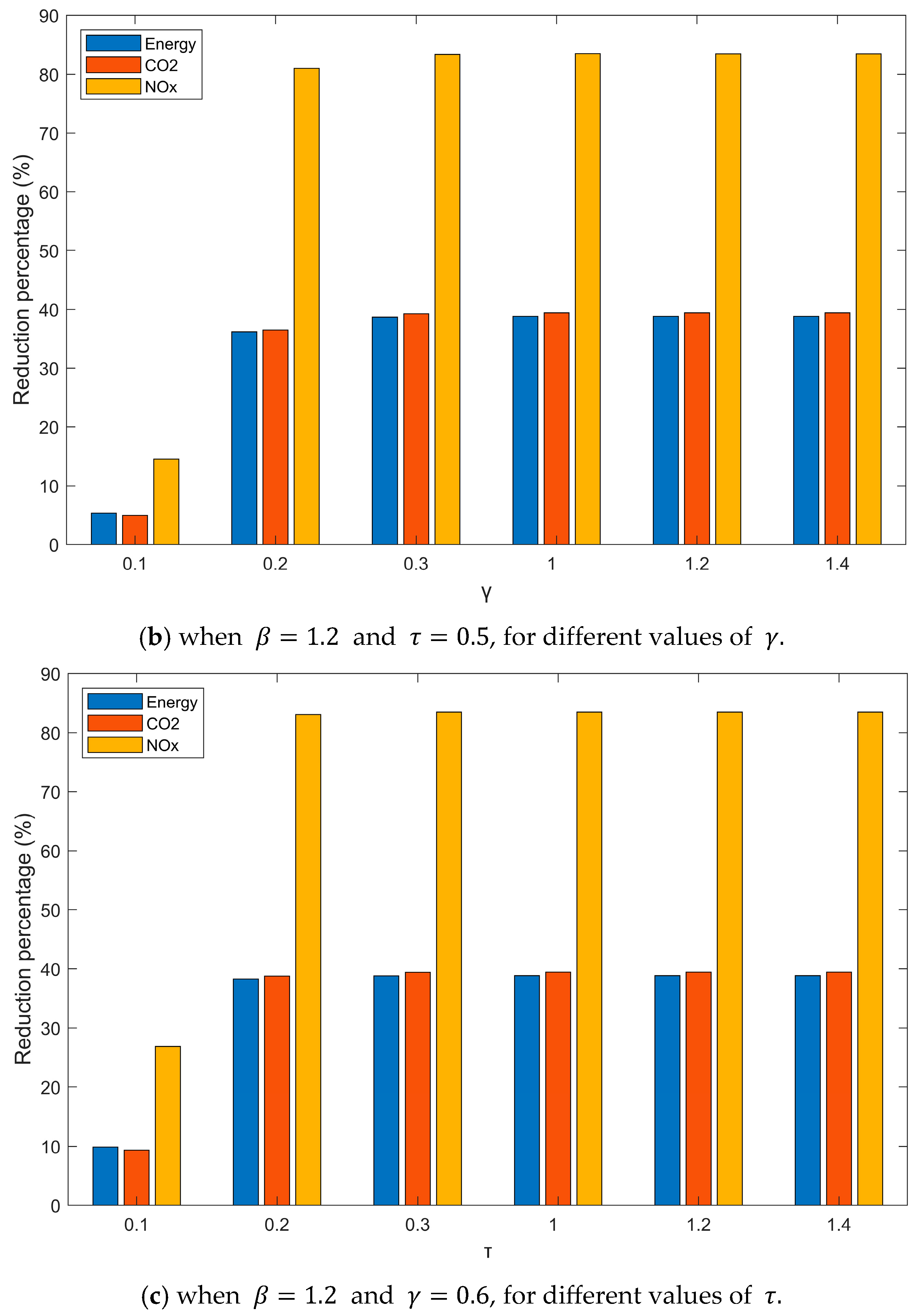
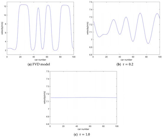
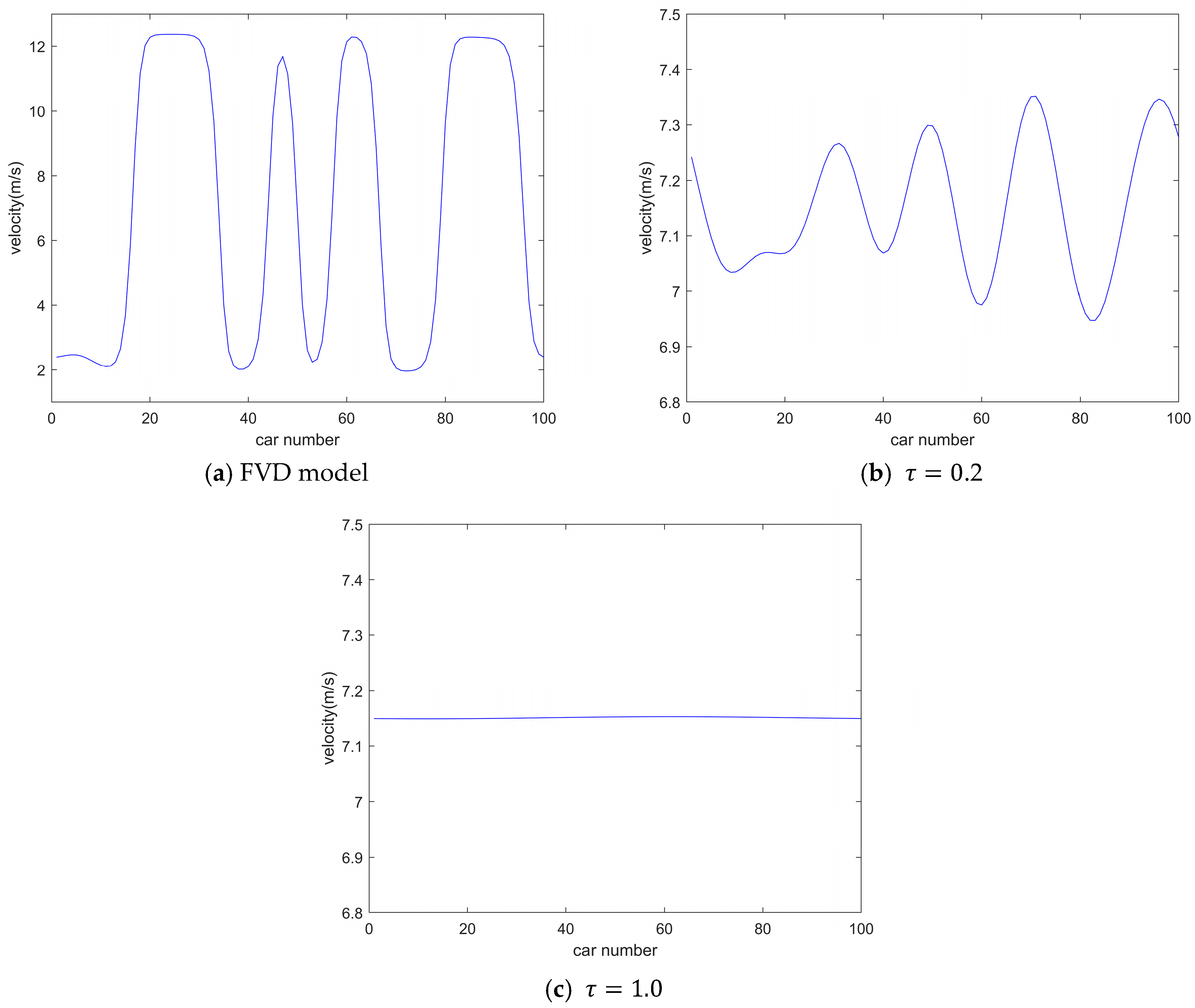
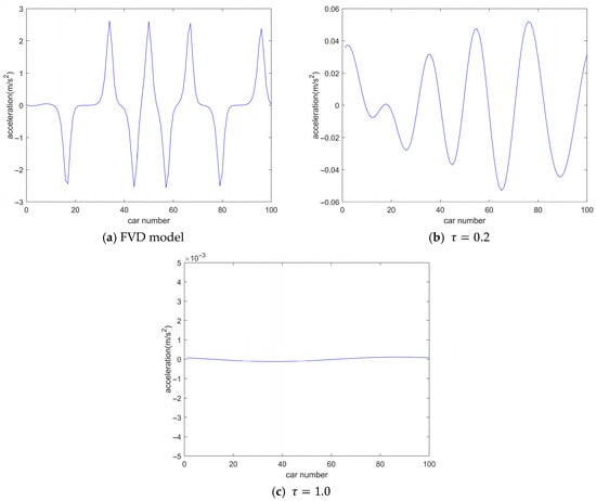
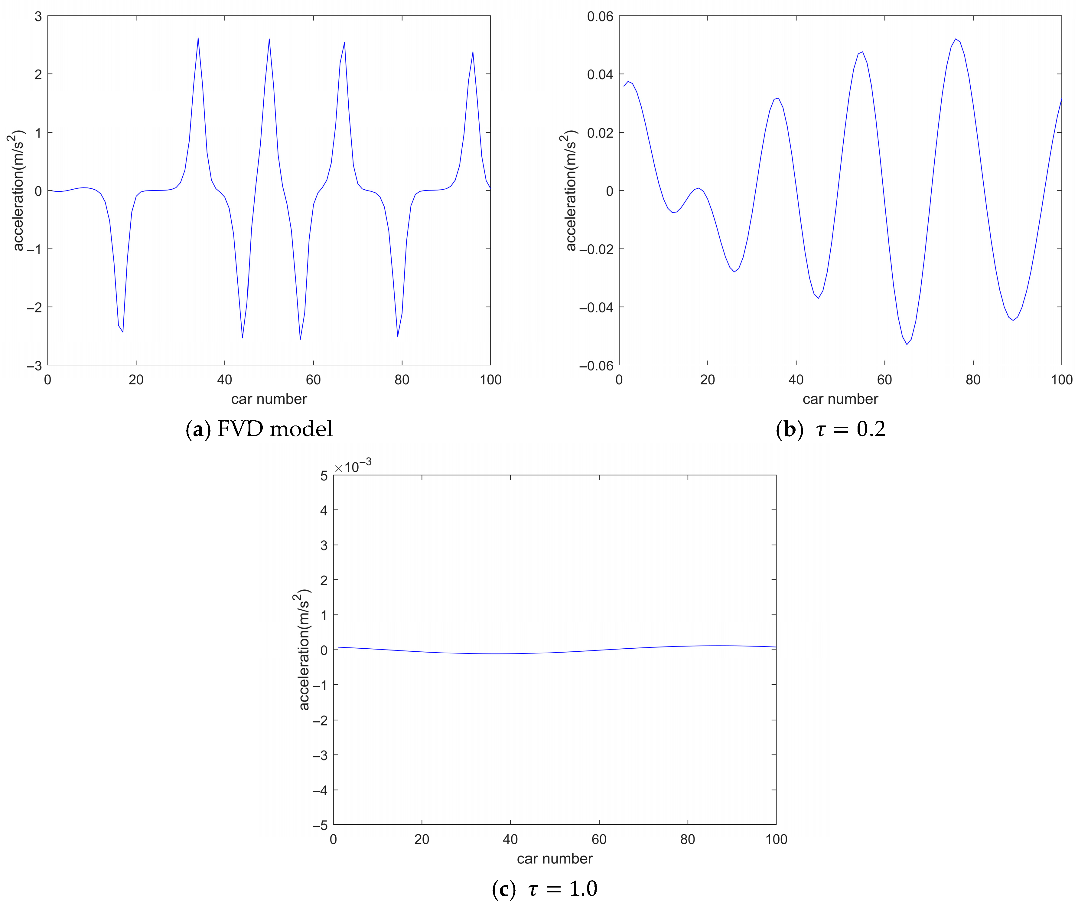

Disclaimer/Publisher’s Note: The statements, opinions and data contained in all publications are solely those of the individual author(s) and contributor(s) and not of MDPI and/or the editor(s). MDPI and/or the editor(s) disclaim responsibility for any injury to people or property resulting from any ideas, methods, instructions or products referred to in the content. |
© 2026 by the authors. Licensee MDPI, Basel, Switzerland. This article is an open access article distributed under the terms and conditions of the Creative Commons Attribution (CC BY) license.