


Abstract
To overcome the limitations of ground-based observations, this study aims to identify optimal color indices for detecting tree phenological events using time-series Unmanned Aerial Vehicle(UAV) orthomosaics. We monitored 37 woody taxa at the Korea National Arboretum from April to November 2025. By extracting Red, Green, and Blue (RGB) values from canopy polygons, we calculated four indices: Brightness, Green Chromatic Coordinate (GCC), Red Chromatic Coordinate (RCC), and Green-Red Vegetation Index (GRVI). We then evaluated signal detectability using Z-score standardization. The analysis confirmed that 74.6% of phenological events were detectable. Specifically, flowering and autumn coloration showed high detection rates (88.9% and 100%, respectively), identifying Brightness, RCC, and GRVI as key indicators for capturing these distinct visual changes. Conversely, gradual transitions like leaf-out showed lower detectability. These findings demonstrate that selecting specific color indices based on the visual characteristics of each event enables effective quantitative monitoring. This study provides a methodological basis for utilizing UAV-based indices as a complementary tool in long-term ecological monitoring.
1. Introduction
Plant phenology refers to recurrent biological events such as leaf-out, flowering, flower abscission, autumn coloration, and leaf fall, and has been utilized as a key indicator for understanding ecosystem responses to climate change [1,2]. These phenological phenomena not only reflect the growth characteristics of individual plant species but are also closely linked to variations in photosynthetic productivity, nutrient cycling, energy flow, species interactions, and the spatiotemporal dynamics of biodiversity [1,3]. Consequently, phenology is recognized as a critical component in climate change impact assessment and long-term ecological monitoring.
Traditionally, phenological research has been based on direct observation by field surveyors targeting specific plant individuals or communities. While this method of visual observation allows for the intuitive recording of phenological phenomena, it possesses structural limitations, including observer subjectivity, discontinuous observation intervals, and a high dependency on labor and time [4]. In particular, maintaining consistency in observation standards and data continuity is essential in long-term ecological monitoring systems, yet relying solely on field surveys imposes realistic constraints on sustaining this stability.
To address these limitations, phenological research utilizing satellite imagery has been actively developed since the 1970s alongside advancements in remote sensing technology [2]. Subsequently, long-term time-series analyses using vegetation indices such as Normalized Difference Vegetation Index (NDVI ) have reported earlier spring green-up and delayed autumn leaf fall on continental and global scales [5,6]. Satellite-based approaches have dramatically expanded the spatial scope of phenological research by enabling simultaneous observation of extensive areas and the utilization of long-term accumulated data. However, due to the problem of mixed signals from multiple plant species within a single pixel, there are limitations in precisely analyzing phenological changes at the level of individual trees or specific species, and issues regarding data gaps caused by clouds and observation cycles also exist [6].
Recently, research on phenology based on ultra-high-resolution imagery using Unmanned Aerial Vehicles (UAVs) has attracted attention to complement these limitations. UAV imagery provides centimeter-level spatial resolution, enabling the direct tracking of phenological changes at the individual tree canopy level, and is advantageous for quantitatively analyzing phenomena with distinct visual changes, such as leaf emergence or autumn coloration [7,8]. Some studies have reported achievements in estimating leaf-out and leaf fall dates for thousands of individual trees through automated canopy segmentation and time-series image analysis [9]. However, UAV-based observations face application limits for long-term and large-area monitoring due to costs associated with repeated flights, operational burdens, and limited coverage areas [8,10].
Meanwhile, PhenoCam-based monitoring, which involves installing digital cameras at fixed locations to continuously photograph vegetation, has spread rapidly over the past decade [11]. PhenoCams can automatically acquire images multiple times a day to continuously record minute changes in phenological phenomena, and color-based indices such as the Green Chromatic Coordinate (GCC) allow for the quantification of leaf-out, autumn coloration, and leaf fall timings [1,12]. These data show high agreement with field visual observations and satellite-based phenology products and are also used as validation data for satellite observation results [11]. However, as observation points are fixed, there is a limitation regarding spatial representativeness.
Although image-based phenology detection techniques have evolved into various forms such as satellite imagery, UAV imagery, and PhenoCams, most previous studies have been conducted on specific regions, single species, or limited observation periods. In particular, there are still limited cases that utilize repeated UAV orthomosaics for fixed individuals in natural mixed forests to detect phenological signals and directly compare them with existing visual observation results [9,10]. Under these circumstances, applying image-based techniques directly to long-term ecological monitoring systems could result in institutional decisions being made without sufficiently verifying data reliability and operational efficiency. Furthermore, since long-term ecological monitoring systems operate on the premise of consistent survey methods and stable data accumulation, a thorough review of consistency with existing survey systems is essential before introducing new technologies or analysis methods. While image-based phenology detection techniques possess clear advantages in terms of survey automation and objectivity, various factors such as shooting timing, shooting angle, illumination conditions, and differences in canopy structure can affect analysis results in actual field applications [10]. Therefore, failure to evaluate in advance how such uncertainties affect the interpretation of phenological signals poses a risk of undermining the continuity and comparability of long-term monitoring data.
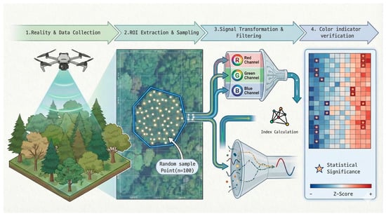
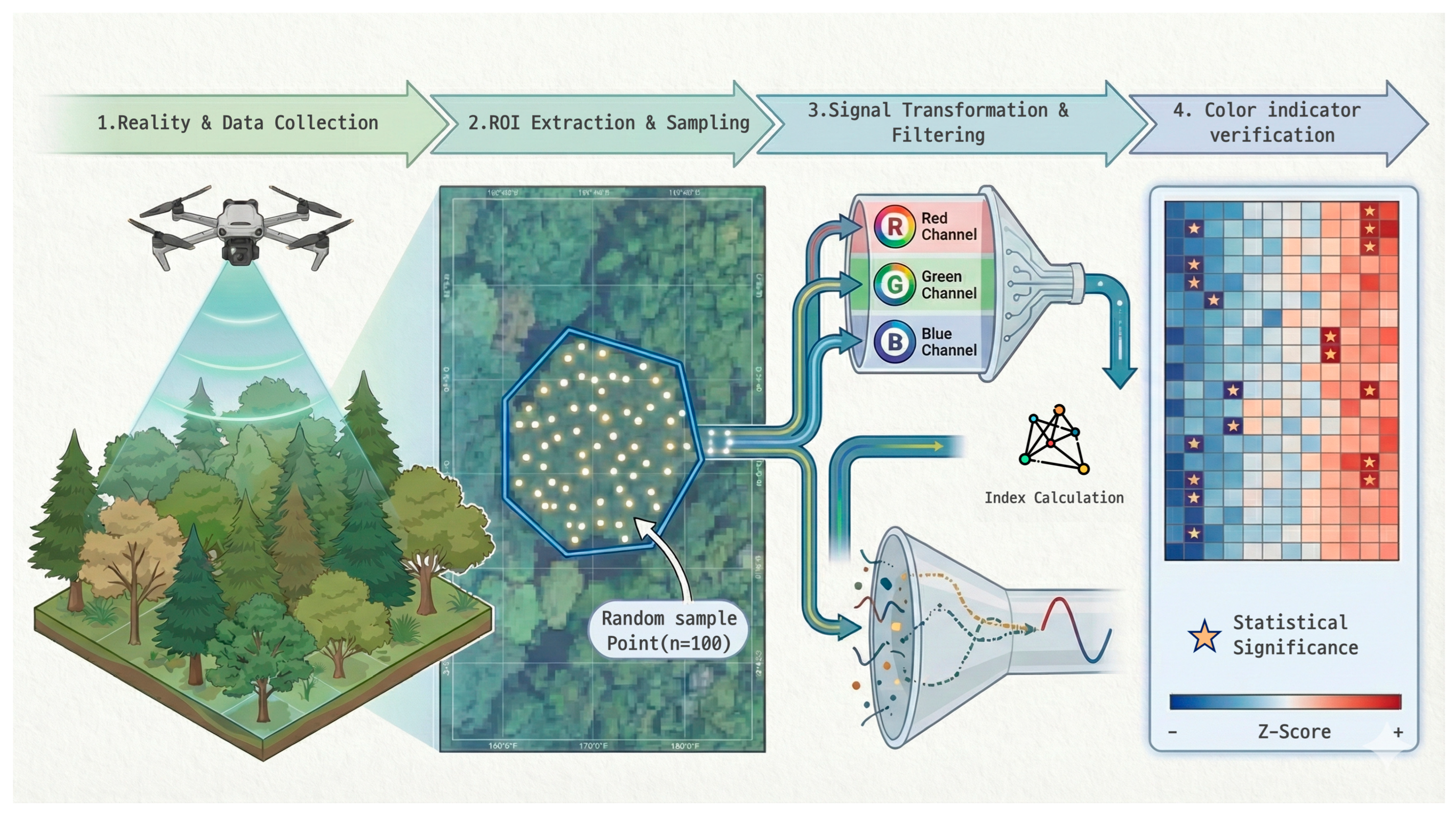
Based on the background and problem awareness presented above, this study was performed as a pilot study to evaluate the applicability of image-based phenology detection techniques within a long-term ecological monitoring framework. In particular, we focused on whether color-based indices derived from drone orthomosaics can provide objective and quantitative information that complements the existing visual observation-centered phenology survey system. The primary objective of this study is to verify whether major phenological events such as leaf-out, flowering, leaf fall, and autumn coloration are detectable as time-series color signals in drone orthomosaics for plants that maintain green canopies during the general growing season. To this end, we established an analytical framework to directly compare existing phenology records based on visual interpretation with results from image-based quantitative analysis. Specifically, canopy polygons of monitoring target trees were generated from the initially captured orthomosaic, and unique identifiers were assigned at the individual level. Subsequently, random sample points were generated within each canopy to extract irradiance-compensated RGB Digital Number (DN) values from orthomosaics captured over multiple time points. The individual canopy color time-series data constructed in this way were utilized to detect phenological events by applying color index calculations and standardized statistical analysis techniques (Figure 1). Through this approach, this study aimed to evaluate the degree of sensitivity and limitations that color-based image indices possess regarding different phenological processes. The results of this study aim to provide a methodological basis for the stepwise integration of drone-based phenology monitoring techniques into existing long-term ecological observation systems.
Figure 1.
Schematic workflow for automated detection of tree phenology using time-series orthophotos. The methodology consists of four main stages: (1) Reality & Data Collection, involving the acquisition of high-resolution time-series images using a UAV; (2) Region of Interest (ROI) Extraction & Sampling, where RGB spectral data are extracted from random points () generated within canopy polygons; (3) Signal Transformation & Filtering, which involves separating RGB channels and calculating color indices; and (4) Color indicator verification, utilizing the Z-score algorithm to isolate significant phenological signals (indicated by stars) from background noise.
2. Materials and Methods
2.1. Study Area
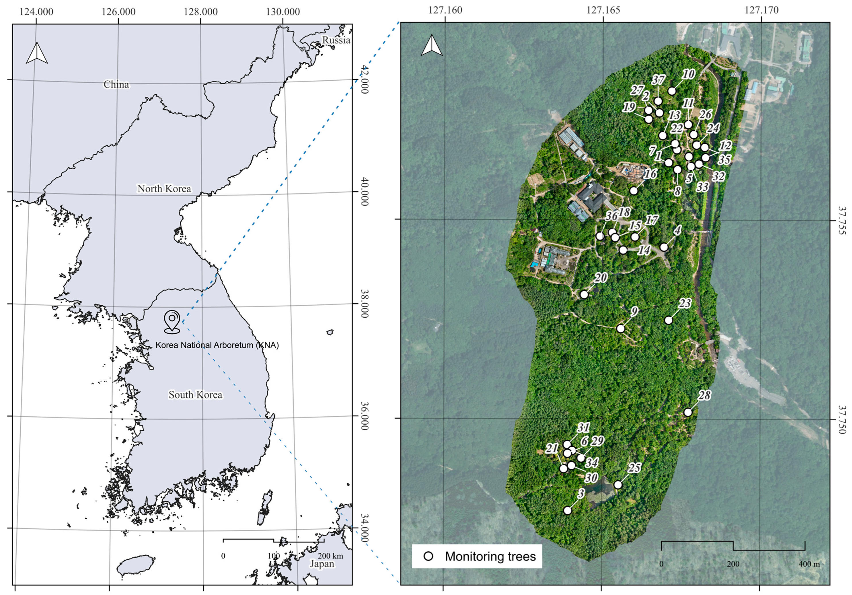
The study was conducted in Gwangneung Forest, located within the Korea National Arboretum (KNA) in Soheul-eup, Pocheon-si, Gyeonggi-do, Republic of Korea. Gwangneung Forest is a forest area of high conservation value and has been designated as a UNESCO Biosphere Reserve. The specific study site corresponds to the exhibition garden area of the KNA, covering an area of approximately 658,250 m2.
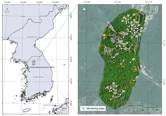
The plants selected for monitoring in this study primarily consist of woody species that have been continuously managed and observed as part of the KNA’s long-term ecological monitoring program for over a decade. Although the sample size for certain phenological events (e.g., autumn coloration) is limited by the fixed composition of these established monitoring plots, these trees offer unique value due to the continuity of historical ground truth data. Herbaceous plants were excluded from the analysis if phenological phenomena—such as flowering, leaf-out, flower abscission, leaf fall, and autumn coloration—could not be clearly identified through image interpretation. Ultimately, a total of 37 taxa were included in the monitoring analysis. The scientific name, type (e.g., evergreen conifer, evergreen broadleaf, deciduous broadleaf), and specific location of the monitoring individual tree for each taxon are presented in Figure 2 and Table 1.
Figure 2.
Location of the study area and distribution of monitoring trees at the Korea National Arboretum (KNA). The left panel shows the geographical location of the KNA within the Korean Peninsula. The right panel displays the high-resolution UAV orthomosaic of the study site, with white circles (numbered 1–37) indicating the specific locations of the individual monitoring trees used for phenological observation.
Table 1.
List of 37 monitoring tree species at the Korea National Arboretum (KNA).
2.2. UAV Data Acquisition and Orthomosaic Processing
The UAV used in this study was the DJI Mavic 3 Multispectral (M3M) model (DJI, Shenzhen, China). This aircraft is equipped with an Real-Time Kinematic (RTK) module and an incident light sensor (Green: 560 ± 16 nm, Red: 650 ± 16 nm, Red Edge: 730 ± 16 nm, NIR: 860 ± 26 nm) that records solar irradiance in real-time to compensate for illumination changes during flight. This UAV ensures consistent positional accuracy during repeated flights based on identical flight paths and allows for the correction of varying solar irradiance conditions on different shooting dates.
UAV data acquisition was conducted from 11 April 2025 to 1 November 2025. The shooting interval was set to twice a month during the general growing season (July–September), when no distinct phenological changes occur in the monitoring target plants. However, during periods of major phenological events, such as leaf-out/flowering and autumn coloration/leaf fall, the frequency was increased to four times a month.
The flight altitude was maintained at approximately 65 m above ground level (AGL) using the terrain-following mode. This altitude was determined as the minimum safe height considering obstacles such as transmission lines and communication towers. All flights were fixed at 10:00 AM to minimize shadow effects caused by changes in solar elevation.
The total number of flight days during the study period was 23. The schedule reflected operational constraints, such as the weekly closure of the KNA Exhibition Garden on Mondays and safety regulations limiting flights to a maximum of once per week to prevent accidents. The captured images were processed using DJI Terra software (v.4.25, DJI, Shenzhen, China) for stitching and orthorectification. Radiometric processing was conducted using the software’s internal algorithms, utilizing the irradiance data captured by the incident light sensor. This process compensated for lighting variations across images, generating irradiance-compensated RGB Digital Number (DN) orthomosaics suitable for time-series trend analysis. The average spatial resolution of the generated orthomosaics is approximately 0.023 m (see Figure 2 for a representative orthomosaic).
2.3. Ground Truth: Field Phenological Observations
To validate the UAV-based detection, ground-based phenological surveys were conducted synchronously with the UAV flights. To minimize observer subjectivity and ensure data reliability, two trained researchers performed the field surveys simultaneously on each shooting date. The phenological status of each tree (e.g., onset of flowering, peak autumn coloration) was recorded only when a consensus was reached between the two observers, following the standardized protocols of the KNA long-term monitoring system.
2.4. Extraction of Color Values from Monitoring Plants
The primary objective of this study is to detect representative phenological events—such as flowering, leaf-out, flower abscission, leaf fall, and autumn coloration—in plants that maintain green foliage during the general growing season [2]. To achieve this, we performed a time-series analysis by extracting RGB band information from orthomosaics, enabling mutual comparison and verification between visual interpretation results and quantitative analysis data [11].
First, canopy polygons were generated based on the canopy area of the monitoring target trees from the initial orthomosaic, and a unique ID (including species name) was assigned to each polygon for individual identification. This canopy-level analysis approach is widely used as a standard method for precisely tracking phenological changes at the individual tree level [13].
Subsequently, 100 random points were generated within each canopy polygon as samples for extracting color values. Instead of using all pixels within the canopy area, we applied this random sampling method to maintain statistical representativeness of the color distribution within the canopy while reducing visualization density and computational load [6]. Based on these generated random points, RGB Digital Number (DN) values were extracted from the orthomosaics at each shooting timestamp, thereby constructing time-series data of RGB color values for each monitoring tree. The constructed time-series color data were then utilized for phenological event detection analysis using color index calculations and Z-score-based outlier detection techniques [12,14].
2.5. Analysis of RGB DN Value Deviations
This phase serves as a preliminary analysis to determine whether RGB DN values observed on specific dates represent statistically significant signals compared to the plant’s overall time-series color fluctuation range. The purpose is to verify whether a color change constitutes a “detectable phenological event” distinct from general fluctuations caused by solar conditions or seasonal trends, prior to applying standardized quantitative detection indices such as Z-scores.
We specifically targeted the G-band DN values extracted from the random points. This is because the G-band is highly sensitive to vegetation dynamics: green reflectance distinctively increases with rising chlorophyll content during growth and decreases during chlorophyll degradation in autumn coloration and leaf fall processes [15]. Furthermore, during flowering, the proportion of non-green elements within the canopy increases, leading to a temporary reduction in green reflectance, which is also effectively captured by G-band signals [16]. Due to these characteristics, the G-band serves as an effective indicator for capturing key phenological events such as leaf-out, growth, flowering, and senescence.
Let denote the G-band DN value during the observation period . The reference value representing the average color state of the plant was calculated as follows:
To quantify the “routine color fluctuation range” resulting from changing illumination conditions or seasonal trends, the standard deviation of the G-band DN values () was calculated:
Subsequently, defining as the G-band DN value on a specific date identified as a phenological event through visual interpretation, the deviation from the mean () was calculated:
If the deviation of the G-band DN value on the event date exceeded the routine fluctuation range—that is, if the condition was met—the color change on that date was considered a statistically significant signal beyond the general range of variation. Such signals are unlikely to be explained by simple illumination changes or gradual seasonal trends and were judged as high-probability points for phenological events like leaf-out, flowering, autumn coloration, or leaf fall.
The analysis of RGB DN value deviations performed in this step quantitatively validates how exceptional the phenological event was compared to the average growth state. It provides the theoretical and statistical basis for the subsequent Z-score-based standardization analysis. This ensures that the Z-score analysis functions not merely as a numerical transformation, but as a quantitative event detection stage targeting signals whose detectability has been statistically verified.
2.6. Selection of Phenological Event Indicators
Building upon the confirmation that phenological events can be detected using orthomosaics through the G-band deviation analysis, we selected normalized color indices combining RGB values as event indicators to ensure more stable detection [1,15]. By normalizing each band value against the total brightness (R + G + B) rather than using raw RGB values, these indices minimize the influence of varying solar illumination conditions or exposure differences across shooting timestamps, thereby effectively extracting intrinsic canopy color information.
Normalized RGB color indices have been widely utilized as effective metrics for detecting major phenological events—such as leaf-out, growth, flowering, autumn coloration, and leaf fall—in digital repeat photogrammetry and remote sensing-based phenology research. Based on these preceding studies, we selected four key color indices sensitive to phenological detection as event indicators for this study (Table 2).
Table 2.
Color-based indices used for phenological event detection.
2.7. Statistical Verification of Indicator Significance
To verify the statistical significance of the color-based detection indices calculated in Table 2, we applied the Z-score (standard score) method. The Z-score is a statistical metric that expresses how far a specific observation deviates from the mean in units of standard deviation. It is utilized in time-series data to determine whether a value at a specific point falls within the range of general variation.
In this study, the period during which no phenological events occurred was defined as the “growing season.” Based on this period, the mean and standard deviation of each color index were calculated. The mean ( and standard deviation () during the growing season are defined as follows:
where represents the color index value observed at time point , and denotes the total number of observation points corresponding to the growing season.
Subsequently, the color index value at each time point observed across the entire time series was standardized into a Z-score based on the growing season mean and standard deviation:
This process allows for a quantitative evaluation of how anomalous the color change at each time point is compared to the average growth state.
In this study, a Z-score exceeding ±2 (i.e., ) was considered a statistically significant change that deviates from the general range of variation [19]. Assuming a normal distribution, this threshold corresponds to outliers falling outside approximately 95% of the total observations and has been used as a universal threshold for identifying abnormal events in time-series data.
Color changes detected in this manner are interpreted as variations difficult to explain by simple illumination changes or gradual seasonal trends, and were judged as high-probability points where major phenological events—such as leaf-out, flowering, autumn coloration, and leaf fall—occurred. Through this Z-score-based significance verification, phenological events with statistical detection value were identified from the color index time series according to objective criteria.
2.8. Use of AI Tools
In the preparation of this manuscript, the authors utilized generative AI tools to assist with data analysis, visualization, and language refinement. First, AI-based coding assistants were employed to implement the analysis logic and optimize the R scripts used for extracting RGB values and calculating Z-scores. Second, the schematic illustration of the research workflow presented in Figure 1 was initially generated using a text-to-image AI tool and subsequently refined by the authors to accurately reflect the study design. Finally, as the authors are non-native English speakers, Large Language Models (LLMs) were used for English translation and grammatical editing to improve the clarity and readability of the manuscript. The authors reviewed and verified all AI-generated content, code, and text to ensure accuracy and take full responsibility for the final output.
3. Results
3.1. Visual Interpretation of Phenological Events Based on Time-Series RGB Band Responses from Orthomosaics
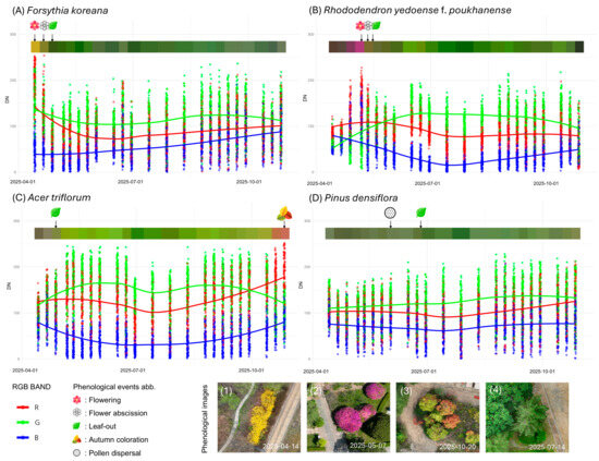
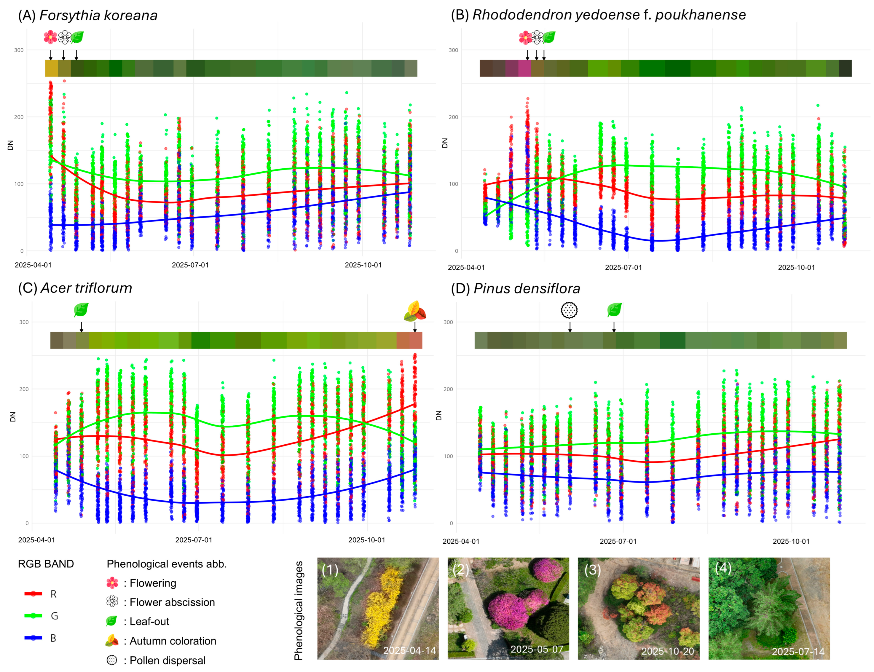
We integrated and visualized the distribution of RGB Digital Number (DN) values extracted from random points within the canopy polygons of monitoring trees from time-series orthomosaics, along with ground-based visual observation data and temporal composite colors. This approach ensured intuitive interpretation of phenological events corresponding to RGB changes. Figure 3 presents a comparison of time-series responses for representative species exhibiting distinct color changes among the studied taxa: flowering species (Forsythia koreana, Rhododendron yedoense f. poukhanense), an autumn coloration species (Acer triflorum), and an evergreen control species (Pinus densiflora).
Figure 3.
Characterization of time-series RGB band responses and comparison with orthomosaics. This figure visualizes the distribution and trends of time-series RGB DN values for four species representing key phenological events: (A) Forsythia koreana (Flowering), (B) Rhododendron yedoense f. poukhanense (Flowering), (C) Acer triflorum (Autumn coloration), and (D) Pinus densiflora (Evergreen control). Each panel consists of raw data points extracted from random sampling locations (dots) and smoothed trend lines (solid lines). The upper color bar represents the average canopy color at each observation date. Arrows and icons indicate the timing of phenological events observed during ground surveys, while the bottom images (1–4) display actual orthomosaics captured during the peak expression of phenology for each species.
The analysis revealed that RGB band response patterns were clearly distinguished according to the unique leaf and flower colors of each species.
First, Forsythia koreana, which produces yellow flowers in early spring, showed a tendency for both Red (R) and Green (G) band values to remain high as the canopy was covered in yellow during the flowering period. This is confirmed by the distinct yellow canopy in the orthomosaic displayed at the bottom of Figure 3A.
Second, for Rhododendron yedoense f. poukhanense, the R-band values rose sharply relative to the G-band as magenta flowering progressed, forming a distinct peak (Figure 3B).
Third, Acer triflorum, a representative species for autumn foliage, maintained a stable time-series distribution due to green leaves during the growing season. However, during the autumn coloration period, it exhibited a crossover pattern where R-band values increased rapidly while G-band values decreased, demonstrating spectral characteristics distinct from the normal state (Figure 3C).
Conversely, the evergreen conifer Pinus densiflora showed no significant numerical fluctuation or distinct signal response in the orthomosaic-based RGB time series, despite biological events such as pollen dispersal being visually observed (Figure 3D).
These results suggest that time-series color information from UAV orthomosaics is effective in capturing visually distinct phenological events as quantitative signals.
3.2. Assessment of Phenological Signal Detectability in G-Band Time-Series and Validation of the Z-Score Approach
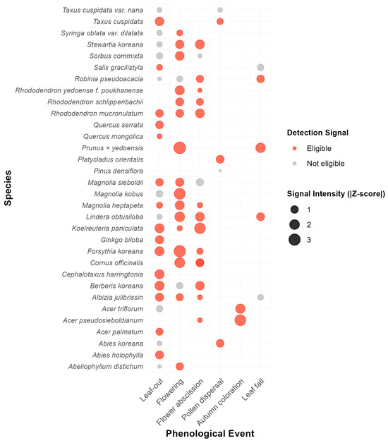
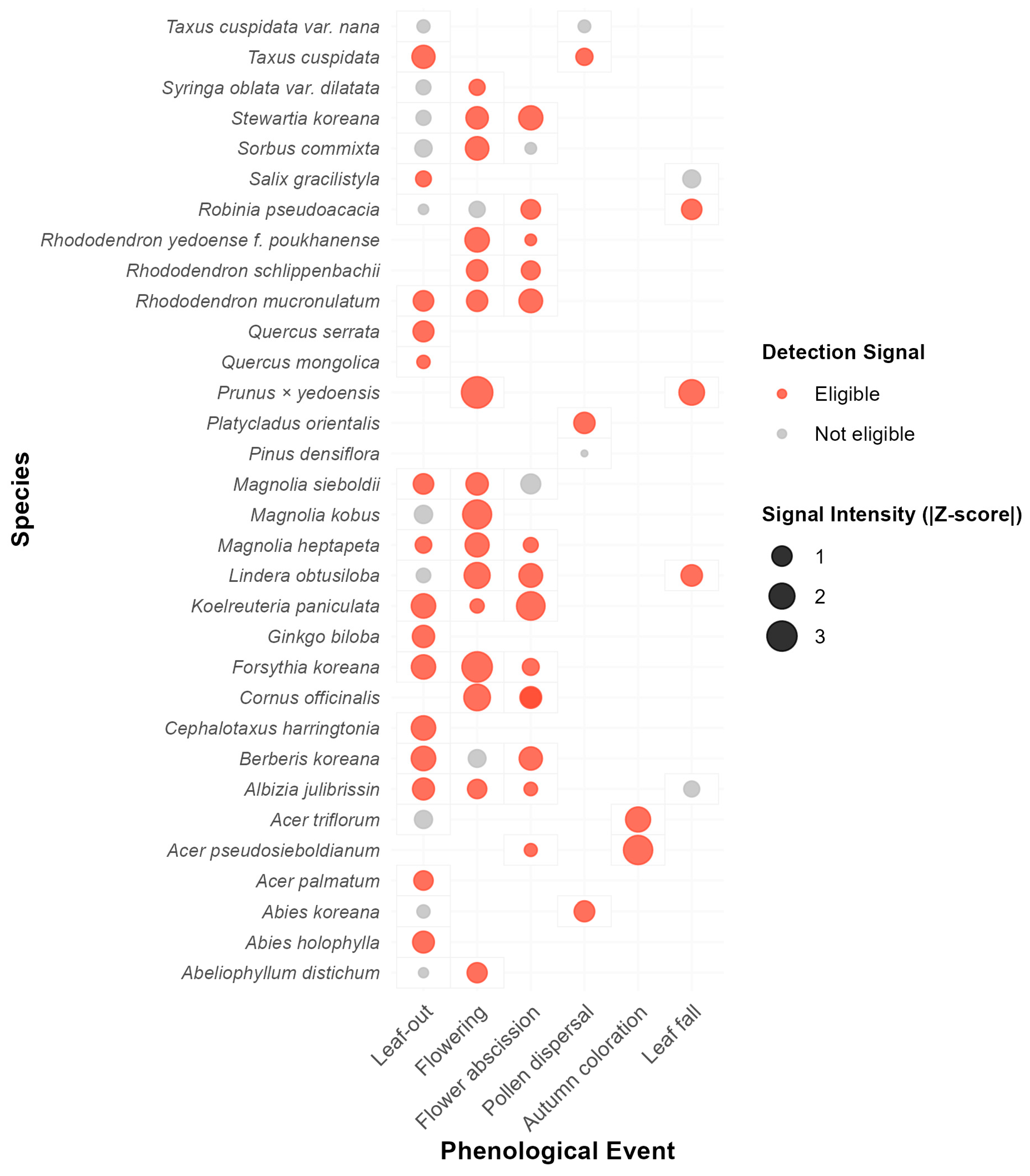
To assess whether phenological events can be detected as significant signals within the G-band time-series of digital imagery, we analyzed 71 observed events by comparing the G-band deviation on the event date against the baseline standard deviation (SD). The analysis revealed that approximately 74.6% (53 events) of the total events exhibited valid detection signals (“Eligible”) that exceeded the range of routine background noise (Figure 4).
Figure 4.
Evaluation of phenological signal detectability in G-band time-series. This matrix illustrates the detectability of seasonal events across different plant species (y-axis) and phenological stages (x-axis). The bubble size represents the signal intensity, calculated as the absolute deviation on the event day relative to the baseline SD, which corresponds to the magnitude of the Z-score. Orange bubbles (“Eligible”) indicate events where the signal exceeds the 1.0 SD threshold, justifying the feasibility of automated phenophase detection using Z-score algorithms. Gray bubbles (“Not eligible”) represent signals that fall within the range of natural baseline variability.
When examining specific phenological phases, autumn coloration (100%), flowering (88.9%), and flower abscission (87.5%) recorded high eligibility rates, demonstrating that G-band variations associated with these events are highly distinct. Notably, during the flowering period of Prunus × yedoensis, the G-band deviation reached a maximum Signal-to-Noise Ratio (SNR) of 3.31 times the baseline variability. Strong signals were also observed in Forsythia koreana (SNR 3.05) and Acer pseudosieboldianum (SNR 2.75).
In contrast, the leaf-out and leaf fall stages showed relatively lower signal intensity, with approximately 60% of events deemed eligible. This suggests that G-band fluctuations during these periods may occur at magnitudes similar to those of vegetative growth or environmental baseline variability. However, the overall results indicate that numerical variations in the G-band during phenological events statistically overwhelm background noise. This provides objective justification for the subsequent application of the Z-score-based automated detection algorithm to precisely identify phenological phases (Table 3 and Table S1).
Table 3.
Summary of G-band signal detectability and eligibility for Z-score analysis by phenological event.
3.3. Exploration of Phenological Event Detection Indicators Using Z-Scores
In this section, we explored the optimal indicators for quantitatively detecting phenological events for each species using the standardized Z-scores of the four color indices extracted from orthomosaics. The analysis revealed that the efficiency of detection indicators and the range of significant Z-scores varied depending on the unique morphological characteristics and physiological stages of the species.
3.3.1. Comprehensive Overview of Indicator Exploration via Heatmap Analysis
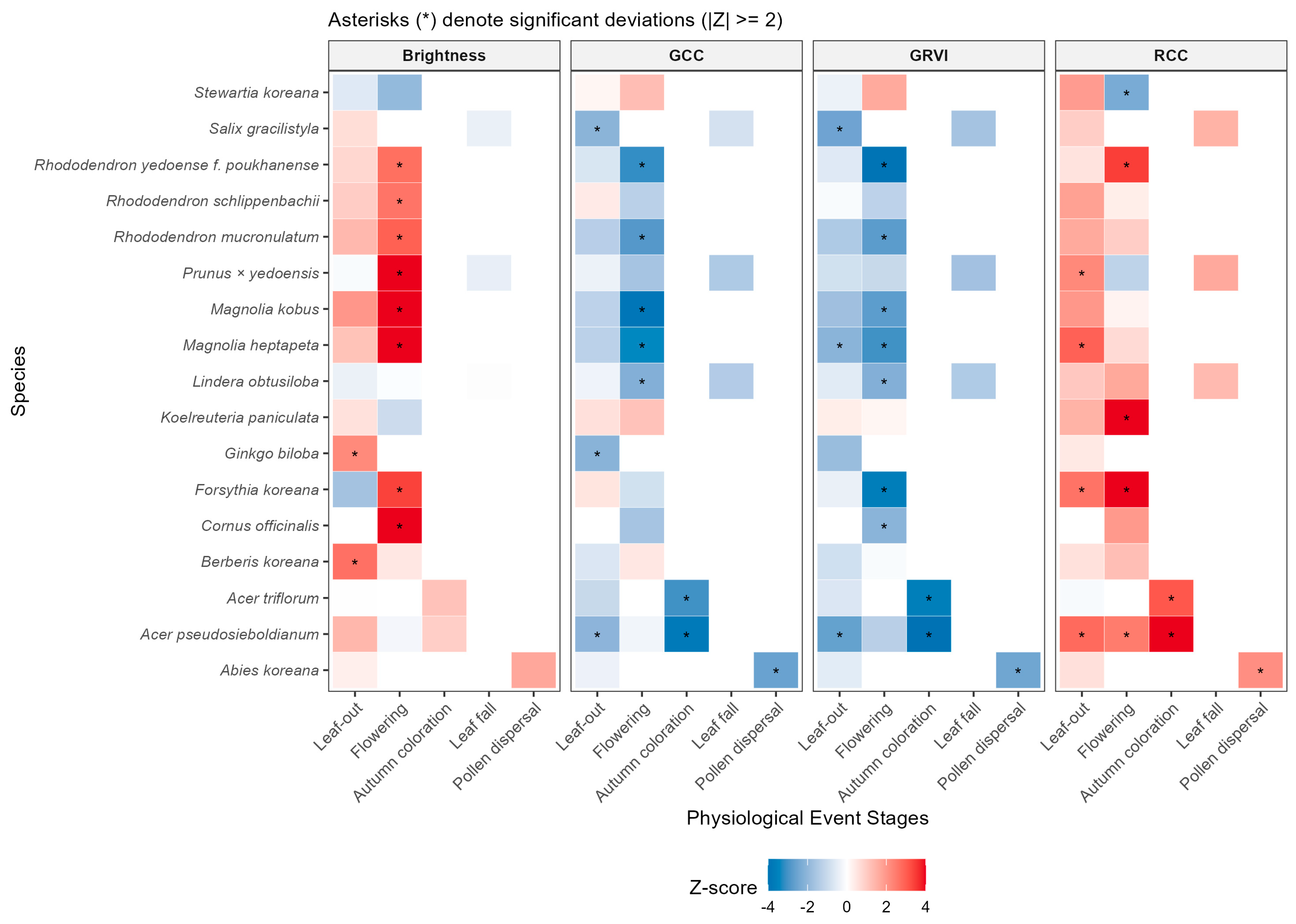
The heatmap analysis of all 37 species (Figure 5) summarizes the response patterns of each index for detecting specific events in orthomosaics as follows:
- Detection Significance: The points marked with an asterisk (*) within the heatmap cells denote This indicates that the corresponding index serves as a statistically valid “detection indicator” for the specific phenological event of that species.
- Characteristics by Indicator: GCC and GRVI generally showed high performance in detecting leaf color changes during the leaf-out and leaf fall stages. In contrast, Brightness and RCC demonstrated specialized patterns in capturing specific visual features during the flowering and autumn coloration stages.
Figure 5.
Heatmap of standardized vegetation index Z-scores by species and phenological stages derived from orthomosaics. Each cell represents the standardized deviation (Z-score) of the index relative to the baseline (growing season), where red and blue gradients indicate positive and negative shifts, respectively. The x-axis follows the ecological sequence of physiological response stages (Leaf-out, Flowering, Autumn coloration, Leaf fall, and Pollen dispersal), while the y-axis lists the studied species in alphabetical order of their scientific names. Asterisks (*) within cells denote significant deviations exceeding the detection threshold of . The four panels (Brightness, GCC, GRVI, and RCC) represent distinct optical characteristics, serving as a basis for identifying optimal indicators for specific species and phenological events.
3.3.2. Representative Examples of Detection Indicators and Z-Scores by Major Species
Detailed detection values for all species are provided in the Supplementary Materials. This section describes representative cases demonstrating the feasibility of detection using orthomosaics:
- Case 1: Acer triflorum (Autumn Coloration Detection)
- Optimal Indicators: RCC, GCC, GRVI
- Detection Range: During autumn coloration, the RCC index rises sharply to approximately 3.09, whereas GCC ( ) and GRVI () record significant negative values. This implies that the distinctive red autumn foliage of Acer triflorum can be clearly identified through cross-validation of multiple indices in orthomosaics.
- Case 2: Prunus × yedoensis (Flowering Detection)
- Optimal Indicator: Brightness
- Detection Range: The Z-score for Brightness reaches approximately 4.16 during the flowering period. This reflects the high reflectance of white flowers captured in the orthomosaic, making the brightness index a powerful detection criterion capable of isolating flowering areas within the canopy.
- Case 3: Acer pseudosieboldianum (Multi-Stage Detection)
- Optimal Indicators: RCC, GRVI
- Detection Range: High positive Z-scores were observed in both flowering ( and autumn coloration () stages. This suggests that while the same index is utilized, events can be distinguished by applying different thresholds for each period.
- Case 4: Ginkgo biloba (Leaf-out Detection)
- Optimal Indicator: Brightness.
- Detection Range: The Brightness index increases to approximately 2.22 during early leaf-out, allowing for the quantification of leaf emergence timing through changes in canopy luminance.
The optimal indicators and detailed Z-score statistics derived from this analysis for each species and event serve as baseline data for establishing remote monitoring systems using orthomosaics. For detailed numerical tables for all species, refer to Table S2 in the Supplementary Materials.
4. Discussion
4.1. Feasibility of Detecting Phenological Events Using UAV Orthomosaic-Based Color Indices
The results of this study indicated that approximately 74.6% of the 71 total phenological events exhibited significant responses where G-band time-series signals exceeded the baseline variability. This suggests that color information derived from UAV orthomosaics contains signals actually associated with phenological events, rather than merely reflecting changes in shooting conditions or seasonal trends [20,21]. In particular, very high detection eligibility was confirmed for flowering (88.9%) and autumn coloration (100%) stages. This is interpreted as a result of the rapid changes in the optical characteristics of the entire canopy—such as distinct floral coloration or leaf senescence—being effectively reflected in RGB-based image indices [22].
These findings demonstrate that, unlike satellite-based approaches centered on vegetation indices like NDVI, UAV orthomosaics can directly capture visual changes occurring at the individual tree canopy level [23,24]. The UAV-based approach possesses the strength of precisely recording how phenological phenomena manifest through changes in canopy color and structure, rather than estimating physiological state changes via indirect indices. This aligns with the validity of RGB color indices reported in PhenoCam-based studies [1,11,25]. Furthermore, this study suggests that high-resolution UAV imagery serves as a potential means to bridge the spatial and resolution gap between fixed-point camera observations and satellite imagery [9,26], thereby becoming a useful tool for linking multi-scale data in long-term ecological monitoring.
4.2. Interpretation of Differences in Detection Performance by Phenological Event Type
Distinct differences in image-based detection performance were observed depending on the type of phenological event. While very strong color signals were observed during autumn coloration and flowering phases due to rapid canopy color changes, relatively lower detection eligibility (approximately 60%) was shown for leaf-out and leaf fall stages. This is likely because leaf-out and leaf fall are “transition processes” that progress gradually over days to weeks, resulting in signals that overlap with gradual color changes or solar irradiance variations occurring throughout the growing season [23,27]. In other words, these stages are closer to gradual processes rather than distinct “events,” making it difficult to clearly distinguish their onset or offset points based on color changes at a single time point.
Meanwhile, biologically significant phenomena such as pollen dispersal in evergreen conifers, which were clearly identified in visual observations, were not captured as significant signals in the RGB time-series data. This reveals the limitation that image-based phenology detection techniques selectively respond to phenological phenomena expressed “visually,” such as changes in canopy color or structure, and cannot comprehensively detect all biological events [24]. This suggests the need to redefine and focus on the category of “visual phenology” observable through optical sensors like UAVs, rather than applying traditional phenological classification systems directly to image-based analysis.
4.3. Advantages and Limitations of Z-Score StandardizationAdvantages and Limitations of Z-Score Standardization
The Z-score-based standardization method applied in this study has the advantage of partially offsetting the effects of species-specific color characteristics or illumination changes at individual shooting times by converting individual canopy color time-series data into relative deviations from the mean growth state. This “relative standardization” approach is consistently applicable to long-term repeated observation data and provides a useful analytical framework for ensuring comparability of time-series signals by converting different color value ranges into a common scale across individual trees and periods [21,28].
However, the proposed standardization methodology has several limitations. First, the Z-score time series and detection results may vary depending on the definition of the baseline “growing season” and the overall observation frequency. Changes in the observation period or interval can alter the estimation of the mean and standard deviation, subsequently affecting the Z-score response to the same phenomenon. Second, applying a single threshold () uniformly to all species and phenological events may lead to errors, such as missing change signals (false negatives) for some phenomena or overinterpreting normal fluctuations (false positives). Since signal intensity and noise levels vary by species, criteria considering specific characteristics of each phenomenon are necessary rather than a universal threshold [29,30]. Therefore, future research needs to accumulate multi-year data to review and calibrate optimal thresholds for each species and event. Additionally, combining indices focused on the “magnitude of change” (like Z-scores) with indices based on the “rate of change” (e.g., slope or curvature of the time-series curve) should be considered to improve detection performance for gradual changes.
Another potential limitation is the use of DN values without rigorous spectral calibration using reflectance panels. However, we mitigated errors caused by shadows and illumination variability through two approaches: (1) employing normalized color indices (e.g., GCC, GRVI), which are ratio-based and naturally reduce the impact of varying brightness levels; and (2) applying Z-score standardization, which evaluates anomalies relative to each individual tree’s baseline variability. Thus, the relative temporal patterns required for detecting phenological events could be robustly identified even without absolute surface reflectance.
4.4. Applicability and Utilization in Long-Term Ecological Monitoring Systems
The results of this study imply that UAV orthomosaic-based phenology detection can be integrated into long-term ecological monitoring systems as a “complementary tool” rather than replacing existing visual observations [28,31]. While traditional field visual observation is essential for deeply interpreting the biological context and meaning of specific phenomena, it is limited by observer subjectivity and the difficulty of maintaining continuous records [4,32]. In contrast, UAV image-based analysis offers the advantage of eliminating observer subjectivity and securing spatiotemporally standardized data by objectively and repeatedly recording the same locations [33,34]. Therefore, using both approaches in parallel would allow for the simultaneous enhancement of reliability and utility of long-term monitoring data by leveraging their respective strengths to compensate for weaknesses [12]. For instance, if field observers make primary judgments on major phenological events visually, and UAV image analysis is used subsidiarily to quantify and record them, it becomes possible to accumulate multi-faceted data on the same phenomena. This not only improves data consistency and interpretability in long-term ecological change monitoring but can also contribute to enhancing the accuracy of future predictive models [35,36]. Regarding scalability, UAV-based monitoring demonstrates high operational efficiency. While a traditional visual survey of 37 scattered trees typically requires approximately 4–5 h by field experts, a UAV flight covers the entire area in less than 35 min. This efficiency suggests that UAVs can serve as a powerful tool for scaling up long-term monitoring to larger forest areas. Furthermore, the accumulation of such high-resolution labeled datasets can serve as ground truth for training Deep Learning models (e.g., CNNs), potentially enabling fully automated phenology mapping in the future.
5. Conclusions
This study is a pilot research effort that evaluated the detectability of major plant phenological events using time-series UAV RGB orthomosaics captured repeatedly at the individual canopy level in a natural mixed forest. By applying the Z-score standardization technique to individual RGB color indices (such as the G-band), we confirmed that phenological events with distinct canopy color changes, such as flowering and autumn coloration, can be detected with high reliability using image-based indices. Conversely, it was suggested that image indices alone have limitations in detecting leaf-out and leaf fall stages, as well as invisible phenological phenomena of evergreen trees (e.g., pollen dispersal).
Through these results, this study holds academic significance by simultaneously illuminating the possibilities and limitations of image-based phenology monitoring techniques, thereby clarifying the realistic conditions and scope of application to be considered when introducing new technologies into future long-term ecological monitoring systems. In particular, UAV orthomosaics possess great potential to quantitatively complement existing visual observation data as a tool capable of precisely recording visual phenological changes at the individual level based on high-resolution spatial information.
However, as this study utilized RGB image data acquired for only one year at a single site, caution is required in generalizing the research results. Future research should involve repeated observations across various years and regions, and verify the stability and scalability of UAV-based detection techniques through linked analysis with PhenoCam data or satellite observation data. If such follow-up research is accumulated, image-based phenology monitoring is expected to be progressively integrated as a core component of long-term ecological observation systems, making the understanding of vegetation dynamics amidst climate change more precise and enriched.
Supplementary Materials
The following supporting information can be downloaded at: https://www.mdpi.com/article/10.3390/f17020196/s1, Table S1: Detailed statistical summary of G-band signal detectability for all 71 events; Table S2: Complete list of Z-scores for all 37 species and color indices.
Author Contributions
Conceptualization, D.-H.K.; methodology, M.-K.P. and D.-H.K.; investigation (UAV orthophoto acquisition), M.-K.P.; investigation (phenological field observations), Y.-Y.K. and H.-G.C.; formal analysis, M.-K.P.; data curation, M.-K.P.; writing—original draft preparation, M.-K.P.; writing—review and editing, M.-K.P. and D.-H.K.; visualization, M.-K.P.; supervision, D.-H.K.; project administration, D.-H.K. All authors have read and agreed to the published version of the manuscript.
Funding
This study was supported by the Korea National Arboretum (KNA1-2-47-24-1).
Data Availability Statement
The raw data extracted from the UAV orthomosaics (specifically, the RGB DN values for each sampling point) and the analysis code used in this study are openly available in Zenodo at https://doi.org/10.5281/zenodo.18207705. The original high-resolution orthomosaics were not included in the public repository due to their massive file size but are available from the corresponding author upon reasonable request.
Acknowledgments
During the preparation of this manuscript, the authors utilized ChatGPT (version GPT-4o; OpenAI, San Francisco, CA, USA) and Gemini (version 1.5 Pro; Google, Mountain View, CA, USA) to implement the R [37] analysis code and refine the English language. Furthermore, Nanobanana (Google, Mountain View, CA, USA) was used to generate the schematic illustration in Figure 1. The authors have reviewed and edited the output and take full responsibility for the content of this publication.
Conflicts of Interest
The authors declare no conflicts of interest. The funders had no role in the design of the study; in the collection, analyses, or interpretation of data; in the writing of the manuscript; or in the decision to publish the results.
References
- Richardson, A.D.; Keenan, T.F.; Migliavacca, M.; Ryu, Y.; Sonnentag, O.; Toomey, M. Climate Change, Phenology, and Phenological Control of Vegetation Feedbacks to the Climate System. Agric. For. Meteorol. 2013, 169, 156–173. [Google Scholar] [CrossRef] [Scilit]
- Lieth, H. Phenology and Seasonality Modeling; Springer: Berlin/Heidelberg, Germany, 1974. [Google Scholar]
- Cleland, E.E.; Chuine, I.; Menzel, A.; Mooney, H.A.; Schwartz, M.D. Shifting Plant Phenology in Response to Global Change. Trends Ecol. Evol. 2007, 22, 357–365. [Google Scholar] [CrossRef] [Scilit]
- Denny, E.G.; Gerst, K.L.; Miller-Rushing, A.J.; Tierney, G.L.; Crimmins, T.M.; Enquist, C.A.F.; Guertin, P.; Rosemartin, A.H.; Schwartz, M.D.; Thomas, K.A.; et al. Standardized Phenology Monitoring Methods to Track Plant and Animal Activity for Science and Resource Management Applications. BioScience 2014, 64, 615–625. [Google Scholar] [CrossRef] [Scilit]
- Myneni, R.B.; Keeling, C.D.; Tucker, C.J.; Asrar, G.; Nemani, R.R. Increased Plant Growth in the Northern High Latitudes from 1981 to 1991. Nature 1997, 386, 698–702. [Google Scholar] [CrossRef] [Scilit]
- White, M.A.; de Beurs, K.M.; Didan, K.; Inouye, D.W.; Richardson, A.D.; Jensen, O.P.; O’Keefe, J.; Zhang, G.; Nemani, R.R.; van Leeuwen, W.J.D.; et al. Intercomparison, Interpretation, and Assessment of Spring Phenology in North America Estimated from Remote Sensing for 1982–2006. Glob. Change Biol. 2009, 15, 2335–2359. [Google Scholar] [CrossRef] [Scilit]
- Kleinsmann, J.; Verbesselt, J.; Kooistra, L. Monitoring Individual Tree Phenology in a Multi-Species Forest Using High Resolution UAV Images. Remote Sens. 2023, 15, 3599. [Google Scholar] [CrossRef] [Scilit]
- Vangansbeke, K.; Verheyen, K.; Baeten, L. Drone-Based High-Resolution Monitoring of Individual Tree Phenology in Temperate Mixed Forests. Remote Sens. 2023, 15, 2500. [Google Scholar] [CrossRef] [Scilit]
- Klosterman, S.T.; Melaas, E.K.; Richardson, A.D. Fine-Scale Perspectives on Landscape Phenology from Unmanned Aerial Vehicle (UAV) Photography. Agric. For. Meteorol. 2018, 248, 397–407. [Google Scholar] [CrossRef] [Scilit]
- Atkins, J.W.; Stovall, A.E.L.; Yang, X. Mapping Temperate Forest Phenology Using Tower, UAV, and Ground-Based Sensors. Drones 2020, 4, 56. [Google Scholar] [CrossRef] [Scilit]
- Brown, T.B.; Hultine, K.R.; Steltzer, H.; Denny, E.G.; Denslow, M.W.; Granados, J.; Henderson, S.; Moore, D.J.P.; Nagai, S.; SanClements, M.; et al. Using Cloud-Based Phenocams to Monitor Green-Up and Senescence in Terrestrial Ecosystems. Front. Ecol. Environ. 2016, 14, 382–393. [Google Scholar]
- Richardson, A.D.; Hufkens, K.; Milliman, T. Tracking Vegetation Phenology across Diverse North American Biomes Using PhenoCam Imagery. Sci. Data 2018, 5, 180028. [Google Scholar] [CrossRef] [Scilit] [PubMed]
- Vangansbeke, P. UAV-Based Monitoring of Individual Tree Phenology: Opportunities and Challenges. Remote Sens. Environ. 2023, 295, 113673. [Google Scholar]
- Liu, F.T.; Ting, K.M.; Zhou, Z.-H. Isolation Forest. In Proceedings of the IEEE International Conference on Data Mining 2012, Brussels, Belgium, 10 December 2012; pp. 413–422. [Google Scholar]
- Sonnentag, O.; Hufkens, K.; Teshera-Sterne, C.; Young, A.M.; Friedl, M.; Braswell, B.H.; Milliman, T.; O’keefe, J.; Richardson, A.D. Digital Repeat Photography for Phenological Research in Forest Ecosystems. Agric. For. Meteorol. 2012, 152, 159–177. [Google Scholar] [CrossRef] [Scilit]
- Ide, R.; Oguma, H. Use of Digital Cameras for Phenological Observations. Ecol. Inform. 2010, 5, 339–347. [Google Scholar] [CrossRef] [Scilit]
- Richardson, A.D.; Jenkins, J.P.; Braswell, B.H.; Hollinger, D.Y.; Ollinger, S.V.; Smith, M.-L. Use of Digital Webcam Images to Track Spring Green-up in a Deciduous Broadleaf Forest. Oecologia 2007, 152, 323–334. [Google Scholar] [CrossRef] [Scilit]
- Motohka, T.; Nasahara, K.N.; Oguma, H.; Tsuchida, S. Applicability of Green-Red Vegetation Index for Remote Sensing of Vegetation Phenology. Remote Sens. 2010, 2, 2369–2387. [Google Scholar] [CrossRef] [Scilit]
- Barnett, V.; Lewis, T. Outliers in Statistical Data; Wiley: Chichester, UK, 1994. [Google Scholar]
- Klosterman, S.T.; Richardson, A.D. Observing Spring and Fall Phenology in a Deciduous Forest with Aerial Drone Imagery. Sensors 2017, 17, 2852. [Google Scholar] [CrossRef] [Scilit]
- Park, J.Y.; Muller-Landau, H.C.; Lichstein, J.W.; Rifai, S.W.; Dandois, J.P.; Bohlman, S.A. Quantifying Leaf Phenology of Individual Trees and Species in a Tropical Forest Using UAV Images. Remote Sens. 2019, 11, 1534. [Google Scholar] [CrossRef] [Scilit]
- Ridge, J.T.; Gray, P.C.; Windle, A.E.; Johnston, D.W. Quantifying Flowering Phenology Using High-Resolution Drone Imagery. Remote Sens. Ecol. Conserv. 2020, 6, 35–51. [Google Scholar] [CrossRef] [Scilit]
- Keenan, T.; Darby, B.A.; Felts, E.; Sonnentag, O.; Friedl, M.A.; Hufkens, K.; O’Keefe, J.; Klosterman, S.; Munger, J.W.; Toomey, M.; et al. Tracking Forest Phenology and Seasonal Physiology Using Digital Repeat Photography. Ecol. Appl. 2014, 24, 1478–1489. [Google Scholar] [CrossRef] [Scilit]
- Yang, X.; Tang, J.; Mustard, J.F. Beyond Leaf Color: Camera-Based Phenological Metrics. J. Geophys. Res. Biogeosci. 2014, 119, 181–191. [Google Scholar] [CrossRef] [Scilit]
- Toomey, M.; Friedl, M.A.; Frolking, S.; Hufkens, K.; Klosterman, S.; Sonnentag, O.; Baldocchi, D.D.; Bernacchi, C.J.; Biraud, S.C.; Bohrer, G.; et al. Greenness Indices from Digital Cameras Predict Canopy Photosynthesis. Ecol. Appl. 2015, 25, 99–115. [Google Scholar] [CrossRef] [Scilit]
- Browning, D.M.; Karl, J.W.; Morin, D.; Richardson, A.D.; Tweedie, C.E. Phenocams Bridge the Gap between Field and Satellite Observations. Remote Sens. 2017, 9, 1071. [Google Scholar] [CrossRef] [Scilit]
- Melaas, E.K.; Sulla-Menashe, D.; Gray, J.M.; Black, T.A.; Morin, T.H.; Richardson, A.D.; Friedl, M.A. Multisite Analysis of Land Surface Phenology in Deciduous Forests from Landsat. Remote Sens. Environ. 2016, 186, 452–464. [Google Scholar] [CrossRef] [Scilit]
- Berra, E.F.; Gaulton, R.; Barr, S. Assessing Spring Phenology of a Temperate Woodland Using UAV and Satellite Data. Remote Sens. Environ. 2019, 223, 229–242. [Google Scholar] [CrossRef] [Scilit]
- Zhang, X.; Friedl, M.A.; Schaaf, C.B.; Strahler, A.H.; Hodges, J.C.F.; Gao, F.; Reed, B.C.; Huete, A. Monitoring Vegetation Phenology Using Remote Sensing. Remote Sens. Environ. 2003, 84, 471–475. [Google Scholar] [CrossRef] [Scilit]
- Lathuillière, M.J.; Dalmagro, H.J.; Black, T.A.; de Arruda, P.H.; Hawthorne, I.; Couto, E.G.; Johnson, M.S. Evaluation of Land Surface Phenology from VIIRS Data Using PhenoCam Imagery. Agric. For. Meteorol. 2018, 256, 137–149. [Google Scholar] [CrossRef] [Scilit]
- Klosterman, S.T.; Hufkens, K.; Gray, J.M.; Melaas, E.; Sonnentag, O.; Lavine, I.; Mitchell, L.; Norman, R.; Friedl, M.A.; Richardson, A.D. Evaluating Remote Sensing of Deciduous Forest Phenology at Multiple Spatial Scales Using PhenoCam Imagery. Biogeosciences 2014, 11, 4305–4320. [Google Scholar] [CrossRef] [Scilit]
- Schwartz, M.D. (Ed.) Phenology: An Integrative Environmental Science; Springer: Dordrecht, The Netherlands, 2013. [Google Scholar]
- Manase, A.; Manyevere, A.; Elbasit, M.A.M.A.; Mashamaite, C. The Use of UAV-Based Systems in Monitoring Forest Health: Potentials and Challenges. Sci. Afr. 2025, 28, e02724. [Google Scholar] [CrossRef] [Scilit]
- D’Odorico, P.; Gonsamo, A.; Gough, C.M.; Bohrer, G.; Morison, J.; Wilkinson, M.; Hanson, P.J.; Gianelle, D.; Fuentes, J.D.; Buchmann, N. The Match and Mismatch between Photosynthesis and Land Surface Phenology of Deciduous Forests. Agric. For. Meteorol. 2015, 214, 25–38. [Google Scholar] [CrossRef] [Scilit]
- Moon, M.; Zhang, X.; Henebry, G.M.; Liu, L.; Gray, J.M.; Melaas, E.K.; Friedl, M.A. Long-Term Continuity in Land Surface Phenology Measurements: A Comparative Assessment of the MODIS Land Cover Dynamics and VIIRS Land Surface Phenology Products. Remote Sens. Environ. 2019, 226, 74–92. [Google Scholar] [CrossRef] [Scilit]
- Tang, J.; Körner, C.; Muraoka, H.; Piao, S.; Shen, M.; Thackeray, S.J.; Yang, X. Emerging Opportunities and Challenges in Phenology: A Review. Ecosphere 2016, 7, e01436. [Google Scholar] [CrossRef] [Scilit]
- R Core Team. R: A Language and Environment for Statistical Computing, version 4.4.2; R Foundation for Statistical Computing: Vienna, Austria, 2024. Available online: https://www.R-project.org/ (accessed on 10 January 2026).

Disclaimer/Publisher’s Note: The statements, opinions and data contained in all publications are solely those of the individual author(s) and contributor(s) and not of MDPI and/or the editor(s). MDPI and/or the editor(s) disclaim responsibility for any injury to people or property resulting from any ideas, methods, instructions or products referred to in the content. |
© 2026 by the authors. Licensee MDPI, Basel, Switzerland. This article is an open access article distributed under the terms and conditions of the Creative Commons Attribution (CC BY) license.