Cutting Power Model Determination for Solid Wood Processing Using Response Surface Methodology

Abstract

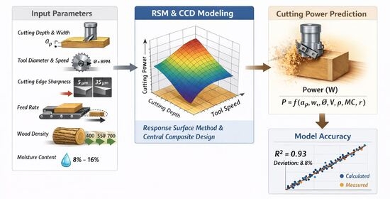
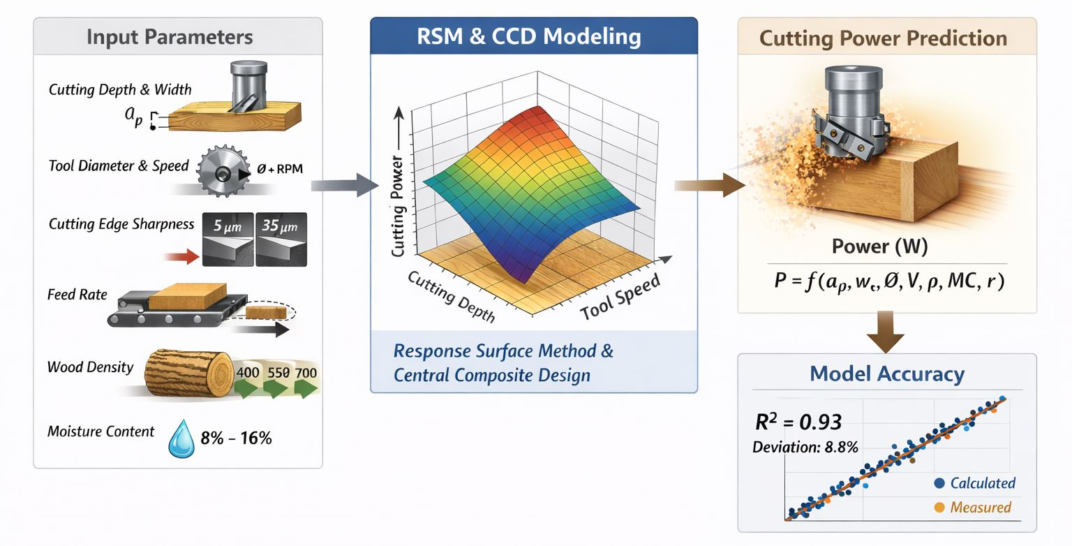
In this study, a model was developed to calculate the power required for the circumferential cutting of solid wood in the longitudinal direction, considering the relevant technological parameters and mechanical properties of the wood. Based on measurements of different combinations and using the Response surface method (RSM) and Central composite design (CCD), a model was created that, in its derived version, considers the cutting width and depth, the diameter and speed of the tool, the number of cutting edges and sharpness of the cutting edge, the feed rate of the workpiece, and the density and moisture content of the wood. The model can be used to calculate the cutting power of various tree species with densities ranging from 400 to 700 kg/m³, moisture contents from 8 to 16%, and a wide range of cutting-edge sharpness, from a sharp cutting edge with a tip radius of 5 µm to a blunt cutting edge with a tip radius of 35 µm. The model is designed for a rake angle of 20°, the value most frequently used in practise. ANOVA analysis was used to determine the suitability of the model, which is highly significant with an R² value of 0.93 and an average deviation of the calculated values from the measured values of 8.8%. The model is robust and therefore useful in the wood industry for predicting energy consumption in the processing of solid wood.

1. Introduction

Energy consumption is an important factor and the general aim is to minimise it. In certain cases, the goal is to optimise energy consumption so that the capacity of a given process is as high as possible for a given energy consumption, while in other cases the goal is to reduce energy consumption for a given capacity. However, minimising energy consumption is not always the most important factor, e.g., if a certain product has to be manufactured to the required quality, even if the energy consumption is higher than it would otherwise be.

Regardless of the situation, it is necessary to know which factors influence energy consumption. With an appropriate model, these factors can be optimised so that energy consumption is optimal in certain cases, or energy consumption can be planned if certain factors are set in order to achieve the desired processing quality [1].

When processing wood, various factors influence the cutting force and therefore the energy consumption. Among the technological factors, the cutting force is influenced by the cutting depth and width, the tool diameter, the number of cutting edges, the rotational speed of the tool, and the feed rate [2,3]. These factors interact in various ways and influence the thickness of the chip and the cutting direction in relation to the grain of the wood, which in turn has a direct effect on the cutting force. In addition, the cutting force is also influenced by the rake angle of the blade [4,5], the sharpness of the blade [6], and the friction between the blade and the wood [7,8], factors over which the production engineer has little or no direct influence. The cutting force decreases as the rake angle increases, but the rake angles in solid wood processing are generally not higher than 20–25° and are on average between 18 and 22°. Longitudinal cutting of solid wood with a rake angle of more than 30° produces a type I chip [9,10], which is characterised by the fact that the tissue is split before the blade tip, i.e., the wood can also be split below the blade tip, resulting in a chipped grain surface, which is undesirable and represents poor machining quality [11]. However, if the rake angle is less than 25° on average, a type II chip is created, which is characterised by the fact that the tissue is not split in front of the tip of the blade, but is created by a combination of pressure and shear failures. In this case, the wood surface is free of chipped grain and represents better surface quality. The rake angle range of 25 to 30° represents a transitional area in which a type I or II chip can occur. With a smaller rake angle of less than 15°, however, the quality of the machined surface can also be worse, as a type III chip can occur, characterised by a combination of pressure failure and tissue splitting in front of the blade tip.

In addition to the technological factors mentioned above, the cutting force, and thus the energy consumption, are also influenced by the density, anatomical characteristics, moisture content [12], and mechanical properties of the wood species in various directions, such as elasticity, strength, and fracture toughness [13]. Various authors have attempted to model cutting force considering various technological and mechanical properties.

Cutting forces have been modelled using the finite element method, taking into account the elasticity, strength, and fracture properties of the material [14,15], as well as cutting models based on strains in the material in front of the tool tip [16]. Various attempts have also been made to create a cutting model that takes into account fracture properties [17,18,19] or is based on different failure criteria and chip breakage due to compressive failure [20,21]. Various models were also created for other orthotropic materials like bone [22,23].

Despite extensive research, there is still no universal model that can be used to calculate cutting forces and power for different combinations of technological parameters and mechanical properties of wood. On the other hand, the existing models are quite challenging for industrial technologists, who need to be familiar with the various mechanical properties of wood, which in certain cases are unknown or hardly available in the generally accessible literature.

An alternative to such models is a mechanistic approach, where the cutting forces are measured based on certain combinations of wood mechanical properties and technological parameters, which can then be used to create a mathematical model that is valid in the tested range on which the model is based. Typically, such models incorporate wood density and moisture content rather than mechanical properties, as there are positive correlations between wood density and its mechanical properties [24].

This approach has been used in numerous studies in which various authors have investigated the effects of different factors on the magnitude of cutting forces or power. Jiang, et al. [25] investigated the effects of rake angle, wedge angle, and clearance angle at different cutting speeds. The influence of chip thickness and tool wear on cutting power was investigated by Pinkowski, et al. [26]. Homkhiew, et al. [27] investigated the influence of cutting speed, workpiece feed, and cutting depth, while Dvoracek, et al. [28] analysed the effects of cutting direction and wood moisture content in linear cutting of oak. Similarly, the influence of blade inclination angle, feed rate, and depth of cut was investigated by Jin and Wei [29] and Li, et al. [30]. A more thorough study of the influence of various technological parameters and wood properties in linear cutting of wood was carried out by Porankiewicz, et al. [31], who created a complex model with more than 50 coefficients. To use the model for circular cutting, the reader has to calculate the average thickness of the chip and determine the average cutting angle between the cutting direction and the tissue orientation. Authors have also used the cutting model for other research. For example, Derbas, et al. [32] used the frequency spectrum in cutting to determine the moisture content of wood or its fracture properties [33].

As already mentioned, an alternative is to use different mathematical models, but to the authors’ knowledge, none of the studies mentioned in the introduction that have been carried out so far fully capture the effects of all relevant technological factors and wood properties and are at the same time simple, robust, and precise. Individual studies have been carried out in which individual authors have created cutting models based on a linear cut under certain conditions. However, these have little practical value in real technological processes, as the user would have to modify the model and calculate the equivalent thicknesses of the chip resulting from the circular cut. On the other hand, various models based on circular cutting contain many numerical constants, which can also lead to a high probability of incorrect calculation of the cutting power, or the models do not contain all relevant technological and material properties.

Given the shortcomings described in the literature regarding existing models, which are either incomplete and do not consider all relevant technological parameters and mechanical properties of wood, or are too complex for industrial use, the purpose of this research is to develop a simple, robust, precise, and comprehensive model for calculating the power required for circular circumferential cutting of solid wood in the longitudinal direction. This model will take into account all relevant technological and material properties of wood and will be suitable for industrial users. The model will be based on the mechanical properties of wood density and moisture content and will include all relevant technological parameters, such as cutting depth and width, workpiece feed, tool speed, tool diameter, and the number and sharpness of cutting knives. Compared to the other models mentioned in the cited articles, this model will be simpler and will include all relevant parameters. The aim of the research is to use the Design of Experiment (DOE) approach [34,35] in the development of the model, which makes it possible to design a robust model with many variables and a relatively small number of experimental combinations, while still considering the main influences of the parameters and their mutual interactions.

Theoretical Background

The basis for the mean cutting force for a single cut can be derived from the relationship between the width b, mean thickness of the chip h_m, and a specific coefficient k_s [36] is

$$F_m=k_s\times b\times h_m$$

(1)

where the specific cutting coefficient k_s depends on the technological parameters and properties of the wood.

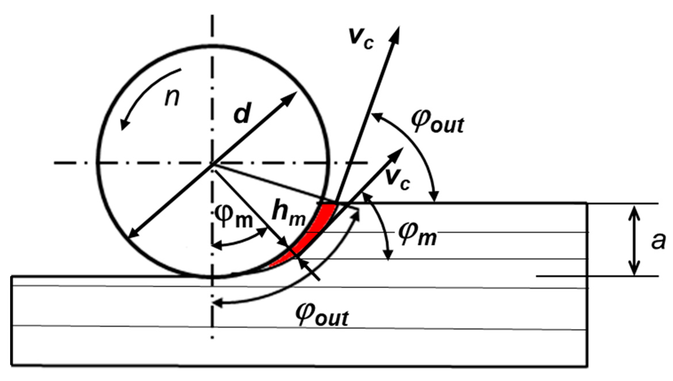
In circular peripheral cutting, the thickness of the chip increases with the angle φ, as shown in Figure 1, which increases the cutting force. When calculating the average cutting force F_m for a single chip, the average chip thickness h_m should be taken into account, which is calculated using the following equation [2]:

$$h_m=f_z\times \sqrt{{\displaystyle \frac{a}{d}}}$$

(2)

Here, a is the depth of cut (Figure 1), d is the diameter of the tool, and f_z is the feed per tooth, which is calculated as follows:

$$f_z={\displaystyle \frac{v_f}{n\times z}}$$

(3)

where v_f is the feed speed and n and z are the rotational speed of the tool and the number of cutting knives, respectively.

In addition to the increase in force due to the increasing chip thickness during circular cutting, the cutting force also increases due to the change in the angle φ between the cutting speed vector v_c and the grain of the wood. For example, the cutting forces are lowest for a longitudinal cut when the angle φ is zero and the velocity vector v_c is parallel to the grain, and highest for a pure cross-section when the angle φ is 90° and the velocity vector is perpendicular to the grain [37].

When calculating the mean cutting force F_m for a single chip during circular cutting, in addition to the changing thickness of the chip, the changing conditions with regard to the cutting direction should also be considered with the corresponding value of the specific cutting force k_s in Equation (1), whereby it is most practical to take into account the values k_s at the mean angle φ_m:

$${\phi }_m={\displaystyle \frac{{\phi }_{out}}{2}}$$

(4)

Here, φ_out is the angle between the blade’s velocity vector and the grain direction at the point where the knife leaves the workpiece (Figure 1), calculated using the equation

$${\phi }_{out}=arccos\left({\displaystyle \frac{r-a}{r}}\right)$$

(5)

where a is the cutting depth and r is the tool radius. If the function is developed into a Taylor series, φ_out can be written in simplified form:

$${\phi }_{out}=2\times \sqrt{{\displaystyle \frac{a}{d}}}$$

(6)

When circular-cutting a thick workpiece with a tool with a large number of cutting knives, there may be a large number of knives in the workpiece at the same time, such as when sawing with a circular saw, where the circular saw blade may have up to 100 or more cutting knives, or there may be only one or even no knife in the workpiece, such as when peripheral-milling or planing workpieces. In this case, the instantaneous cutting force varies from zero, when the knife is not in contact with the wood and is not cutting it, to the maximum force when the knife is cutting and the thickness of the chip is at its greatest. However, the cutting force can also be represented by the average cutting force per chip F_m. If the average cutting power is to be determined, the average cutting force per revolution of the tool should first be determined, which can also be referred to as the operating force F_op and is calculated using the following equation:

$$F_{op}=F_m\times z_{ef}$$

(7)

F_m is the mean force per chip, and z_ef is the average number of cutting knives. For example, z_ef can be between 0 and 1 when circumferential milling or planing with tools with a smaller number of cutting knives, where no knife or only one knife cuts at a time, and is calculated using the following equation:

$$z_{ef}={\displaystyle \frac{z\times {\widehat{\phi }}_{out}}{2\pi }}={\displaystyle \frac{z\times 2\times \sqrt{\frac{a}{d}}}{2\pi }}={\displaystyle \frac{z}{\pi }}\times \sqrt{{\displaystyle \frac{a}{d}}}$$

(8)

With the F_op, the torque M_c and cutting power P_c can be calculated as follows:

$$M_c=F_{op}\times {\displaystyle \frac{d}{2}}$$

(9)

$$P_c=M_c\times \omega$$

(10)

where ω is the angular speed in rad/s.

The basis of the mechanistic approach is therefore the specific cutting force coefficient k_s in Equation (1), which considers various technological parameters, as well as the mechanical properties of the wood. In the past, several studies [38] were carried out in which the authors presented the effects of the various factors in the form of tables and diagrams. The user then had to read the individual coefficients from the diagrams based on specific factors and combine them into a general coefficient k_s. This approach is quite time-consuming and unreliable, as the user can easily make mistakes in their calculations.

2. Materials and Methods

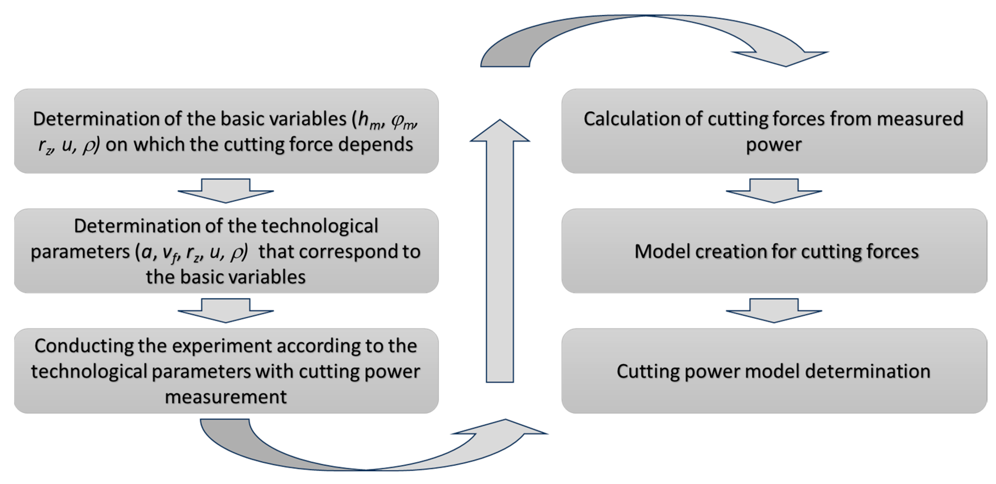
As described, the average cutting force F_m for a chip depends directly on the thickness of the chip h_m, the cutting angle relative to the grain φ_m, the sharpness of the knife r_z, the moisture content of the wood u, and the density of the wood ρ. Once the cutting force F_m has been determined, the cutting power can be further determined using Equations (7)–(10). It is therefore important to first determine the influence of the basic factors on the size of the cutting force. The test procedure is shown in Figure 2. Firstly, the basic parameters on which the model for determining the cutting forces is based are determined. Then, the corresponding technological parameters for carrying out the test are determined, whereby the values of the basic parameters correspond to the required parameters. A cutting test is carried out with the technological parameters determined, and the cutting power is measured. The average force F_m per chip is then calculated from the measured power and used to create a model to determine the cutting forces, which in turn is used to create a model to calculate cutting power.

2.1. Material Preparation

Three tree species with different densities were used in the experiment: spruce (Picea abies (L.) Karst), lime (Tilia platyphyllos Scop.), and beech (Fagus sylvatica L.), such that the difference between the average density of the first and second species and the second and third species was the same. First, samples measuring 750 mm × 100 mm × 30 mm were prepared from boards of different dimensions, which were then equilibrated at standard air conditions of 22 °C and 65% relative humidity. After equilibration, the density of the samples was determined, and then the density of the absolutely dry wood was calculated. On this basis, the samples were sorted so that their average density was 662.2 kg/m³ for beech, 537.1 kg/m³ for lime, and 404.8 kg/m³ for spruce, with standard deviations (SDs) of 13.7 kg/m³, 10.7 kg/m³, and 10.5 kg/m³ and coefficients of variation (COVs) of 2.07%, 1.99%, and 5.06%, respectively. All samples were selected so that the lateral surface that was cut had a radial texture, so that the same amount of earlywood and latewood was cut in each cut. In this way, the influence of the different densities of earlywood and latewood was eliminated. The samples of each tree species were divided into three groups, with one group equilibrated at a relative humidity of 88%, the second group at 67%, and the third group at 44%. The equilibrium moisture content (EMC) of wood was determined gravimetrically by weighing moist and absolutely dry samples, and the EMC was calculated from the difference in mass relative to the weight of the dry samples. When the samples reached the desired EMC (22 °C), which averaged 8.1%, 11.9%, and 16.2% for all species, they were sawn to the final dimensions of 750 mm × 100 mm × 26 mm.

2.2. Cutting Experiment

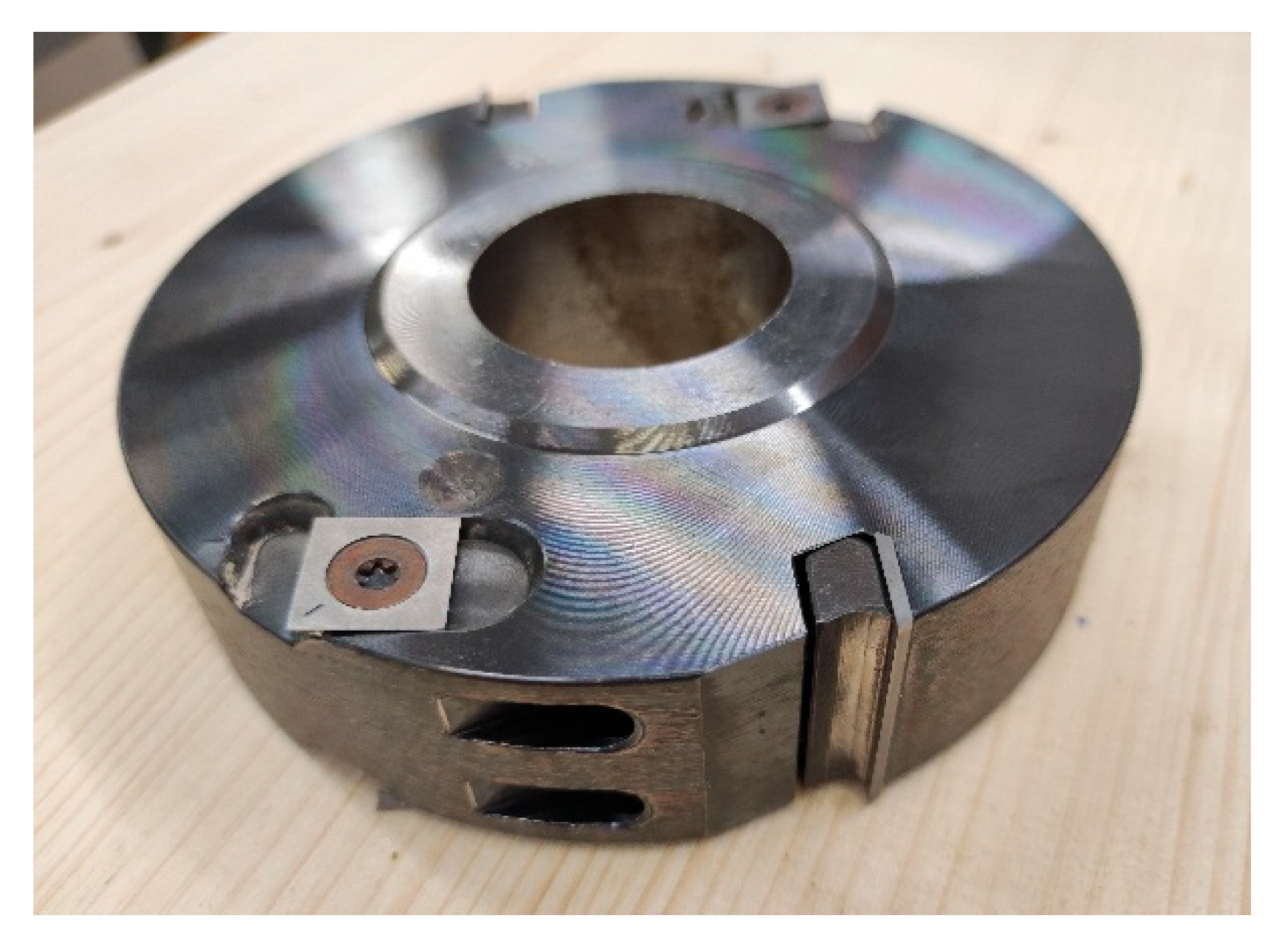
The cutting experiment was performed on an SCM T130 (SCM, Rimini, Italy) spindle moulder with a feed device Maggi STEFF 2048 (Maggi, Certaldo, Italy) connected to a Frenic 5000G11 (Fuji Electric, Edison, NJ, USA) frequency converter, which allowed the desired feed speeds to be set. A 125 mm diameter cutterhead (Figure 3) with two turnblade knives and a 20° rake angle was used, and the speed was 6000 rpm. As the tool clamp did not have a jointing system that allowed both knives to be set to the same cutting diameter, the experiment was carried out so that only one knife cut, while the cutting edge of the other knife was ground so that the cutting diameter of the second knife was 1 mm smaller than the diameter of the knife that was cutting. Replaceable tungsten carbide cutting inserts measuring 30 mm × 12 mm × 1.5 mm and with a wedge angle of 60° were used in the experiment. Three cutting edge sharpnesses were used. The different sharpenings were achieved by first milling 30 mm thick oak samples with the knife in such a way that the cutting edge was worn down evenly. During the wear process, the radius of the cutting edge was measured using a LEXT OL5000 3D (Olympus, Westborough, MA, USA) laser scanning microscope, taking 30 measurements along the cutting edge and calculating the average radius value. In the experiment, the knives therefore had average cutting-edge rounding radii of 5.2 µm, 19.1 µm, and 34.9 µm, with standard deviations of 1.1 µm, 3.1 µm, and 3.1 µm, respectively. As the rake angles in the industry for milling solid wood in longitudinal direction are on average between 18° and 22°, only a rake angle of 20° was used in the experiment, as no significant differences would be recognizable with a smaller rake angle of 18° or a larger one of 22°.

2.3. Planning the Experiment

The Design of Experiments (DOE) method using Design Expert software (Stat-Ease, Minneapolis, MN, USA, v13), Response Surface Modelling (RSM), and Central Composite Design (CCD) was used to plan the experiment and matrix. The CCD method is particularly useful if you want to build a second-order quadratic modelling system, as it allows you to efficiently determine main effects, interactions, and curvatures without having to perform a full three-stage factorial experiment, which can be very extensive, with a large number of variables [39,40].

In the experiment, a full factorial rotatable design with the basic part of the 2^k plan with n_k number of factorial points is used with a standard two-level factorial design at low “−1” and high “+1” levels to determine main effects and interactions. Additional symmetrically arranged axial points n_α are added along each axis at a distance of ±α around the centre of the plan to capture the curvature of the response. In our case, the experimental design was face-centred with α = 1. To perform a dispersion analysis of experimental or model results (calculating the error, testing the significance of model coefficients, checking the adequacy and determining the confidence limits of the model, determining the curvature, etc.), the model requires a certain number n₀ of runs at the central values of the variation factors. The use of the system of n₀ runs at the central point is only justified under the assumption that the errors are the same for each run in the covered multifactor space. Normally, the number of central points is four to six, but in this experiment, due to wood variability, eight repetitions were performed at the central point of the plan (n₀ = 8) at the central values of the variation factors.

In general form, the number of experiments is obtained from the equation

$$N=2^k+2k+n_0=n_k+n_{\alpha }+n_0$$

(11)

where N is the total of experiments or combinations, k is the number of parameters, n_k (n_k = 2^k) is the number of factorial points, n_α (n_α = 2k) is the number of symmetrically placed points around the centre of the plan, and n₀ is the number of repetitions at the centre point of the plan.

In the experiment, five factors were included (k = 5), so the total number of experiments is

$$N=32+10+8=50$$

(12)

In the experiment, the average angle φ_m between the cutting vector and the tissue varied at different cutting depths a, so the calculation of the appropriate depth was performed according to Equations (4) and (5). However, as the mean thickness of the chip h_m increased with increasing depth of cutting, the feed rate also needed to be adjusted to ensure that the mean thickness of the chip met the required conditions. The corresponding feed rate was therefore calculated using Equations (2) and (3).

Five variables with three different values were included in the experiment, whereby the minimum and maximum values were taken from the most common process parameters. Their values are listed in

Table 1. Real value parameters and parameters used in DOE cutting model.

	Real Values
	Min	Mean	Max
Mean chip thickness, hm (mm)	0.1	0.25	0.4
Mean cutting angle, φm (°)	5	15	25
Tool tip radius, rz (µm)	5.2	19.1	34.9
Wood moisture content, u (%)	8.1	11.9	16.2
Wood density, ρ (kg/m3)	404.8	537.1	662.2
	Modelled values
	−1	0	1
Mean chip thickness, hm (m)	0.0001	0.0003	0.0004
Mean cutting angle, φm (rad)	0.087	0.262	0.436
Tool tip radius, rz (µm)	5	20	35
Wood moisture content, u (%)	8	12	16
Wood density, ρ (kg/m3)	405	535	665

.

As it is important for the CCD model used in the experiment that the differences in the values of the individual variables between the minimum and average values and between the average and maximum values are the same, the values given in the lower part of Table 1 were considered in the model. The values used for model differ slightly from the actual values, but the differences are minimal, and the values have been converted to base units so that the resulting model can be manipulated more easily.

The experiment combinations with coded, modelled, and corresponding technological factors are shown in

Table A1. Coded and modelled factors, together with corresponding technological factors.

	Coded Factors					Modelled Factors					Corresponding Technological Factors
	Density	Humidity	Chip Thickness	Cutting Edge radius	Mean Cutting Angle	Density	Humidity	Chip Thickness	Cutting Edge Radius	Mean Cutting Angle	Density	Humidity	Feed Rate	Cutting Edge Radius	Cutting Depth
STD	ρ	u	hm	rz	φm	ρ (kg/m3)	u (%)	hm (m)	rz (µm)	φm (rad)	ρ (kg/m3)	u (%)	vf (m/min)	rz (µm)	a (mm)
1	−1	−1	−1	−1	−1	405	8	0.0001	5	0.0873	405	8	13.8	5	0.95
2	1	−1	−1	−1	−1	665	8	0.0001	5	0.0873	665	8	13.8	5	0.95
3	−1	1	−1	−1	−1	405	16	0.0001	5	0.0873	405	16	13.8	5	0.95
4	1	1	−1	−1	−1	665	16	0.0001	5	0.0873	665	16	13.8	5	0.95
5	−1	−1	1	−1	−1	405	8	0.0004	5	0.0873	405	8	55.0	5	0.95
6	1	−1	1	−1	−1	665	8	0.0004	5	0.0873	665	8	55.0	5	0.95
7	−1	1	1	−1	−1	405	16	0.0004	5	0.0873	405	16	55.0	5	0.95
8	1	1	1	−1	−1	665	16	0.0004	5	0.0873	665	16	55.0	5	0.95
9	−1	−1	−1	1	−1	405	8	0.0001	35	0.0873	405	8	13.8	35	0.95
10	1	−1	−1	1	−1	665	8	0.0001	35	0.0873	665	8	13.8	35	0.95
11	−1	1	−1	1	−1	405	16	0.0001	35	0.0873	405	16	13.8	35	0.95
12	1	1	−1	1	−1	665	16	0.0001	35	0.0873	665	16	13.8	35	0.95
13	−1	−1	1	1	−1	405	8	0.0004	35	0.0873	405	8	55.0	35	0.95
14	1	−1	1	1	−1	665	8	0.0004	35	0.0873	665	8	55.0	35	0.95
15	−1	1	1	1	−1	405	16	0.0004	35	0.0873	405	16	55.0	35	0.95
16	1	1	1	1	−1	665	16	0.0004	35	0.0873	665	16	55.0	35	0.95
17	−1	−1	−1	−1	1	405	8	0.0001	5	0.4364	405	8	2.8	5	22.33
18	1	−1	−1	−1	1	665	8	0.0001	5	0.4364	665	8	2.8	5	22.33
19	−1	1	−1	−1	1	405	16	0.0001	5	0.4364	405	16	2.8	5	22.33
20	1	1	−1	−1	1	665	16	0.0001	5	0.4364	665	16	2.8	5	22.33
21	−1	−1	1	−1	1	405	8	0.0004	5	0.4364	405	8	11.2	5	22.33
22	1	−1	1	−1	1	665	8	0.0004	5	0.4364	665	8	11.2	5	22.33
23	−1	1	1	−1	1	405	16	0.0004	5	0.4364	405	16	11.2	5	22.33
24	1	1	1	−1	1	665	16	0.0004	5	0.4364	665	16	11.2	5	22.33
25	−1	−1	−1	1	1	405	8	0.0001	35	0.4364	405	8	2.8	35	22.33
26	1	−1	−1	1	1	665	8	0.0001	35	0.4364	665	8	2.8	35	22.33
27	−1	1	−1	1	1	405	16	0.0001	35	0.4364	405	16	2.8	35	22.33
28	1	1	−1	1	1	665	16	0.0001	35	0.4364	665	16	2.8	35	22.33
29	−1	−1	1	1	1	405	8	0.0004	35	0.4364	405	8	11.2	35	22.33
30	1	−1	1	1	1	665	8	0.0004	35	0.4364	665	8	11.2	35	22.33
31	−1	1	1	1	1	405	16	0.0004	35	0.4364	405	16	11.2	35	22.33
32	1	1	1	1	1	665	16	0.0004	35	0.4364	665	16	11.2	35	22.33
33	−1	0	0	0	0	405	12	0.00025	20	0.2617	405	12	11.5	20	8.37
34	1	0	0	0	0	665	12	0.00025	20	0.2617	665	12	11.5	20	8.37
35	0	−1	0	0	0	535	8	0.00025	20	0.2617	535	8	11.5	20	8.37
36	0	1	0	0	0	535	16	0.00025	20	0.2617	535	16	11.5	20	8.37
37	0	0	−1	0	0	535	12	0.0001	20	0.2617	535	12	4.6	20	8.37
38	0	0	1	0	0	535	12	0.0004	20	0.2617	535	12	18.4	20	8.37
39	0	0	0	−1	0	535	12	0.00025	5	0.2617	535	12	11.5	5	8.37
40	0	0	0	1	0	535	12	0.00025	35	0.2617	535	12	11.5	35	8.37
41	0	0	0	0	−1	535	12	0.00025	20	0.0873	535	12	34.4	20	0.95
42	0	0	0	0	1	535	12	0.00025	20	0.4364	535	12	7.0	20	22.33
43	0	0	0	0	0	535	12	0.00025	20	0.2617	535	12	11.5	20	8.37
44	0	0	0	0	0	535	12	0.00025	20	0.2617	535	12	11.5	20	8.37
45	0	0	0	0	0	535	12	0.00025	20	0.2617	535	12	11.5	20	8.37
46	0	0	0	0	0	535	12	0.00025	20	0.2617	535	12	11.5	20	8.37
47	0	0	0	0	0	535	12	0.00025	20	0.2617	535	12	11.5	20	8.37
48	0	0	0	0	0	535	12	0.00025	20	0.2617	535	12	11.5	20	8.37
49	0	0	0	0	0	535	12	0.00025	20	0.2617	535	12	11.5	20	8.37
50	0	0	0	0	0	535	12	0.00025	20	0.2617	535	12	11.5	20	8.37

in Appendix A.

2.4. Power Measurements

With the combinations obtained in this way, an experiment was carried out in which three repetitions were performed for each combination. For each repetition, the cutting power was calculated by first measuring the power at idle and then measuring the power during cutting and using the difference to calculate the cutting power.

The power was calculated by measuring the voltage (U) and current (I) on all three phases of the electric motor driving the table cutter. An electrical voltage transformer was used to convert the electrical voltage from the −400 to +400 V range to the −10 to +10 V range, and an electrical current transformer was used to generate a voltage proportional to the current, also in the −10 to +10 V range. All voltages were acquired using a National Instruments NI-USB 6351 (National Instruments, Austin, TX, USA) acquisition card with a sampling frequency of 2500 Hz and then converted to the real voltage and current values. National Instruments LabVIEW (National Instruments, Austin, TX, USA, v2023) software was used for acquisition and calculation. The power for each phase was calculated 10 times per second, using 250 samples of U and I for each calculation, by multiplying the instantaneous values of voltage and current for each phase separately. The total power was the sum of the power from all three phases [2].

The cutting power was determined as an average value over the entire length of the workpiece and used to calculate the cutting forces. First, M_c from Equation (10) and then F_op and F_m from Equations (7) and (9) were determined. The mean force per chip F_m was then normalised to a cutting width of 1 m, so that the values were divided by the segment width of 0.026 m. The normalised values F_mb were then entered into the Design Expert software (v 13), where a detailed ANOVA analysis was performed to determine the significance of the individual parameters and their interactions, and a suitable mathematical model for F_mb was created. The model obtained for F_mb was then converted into a model for calculating the cutting power P_c using Equations (1)–(10), considering the technological parameters and the density and moisture content of the wood in the manner shown in Figure 2.

3. Results and Discussion

The power measurements, together with the average values and coefficients of variation (COVs) for individual combinations, where three repetitions were performed for each combination, are shown in

Table 2. Measured power values and corresponding forces.

	Response 1	Response 2	Response 3	Average Value	Coefficient of Variation (Power)	Mean Force Per Chip	Normalised Mean Force Per Chip
	P1	P2	P3	P	COV	Fm	Fmb
STD	(W)	(W)	(W)	(W)	(%)	(N)	(N/m)
1	79	83	75	79	4.13	73	2807
2	120	124	103	116	7.87	107	4111
3	127	113	103	114	8.61	106	4064
4	135	118	144	132	8.15	122	4706
5	213	181	181	192	7.87	177	6824
6	255	278	313	282	8.46	261	10,045
7	196	222	243	220	8.72	204	7859
8	309	269	283	287	5.77	266	10,238
9	96	113	117	109	8.38	100	3864
10	180	179	136	165	12.43	153	5871
11	126	168	148	147	11.64	136	5242
12	162	175	193	177	7.19	163	6287
13	236	213	218	222	4.44	206	7919
14	293	331	387	337	11.46	312	12,010
15	249	287	239	258	8.00	239	9178
16	313	305	290	303	3.15	280	10,772
17	578	624	671	624	6.08	116	4453
18	858	749	815	807	5.55	150	5762
19	616	604	677	632	5.05	117	4511
20	972	972	864	936	5.44	174	6687
21	1199	1138	1257	1198	4.06	223	8569
22	1509	2082	2492	2028	19.88	378	14,557
23	1323	1390	1487	1400	4.81	260	10,017
24	2726	2685	2844	2752	2.45	515	19,825
25	849	1012	1002	954	7.82	177	6815
26	1141	1091	1195	1142	3.72	212	8158
27	1145	874	871	963	13.34	179	6875
28	1343	1342	1350	1345	0.26	250	9618
29	1434	1782	1245	1487	14.96	277	10,651
30	2008	1633	2055	1899	9.95	354	13,627
31	2327	1773	2086	2062	11.00	385	14,813
32	2550	3121	2675	2782	8.81	521	20,023
33	610	678	479	589	14.02	182	7000
34	756	856	986	866	10.87	268	10,310
35	656	772	709	712	6.66	220	8477
36	919	988	886	931	4.56	288	11,083
37	651	650	619	640	2.32	198	7614
38	972	894	1232	1033	13.99	320	12,305
39	626	633	676	645	3.43	199	7673
40	1020	823	828	890	10.30	276	10,596
41	224	238	257	240	5.64	222	8534
42	1603	1668	1648	1640	1.66	306	11,759
43	890	877	837	868	2.60	269	10,335
44	757	805	1019	860	13.24	266	10,248
45	833	885	908	875	3.58	271	10,422
46	1040	802	809	884	12.51	274	10,526
47	894	923	826	881	4.61	273	10,492
48	841	774	1045	887	13.00	274	10,557
49	843	930	882	885	4.02	274	10,537
50	1035	743	863	880	13.61	272	10,473

. Individual COV values for all combinations range from 0.26% to 19.88%, with an average COV value of 7.80%. For combinations with standard order (STD) 43 to 50, which belong to group n₀ for the dispersion analysis, and are made at the centre point of the plan, the average power value is 877.5 W, the standard deviation is 85.03 W, and the COV is 9.69%. Although the COV values for cutting power are higher than the COV values for wood density, where they averaged 3.04%, they can still be considered low values, as in general the variability of the mechanical properties of wood at the same density can be quite high [24]. The analysis also confirms the fact that a threefold repetition for each combination is sufficient, as the differences between individual measurements are relatively small. The reason for the low COV values can also be attributed to the fact that the surface that was cut had a strictly radial surface, where the amount of earlywood and latewood was always the same during cutting. When cutting a surface with a tangential texture, the differences in power would be much greater for the same combination, as one cut could be mainly earlywood, another mainly latewood, and a third a combination of earlywood and latewood. In this case, it would be necessary to perform a larger number of repetitions for the same combination of parameters to obtain a representative average value, as is the case when cutting a surface with radial texture. Table 2 also shows the average power values, the mean forces per chip F_m calculated with Equations (7)–(10) for a chip with a cutting width of 26 mm, and the normalised force values F_mb for a cutting width of 1 m, which were further used in the model development and the detailed statistical analysis.

The results of the ANOVA analysis are shown in

Table 3. Fit summary for various models (2FI—2 factor interaction).

Source	Sequential p-Value	Lack of Fit p-Value	Adjusted R2	Predicted R2
Linear	<0.0001	<0.0001	0.8076	0.7637
2FI	0.0057	<0.0001	0.8711	0.7584
Quadratic	0.0042	<0.0001	0.9140	0.8085	Suggested
Cubic	0.0032	<0.0001	0.9702	0.3511	Aliased

. The analysis shows that the quadratic equation fits best, as it has the highest R² and is also suggested by Design Expert. However, for further analysis, the reduced quadratic equation is used, as the use of the quadratic equation can lead to problems when the model is applied outside the tested range, where the positive trend can become negative due to the nature of the quadratic equation. According to studies by cited authors who have investigated the effects of individual parameters, the force increases for all parameters except moisture, where the force initially increases up to a wood moisture content of around 12% and then begins to decrease at higher moisture contents. To obtain a positive trend for all parameters except moisture content, the quadratic terms for all variables except moisture content were removed from the equation so that the model could show an initial increase in force and then a decrease with increasing wood moisture content.

The ANOVA results of the reduced quadratic equation are shown in

Table 4. ANOVA analysis for the reduced quadratic model.

Source	Sum of Squares	df	Mean Square	F-Value	p-Value
Model	5.92 × 108	16	3.70 × 107	30.82	<0.0001
A–ρ	7.69 × 107	1	7.69 × 107	64.04	<0.0001
B–u	2.19 × 107	1	2.19 × 107	18.22	0.0002
C–hm	3.05 × 108	1	3.05 × 108	253.64	<0.0001
D–r	2.58 × 107	1	2.58 × 107	21.47	<0.0001
E–φm	9.35 × 107	1	9.35 × 107	77.85	<0.0001
AB	3.52 × 105	1	3.52 × 105	0.29	0.5918
AC	1.61 × 107	1	1.61 × 107	13.40	0.0009
AD	1.06 × 106	1	1.06 × 106	0.88	0.3549
AE	7.29 × 106	1	7.29 × 106	6.07	0.0192
BC	4.79 × 106	1	4.79 × 106	3.98	0.0543
BD	3.03 × 105	1	3.03 × 105	0.25	0.6189
BE	6.92 × 106	1	6.92 × 106	5.76	0.0222
CD	6.53 × 105	1	6.53 × 105	0.54	0.4663
CE	1.42 × 107	1	1.42 × 107	11.81	0.0016
DE	1.02 × 106	1	1.02 × 106	0.84	0.3637
B2	1.69 × 107	1	1.69 × 107	14.06	0.0007

. The Model F-value of 30.82 implies that the model is significant. There is only a 0.01% chance that an F-value this large could occur due to noise.

p-values less than 0.05 indicate that the model terms are significant. In this case, A, B, C, D, E, AC, AE, BC, BE, CE, and B² are significant model terms. Values greater than 0.10 indicate that the model terms are not significant, and these terms were removed from the model to simplify it.

The resulting model for calculating the F_mb for coded and actual factors is shown in

Table 5. Coefficients in terms of coded and actual factors.

Coded Factors		Actual Factors
Fmb	=	Fmb	=
+9961.31		–4986.22
+1504.25	A–ρ	–3.03	ρ
+802.31	B–u	+1733.99	u
+2993.67	C–hm	–1.389 × 107	hm
+870.91	D–rz	+58.06	rz
+1658.50	E–φm	–16,104.52	φm
+709.27	AC	+36,372.87	ρ × hm
+477.19	AE	+21.03	ρ × φm
+386.71	BC	+6.44 × 105	u × hm
+465.17	BE	+666.32	u × φm
+665.93	CE	+2.54 × 107	hm × φm
−1245.99	B2	−77.87	u2

. In the case of coded factors, the coded values of the variables, i.e., −1, 0, and 1, should be used for the calculation. The advantage of coded factors is that they show the relative importance of individual variables or combinations of variables. For example, it can be deduced from the coded factors that the thickness of the chip h_m, whose coded factor has the highest value, has the greatest influence on the cutting forces, followed by the φ_m, ρ, r_z, and u. The model is also influenced by the interaction of various variables with approximately equal effects.

Table 6. Fit statistics.

R2	Adjusted R2	Predicted R2	Adeq Precision	Std. Dev.	Mean	C.V. %
0.93	0.91	0.87	30.23	1064.11	9114.03	11.68

shows the model fit statistics, where R², Adjusted R², and Predicted R² are 0.93, 0.91, and 0.87, respectively. The Predicted R² of 0.87 is in reasonable agreement with the Adjusted R² of 0.91, where the difference is less than 0.2. Also, Adeq Precision, which should be greater than 4 and measures the signal-to-noise ratio, is 30.22, which indicates an adequate signal and suggests that the model can be used to navigate the design space, while the coefficient of variation is 11.68%, which is also acceptable.

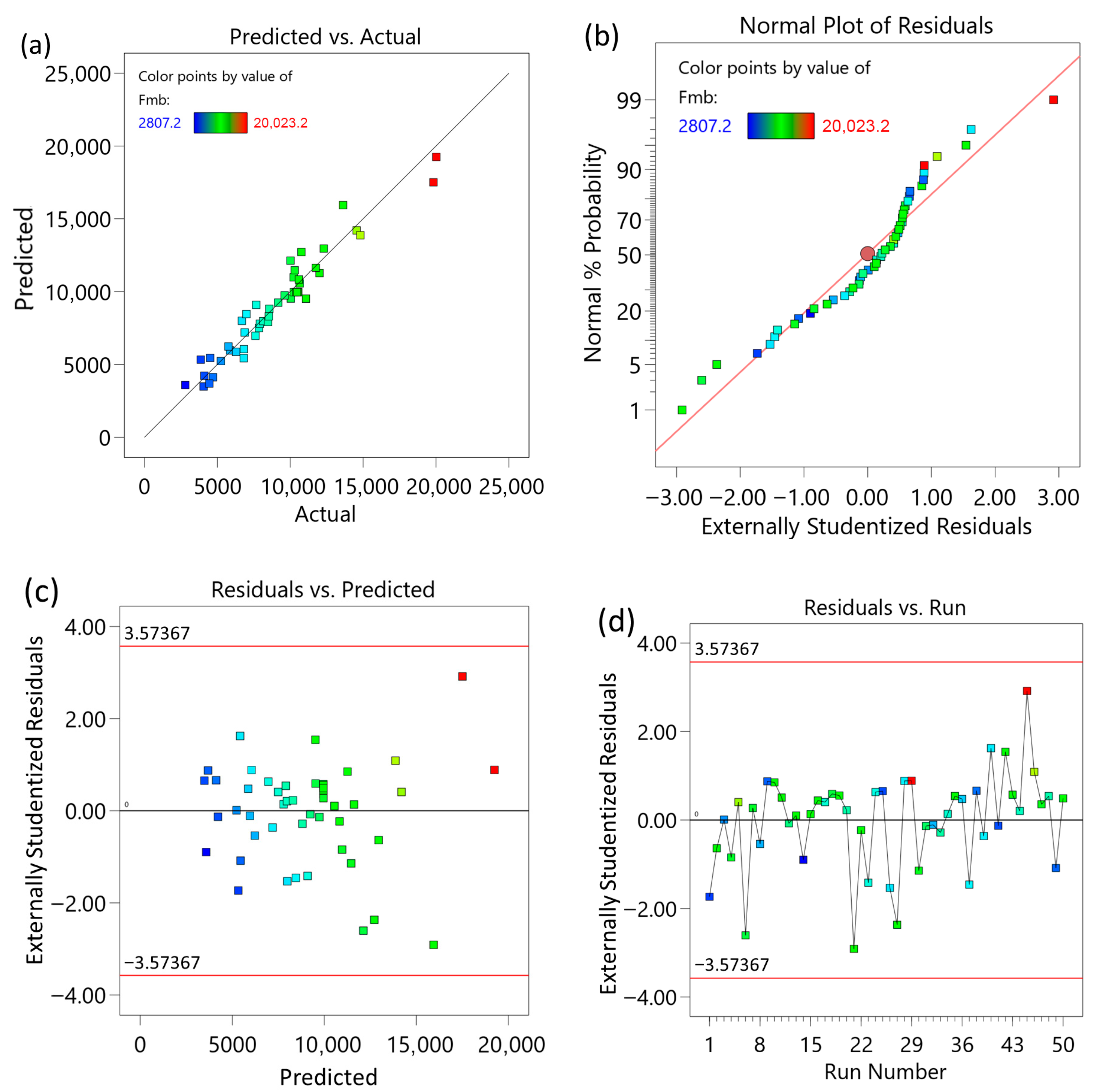
The relationship between the measured and calculated F_mb is shown in Figure 4a. The linear trend between them is obvious and confirms the suitability of the model for calculating the cutting forces, which is also confirmed by the normal curve of the residuals (Figure 4b), which also runs around the straight line. Figure 4c shows that the values are within the residual limits and have a random distribution, while Figure 4d shows that the residuals do not depend on the number of runs.

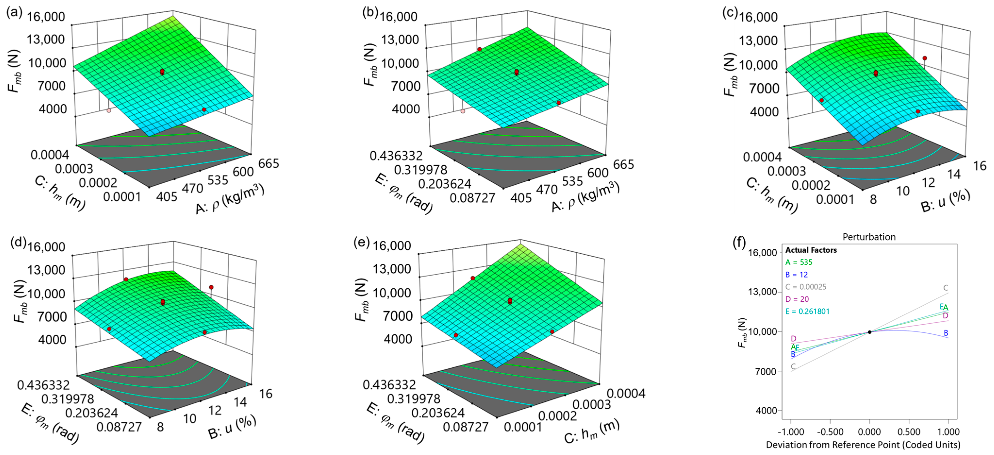
The effects of the various factors and their interactions are shown in Figure 5. The trend of a particular factor depends on the value of another factor with which the first factor interacts. F_mb increases faster with increasing h_m at higher ρ than at lower ρ (Figure 5a). The same is true for the increase in F_mb with a change in φ_m, with F_mb also increasing faster at a higher ρ than at a lower ρ (Figure 5b). The effect of moisture content on the F_mb can be seen in Figure 5c, where F_mb increases faster with h_m in moist wood than in dry wood, and the F_mb also increases faster with φ_m in moist wood than in dry wood (Figure 5d). Looking at moisture content, F_mb initially increases with u up to a certain value and then starts to decrease as u increases further (Figure 5d), which is also consistent with the trend of other mechanical properties [41] that initially increase up to a certain moisture content and then decrease as the moisture content of the wood increases. There is also an interaction between φ_m and h_m (Figure 5e), with F_mb increasing faster with h_m in a more transverse cut (bigger φ_m) than in a longitudinal cut (smaller φ_m). The perturbation plot in coded values, which shows how the response changes as each factor moves away from the chosen reference point while all other factors are held constant at the reference value in the centre of the design space, is shown in Figure 5f. The figure clearly shows that factor C has the largest slope and therefore the largest influence on the increase in F_mb, followed by factors E, A, D, and B, as already shown in Table 5.

To obtain the model for calculating the cutting power with actual technological parameters, the equation on the right-hand side of Table 5 should be considered. Then, the equation should be multiplied by the cutting width (b), and then Equations (2) and (3) for h_m and Equations (4) and (6) for φ_m should be used. In addition, the resulting equation should be multiplied by the average number of knives (z_ef) cutting per unit time (Equation (7)), the tool diameter (d), and the angular velocity (ω) using Equations (9) and (10). After rearranging the equation so that practical units can be used, the final model for calculating the power of peripheral cutting of solid wood in a longitudinal direction with a knife having a rake angle of 20° (or approximately 20°) can be written as follows:

$$\begin{array}{cc}Pc=b\left[a\right(nz(\hfill & -0.000268+0.0000111u+3.5\times {10}^{-7}\rho )+v_f(-0.231\hfill \\ & +0.4239\sqrt{{\displaystyle \frac{a}{d}}}+0.01074u+0.000606\rho ))\hfill \\ & +nz\sqrt{ad}(-0.0000831+9.676\times {10}^{-7}{r}_z+0.0000288u\hfill \\ & -0.000001297u^2-5.047\times {10}^{-8}\rho )]\hfill \end{array}$$

(13)

where b is the cutting width in mm, a is the cutting depth in mm, d is the tool diameter in mm, n is the tool rotational speed in rpm, z is the number of tool knifes, v_f is the feed speed in m/min, r_z is the blade sharpness radius in µm, u is the wood moisture content in %, and ρ is the wood density in kg/m³.

The verification of the model is shown in

Table 7. Actual and predicted values of cutting power and their differences.

	Actual Values-P	Predicted Values-Pc	Difference		Actual Values-P	Predicted Values-Pc	Difference
STD	(W)	(W)	(%)	STD	(W)	(W)	(%)
1	79.0	101.8	28.9	26	1142.3	1131.2	1.0
2	115.7	119.9	3.6	27	963.3	1020.2	5.9
3	114.3	99.0	13.4	28	1345.0	1381.1	2.7
4	132.3	117.1	11.5	29	1487.0	1497.6	0.7
5	191.7	171.7	10.4	30	1898.7	2260.8	19.1
6	282.0	270.2	4.2	31	2062.0	1966.8	4.6
7	220.3	212.8	3.4	32	2782.0	2730.0	1.9
8	287.0	311.3	8.5	33	589.0	719.4	22.1
9	108.7	151.3	39.2	34	866.0	975.3	12.6
10	165.0	169.3	2.6	35	712.3	673.1	5.5
11	147.3	148.4	0.8	36	931.0	809.6	13.0
12	176.7	166.5	5.8	37	640.0	592.7	7.4
13	222.3	221.1	0.5	38	1032.7	1102.0	6.7
14	337.0	319.7	5.1	39	645.0	773.3	19.9
15	258.3	262.2	1.5	40	890.3	921.5	3.5
16	302.7	360.7	19.2	41	239.7	235.5	1.7
17	624.3	523.4	16.2	42	1639.7	1647.9	0.5
18	807.3	884.2	9.5	43	868.0	847.4	2.4
19	632.3	773.2	22.3	44	860.3	847.4	1.5
20	936.0	1134.0	21.2	45	875.3	847.4	3.2
21	1198.0	1250.5	4.4	46	883.7	847.4	4.1
22	2027.7	2013.7	0.7	47	881.0	847.4	3.8
23	1400.0	1719.7	22.8	48	886.7	847.4	4.4
24	2751.7	2482.9	9.8	49	885.0	847.4	4.3
25	954.3	770.4	19.3	50	880.3	847.4	3.7

, which shows the power calculations based on the model (Equation (13)) and the measured values. The difference between the calculated and measured values is on average 8.8%, which is a relatively small deviation, especially considering the relatively high variability of density within tree species and, at the same density, the variability of mechanical properties [24] that actually affect the force, and thus the cutting power [11].

4. Conclusions

In this study, a model was developed to calculate the power required for circular cutting of solid wood in the longitudinal direction. The experiment was designed and conducted with five input parameters, which were varied at three levels. The model is essentially based on the thickness of the chip, the cutting angle between the speed vector of the knives and the orientation of the wood tissue, the sharpness of the knives, and the density and moisture content of the wood. Using geometric and kinematic relationships, a model is then derived that contains the following actual technological parameters: cutting width and depth, tool diameter and speed, number and sharpness of the knives as well as feed rate, and density and moisture content of the workpiece.

The developed model can be used to calculate the cutting power for various tree species with densities ranging from 400 kg/m³ to 700 kg/m³, moisture contents from 8% to 16%, and a wide range of cutting edge sharpnesses, from a sharp cutting edge with a tip radius of 5 µm to a blunt cutting edge with a tip radius of 35 µm. The model is based on a rake angle of 20°, which on average is the most commonly used angle for machining solid wood in the longitudinal direction and is therefore not suitable for knives with significantly smaller or larger rake angles.

Detailed statistical analysis of the test results and a comparative analysis of the modelled and experimental cutting force values confirmed that the derived model is highly significant, with all parameters in the model being significant. The developed model is simple and robust and allows calculation of the cutting power with an average accuracy of 8.8%, which is a relatively high accuracy, especially considering the high variability of mechanical properties for a given tree species or wood density.

The model represents a significant contribution, as, to the authors’ knowledge, there is currently no such comprehensive, robust, and simple model available in the literature that considers all important technological parameters, as well as basic wood properties such as wood density and moisture content.

The model can be used for both research and industrial purposes for advanced calculation of cutting power, allowing planning of production and economic aspects of the process, as it enables calculation of energy consumption for a specific operation.

However, the model that was developed can only be used for peripheral cutting of solid wood in the longitudinal direction and is not suitable for composite materials or for cutting solid wood in the perpendicular direction. In the first case, the mechanical properties can be very different from those of solid wood, and in the second case, the properties of solid wood in the transverse direction are different from those in the longitudinal direction.

References

1. Chavenetidou, M.; Kamperidou, V. Impact of Wood Structure Variability on the Surface Roughness of Chestnut Wood. Appl. Sci. 2024, 14, 6326. [Google Scholar] [CrossRef] [Scilit]
2. Merhar, M.; Bjelić, A.; Hodžić, A. Modelling of Peripheral Wood Milling Power Using Design of Experiment Approach. Drv. Ind. 2024, 75, 395–404. [Google Scholar] [CrossRef] [Scilit]
3. Wellenreiter, P.; Hernández, R.E.; Cáceres, C.B.; Blais, C. Cutting forces and noise in helical planing black spruce wood as affected by the helix angle and feed per knife. Wood Mater. Sci. Eng. 2023, 18, 549–558. [Google Scholar] [CrossRef] [Scilit]
4. Xu, W.; Wu, Z.; Lu, W.; Yu, Y.; Wang, J.; Zhu, Z.; Wang, X. Investigation on Cutting Power of Wood–Plastic Composite Using Response Surface Methodology. Forests 2022, 13, 1397. [Google Scholar] [CrossRef] [Scilit]
5. Zhu, Z.L.; Buck, D.; Song, M.Q.; Tang, Q.; Guan, J.; Zhou, X.L.; Guo, X.L. Enhancing face-milling efficiency of wood-plastic composites through the application of genetic algorithm-back propagation neural network. Wood Mater. Sci. Eng. 2024, 20, 1196–1203. [Google Scholar] [CrossRef] [Scilit]
6. Blackman, B.R.K.; Hoult, T.R.; Patel, Y.; Williams, J.G. Tool sharpness as a factor in machining tests to determine toughness. Eng. Fract. Mech. 2013, 101, 47–58. [Google Scholar] [CrossRef] [Scilit]
7. Merhar, M.; Bucar, B. Friction in linear orthogonal cutting of beech wood (Fagus sylvatica) considering ploughing effect forces due to cutting tool tip bluntness. Wood Res. 2013, 58, 319–328. [Google Scholar]
8. Li, W.G.; Zhu, Z.; Zhang, B. Simulation analysis and experimental research of friction performance between wood and cemented carbide surface with different micro-textures. Wood Mater. Sci. Eng. 2024, 273974604. [Google Scholar] [CrossRef] [Scilit]
9. Merhar, M.; Bucar, B. Cutting force variability as a consequence of exchangeable cleavage fracture and compressive breakdown of wood tissue. Wood Sci. Technol. 2012, 46, 965–977. [Google Scholar] [CrossRef] [Scilit]
10. Matsuda, Y.; Fujiwara, Y.; Fujii, Y. Observation of machined surface and subsurface structure of hinoki (Chamaecyparis obtusa) produced in slow-speed orthogonal cutting using X-ray computed tomography. J. Wood Sci. 2015, 61, 128–135. [Google Scholar] [CrossRef] [Scilit]
11. Koch, P. Utilization of the Southern Pines, 1st ed.; U.S. Southern Forest Experiment Station: New Orleans, LA, USA, 1972.
12. Elloumi, I.; Hernández, R.E.; Cáceres, C.B.; Blais, C. Effects of log temperature, moisture content, and cutting width on energy requirements for processing logs by a chipper-canter. Wood Mater. Sci. Eng. 2023, 18, 394–401. [Google Scholar] [CrossRef] [Scilit]
13. Minagawa, M.; Matsuda, Y.; Fujiwara, Y.; Fujii, Y. Relationship between crack propagation and the stress intensity factor in cutting parallel to the grain of hinoki (Chamaecyparis obtusa). J. Wood Sci. 2018, 64, 758–766. [Google Scholar] [CrossRef] [Scilit]
14. Aboussafy, C.; Guilbault, R. Chip formation in machining of anisotropic plastic materials—A finite element modeling strategy applied to wood. Int. J. Adv. Manuf. Technol. 2021, 114, 1471–1486. [Google Scholar] [CrossRef] [Scilit]
15. Su, Q.; Yu, Z.; Zhang, J.; Liu, W.; Ma, X.; Liu, Z. Mechanisms and influencing factors of branch fracture in Caragana korshinskii: A numerical simulation using XFEM. Wood Sci. Technol. 2025, 59, 69. [Google Scholar] [CrossRef] [Scilit]
16. Matsuda, Y.; Fujiwara, Y.; Murata, K.; Fujii, Y. Residual strain analysis with digital image correlation method for subsurface damage evaluation of hinoki (Chamaecyparis obtusa) finished by slow-speed orthogonal cutting. J. Wood Sci. 2017, 63, 615–624. [Google Scholar] [CrossRef] [Scilit]
17. Chuchala, D.; Huang, Y.; Orlowski, K.A.; Buck, D.; Stenka, D.; Fredriksson, M.; Svensson, M. Fracture toughness and shear yield stress determination from quasi-linear cutting tests of Scots pine (Pinus sylvestris L.) with a normalisation process by local density aided by X-ray computed tomography. Eur. J. Wood Wood Prod. 2025, 83, 148. [Google Scholar] [CrossRef] [Scilit]
18. Hlásková, L.; Procházka, J.; Novák, V.; Čermák, P.; Kopecký, Z. Interaction between thermal modification temperature of spruce wood and the cutting and fracture parameters. Materials 2021, 14, 6218. [Google Scholar] [CrossRef] [Scilit]
19. Yang, C.; Liu, T.; Ma, Y.; Qu, W.; Ding, Y.; Zhang, T.; Song, W. Study of the Movement of Chips during Pine Wood Milling. Forests 2023, 14, 849. [Google Scholar] [CrossRef] [Scilit]
20. Kubík, P.; Šebek, F.; Krejčí, P.; Brabec, M.; Tippner, J.; Dvořáček, O.; Lechowicz, D.; Frybort, S. Linear woodcutting of European beech: Experiments and computations. Wood Sci. Technol. 2023, 57, 51–74. [Google Scholar] [CrossRef] [Scilit]
21. Radmanovic, K.; Dukic, I.; Merhar, M.; Safran, B.; Jug, M.; Lucic, R.B. Longitudinal and Tangential Coefficients of Chip Compression in Orthogonal Wood Cutting. BioResources 2018, 13, 7998–8011. [Google Scholar] [CrossRef] [Scilit]
22. Liao, Z.; Axinte, D.A. On chip formation mechanism in orthogonal cutting of bone. Int. J. Mach. Tools Manuf. 2016, 102, 41–55. [Google Scholar] [CrossRef] [Scilit]
23. Wang, H.; Satake, U.; Enomoto, T. Serrated chip formation mechanism in orthogonal cutting of cortical bone at small depths of cut. J. Mater. Process. Technol. 2023, 319, 118097. [Google Scholar] [CrossRef] [Scilit]
24. Kollmann, F.F.P.; Côte, W.A. Principles of Wood Science and Technology: I Solid Wood; Springer: Berlin/Heidelberg, Germany, 1975; p. 592. [Google Scholar]
25. Jiang, S.; Buck, D.; Tang, Q.; Guan, J.; Wu, Z.; Guo, X.; Zhu, Z.; Wang, X. Cutting Force and Surface Roughness during Straight-Tooth Milling of Walnut Wood. Forests 2022, 13, 2126. [Google Scholar] [CrossRef] [Scilit]
26. Pinkowski, G.; Piernik, M.; Wołpiuk, M.; Krauss, A. Effect of Chip Thickness and Tool Wear on Surface Roughness and Cutting Power during Up-Milling Wood of Different Density. BioResources 2024, 19, 9234–9248. [Google Scholar] [CrossRef] [Scilit]
27. Homkhiew, C.; Cheewawuttipong, W.; Srivabut, C.; Boonchouytan, W.; Rawangwong, S. Machinability of wood-plastic composites from the CNC milling process using the Box-Behnken design and response surface methodology for building applications. J. Thermoplast. Compos. Mater. 2025, 38, 161–187. [Google Scholar] [CrossRef] [Scilit]
28. Dvoracek, O.; Lechowicz, D.; Haas, F.; Frybort, S. Cutting force analysis of oak for the development of a cutting force model. Wood Mater. Sci. Eng. 2022, 17, 771–782. [Google Scholar] [CrossRef] [Scilit]
29. Jin, D.; Wei, K. Machinability of Scots Pine During Peripheral Milling with Helical Cutters. BioResources 2021, 16, 8172–8183. [Google Scholar] [CrossRef] [Scilit]
30. Li, R.; Yang, F.; Wang, X. Modeling and Predicting the Machined Surface Roughness and Milling Power in Scot’s Pine Helical Milling Process. Machines 2022, 10, 331. [Google Scholar] [CrossRef] [Scilit]
31. Porankiewicz, B.; Axelsson, B.; Grönlund, A.; Marklund, B. Main and normal cutting forces by machining wood of Pinus sylvestris. BioResources 2011, 6, 3687–3713. [Google Scholar] [CrossRef] [Scilit]
32. Derbas, M.; Young, T.M.; Frömel-Frybort, S.; Möhring, H.C.; Riegler, M. Predicting wood moisture classes by sound frequency spectra and Explainable Machine Learning during milling. Wood Mater. Sci. Eng. 2024, 2420732. [Google Scholar] [CrossRef] [Scilit]
33. Chuchala, D.; Orlowski, K.A.; Sinn, G.; Konopka, A. Comparison of the fracture toughness of pine wood determined on the basis of orthogonal linear cutting and frame sawing. Acta Fac. Xylologiae Zvolen 2021, 63, 75–83. [Google Scholar] [CrossRef] [Scilit]
34. Zhao, L.; Yuan, W.; Xu, L.; Jin, S.; Cui, W.; Xue, J.; Zhou, H. Linear Cutting Performance Tests and Parameter Optimization of Poplar Branches Based on RSM and NSGA-II. Forests 2024, 15, 146. [Google Scholar] [CrossRef] [Scilit]
35. Yang, C.; Ma, Y.; Liu, T.; Ding, Y.; Qu, W. Experimental Study of Surface Roughness of Pine Wood by High-Speed Milling. Forests 2023, 14, 1275. [Google Scholar] [CrossRef] [Scilit]
36. Ettelt, B. Sägen, Fräsen, Hobeln, Bohren: Die Spanung von Holz und ihre Werkzeuge, 3rd ed.; DRW-Verlag: Stuttgart, Germany, 2004. [Google Scholar]
37. Goli, G.; Fioravanti, M.; Marchal, R.; Uzielli, L.; Busoni, S. Up-milling and down-milling wood with different grain orientations-the cutting forces behaviour. Eur. J. Wood Wood Prod. 2010, 68, 385–395. [Google Scholar] [CrossRef] [Scilit]
38. Kivimaa, E. Die Schnittkraft in der Holzbearbeitung. Holz Roh Werkst./Eur. J. Wood Wood Prod. 1952, 10, 94–108. [Google Scholar] [CrossRef] [Scilit]
39. Montgomery, D.C. Design and Analysis of Experiments; John Wiley & Sons, Inc.: Hoboken, NJ, USA; Arizona State University: Tempe, AZ, USA, 2013. [Google Scholar]
40. Song, M.; Buck, D.; Yu, Y.; Du, X.; Guo, X.; Wang, J.; Zhu, Z. Effects of Tool Tooth Number and Cutting Parameters on Milling Performance for Bamboo–Plastic Composite. Forests 2023, 14, 433. [Google Scholar] [CrossRef] [Scilit]
41. Brémaud, I.; Gril, J. Moisture content dependence of anisotropic vibrational properties of wood at quasi equilibrium: Analytical review and multi-trajectories experiments. Holzforschung 2021, 75, 313–327. [Google Scholar] [CrossRef] [Scilit]
Figure 1. Schematic of cutting principle; vc—cutting direction vector, a—depth of cut, d—cutting tool diameter, n—tool rotational speed, φout—tool exit angle, φm—mean cutting angle, hm—mean chip thickness.
Forests 17 00195 g001
Figure 2. Research process plan.
Forests 17 00195 g002
Figure 3. Cutting tool with tungsten carbide knives.
Forests 17 00195 g003
Figure 4. Plots of model adequacy: (a) actual and predicted cutting forces Fmb, (b) normal plot of residuals, (c) plots of residuals vs. predicted values, and (d) plots of residuals vs. run.
Forests 17 00195 g004
Figure 5. Interactions of the experimental factors on cutting force Fmb: (a) wood density ρ and mean chip thickness hm, (b) wood density ρ and mean cutting angle φm, (c) wood moisture content u and mean chip thickness hm, (d) wood moisture content u and mean cutting angle φm, (e) mean chip thickness hm and mean cutting angle φm, and (f) perturbation plot of factors.
Forests 17 00195 g005