Sequence Impedance Modeling and Stability Analysis of dVOC-Based Grid-Forming Inverters with Different Inner-Loop Control Structures

Abstract

To elucidate the stability mechanisms of grid-forming (GFM) inverters governed by dispatchable virtual oscillator control (dVOC), this paper develops a comprehensive sequence-impedance modeling and stability analysis framework for dVOC-based GFM inverters with different inner-loop control structures. Three representative configurations are investigated: open-loop dVOC control, dVOC with dual-loop voltage–current control (DLC), and dVOC with virtual admittance control (VAC). For each configuration, unified positive-sequence impedance models are derived and analytically validated. Based on these models, the stability characteristics are first analyzed in a single-inverter grid-connected system under different grid strengths. The analysis is then extended to a mixed inverter system consisting of grid-forming and grid-following (GFL) inverters. Particular attention is paid to the impedance interaction between GFM impedance shaping and the capacitive negative damping introduced by GFL inverters under weak-grid conditions. Quantitative analyses reveal that the dVOC–DLC configuration significantly enhances oscillation damping in mixed systems. Under benchmark scenarios, stable operation can be ensured with approximately a 25% GFM capacity penetration. In contrast, the open-loop and VAC configurations require around 50% and 75% capacities, respectively, to maintain stability. These findings indicate that the DLC-based inner-loop design offers superior stability margins while substantially reducing the required GFM capacity, thereby improving economic efficiency. This study establishes a quantitative impedance-based criterion for inner-loop control selection and provides practical design guidelines for deploying dVOC-based GFM inverters in future converter-dominated power systems.

1. Introduction

With the accelerating global energy transition, the penetration of renewable energy sources such as wind and photovoltaic generation continues to increase rapidly in modern power systems [1]. As the primary interface between renewable energy sources and the grid, power electronic inverters are essential for integrating renewable generation into modern power systems. However, the large-scale deployment of inverter-based resources has also intensified the challenges of low system inertia and weak grid conditions [2,3].

Under weak-grid conditions, the short-circuit ratio (SCR) is commonly used to quantify grid strength. A low SCR indicates a large equivalent grid impedance, under which the dynamic interaction between power electronic converters and the grid becomes more pronounced, significantly increasing the risk of oscillatory instability. Conventional grid-following (GFL) inverters rely on phase-locked loops (PLLs) for synchronization, which are particularly vulnerable to impedance coupling effects in low-SCR environments, often leading to wideband oscillations and even system instability [4,5]. In contrast, grid-forming (GFM) inverters are capable of autonomously establishing grid voltage and frequency, thereby exhibiting superior adaptability to weak grids and enhanced dynamic support capability. Consequently, GFM control is increasingly regarded as a fundamental technology for future converter-dominated power systems [6,7].

A variety of GFM control strategies have been proposed in the literature, including droop control [8], dispatchable virtual oscillator control (dVOC) [9,10], virtual synchronous machines [11], and power synchronization control [12]. Early GFM implementations typically adopted open-loop control schemes, in which the voltage reference generated by the outer control loop is directly applied to the modulation stage [13]. Although such approaches feature simple structures, they offer limited flexibility in shaping the AC output impedance, which is critical for stability in weak grids [14]. In addition to outer-loop strategies, various inner-loop control structures have been extensively investigated. It is worth noting that many existing advanced control methodologies, such as model predictive control (MPC) [15], sliding mode control (SMC) [16], and disturbance observers, are often developed as enhancements or optimizations built upon typical inner-loop frameworks to improve robustness or dynamic response [17]. Given the high versatility and widespread application of typical inner-loop structures in practical systems, it is essential to conduct a comparative analysis of these foundational architectures. Specifically, this paper focuses on dual-loop control (DLC), which fundamentally represents the classical cascaded voltage and current control, and virtual admittance control (VAC), serving as a typical representative of impedance shaping methods [18,19]. Such a study not only elucidates the fundamental stability mechanisms dictated by different inner-loop configurations but also provides a necessary theoretical baseline for the integration of advanced control algorithms.

Extensive studies have been conducted to investigate the impedance characteristics and stability mechanisms of GFM inverters. In [20], a unified sequence impedance modeling framework was established for both virtual synchronous machines and dVOC-controlled inverters, revealing that under identical circuit parameters and steady-state operating points, different outer-loop strategies exhibit highly similar low-frequency impedance characteristics. This observation indicates that outer-loop analysis alone is insufficient to fully explain the observed dynamic differences. Building on this insight, ref. [21] employed a complex torque coefficient method combined with impedance analysis to demonstrate that inner-loop control can enhance positive damping by introducing virtual resistive components, thereby suppressing sub-synchronous oscillations. However, it was also noted that inappropriate inner-loop parameter tuning may deteriorate damping performance in the synchronous frequency range. Furthermore, ref. [22] reported instability phenomena of GFM inverters in strong grids, attributing them to negative damping introduced by reactive power droop that cannot be adequately compensated by grid damping. Overall, existing studies indicate that although inner-loop control can introduce beneficial damping, its interaction with outer-loop dynamics remains complex, which complicates parameter design.

Beyond single-inverter stability, the stability of mixed systems consisting of both GFM and GFL inverters has attracted increasing attention. Based on the generalized short-circuit ratio theory, ref. [23] demonstrated that GFM inverters can effectively enhance grid strength and provide superior voltage support compared to conventional structures, particularly when reactive power droop is removed. Nevertheless, the interaction mechanisms in mixed inverter systems are inherently more complex. As shown in [24], strong dynamic coupling may occur between the PLL of GFL inverters and the power control loops of GFM inverters within specific frequency ranges, giving rise to new oscillation modes. Moreover, ref. [25] revealed that simply increasing the power output of GFM inverters does not necessarily improve system stability; at high power levels, the magnitude of coupling impedance can increase significantly, potentially exacerbating instability.

However, a review of the existing literature reveals that while outer-loop strategies for GFM inverters have been extensively studied, the inner-loop configuration is often simplified or fixed in system-level stability analyses. This presents an opportunity to further explore the architectural impacts of the inner loop on the terminal impedance. Specifically, three aspects merit deeper investigation: First, the comparative influence of different inner-loop structures (e.g., DLC and VAC) on impedance reshaping requires further clarification. Second, in mixed GFM-GFL systems, the specific mechanisms by which these inner-loop structures interact with neighboring GFL inverters are not yet fully understood. Third, there is a need for more quantitative evaluations of how these stability boundaries shift under varying grid strengths and parameter settings.

To address these aspects, this paper aims to provide a unified sequence-impedance modeling and stability analysis framework for dVOC-based GFM inverters, focusing on three representative configurations: open-loop dVOC, dVOC with DLC, and dVOC with VAC. The main contributions correspond to the aforementioned areas as follows. Initially, we derive unified impedance models to characterize how architectural choices reshape the sequence impedance, separating structural impacts from parameter tuning. Furthermore, the paper investigates the interaction pathways in mixed systems, highlighting the potential of the DLC structure to offer enhanced damping against GFL-induced oscillations. Finally, supported by sensitivity analyses across diverse grid conditions, we attempt to offer quantitative deployment references by evaluating the minimum GFM capacity required for stability. These insights are intended to provide useful impedance-based references for the design and selection of inner-loop architectures in future power systems.

2. Main Circuit Model and Sequence Impedance Modeling

2.1. Main Circuit and Control Architecture

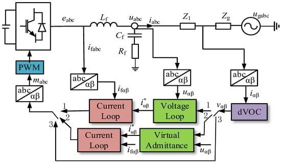
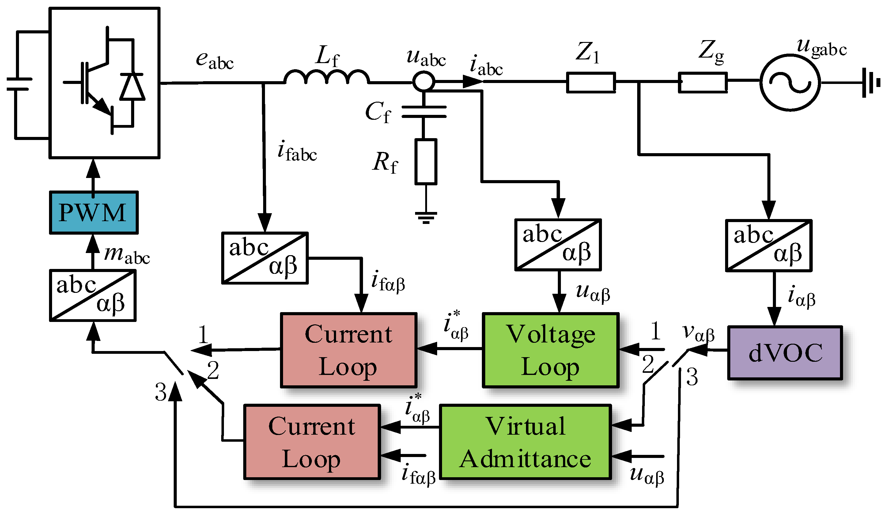
Figure 1 illustrates the main circuit topology and control architecture of a grid-connected inverter employing dVOC, where the proposed structure incorporates three parallel control paths to enable a unified analysis framework for various grid-forming implementations. It should be emphasized that these configurations are entirely independent; in practice, a single configuration is selected and fixed prior to operation, and no dynamic mode-switching is involved. Specifically, when Control Path I is selected, the grid current is processed by the dVOC outer loop to generate a voltage reference vector, which is subsequently tracked by a dual-loop voltage–current controller (DLC) to produce the final modulation signal, a configuration hereafter referred to as the dVOC–DLC structure. Similarly, in the case where Control Path II is selected, the voltage reference generated by the dVOC outer loop is fed into a virtual admittance control (VAC) module to generate the modulation signal, referred to as the dVOC–VAC structure. Lastly, if Control Path III is selected, the voltage reference produced by the dVOC outer loop is directly applied to the modulation stage without any inner-loop regulation, which is denoted as the open-loop dVOC structure.

Figure 1. The main circuit topology and control architecture.

In Figure 1, V_dc represents the DC-side voltage source, e_abc denotes the bridge-leg output voltage in the abc frame, u_abc and u_αβ are the inverter output voltages expressed in the abc and αβ reference frames, respectively. The filter inductor currents are denoted by i_fabc and i_fαβ, while i_abc and i_αβ represent the inverter output currents. The grid voltage is denoted by u_gabc. The parameters L_f, C_f, and R_c correspond to the filter inductance, filter capacitance, and damping resistor, respectively. The transmission line and grid impedances are modeled as Z₁ = R₁ + jω_nL₁ and Z_g = R_g + jω_nL_g, respectively, where R₁, R_g and L₁, L_g denote their corresponding resistances and inductances.

The outer-loop voltage reference generated by dVOC is denoted as v_αβ, while the current reference generated by either the voltage loop or the virtual admittance loop is denoted as $i_{\alpha \beta }^{\ast }$. The modulation voltage in the abc frame is denoted by m_abc, and the PWM block represents the pulse-width modulation module.

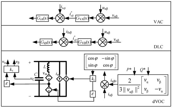
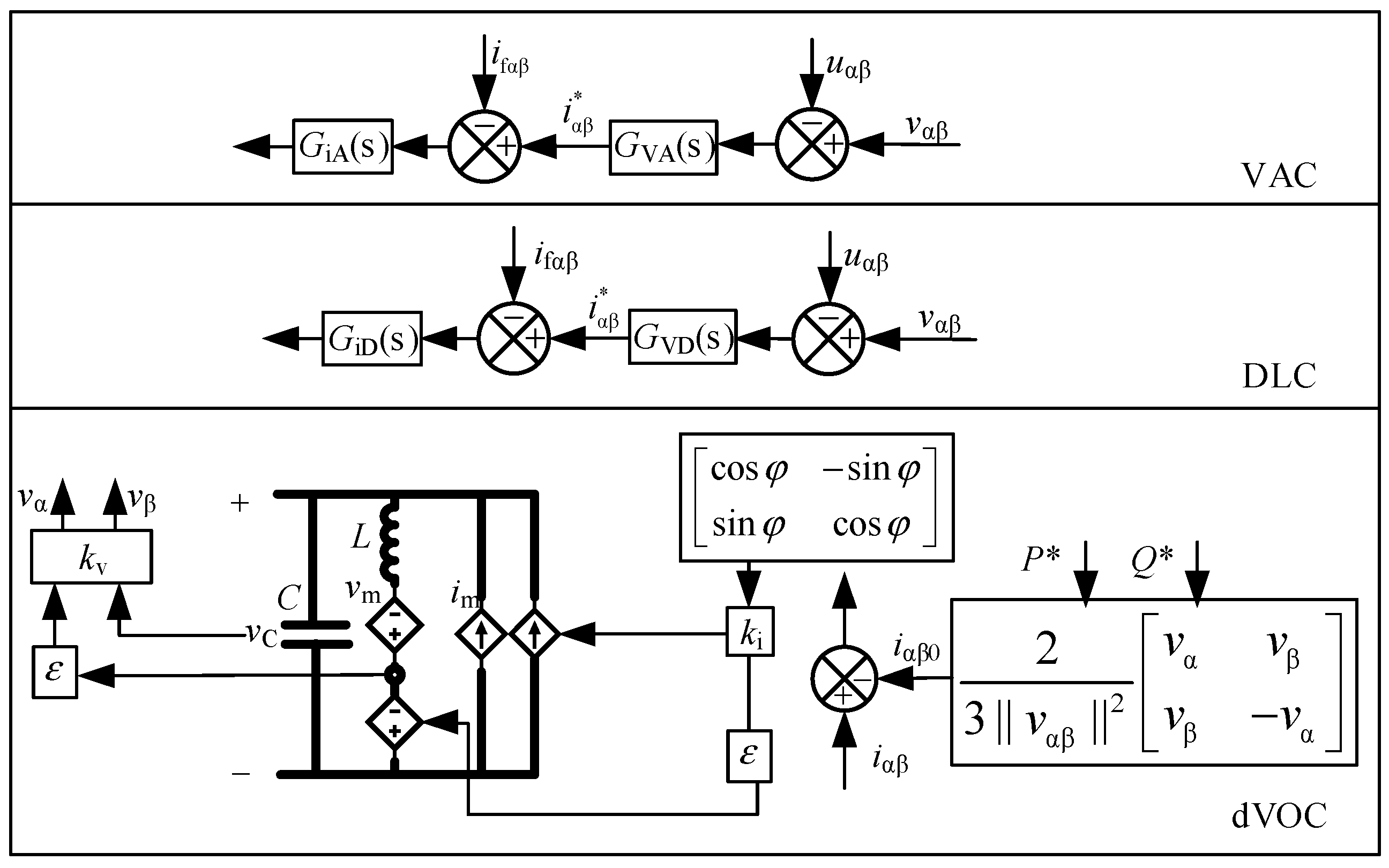
Figure 2 presents the control block diagram of dVOC and its associated inner-loop control structures. In the dVOC framework, L and C represent the virtual inductance and virtual capacitance, respectively, while P^∗ and Q^∗ denote the active and reactive power references.

Figure 2. The dVOC and inner-loop control structure.

The variable i_αβ0 represents the current reference in the αβ frame. The parameter $\epsilon =\sqrt{L/C}$ defines the characteristic impedance of the virtual oscillator. The transformation matrix R(φ) = $\left[\begin{array}{cc}cos\phi & -sin\phi \\ sin\phi & cos\phi \end{array}\right]$ and the rotation angle φ are defined accordingly, with φ = π/2 adopted in this study. The coefficients kv and ki represent the voltage and current scaling factors of the oscillator, while i_m and v_m denote the nonlinear current and voltage sources, respectively. The voltage across the virtual capacitor is denoted as v_C.

The open-loop transfer functions of the voltage and current controllers are defined to characterize the inner-loop dynamics. For the DLC structure, G_VD(s) and G_iD(s) represent the voltage and current regulators, respectively. Similarly, the inner-loop current controller for the VAC structure is denoted by G_iA(s). Distinctively, in the VAC architecture, the voltage-loop regulator G_VA(s) functions as a virtual admittance. To achieve flexible reshaping of the inverter’s output impedance, G_VD(s) is implemented using a Complex Proportional (CP) controller. By introducing a complex gain, this controller effectively regulates the damping characteristics of the terminal impedance within the target frequency band. These controller transfer functions are given by:

$$\left\{\begin{array}{l}{G}_{\mathrm{VD}}\left(s\right)=k_{\mathrm{pv}}+{\displaystyle \frac{2k_{\mathrm{rv}}{\omega }_{\mathrm{r}}s}{s^2+2{\omega }_{\mathrm{r}}s+{\omega }_0^2}}\\ G_{\mathrm{iD}}\left(s\right)=k_{\mathrm{pii}}\\ G_{\mathrm{VA}}\left(s\right)={\displaystyle \frac{1}{R_{\mathrm{v}}+\mathrm{j}{\omega }_0{L}_{\mathrm{v}}}}\\ G_{\mathrm{iA}}\left(s\right)=k_{\mathrm{pi}}+{\displaystyle \frac{2k_{\mathrm{ri}}{\omega }_{\mathrm{r}}s}{s^2+2{\omega }_{\mathrm{r}}s+{\omega }_0^2}}\end{array}\right.$$

(1)

where k_pv and k_rv are the proportional and resonant gains of the DLC voltage loop, k_pii is the proportional gain of the DLC current loop, Rv and L_v denote the virtual resistance and inductance in the virtual admittance loop, k_pi and k_ri are the proportional and resonant gains of the VAC current loop, ω_r is the resonant bandwidth angular frequency, and ω₀ is the resonant center angular frequency. The dVOC dynamics in the αβ frame are described as

$$\left[\begin{array}{c}{\dot{v}}_{\mathrm{\alpha }}\\ {\dot{v}}_{\mathrm{\beta }}\end{array}\right]=\left[\begin{array}{cc}(\xi /k_{\mathrm{v}}^2)\left(2V_{\mathrm{n}}^2-{‖v_{\mathrm{\alpha }\mathrm{\beta }}‖}^2\right)& -{\omega }_0\\ {\omega }_0& (\xi /k_{\mathrm{v}}^2)\left(2V_{\mathrm{n}}^2-{‖v_{\mathrm{\alpha }\mathrm{\beta }}‖}^2\right)\end{array}\right]\left[\begin{array}{c}{v}_{\mathrm{\alpha }}\\ v_{\mathrm{\beta }}\end{array}\right]-{\displaystyle \frac{k_{\mathrm{v}}{k}_{\mathrm{i}}}{C}}R\left(\phi \right)\left[\begin{array}{c}{i}_{\mathrm{\alpha }}-i_{\mathrm{\alpha }0}\\ i_{\mathrm{\beta }}-i_{\mathrm{\beta }0}\end{array}\right]$$

(2)

where V_n denotes the nominal RMS voltage magnitude of the inverter, v_αβ is the actual PCC voltage magnitude, and ξ is the convergence rate coefficient. The current reference is obtained as

$$\left[\begin{array}{c}{i}_{\mathrm{\alpha }0}\\ i_{\mathrm{\beta }0}\end{array}\right]={\displaystyle \frac{2}{3{‖v_{\mathrm{\alpha }\mathrm{\beta }}‖}^2}}\left[\begin{array}{cc}{v}_{\mathrm{\alpha }}& v_{\mathrm{\beta }}\\ v_{\mathrm{\beta }}& v_{\mathrm{\alpha }}\end{array}\right]\left[\begin{array}{c}{P}^{*}\\ Q^{*}\end{array}\right]$$

(3)

The voltage magnitude V and phase angle θ of v_αβ are given by β

$$\left\{\begin{array}{c}V={\displaystyle \frac{1}{\sqrt{2}}}{\left(v_{\mathrm{\alpha }}^2+v_{\mathrm{\beta }}^2\right)}^{{\displaystyle \frac{1}{2}}}\\ \theta =\arctan \left({\displaystyle \frac{v_{\mathrm{\alpha }}}{v_{\mathrm{\beta }}}}\right)\end{array}\right.$$

(4)

Differentiating Equation (4) and substituting into Equation (2) yields the polar-coordinate representation of dVOC as

$$\left\{\begin{array}{l}\dot{V}={\displaystyle \frac{\xi }{k_{\mathrm{v}}^2}}V(2V_{\mathrm{n}}^2-2V^2)-{\displaystyle \frac{k_{\mathrm{v}}{k}_{\mathrm{i}}}{3CV}}(Q_{\mathrm{e}}-Q^{\ast })\\ \dot{\theta }={\omega }_0-{\displaystyle \frac{k_{\mathrm{v}}{k}_{\mathrm{i}}}{3C{V}^2}}(P_{\mathrm{e}}-P^{\ast })\end{array}\right.$$

(5)

where P_e and Q_e denote the actual active and reactive power.

Under open-loop dVOC control, the frequency-domain expression of the phase-a modulation signal is given by

$$M_{\mathrm{a}}\left(s\right)=V_{\mathrm{\alpha }}\left(s\right)=V\left(\mathrm{s}\right)\cos \theta \left(\mathrm{s}\right)$$

(6)

where $V_{\alpha }\left(s\right)$ denotes the frequency-domain representation of $v_{\alpha }$.

Under the dVOC–DLC structure, the phase-$a$ modulation signal is expressed as

$$M_{\mathrm{a}}\left(s\right)=\left[\left(V_{\mathrm{\alpha }}\left(s\right)-U_{\mathrm{\alpha }}\left(s\right)\right)G_{\mathrm{VD}}\left(s\right)-I_{\mathrm{\alpha }}\left(s\right)\right]G_{\mathrm{iD}}\left(s\right)$$

(7)

where $U_{\alpha }\left(s\right)$ and $I_{\alpha }\left(s\right)$ represent the frequency-domain expressions of $u_{\alpha }$ and $i_{\alpha }$, respectively.

Similarly, under the dVOC–VAC structure, the modulation signal is given by

$$M_{\mathrm{a}}\left(s\right)=\left[\left(V_{\mathrm{\alpha }}\left(s\right)-U_{\mathrm{\alpha }}\left(s\right)\right)G_{\mathrm{VA}}\left(s\right)-I_{\mathrm{\alpha }}\left(s\right)\right]G_{\mathrm{iA}}\left(s\right)$$

(8)

2.2. Sequence Impedance Modeling

To facilitate stability assessment and avoid redundancy, this paper focuses on the positive-sequence impedance, since the negative-sequence impedance has been shown to always satisfy the Nyquist criterion under balanced operating conditions. Based on the inverter main circuit shown in Figure 1, the frequency-domain expression of the phase-a main circuit is derived as

$$E_{\mathrm{a}}\left(s\right)=U_{\mathrm{a}}\left(s\right)+s{L}_{\mathrm{f}}{I}_{\mathrm{a}}\left(s\right)$$

(9)

where E_a(s) = K_PWMG_d(s) M_a(s), U_a(s), E_a(s) and I_a(s) denote the frequency-domain expressions of the corresponding variables, and K_PWM is the modulation gain.

2.2.1. Sequence Impedance Modeling of GFM Control

Under the condition of a balanced three-phase system, the positive-sequence component at a given frequency can be equivalently represented by the negative-sequence component at the corresponding negative frequency, and the positive- and negative-sequence impedances exhibit complex conjugate symmetry. Specifically, the positive-sequence impedance Z_p(s) and negative-sequence impedance Z_n(s)satisfy Z_p(s) = Z_n(s). According to impedance-based stability theory, both the positive-sequence impedance ratio Z_p(s)/Z_g(s) and the negative-sequence impedance ratio Z_n(s)/Z_g(s) should theoretically satisfy the Nyquist stability criterion. However, it has been demonstrated in [26] that the negative-sequence subsystem typically exhibits a high stability margin and consistently satisfies the Nyquist criterion under balanced steady-state operation. Thus, the system’s stability boundary and oscillation damping are predominantly determined by the positive-sequence impedance ratio.

Accordingly, this paper focuses on the derivation and analysis of the positive-sequence impedance model of GFM inverters.

Before detailing the mathematical derivations, it is necessary to explicitly state the underlying assumptions of the proposed sequence impedance models. First, the modeling process is based on harmonic linearization around a stable steady-state operating point, where second-order and higher-order small perturbations (e.g., in the power calculation loops) are generally neglected. Second, actuator nonlinearities, such as PWM saturation, are not considered, as the converter is assumed to operate within its linear modulation range under small-signal conditions. Lastly, it should be noted that digital control and sampling delays are explicitly incorporated into the model, rather than being omitted. This is because these delays can significantly influence the mid-to-high frequency impedance phase characteristics, which are crucial for the stability assessment in this study.

By injecting a positive-sequence voltage perturbation at frequency f_p at the point of common coupling (PCC), the phase-$a$ voltage and current can be expressed as

$$\left\{\begin{array}{l}{v}_{\mathrm{a}}(t)=V_1\cos \left(2\mathrm{\pi }{f}_{1}t\right)+V_{\mathrm{p}}\cos \left(2\mathrm{\pi }{f}_{1}t+{\mathrm{\phi }}_{\mathrm{vp}}\right)\\ i_{\mathrm{a}}(t)=I_1\cos \left(2\mathrm{\pi }{f}_{1}t+{\mathrm{\phi }}_{\mathrm{i}1}\right)+I_{\mathrm{p}}\cos \left(2\mathrm{\pi }{f}_{1}t+{\mathrm{\phi }}_{\mathrm{ip}}\right)\end{array}\right.$$

(10)

where $V_1$ and $V_p$ denote the peak values of the fundamental component and the positive-sequence perturbation voltage, respectively, and $I_1$ and $I_p$ denote the corresponding current components. The variables $f_1$ and $f_p$ represent the fundamental frequency and perturbation frequency, respectively, while ${\phi }_{vp}$, ${\phi }_{i1}$, and ${\phi }_{ip}$ denote the initial phase angles of the voltage and current components.

Applying the Clarke transformation to Equation (10), the voltage and current in the $\alpha \beta$ frame is obtained as

$$\left\{\begin{array}{l}{V}_{\mathsf{\alpha }}[f]=\left\{\begin{array}{l}{\mathit{V}}_1,f=f_1\\ {\mathit{V}}_{\mathrm{p}},f=f_{\mathrm{p}}\end{array}\right.\\ V_{\mathrm{\beta }}[f]=\left\{\begin{array}{l}-\mathrm{j}{\mathit{V}}_1,f=f_1\\ -\mathrm{j}{\mathit{V}}_{\mathrm{p}},f=f_{\mathrm{p}}\end{array}\right.\end{array}\right.$$

(11)

$$\left\{\begin{array}{l}{I}_{\mathrm{\alpha }}[f]=\left\{\begin{array}{l}{\mathit{I}}_1, f=f_1\\ {\mathit{I}}_{\mathrm{p}}, f=f_{\mathrm{p}}\end{array}\right.\\ I_{\mathrm{\beta }}[f]=\left\{\begin{array}{l}-\mathrm{j}{\mathit{I}}_1, f=f_1\\ -\mathrm{j}{\mathit{I}}_p, f=f_{\mathrm{p}}\end{array}\right.\end{array}\right.$$

(12)

where $V_1=V_1/2$, $V_{\mathrm{p}}=\left(V_{\mathrm{p}}/2\right){\mathrm{e}}^{{\mathrm{j}\mathrm{\phi }}_{\mathrm{vp}}}$, ${\mathrm{I}}_1=\left(I_1/2\right){\mathrm{e}}^{{\mathrm{j}\mathrm{\phi }}_{\mathrm{i}1}}$, ${\mathrm{I}}_{\mathrm{p}}=\left(I_{\mathrm{p}}/2\right){\mathrm{e}}^{{\mathrm{j}\mathrm{\phi }}_{\mathrm{ip}}}$ are defined accordingly.

Based on instantaneous power theory, the instantaneous power of a three-phase system is expressed as

$$\left\{\begin{array}{l}P={\displaystyle \frac{3}{2}}\left(v_{\mathrm{\alpha }}{i}_{\mathrm{\alpha }}+v_{\mathrm{\beta }}{i}_{\mathrm{\beta }}\right)\\ Q={\displaystyle \frac{3}{2}}\left(v_{\mathrm{\beta }}{i}_{\mathrm{\alpha }}-v_{\mathrm{\alpha }}{i}_{\mathrm{\beta }}\right)\end{array}\right.$$

(13)

Substituting (11) and (12) into (13) and neglecting higher-order perturbation terms, the frequency-domain expressions for active and reactive power are derived based on the convolution theorem as follows:

$$P_{\mathrm{e}}(s)=\left\{\begin{array}{ll}3{\mathit{V}}_1{I}_1{\cos \mathrm{\phi }}_{\mathrm{i}1},\mathrm{dc}\hfill & \\ 3({\mathit{V}}_1{\mathit{I}}_{\mathrm{p}}+{\mathit{I}}_1^{*}{\mathit{V}}_{\mathrm{p}}),\hfill & f=f_{\mathrm{p}}-f_1\hfill \end{array}\right.$$

(14)

$$Q_{\mathrm{e}}(s)=\left\{\begin{array}{ll}-3{\mathit{V}}_1{I}_1{\sin \mathrm{\phi }}_{\mathrm{i}1},\mathrm{dc}\hfill & \\ 3\mathrm{j}({\mathit{V}}_1{\mathit{I}}_{\mathrm{p}}-{\mathit{I}}_1^{*}{\mathit{V}}_{\mathrm{p}}),\hfill & f=f_{\mathrm{p}}-f_1\hfill \end{array}\right.$$

(15)

Substituting (14) and (15) into (5) yields the frequency-domain expressions for the small-signal perturbations of phase angle and voltage magnitude, as shown in (16):

$$\left\{\begin{array}{l}\Delta \theta \left(\mathrm{s}\right)=-3D\left(s\right){\mathit{V}}_1{\mathit{I}}_{\mathrm{p}}-3\mathrm{D}\left(s\right){\mathit{I}}_1^{*}{\mathit{V}}_{\mathrm{p}},f=f_{\mathrm{p}}\\ \Delta V\left(\mathrm{s}\right)=-3\mathrm{j}N\left(s\right){\mathit{V}}_1{\mathit{I}}_{\mathrm{p}}+3\mathrm{j}N\left(s\right){\mathit{I}}_1^{*}{\mathit{V}}_{\mathrm{p}},f=f_{\mathrm{p}}\end{array}\right.$$

(16)

where $D(s)={\displaystyle \frac{2k_{\mathrm{v}}{k}_{\mathrm{i}}}{3C{V}^{2}s}}$, $N(s)={\displaystyle \frac{2k_{\mathrm{v}}^3{k}_{\mathrm{i}}}{3CV(k_{\mathrm{v}}^{2}s+\epsilon V_1^2)}}$ are defined accordingly.

The small-signal expression of the modulation signal is given by

$$\Delta M_{\mathrm{a}}(s)=\Delta V(s)\cos {\theta }_0-\Delta \theta (s)\sin {\theta }_0{V}_0$$

(17)

where $V_0$ denotes the fundamental component of the modulation voltage, θ₀ is 2πf₁,

Equation (17) can be rewritten as:

$$\Delta M_{\mathrm{a}}(s)={\displaystyle \frac{1}{2}}\Delta V(s-\mathrm{j}{\omega }_0)+{\displaystyle \frac{\mathrm{j}}{2}}{V}_0\Delta \theta (s-\mathrm{j}{\omega }_0)$$

(18)

By substituting (16) into (18), the modulation signal of the open-loop dVOC structure is obtained:

$$\begin{array}{l}\Delta M_{\mathrm{a}}(s)=-A(s-\mathrm{j}{\omega }_0){\mathit{V}}_p-B(s-\mathrm{j}{\omega }_0){\mathit{I}}_p\\ \end{array}$$

(19)

where

$$A(s-\mathrm{j}{\omega }_0)={\displaystyle \frac{3}{2}}\mathrm{j}[N(s-\mathrm{j}{\omega }_0)-V_{1}D(s-\mathrm{j}{\omega }_0\left)\right], B(s-\mathrm{j}{\omega }_0)={\displaystyle \frac{3}{2}}\mathrm{j}[N(s-\mathrm{j}{\omega }_0)+V_{1}D(s-\mathrm{j}{\omega }_0)]$$

Substituting (19) into (9) yields the small-signal voltage equation of the main circuit as:

$$K_{\mathrm{PWM}}{G}_d\left(s\right)\Delta M_{\mathrm{a}}(s)={\mathrm{V}}_{\mathrm{p}}+s{L}_{\mathrm{f}}{\mathit{I}}_{\mathrm{p}}$$

(20)

Rearranging (20) and incorporating the filter capacitor branch yields the sequence impedance model of the open-loop dVOC structure as (21), where the filter capacitor branch is expressed as: $Z_{\mathrm{cf}}=R_{\mathrm{c}}+1/\mathrm{s}{C}_{\mathrm{f}}$.

$$Z_{\mathrm{Pd}}=-{\displaystyle \frac{V_{\mathrm{p}}}{I_{\mathrm{p}}}}={\displaystyle \frac{s{L}_{\mathrm{f}}+\mathrm{j}1.5K_{\mathrm{PWM}}\left[V_{1}D\left(s-\mathrm{j}{\omega }_0\right)+N\left(s-\mathrm{j}{\omega }_0\right)\right]V_1}{\mathrm{j}1.5K_{\mathrm{PWM}}\left[V_{1}D\left(s-\mathrm{j}{\omega }_0\right)-N\left(s-\mathrm{j}{\omega }_0\right)\right]I_1^{\ast }+1}}//Z_{\mathrm{cf}}$$

(21)

where // denotes parallel connection.

When inner loops are incorporated into the converter control scheme, substituting the outer-loop modulation signal into (8) and (9) yields the modulation signal expressions for the DLC and VAC structures as (22) and (23), respectively:

$$\Delta M_{\mathrm{a}-\mathrm{DLC}}(s)=G_{\mathrm{iD}}\left(s\right)G_{\mathrm{VD}}\left(s\right)\left[A\left(s-\mathrm{j}{\omega }_0\right)I_1^{\ast }+1\right]{\mathit{V}}_{\mathrm{p}}-G_{\mathrm{iD}}\left(s\right)\left[B\left(s-\mathrm{j}{\omega }_0\right)V_1{G}_{\mathrm{VD}}\left(s\right)-1\right]{\mathit{I}}_{\mathrm{p}}$$

(22)

$$\Delta M_{\mathrm{a}-\mathrm{VAC}}(s)=G_{\mathrm{iA}}\left(s\right)G_{\mathrm{VA}}\left(s\right)\left[A\left(s-\mathrm{j}{\omega }_0\right)I_1^{\ast }+1\right]{\mathit{V}}_{\mathrm{p}}-G_{\mathrm{iA}}\left(s\right)\left[B\left(s-\mathrm{j}{\omega }_0\right)V_1{G}_{\mathrm{VA}}\left(s\right)-1\right]{\mathit{I}}_{\mathrm{p}}$$

(23)

Substituting (22) and (23) into (20) and incorporating the filter capacitor branch yields the impedance models for the DLC and VAC structures as (24) and (25), respectively:

$$Z_{\mathrm{PD}}={\displaystyle \frac{s{L}_{\mathrm{f}}-K_{\mathrm{PWM}}{G}_{\mathrm{iD}}\left(s\right)\left[B\left(s-\mathrm{j}{\omega }_0\right)V_1{G}_{\mathrm{VD}}\left(s\right)-1\right]}{1+K_{\mathrm{PWM}}{G}_{\mathrm{iD}}\left(s\right)G_{\mathrm{VD}}\left(s\right)\left[A\left(s-\mathrm{j}{\omega }_0\right)I_1^{\ast }+1\right]}}//Z_{\mathrm{cf}}$$

(24)

$$Z_{\mathrm{PA}}={\displaystyle \frac{s{L}_{\mathrm{f}}-K_{\mathrm{PWM}}{G}_{\mathrm{iA}}\left(s\right)\left[B\left(s-\mathrm{j}{\omega }_0\right)V_1{G}_{\mathrm{VA}}\left(s\right)-1\right]}{1+K_{\mathrm{PWM}}{G}_{\mathrm{iA}}\left(s\right)G_{\mathrm{VA}}\left(s\right)\left[A\left(s-\mathrm{j}{\omega }_0\right)I_1^{\ast }+1\right]}}//Z_{\mathrm{cf}}$$

(25)

2.2.2. Frequency-Sweep Validation

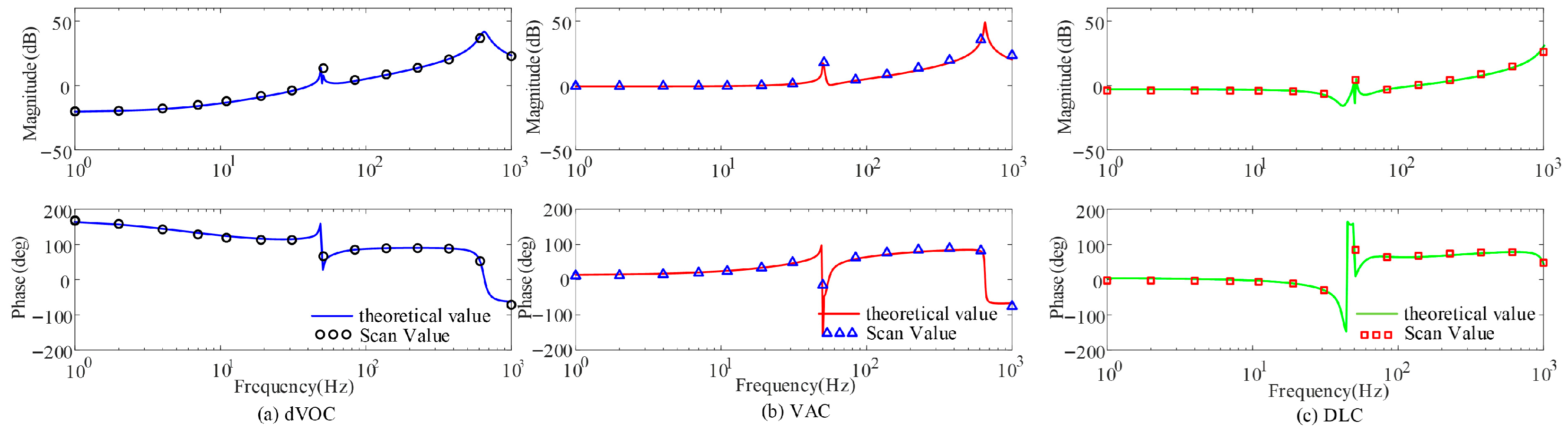
To validate the accuracy of the derived impedance models, frequency-sweep tests are conducted on the MATLAB R2022b/Simulink platform using the system parameters listed in Table 1. The comparison between the theoretical impedance curves and the simulation-based sweep results is shown in Figure 3. The close agreement confirms the validity of the proposed sequence impedance models.

Table 1. Key system parameters.

Parameters	Symbols	Value
DC Voltage	Vdc	700 V
Grid Voltage	Ug	311 V
Rated Capacity	Sn	10 kVA
Filter Inductance	Lf	3 mH
Filter Capacitor	Cf	20 uF
Damping Resistor	Rc	1.5 Ω
Switching Frequency	fs	10 kHz
Virtual Capacitance	C	0.4
Current Compression Factor	kv	220
Current Scaling Factor	ki	0.044
Virtual Resistance	Rv	1.4 Ω
Virtual Inductance	Lv	13.6 mH
DLC Voltage Loop Proportionality Factor	kpv	1
DLC Voltage Loop Resonance Factor	kiv	50
DLC Current Loop Proportionality Factor	kpii	4
Resonance Center Angular Frequency	ωr	π/2
VAC Current Loop Proportionality Factor	kpi	1
VAC Current Loop Resonance Factor	kri	30
Proportional Coefficient of PLL	kppll	0.2659
Integral Coefficient of PLL	kipll	10.998
GFL Current Loop Proportionality Factor	kpc	0.0343
GFL Current Loop Integral Factor	kic	45.7143
Feedforward Factor	Kf	0.0029

Figure 3. Comparison of the theoretical positive-sequence impedance models and the simulation-based frequency sweep results for the three GFM control structures.

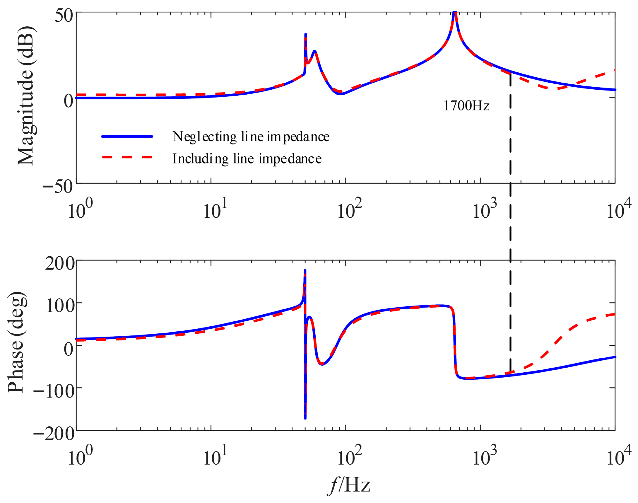
In addition to the inverter’s internal control dynamics, the physical characteristics of the connection to the main grid must also be considered in practical applications. Specifically, JKLYJ-120 aluminum-core cables with a uniform length of 200 m between low-voltage nodes are selected as the transmission lines in this study. While the inherent impedance of such lines implicitly forms an LCL filter structure with the inverter’s LC filter, frequency-domain analysis, as shown in Figure 4, indicates that the relatively small line inductance in these scenarios generally shifts the resulting resonance to the extremely high-frequency range. Consequently, this physical line effect falls well beyond the mid-to-high frequency band of interest. Therefore, the simplified LC model remains sufficiently accurate for characterizing the interactive stability, and the core comparative conclusions regarding the different inner-loop structures remain valid.

Figure 4. Impedance characteristics with and without considering the transmission line impedance.

2.2.3. Impedance Characteristics Under Different Control Structures

To investigate the dynamic interaction mechanisms in mixed inverter systems, the impedance characteristics of GFM inverters with different control structures are compared with those of a typical GFL inverter. The GFL impedance model is adopted from [27] and is given by

$$Z_{\mathrm{GFL}}(s)={\displaystyle \frac{s{L}_{\mathrm{f}}+\frac{V_{\mathrm{dc}}}{2}\left(H_{\mathrm{i}}\left(s-\mathrm{j}2\mathrm{\pi }{f}_1\right)-\mathrm{j}{K}_{\mathrm{d}}\right)}{1-\frac{V_{\mathrm{dc}}}{2}{K}_{\mathrm{f}}-\frac{V_{\mathrm{dc}}}{4}\frac{T_{\mathrm{PLL}}(s-\mathrm{j}2\mathrm{\pi }{f}_1)}{V_1}{G}_{\mathrm{d}}(s)H_{\mathrm{i}}\left(s-\mathrm{j}2\mathrm{\pi }{f}_1\right)(I_{\mathrm{d}}+\mathrm{j}{I}_{\mathrm{q}})}}$$

(26)

where the current controller is defined as $H_i\left(s\right)=k_{pc}+k_{ic}/s$, and the PLL transfer function is given by T_PLL(s) = H_PLL(s)/(1 + H_PLL(s)U₁), with H_PLL(s) = k_ppll + k_ipll/s. The parameters kpc, kic, kppll, and kipll denote the proportional and integral gains of the current controller and PLL, respectively. The variables K_d and K_f represent the decoupling and feedforward coefficients, while I_d and I_q denote the d and q-axis currents at the PCC.

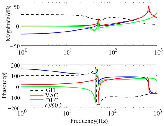
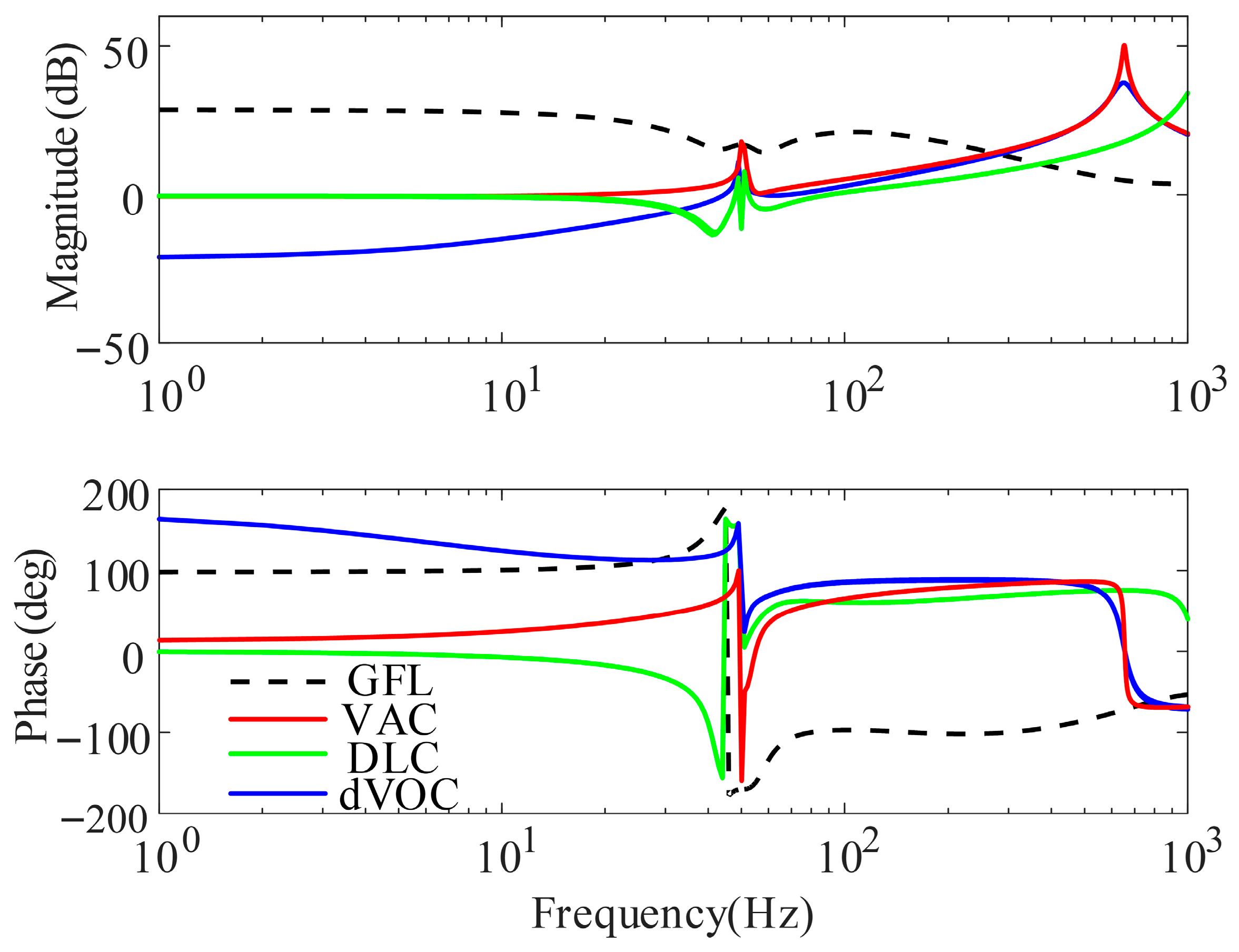
Figure 5 compares the impedance characteristics of GFM inverters with different inner-loop structures and the GFL inverter.

Figure 5. The impedance characteristics of GFM inverters with different inner-loop structures and the GFL inverter.

From the magnitude responses, it is observed that in the low- and medium-frequency range, the impedance magnitude of the GFL inverter is higher than that of the GFM inverters. As frequency increases, the impedance magnitude of the GFM inverter rises rapidly and eventually exceeds that of the GFL inverter. Among the GFM configurations, the structures equipped with inner-loop control (i.e., the DLC and VAC structures) exhibit relatively higher and more constant impedance magnitudes in the low-frequency range, whereas the open-loop structure exhibits a lower magnitude with more pronounced frequency dependence. In the medium- to high-frequency range, all GFM structures exhibit similar impedance trends, with minor differences primarily arising from the specific inner-loop implementation.

From the phase responses, the GFL inverter exhibits capacitive characteristics and a capacitive negative damping region (where the phase drops below −90°) in the medium- to high-frequency range. In contrast, the GFM inverters generally maintain inductive characteristics over a wide frequency range and do not exhibit this high-frequency capacitive negative damping. However, in the low-frequency range, although the GFL inverter does not exhibit negative damping, certain GFM structures (specifically, the DLC structure) may introduce negative damping due to specific inner-loop dynamics, potentially giving rise to new low-frequency oscillatory modes.

In mixed GFM–GFL systems, the inverters are connected in parallel, and the overall system impedance is dominated by the inverter with the lower impedance magnitude. When the GFM inverter exhibits a lower impedance magnitude than the GFL inverter and its phase does not contain capacitive negative damping regions, oscillations induced by the interaction between the GFL inverter and an inductive grid can be effectively suppressed. In practical systems, the capacity ratio between GFM and GFL inverters varies, which directly affects these equivalent impedance characteristics. The specific influence of this capacity ratio on system stability is further investigated quantitatively in Section 3.

3. Stability Analysis of Grid-Connected Systems

According to [27], the stability of a hybrid system composed of grid-following (GFL) and grid-forming (GFM) inverters relies on three necessary conditions: the GFL inverter must remain stable when connected to an ideal grid; the GFM inverter must be able to operate stably when connected to the grid independently; the impedance ratio between the inverter system and the grid must satisfy the Nyquist stability criterion.

Based on the preceding analysis, the stable operation of a standalone grid-connected GFM inverter constitutes a prerequisite for enhancing the stability of hybrid systems. Therefore, it is necessary to first investigate the stability characteristics of GFM inverters operating in single-inverter grid-connected scenarios.

3.1. Stability Analysis of Single GFM Grid-Connected Systems

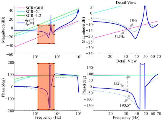
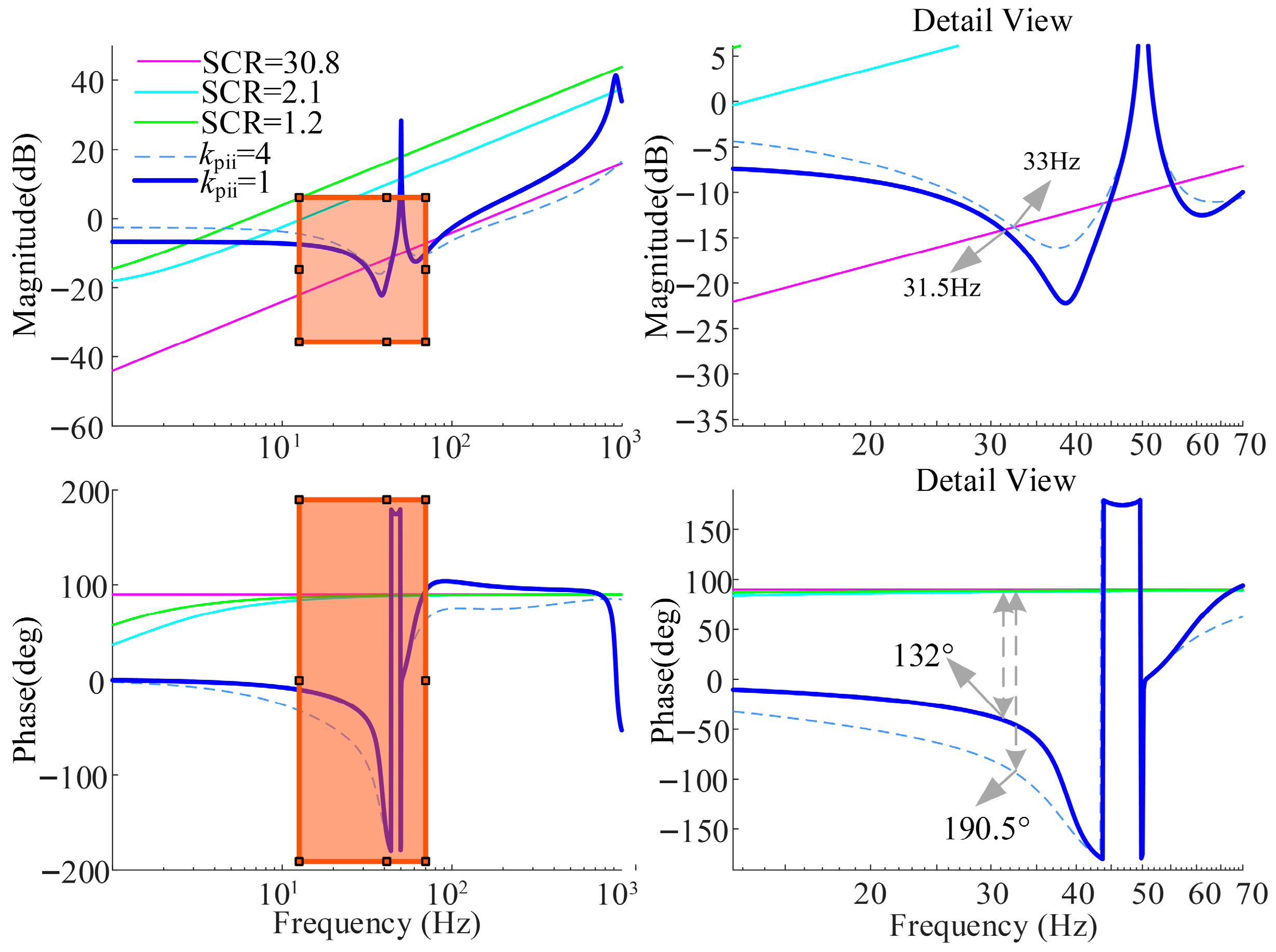
To evaluate the adaptability of different GFM control structures to grids with varying strengths, three representative grid conditions are considered by adjusting the short-circuit ratio (SCR): an extremely weak grid (SCR = 1.2), a weak grid (SCR = 2.1), and a strong grid (SCR = 30.8). The grid is modeled as an ideal voltage source in series with an equivalent impedance. Given the large number of parameters involved in the three GFM control structures investigated in this paper—namely, open-loop dVOC, dVOC with dual-loop control (DLC), and dVOC with virtual admittance control (VAC)—and considering that the primary objective is to establish sequence impedance models and reveal their stability implications in both standalone and hybrid systems, this subsection focuses on the proportional gain of the inner current loop in DLC and VAC as representative parameters.

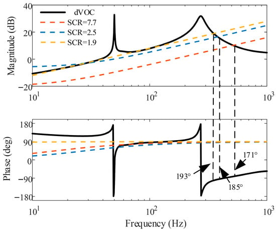
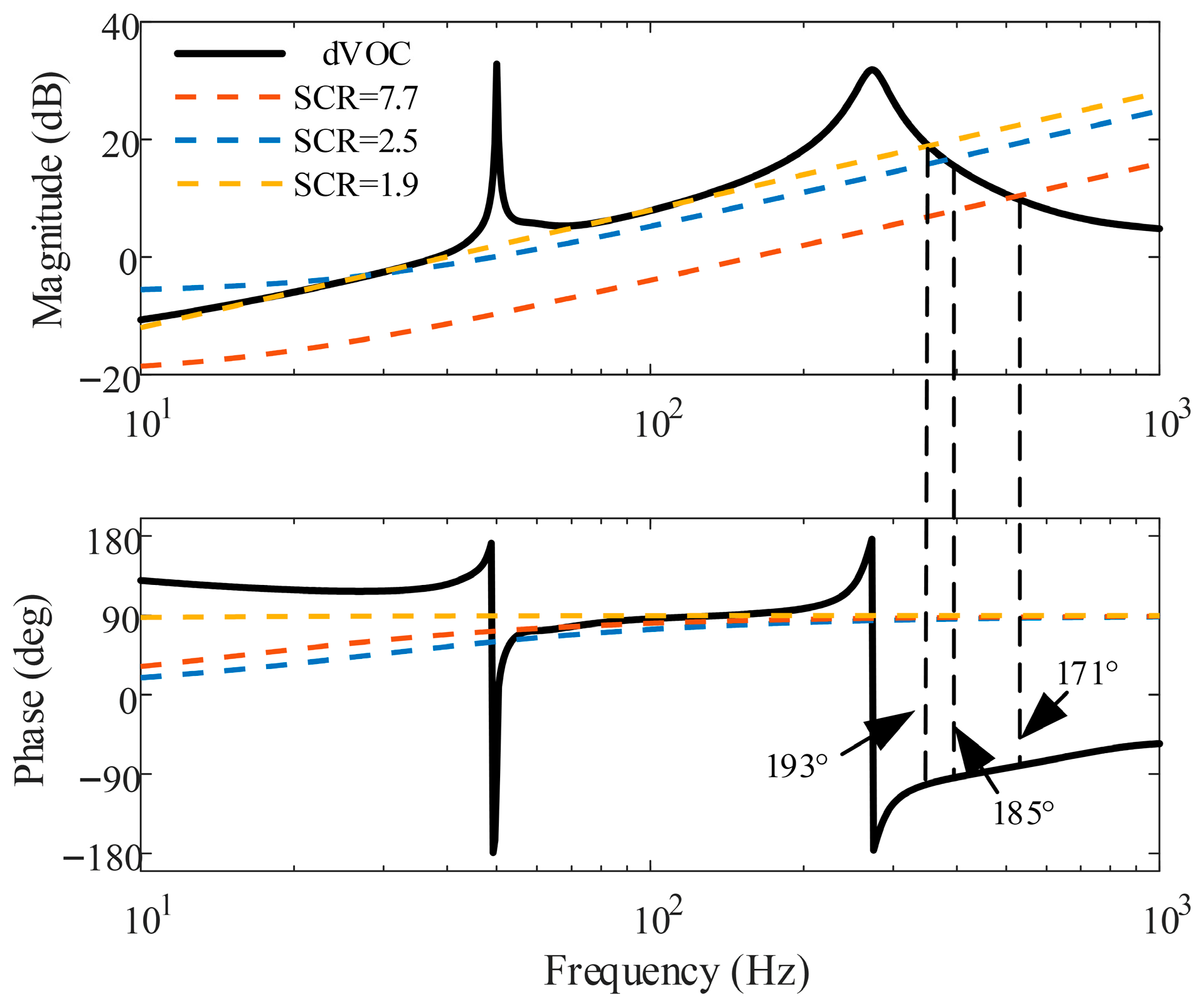
As shown in Figure 6, under weak (SCR = 2.1) and extremely weak grid conditions (SCR = 1.2), the magnitude intersection between the output impedance of the DLC-based GFM inverter and the grid impedance exhibits sufficient phase margin, satisfying the stability criterion. This indicates that DLC-controlled GFM inverters possess strong adaptability to weak grids.

Figure 6. DLC and grid impedance characteristics curve.

With increasing grid strength (e.g., SCR = 30.8), the intersection points between the grid impedance and the inverter output impedance gradually shift toward the fundamental frequency, as shown in Figure 7. When the current-loop proportional gain is set to k_pii = 4, the phase difference at the intersection exceeds 180°, violating the stability condition and leading to instability. By reducing k_pii to 1, the phase difference becomes smaller than 180°, and stable operation is restored. This demonstrates that reducing the current-loop proportional gain enhances the stability of DLC-based GFM inverters under strong grid conditions.

Figure 7. VAC and grid impedance characteristics curve.

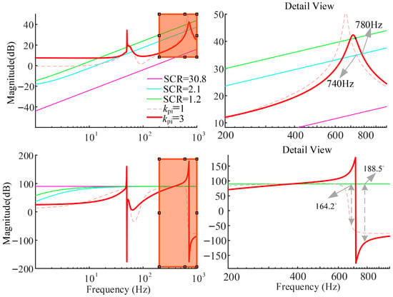
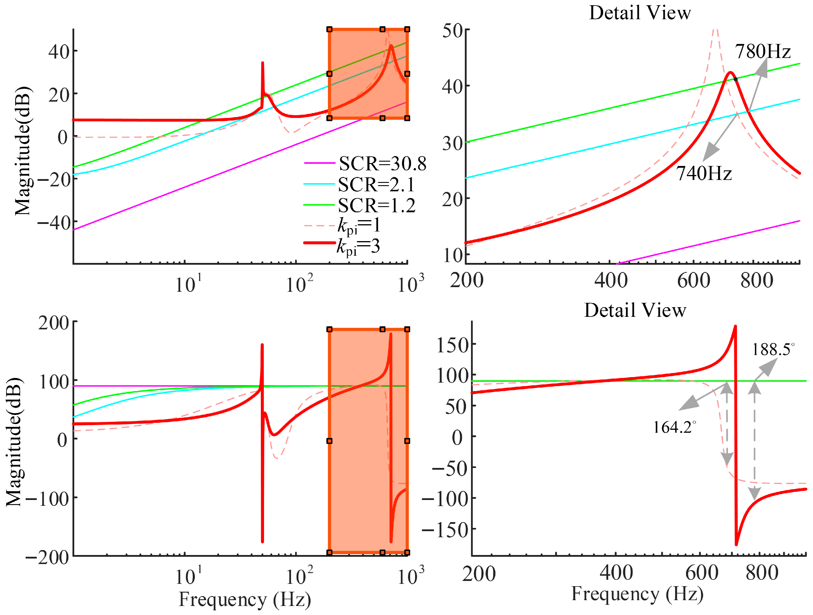
Figure 7 illustrates the impedance characteristics of VAC-controlled GFM inverters under different grid strengths and current-loop proportional gains. As the proportional gain kpi increases, a pronounced capacitive negative damping region emerges in the medium- and high-frequency ranges. Under strong grid conditions, the grid impedance is relatively small, and its intersection with the inverter impedance occurs at higher frequencies, far from the capacitive resonance peak. As a result, sufficient phase margin is maintained. However, under weak grid conditions, a large k_pi leads to insufficient phase margin and instability, whereas a smaller k_pi ensures stable operation.

These results indicate that reducing the current-loop proportional gain improves the stability of VAC-controlled GFM inverters in weak grid environments.

3.2. Stability Analysis of Hybrid GFM–GFL Systems

In weak grid conditions, GFL inverters inherently exhibit capacitive negative damping regions, which are detrimental to system stability. In hybrid GFM–GFL systems, however, GFM inverters can reshape the overall system impedance and enhance grid adaptability.

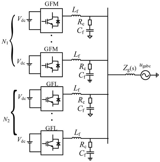
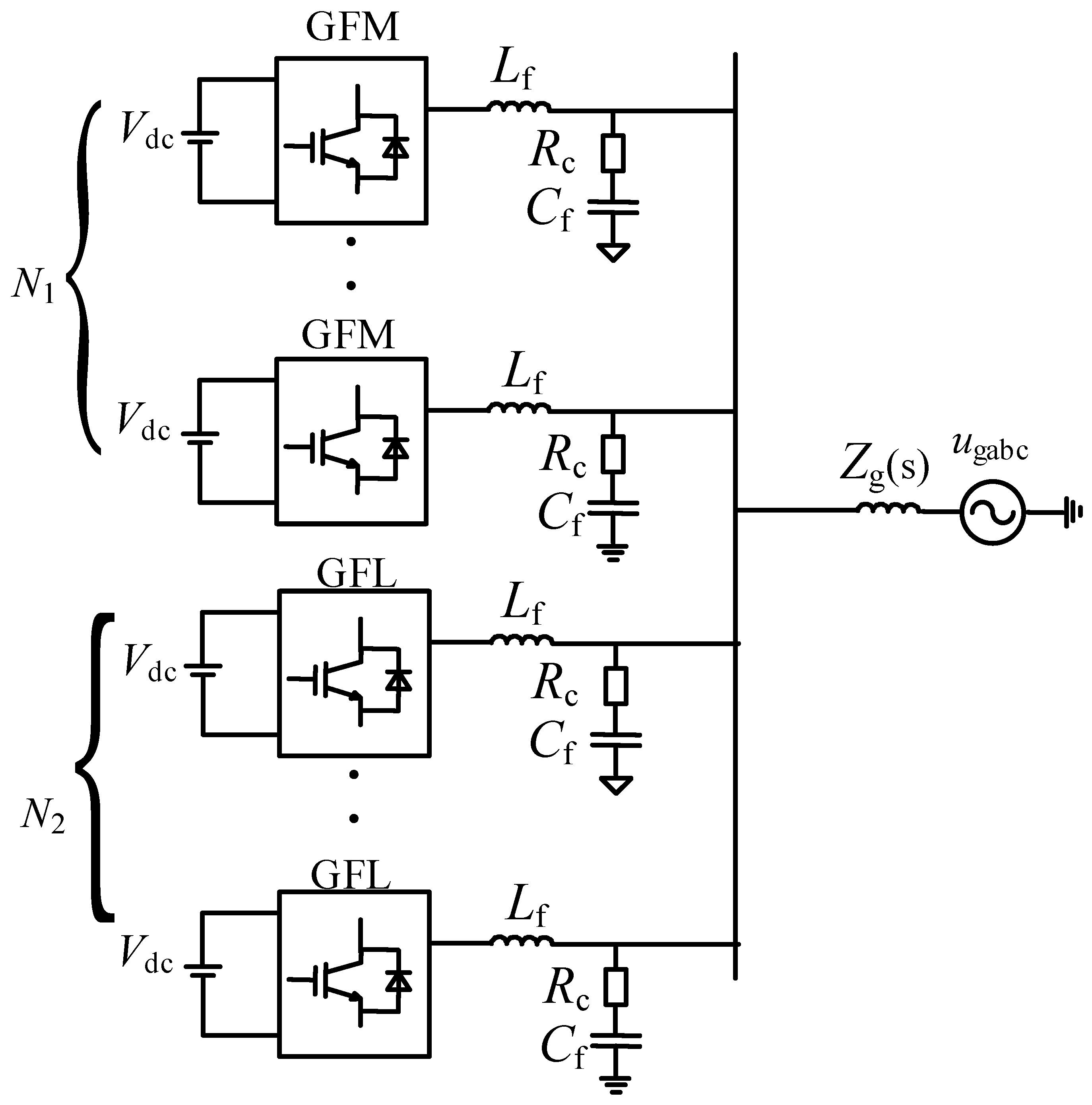
The topology of the hybrid system is shown in Figure 8. The equivalent output impedance of the hybrid system can be expressed as

$$Z_{\mathrm{H}}={\displaystyle \frac{Z_{\mathrm{GFL}}{Z}_{\mathrm{GFM}}}{N_1{Z}_{\mathrm{GFL}}+N_2{Z}_{\mathrm{GFM}}}}$$

(27)

where $N_1$ and $N_2$ denote the numbers of GFM and GFL inverters, respectively.

Figure 8. The topology of the hybrid system.

To focus on the stability interaction mechanisms, an aggregated modeling approach is adopted for the hybrid GFM-GFL system in Figure 7. It is assumed that the steady-state power sharing and circulation issues among parallel units are properly managed by higher-level control, allowing the analysis to prioritize the impedance-shaping effects of different inner loops on system damping.

$$\left\{\begin{array}{l}{T}_{\mathrm{M}1}=I_{\mathrm{c}}(s)+{\displaystyle \frac{V_{\mathrm{s}}(s)}{Z_{\mathrm{GFM}}(s)}}-{\displaystyle \frac{V_{\mathrm{g}}(s)}{Z_{\mathrm{H}}(s)}}\hfill \\ T_{\mathrm{M}2}={\displaystyle \frac{1}{1+Z_{\mathrm{g}}(s)/Z_{\mathrm{H}}(s)}}\hfill \end{array}\right.$$

(28)

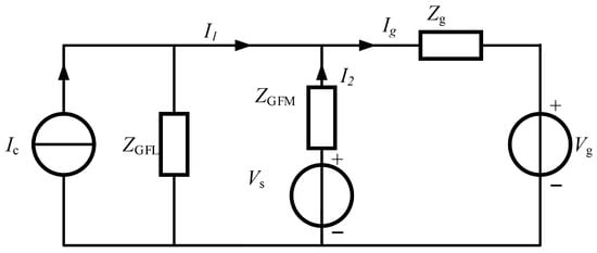
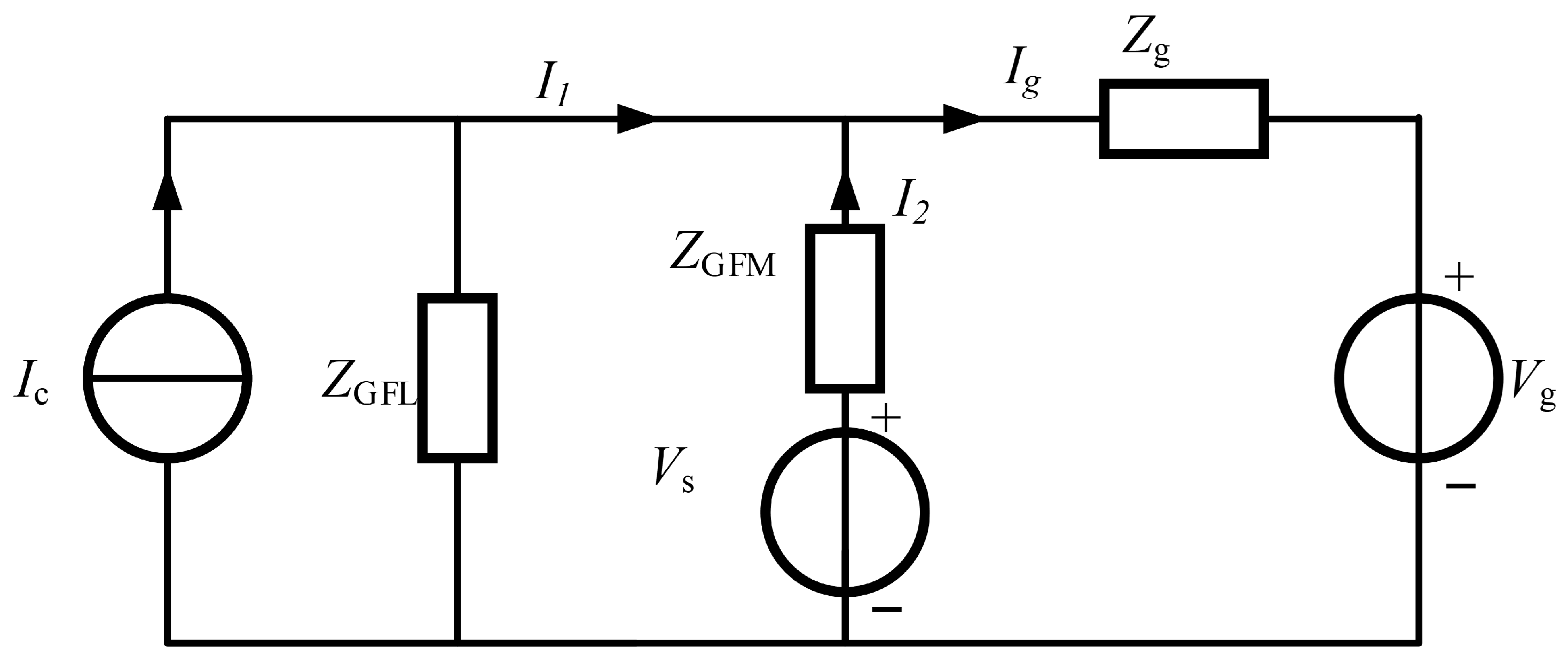
The stability of the AC transmission system for hybrid GFL- and GFM-based renewable energy plants is jointly determined by TF1 and TF2. Specifically, the system is small-signal stable if and only if all poles of both TF1 and TF2 are in the left-half plane (LHP). Regarding TF1, under the prerequisite that the GFL plant operates stably under an ideal grid (where all poles of Ic and 1/ZGFL reside in the LHP), its stability is primarily governed by Vs. Based on the equivalent analytical model shown in Figure 9. According to (28), Vs represents the open-circuit voltage at the GFL point of interconnection (POl), which is equivalent to the terminal voltage when the GFM station is connected to the grid independently. Provided that the GFM station maintains stability in standalone grid-connected mode, all poles of TF1 are guaranteed to lie in the LHP. For TF2, all its poles are in the LHP if and only if the open-loop transfer function Zg/ZH satisfies the Nyquist stability criterion [28].

Figure 9. Equivalent impedance model of hybrid system.

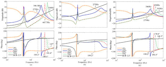
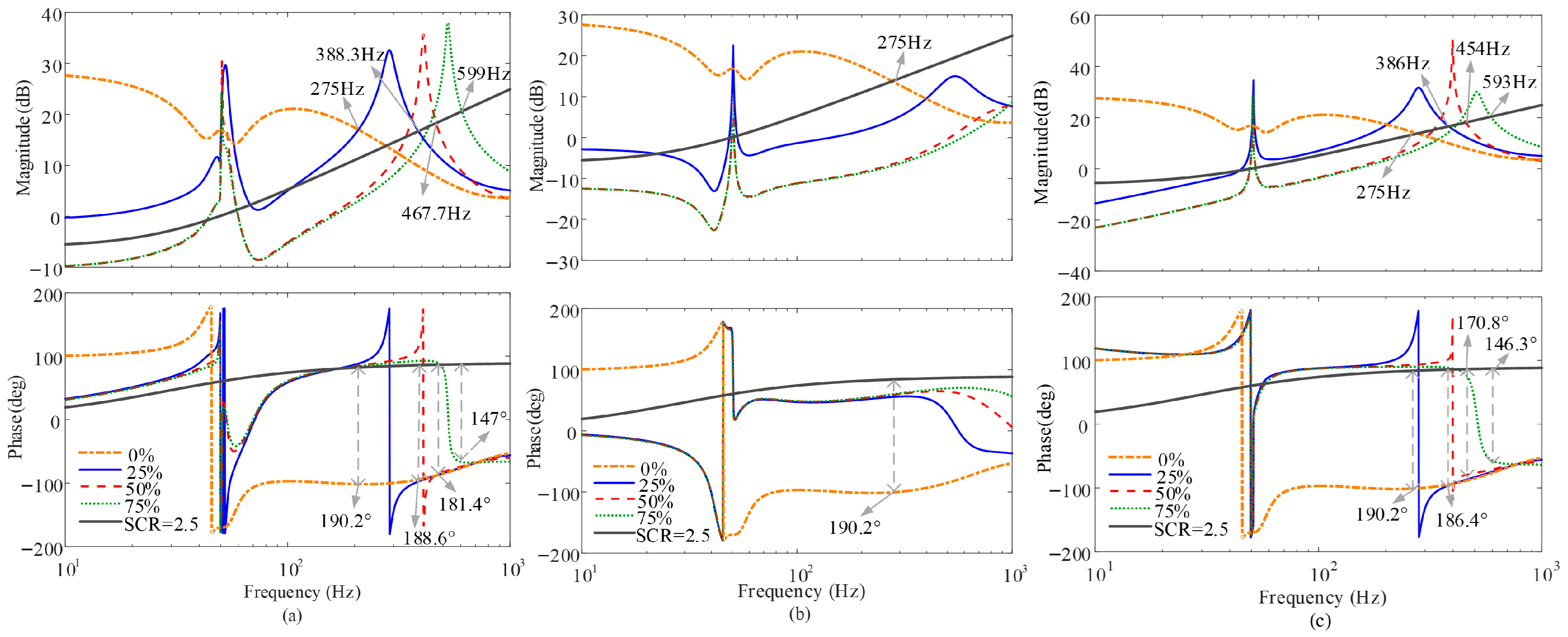
Figure 10 compares the impedance characteristics of hybrid systems under different GFM capacity ratios for the VAC, DLC, and open-loop structures, given a total number of inverters N = 4 and an SCR of 2.5. When the GFM capacity ratio is 0% (i.e., a pure GFL system), the hybrid system exhibits capacitive negative damping over a wide frequency range, rendering it highly susceptible to medium-frequency oscillations. As the GFM capacity ratio increases from 25% to 75%, the resonance peaks gradually shift toward higher frequencies, and the phase margin at the impedance intersection points is progressively improved.

Figure 10. Comparison of impedance curves for mixed-connection systems under different controls. (a): VAC; (b): DLC; (c): dVOC.

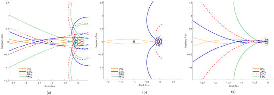
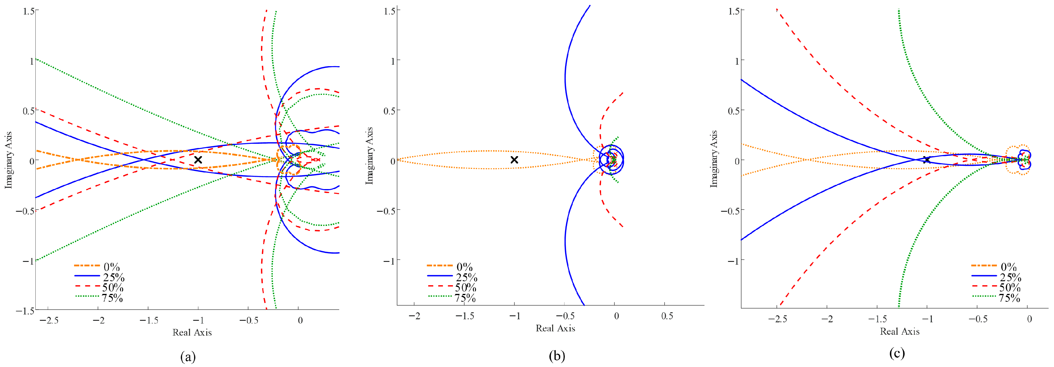
Specifically, in the VAC–GFL hybrid system, stability under SCR = 2.5 is achieved only when the GFM capacity ratio reaches 75%. At this specific ratio, the phase difference at the magnitude intersection is reduced to less than 180° (Figure 10a), and the corresponding Nyquist contour formally ceases to encircle the (−1, j0) point (Figure 11a). In striking contrast, the DLC–GFL hybrid system realizes stable operation with only a 25% GFM capacity ratio. As shown in Figure 10b, no magnitude intersection occurs within the unstable phase region, a stability condition rigorously confirmed by the Nyquist plot (Figure 11b), which indicates zero encirclements of the (−1, j0) point.

Figure 11. Comparison of Nyquist curves for mixed-connection systems under different controls. (a): VAC; (b): DLC; (c): dVOC.

For the open-loop GFM–GFL hybrid system, a minimum GFM capacity ratio of 50% is required to ensure a sufficient phase margin (Figure 10c), a boundary mathematically verified by the Nyquist contour strictly avoiding the (−1, j0) point (Figure 11c).

These results, cross-validated by both the Bode and Nyquist analyses, clearly demonstrate that the DLC-based GFM inverters can effectively suppress the capacitive negative damping introduced by GFL units at a significantly lower capacity ratio. Consequently, the DLC structure offers superior interactive stability performance and substantial economic benefits in practical system sizing.

3.3. Impact of Control Parameters and Grid Strength on Stability

To further investigate the impact of grid strength and control parameters on the required GFM capacity ratio, this section provides a detailed parameter tuning rationale based on impedance characteristic curves. In the mid-to-high frequency range, the resonance coefficients of the quasi-proportional-resonant (QPR) control and the outer-loop parameters have a negligible impact on stability. Therefore, the parameter design primarily focuses on the inner-loop proportional gains of the DLC and VAC structures, as well as the virtual admittance parameters. As shown in Figure 10, once the GFM capacity reaches a sufficient ratio, the capacitive negative damping region of the hybrid system’s impedance in the mid-to-high frequency range is completely eliminated. Under this condition, variations in grid strength do not trigger new oscillations. Consequently, the following parameter tuning discussion specifically targets the critical scenarios where the capacitive negative damping region still exists (i.e., operating at the minimum required GFM capacity ratio).

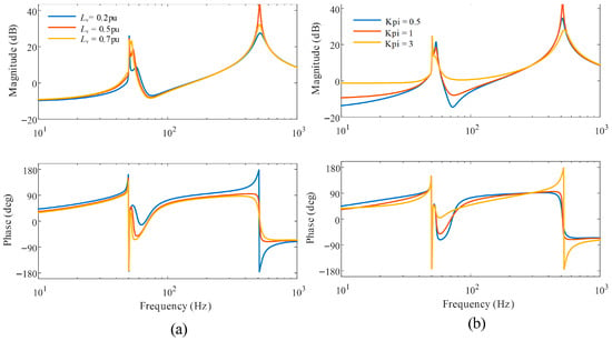
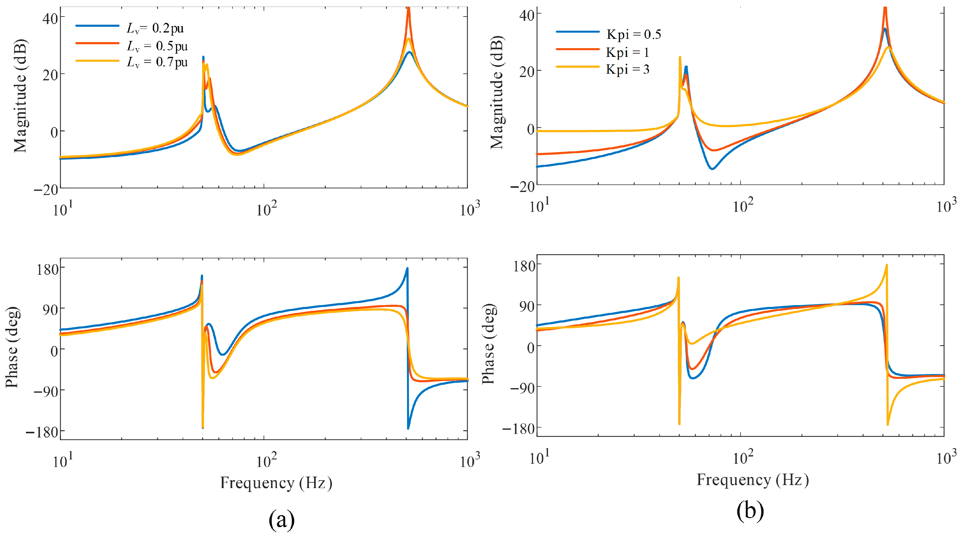
For the VAC structure, a minimum capacity ratio of 75% is required. The virtual inductance Lv and the current-loop proportional gain Kpi exhibit opposing effects on the high-frequency impedance. The impedance curves, as illustrated in Figure 12. Decreasing Lv or increasing Kpi (which generally accelerates the dynamic response)slightly reduces the high-frequency resonance peak but introduces a capacitive negative damping region. As indicated in Figure 7, this negative damping is intrinsically introduced by the GFM inverter itself. Under such parameter settings, the GFM inverter fails to mitigate GFL-induced oscillations and may even provoke new instabilities. To ensure transient stability, Lv is typically constrained between 0.15 pu and 0.3 pu; thus, Lv = 0.3 pu is selected in this study. The impedance curves reveal that setting Kpi avoids the high-frequency negative damping region, whereas an excessively small Kpi deteriorates the sub-synchronous impedance. Hence, Kpi = 1 is selected as the optimal balance.

Figure 12. The influence of VAC parameters on impedance characteristics (a): Virtual inductance; (b): current loop proportional coefficient.

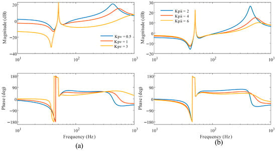
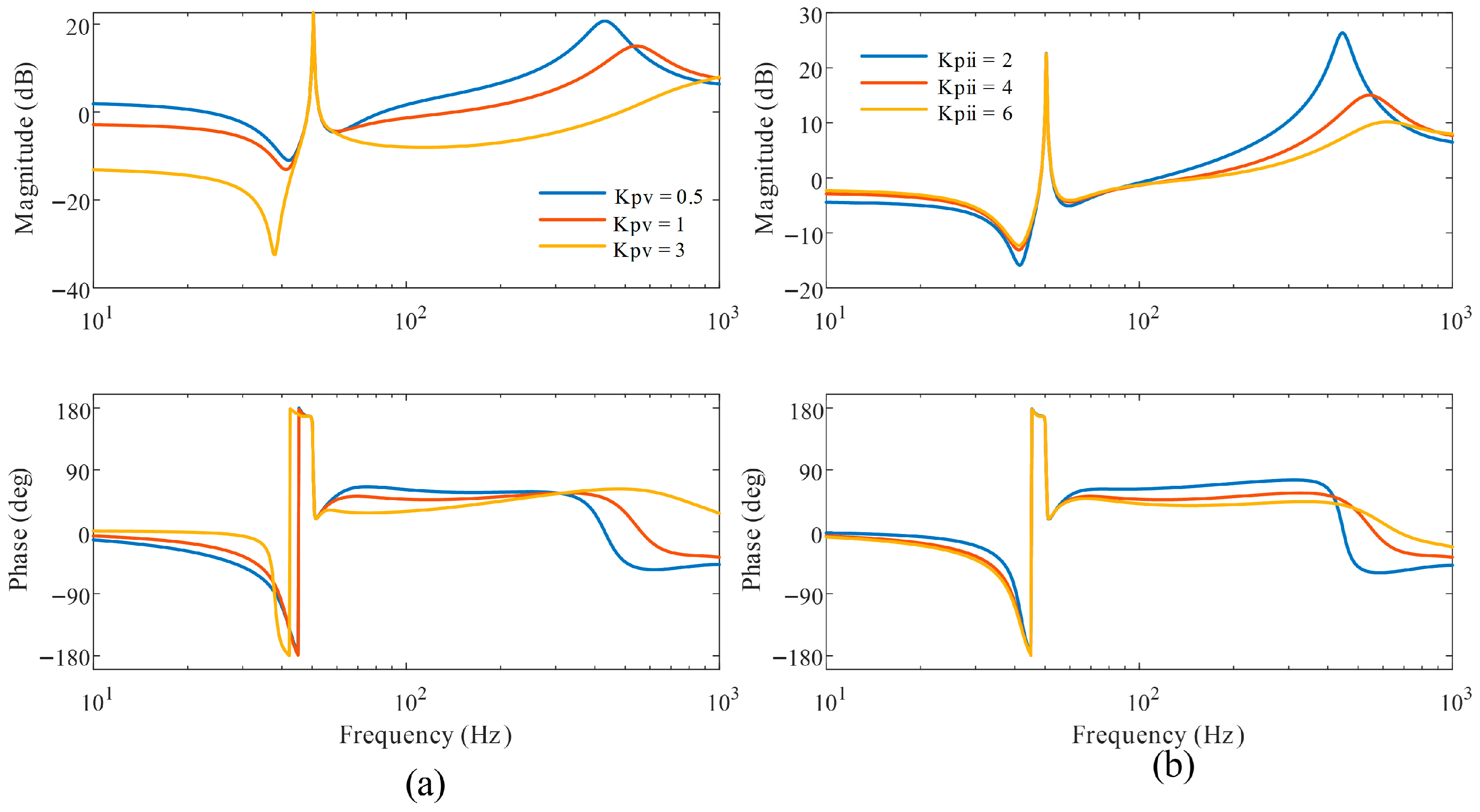
For the DLC structure, the minimum capacity ratio is significantly reduced to 25%. Increasing the proportional gains of both the voltage and current loops yields similar trends: it essentially broadens the control bandwidth (leading to faster dynamic response tracking), while the output impedance magnitude decreases, the high-frequency stability margin improves, and the inductive region expands. However, excessively large parameters in either loop can deteriorate sub-synchronous stability (see Figure 13). Balancing these frequency-domain trade-offs, the DLC parameters are optimized as Kpv = 1 and Kpii = 4.

Figure 13. The influence of DLC parameters on impedance characteristics (a): Proportional coefficient of voltage loop; (b): current loop proportional coefficient.

Combining the analyses from Figure 5 and Figure 6 reveals a fundamental mechanism: increasing the current-loop gain in both structures reduces the GFM inverter’s output impedance magnitude. In a multi-inverter hybrid system, the overall impedance characteristic is dominated by the unit with the lower impedance magnitude. Because the DLC structure does not introduce a mid-to-high-frequency negative damping region, its current-loop gain enjoys a much wider stable tuning range. This allows the DLC to achieve a significantly lower output impedance magnitude, thereby dominating the hybrid system and requiring far less capacity to suppress oscillations.

It should be noted that achieving improved mid-to-high-frequency stability through the DLC structure involves specific control design trade-offs. While increasing the proportional gains of the inner loops effectively mitigates grid-induced high-frequency resonances, it simultaneously broadens the voltage loop bandwidth. This makes it increasingly difficult to maintain a sufficient bandwidth separation between the cascaded voltage and current loops. Consequently, the primary potential cost of this parameter tuning is the heightened risk of dynamic coupling between the inner loops. If the gains are excessively large, this coupling may provoke new internal stability issues, such as sub-synchronous oscillations. Therefore, practical implementation requires a careful compromise between optimizing high-frequency grid interaction damping and preserving the internal cascaded stability margins.

Furthermore, utilizing the open-loop control at a 25% GFM capacity ratio as an illustrative case demonstrates that fluctuations in grid strength significantly alter the stability margins. As the grid strength increases, the intersection point between the grid and hybrid system impedances shifts toward higher frequencies, as shown in Figure 14, progressively enlarging the stability margin.Consequently, a reduced GFM capacity ratio becomes adequate for oscillation suppression in stronger grids. Conversely, although an insufficient GFM capacity may sustain stability under robust grid conditions, subsequent network weakening can readily provoke new resonant instabilities. This inherent sensitivity underscores the critical importance of rigorous architectural selection and precise parameter tuning.

Figure 14. Impact of different grid strengths on system stability.

4. Case Study

4.1. Simulation Setup

To validate the correctness of the theoretical analysis presented above, detailed time-domain simulations are conducted on the MATLAB/Simulink platform. Two simulation scenarios are considered: a single grid-connected GFM inverter system and a hybrid system composed of GFM and GFL inverters. The key system parameters used in the simulations are summarized in Table 1.

4.2. Simulation Results of Single GFM Inverter Connected to the Grid

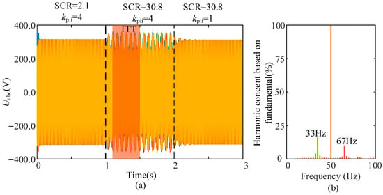
Figure 15 presents the time-domain waveforms and corresponding frequency spectra of the point-of-common-coupling (PCC) voltage for the DLC-based GFM inverter under different control parameters and grid strength conditions.

Figure 15. Grid-connected voltage waveform and spectrum diagram of the DLC. (a) Grid-connected voltage, (b) THD.

Before 1 s, the proportional gain of the inner current loop is set to 4, and the short-circuit ratio (SCR) of the grid is 2.1. Under this condition, the system operates stably. At 1 s, the grid strength is increased to SCR = 30.8 while maintaining the same current-loop gain. As a result, the system becomes unstable, exhibiting oscillatory behavior with dominant frequency components at 33 Hz and an additional coupled component around 67 Hz. At 2 s, the proportional gain of the current loop is reduced to 1 under SCR = 30.8, after which the system remains in stable operation.

The observed dynamic responses are consistent with the impedance-based stability analysis, confirming the validity of the theoretical predictions.

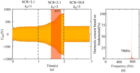
Figure 16 illustrates the PCC voltage waveforms and frequency spectra of the VAC-based GFM inverter under different control parameters and grid strengths.

Figure 16. Grid-connected voltage waveform and spectrum diagram of the VAC. (a) Grid-connected voltage, (b) THD.

Before 1 s, the proportional gain of the current loop is set to 1, and the grid SCR equals 2.1, under which the system operates stably. At 1 s, while maintaining SCR = 2.1, the current-loop proportional gain is increased to 3, leading to oscillatory instability. The dominant oscillation frequency is approximately 780 Hz, as shown in Figure 10b. At 2 s, the grid strength is increased to SCR = 30.8 while keeping the proportional gain unchanged, and the system returns to stable operation.

These simulation results are consistent with the previous stability analysis, further confirming the validity of the proposed impedance modeling approach.

4.3. Simulation Results of Hybrid GFM–GFL Systems

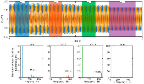
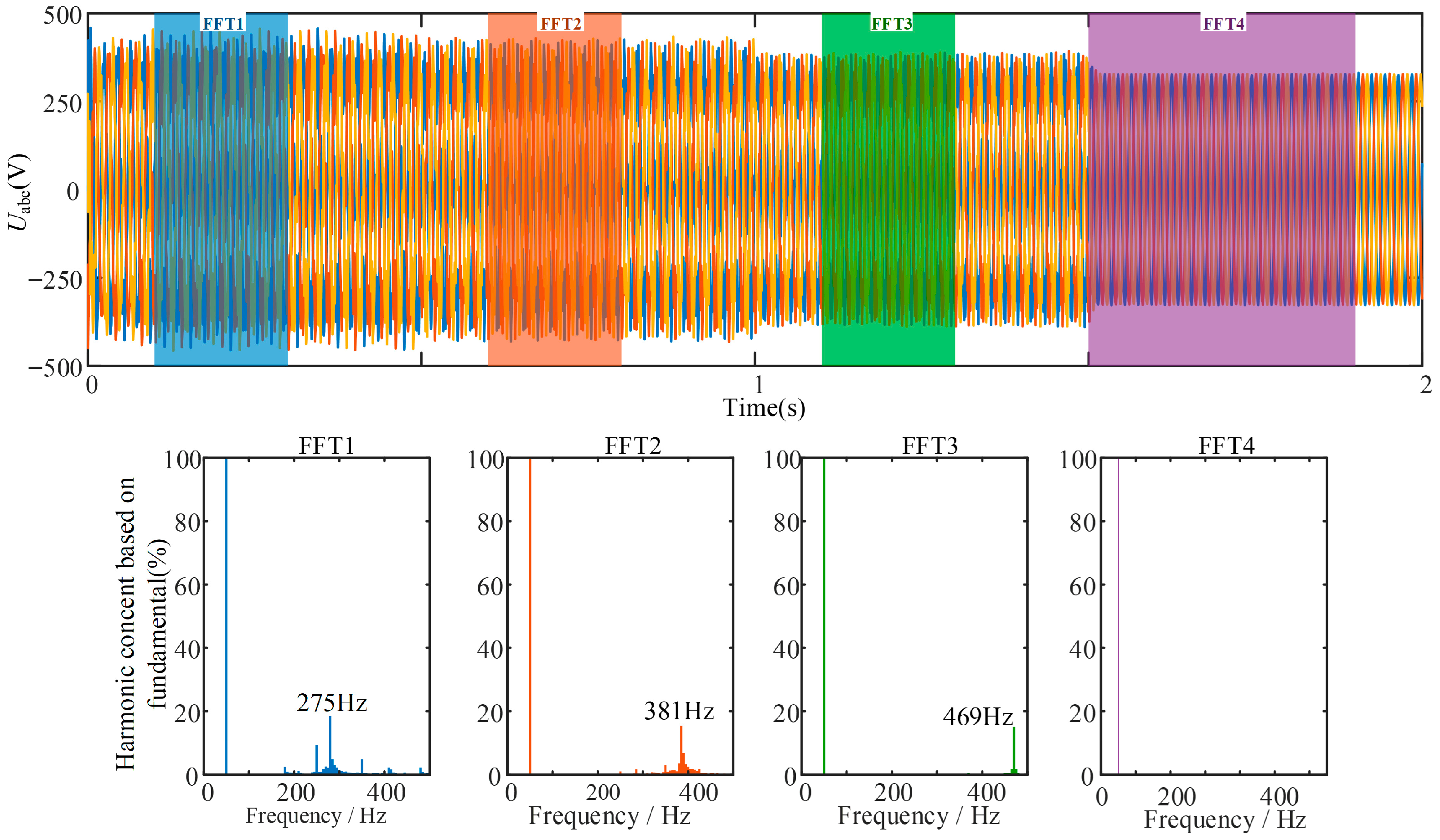
In the hybrid system simulations, the total number of inverters is set to $N=4$, and the grid strength is fixed at SCR = 2.5. During 0–0.5 s, only GFL inverters are connected to the grid. Subsequently, the capacity proportion of GFM inverters is increased to 25%, 50%, and 75% at 0.5 s, 1 s, and 1.5 s, respectively.

Figure 17 shows the PCC voltage waveforms and frequency spectra for the hybrid system composed of VAC-based GFM and GFL inverters. Before 0.5 s, the GFL inverter exhibits medium-frequency oscillations around 275 Hz in the weak grid. When the GFM capacity proportion is increased to 25% at 0.5 s, the oscillation frequency rises to 381 Hz. Further increasing the GFM proportion to 50% at 1 s shifts the oscillation frequency to 469 Hz. When the GFM proportion reaches 75% at 1.5 s, the oscillations are completely suppressed.

Figure 17. Grid-Connected Voltage Waveform and Spectrum Diagram of the VAC Hybrid System.

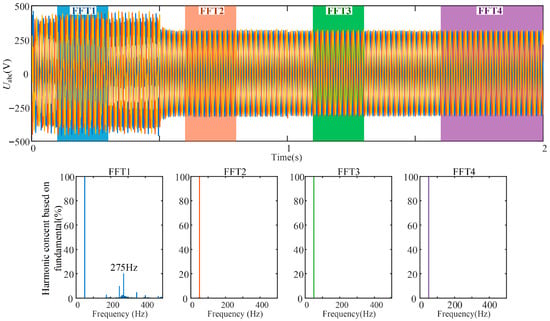
As shown in Figure 18, when DLC-based GFM inverters are introduced into the hybrid system, the medium-frequency oscillations observed in the pure GFL system are completely suppressed once the GFM capacity proportion reaches 25%. Further increasing the GFM proportion to 50% and 75% does not deteriorate system stability.

Figure 18. Grid-Connected Voltage Waveform and Spectrum Diagram of the DLC Hybrid System.

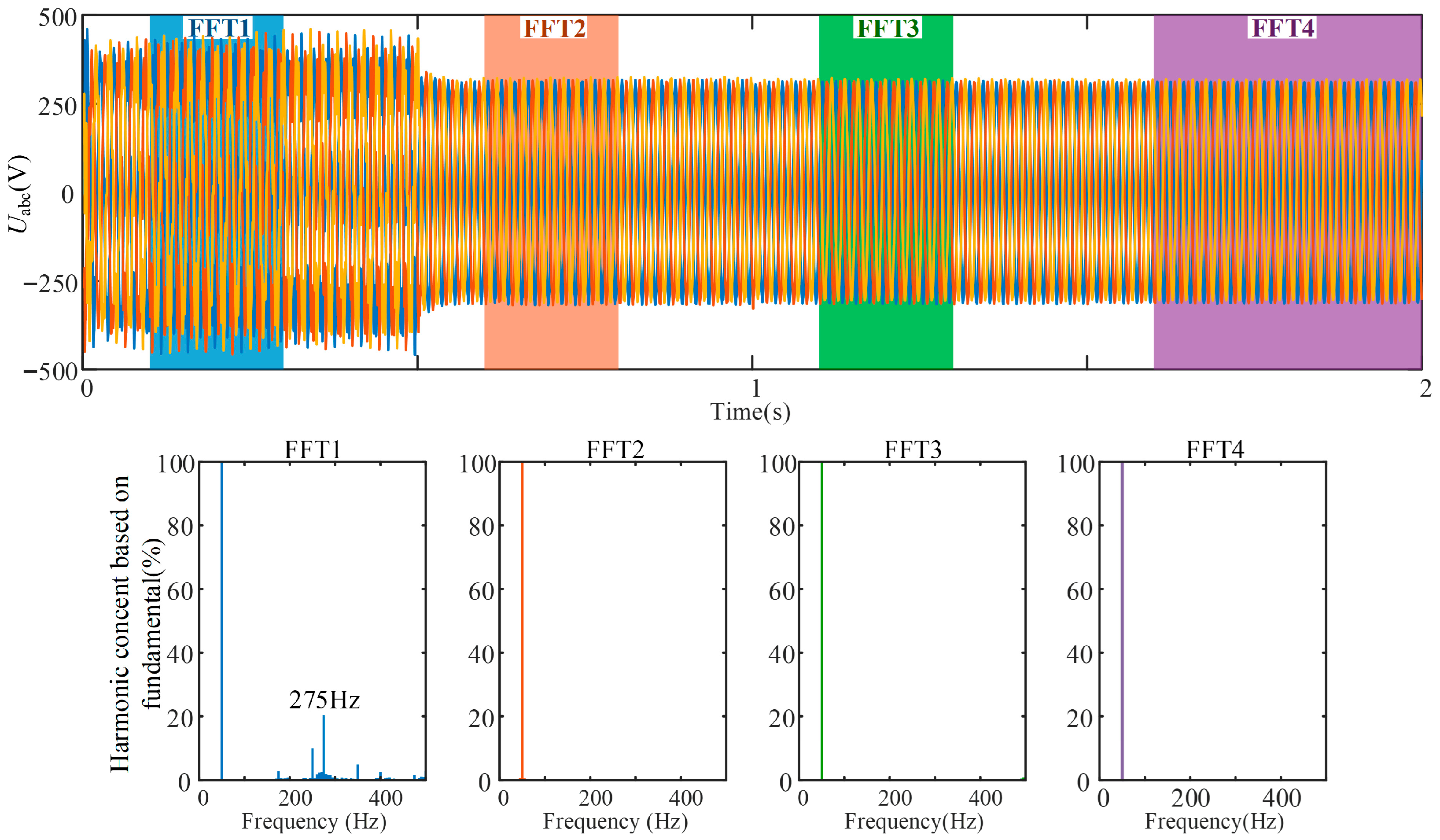
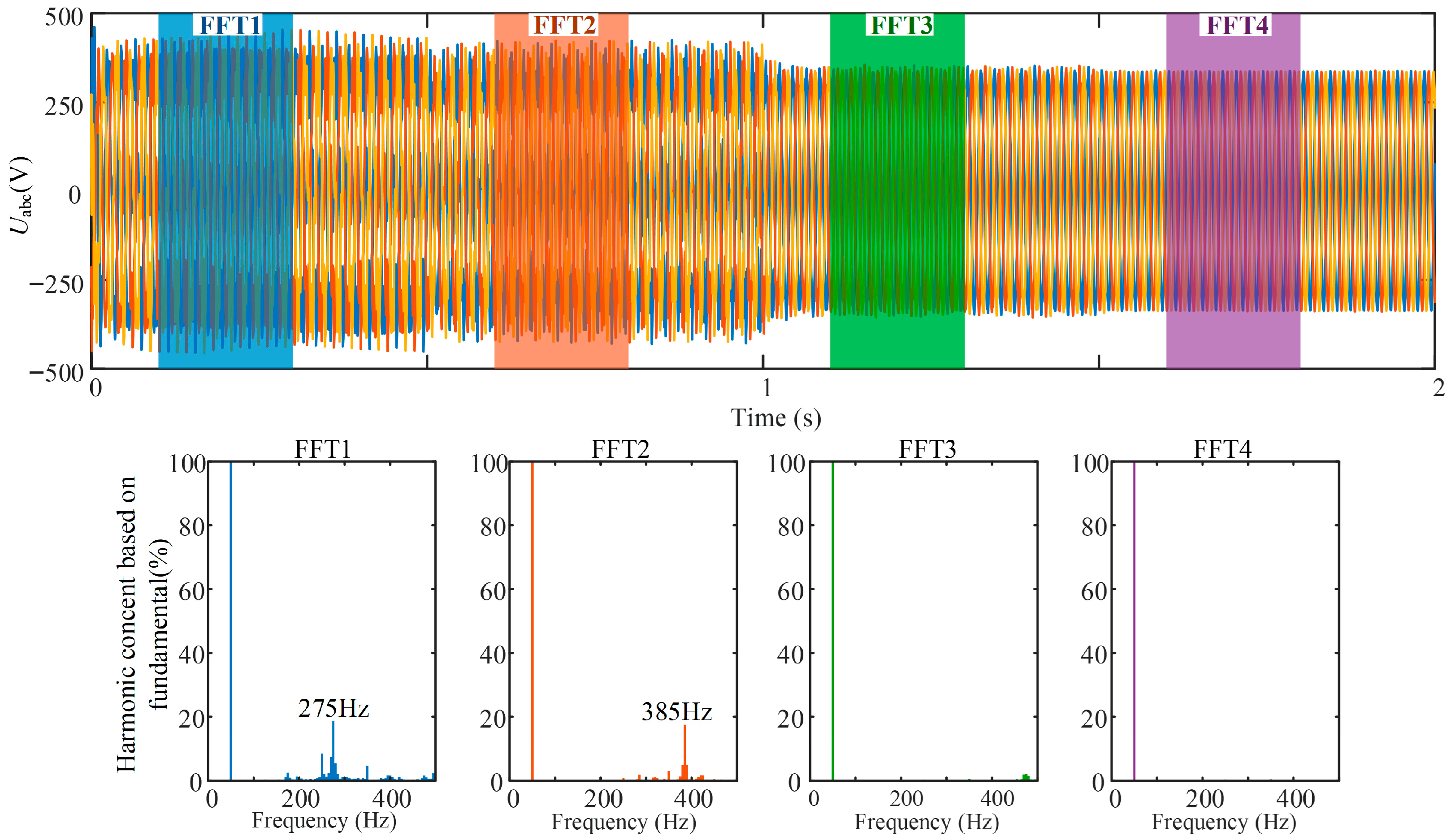
Figure 19 presents the simulation results for the hybrid system composed of open-loop dVOC-based GFM and GFL inverters. Before 0.5 s, oscillations at approximately 275 Hz are observed. At 0.5 s, increasing the GFM capacity proportion to 25% shifts the oscillation frequency to 385 Hz. When the GFM proportion reaches 50% at 1 s, the oscillations are fully eliminated, and the system remains stable as the proportion further increases to 75%.

Figure 19. Grid-Connected Voltage Waveform and Spectrum Diagram of the dVOC Hybrid System.

These results are consistent with the impedance-based stability analysis and demonstrate that the DLC inner-loop structure achieves superior oscillation suppression capability with a significantly lower GFM capacity proportion.

5. Conclusions

This paper establishes sequence impedance models for dispatchable virtual oscillator control (dVOC)-based GFM inverters employing three representative control structures, namely open-loop control, dual-loop DLC, and VAC. Based on the derived models, the stability characteristics of these configurations are systematically investigated in both standalone grid-connected scenarios and hybrid systems comprising grid-forming and grid-following GFM–GFL inverters.

The results indicate that open-loop dVOC control exhibits predominantly inductive impedance characteristics with a relatively simple parameter design, which reduces the likelihood of instability caused by inappropriate tuning. By contrast, the introduction of virtual admittance dynamics in VAC may lead to capacitive negative damping in the medium- and high-frequency ranges, rendering system stability more sensitive to parameter variations. The DLC structure demonstrates strong adaptability to weak grids and preserves inductive impedance characteristics over a wide frequency range.

For hybrid GFM–GFL systems, system stability is shown to be strongly dependent on both the GFM capacity ratio and the adopted control structure. Increasing the proportion of GFM inverters shifts the resonance frequency toward higher ranges and improves phase margin, thereby enhancing overall stability.

Among the investigated control strategies, the DLC-based structure achieves the most favorable balance between stability performance and economic efficiency. Under the specific baseline parameters and grid conditions investigated in this study, stable operation can be ensured with only 25% GFM capacity to suppress the capacitive negative damping introduced by GFL inverters, whereas VAC-based and open-loop dVOC-based configurations require approximately 75% and 50% GFM capacity, respectively. Although sensitivity analyses indicate that these absolute capacity thresholds may vary with changes in grid strength and control parameter tuning, the comparative advantage of the DLC structure remains consistent. These results demonstrate that DLC-based GFM inverters can significantly reduce the required GFM penetration while maintaining system stability, offering superior engineering applicability and economic advantages. Overall, the findings highlight that inner-loop control design constitutes an essential component of grid-forming control strategies and should not be regarded as a secondary implementation detail.

It should be noted that this study focuses on small-signal stability using impedance-based methods. For severe faults such as grid-side voltage drops that may trigger nonlinear converter dynamics, or specific harmonic interferences, the stability analysis would require large-signal or transient modeling. While these aspects are outside the scope of this paper, they represent crucial directions for future research to further enhance the overall robustness of GFM inverters. Further exploration of the integration of advanced control algorithms (such as sliding mode coordinated control) with DLC structures is expected to improve the system’s adaptability to these extreme disturbances while maintaining low GFM capacity requirements.

References

- Ahmadimonfared, Z.; Eichner, S. Stability Assessment of Fully Inverter-Based Power Systems Using Grid-Forming Controls. Electronics 2025, 14, 4202. [Google Scholar] [CrossRef] [Scilit]
- Li, M.; Nian, H. Perturbation Amplitudes Design Method Based on Confidence Interval Evaluation for Impedance Measurement. IEEE Trans. Ind. Electron. 2024, 71, 12323–12337. [Google Scholar] [CrossRef] [Scilit]
- Jiang, K.; Ji, X.; Liu, D.; Zheng, W.; Tian, L.; Chen, S. Small-Signal Modeling of Grid-Forming Wind Turbines in Active Power and DC Voltage Control Timescale. Electronics 2024, 13, 4728. [Google Scholar] [CrossRef] [Scilit]
- Arévalo, P.; Ramos, C.; Rocha, A. A Systematic Review of Grid-Forming Control Techniques for Modern Power Systems and Microgrids. Energies 2025, 18, 3888. [Google Scholar] [CrossRef] [Scilit]
- Dereje, T.; Zhan, L.; Hu, B.; Nian, H. Transient Synchronization Stability Modeling and Analysis of Grid-Following Converter Considering Current Dynamics. IEEE Access 2024, 12, 171066–171075. [Google Scholar] [CrossRef] [Scilit]
- Khan, S.A.; Wang, M.; Su, W.; Liu, G.; Chaturvedi, S. Grid-Forming Converters for Stability Issues in Future Power Grids. Energies 2022, 15, 4937. [Google Scholar] [CrossRef] [Scilit]
- Zhao, F.; Wang, X.; Zhu, T. Power Dynamic Decoupling Control of Grid-Forming Converter in Stiff Grid. IEEE Trans. Power Electron. 2022, 37, 9073–9088. [Google Scholar] [CrossRef] [Scilit]
- Aquib, M.; Parth, N.; Doolla, S.; Chandorkar, M.C. An Adaptive Droop Scheme for Improving Transient and Steady-State Power Sharing among Distributed Generators in Islanded Microgrids. IEEE Trans. Ind. Appl. 2023, 59, 5136–5148. [Google Scholar] [CrossRef] [Scilit]
- Quedan, A.; Wang, W.; Ramasubramanian, D.; Farantatos, E.; Asgarpoor, S. An Adaptive Virtual Oscillator Control Structure for Grid-Forming Inverters. IEEE Syst. J. 2023, 17, 3447–3455. [Google Scholar] [CrossRef] [Scilit]
- Musona, R.; Serban, I. Control of a Single-Phase Islanded Microgrid Based on Virtual Oscillator Control Enhanced with Power Limitation and Robust Distributed Secondary Control. IEEE Open J. Ind. Electron. Soc. 2025, 6, 25–42. [Google Scholar] [CrossRef] [Scilit]
- Liu, J.; Liu, X.; Liu, J.; Li, X.; Wang, J. Adaptive-Droop-Coefficient VSG Control for Cost-Efficient Grid Frequency Support. IEEE Trans. Power Syst. 2024, 39, 6768–6771. [Google Scholar] [CrossRef] [Scilit]
- Xiao, H.; He, H.; Zhang, L.; Liu, T. Adaptive Grid-Synchronization Based Grid-Forming Control for Voltage Source Converters. IEEE Trans. Power Syst. 2024, 39, 4763–4766. [Google Scholar] [CrossRef] [Scilit]
- Rosso, R.; Wang, X.; Liserre, M.; Lu, X.; Engelken, S. Grid-Forming Converters: Control Approaches, Grid-Synchronization, and Future Trends—A Review. IEEE Open J. Ind. Appl. 2021, 2, 93–109. [Google Scholar] [CrossRef] [Scilit]
- Dokus, M.; Mertens, A. Sequence Impedance Characteristics of Grid-Forming Converter Controls. In Proceedings of the 2020 IEEE 11th International Symposium on Power Electronics for Distributed Generation Systems (PEDG); IEEE: Dubrovnik, Croatia, 2020; pp. 413–420. [Google Scholar]
- Yan, S.; Chen, J.; Wang, M.; Yang, Y.; Rodriguez, J.M. A Survey on Model Predictive Control of DFIGs in Wind Energy Conversion Systems. CSEE J. Power Energy Syst. 2024, 10, 1085–1104. [Google Scholar] [CrossRef] [Scilit]
- Zhang, W.; Sun, C.; Alharbi, M.; Hasanien, H.M.; Song, K. A Voltage-Power Self-Coordinated Control System on the Load-Side of Storage and Distributed Generation Inverters in Distribution Grid. Ain Shams Eng. J. 2025, 16, 103480. [Google Scholar] [CrossRef] [Scilit]
- Zhang, W.; Sun, C.; Wang, Y.; Song, K. A Novel Voltage-Power Coordinated Control Strategy for Grid-Connected Inverters in Low-Voltage Microgrids Based on Fast Non-Singular Terminal Sliding Mode. Electr. Power Syst. Res. 2026, 251, 112183. [Google Scholar] [CrossRef] [Scilit]
- Li, Y.; Gu, Y.; Green, T.C. Revisiting Grid-Forming and Grid-Following Inverters: A Duality Theory. IEEE Trans. Power Syst. 2022, 37, 4541–4554. [Google Scholar] [CrossRef] [Scilit]
- Zhang, Y.; Zhang, C.; Yang, R.; Molinas, M.; Cai, X. Current-Constrained Power-Angle Characterization Method for Transient Stability Analysis of Grid-Forming Voltage Source Converters. IEEE Trans. Energy Convers. 2023, 38, 1338–1349. [Google Scholar] [CrossRef] [Scilit]
- Elshenawy, M.A.; Radwan, A.; Mohamed, Y.A.-R.I. Unified Sequence Impedance Models of Synchronous Generator-and Virtual Oscillator-Based Grid-Forming Converters. IEEE Trans. Power Deliv. 2024, 39, 56–70. [Google Scholar] [CrossRef] [Scilit]
- Zhao, L.; Wang, X.; Jin, Z. Exploring Damping Effect of Inner Control Loops for Grid-Forming VSCs. IEEE Open J. Power Electron. 2025, 6, 1595–1608. [Google Scholar] [CrossRef] [Scilit]
- Liu, J.; Xia, Y.; Wei, W.; Feng, Q.; Yang, P. Effect of Control Damping on Small-Signal Stability of Grid-Forming VSCs Considering Interaction Between Inner and Outer Loops. IEEE Trans. Power Electron. 2024, 39, 7685–7695. [Google Scholar] [CrossRef] [Scilit]
- Xin, H.; Liu, C.; Chen, X.; Wang, Y.; Prieto-Araujo, E.; Huang, L. How Many Grid-Forming Converters Do We Need? A Perspective from Small Signal Stability and Power Grid Strength. IEEE Trans. Power Syst. 2025, 40, 623–635. [Google Scholar] [CrossRef] [Scilit]
- Sun, P.; Xu, H.; Yao, J.; Chi, Y.; Huang, S.; Cao, J. Dynamic Interaction Analysis and Damping Control Strategy of Hybrid System with Grid-Forming and Grid-Following Control Modes. IEEE Trans. Energy Convers. 2023, 38, 1639–1649. [Google Scholar] [CrossRef] [Scilit]
- Chi, S.; Zhang, R.; Chen, A.; Cheng, C.; Sun, S.; Yu, P.; Cheng, Y. Interaction Stability Analysis and Oscillation Suppression Method of Hybrid Grid-Forming and Grid-Following Inverters System with Varying Power Levels. IEEE Trans. Ind. Electron. 2026, 73, 755–766. [Google Scholar] [CrossRef] [Scilit]
- Xiong, X.; Zhou, Y.; Luo, B.; Cheng, P.; Blaabjerg, F. Analysis and Suppression Strategy of Synchronous Frequency Resonance for Grid-Connected Converters with Power-Synchronous Control Method. IEEE Trans. Power Electron. 2023, 38, 6945–6955. [Google Scholar] [CrossRef] [Scilit]
- Wu, W.; Zhou, L.; Chen, Y.; Luo, A.; Dong, Y.; Zhou, X.; Xu, Q.; Yang, L.; Guerrero, J.M. Sequence-Impedance-Based Stability Comparison Between VSGs and Traditional Grid-Connected Inverters. IEEE Trans. Power Electron. 2019, 34, 46–52. [Google Scholar] [CrossRef] [Scilit]
- Mu, T.; Duan, J.; Yang, Z.; Wang, H.; Pei, H.; Zhao, K. Mid-Frequency Oscillation Analysis and Suppression in Grid-Following Renewable Energy and Gridforming Energy Storage Hybrid Systems. In Proceedings of the 2025 IEEE 16th International Symposium on Power Electronics for Distributed Generation Systems (PEDG); IEEE: Nanjing, China, 2025; pp. 765–770. [Google Scholar]
Disclaimer/Publisher’s Note: The statements, opinions and data contained in all publications are solely those of the individual author(s) and contributor(s) and not of MDPI and/or the editor(s). MDPI and/or the editor(s) disclaim responsibility for any injury to people or property resulting from any ideas, methods, instructions or products referred to in the content. |
© 2026 by the authors. Licensee MDPI, Basel, Switzerland. This article is an open access article distributed under the terms and conditions of the Creative Commons Attribution (CC BY) license.