


Abstract
Reported forced outages may provide forecast-relevant information for short-term power generation forecasting. This study examines whether their predictive contribution in spatio-temporal Graph Neural Networks (GNNs) can be distinguished from the generic effect of adding an input channel. Hourly ENTSO-E data for Poland were evaluated over 12 quarters of 2022–2024 using a rolling-origin design, eight random seeds per quarter, and four architectures. A surrogate-controlled design decomposed the conventional ablation contrast into an information component and a channel component. The pooled information component was 0.77 MW (95% confidence interval [−0.60, 2.15]), while the channel component was −1.52 MW (95% confidence interval [−3.16, 0.11]); both varied substantially across quarters. Under matched information and equal tuning, no graph architecture differed significantly from the non-graph Temporal Fusion Transformer. However, because the original publication times of outage messages could not be reconstructed, the results do not establish that outage information was available at the corresponding forecast origins or that it provides predictive value in real time. The study evaluates forecast accuracy only; operational effects are not assessed.
1. Introduction
The energy sector is a core component of national economies and influences the performance of other economic sectors [1,2]. In this sector, there is an ongoing transition from fossil fuels towards renewable energy sources, driven in the European Union by the Fit for 55 legislative package [3] and by the REPowerEU Plan [4]. The growing share of non-dispatchable generation increases the complexity of system balancing and imposes higher requirements on short-term generation forecasting performed by transmission system operators (TSOs) [5,6]. Between 2021 and 2024, the share of wind and solar generation in the mean generation of the Polish power system increased from 12.3% to 26.5% [7].
The forecasting task becomes particularly demanding during forced outages of conventional generation units. Forced outages are unplanned events, and information on them is disclosed under Regulation (EU) No. 1227/2011 on wholesale energy market integrity and transparency (REMIT) [8] and published through the ENTSO-E Transparency Platform [7]. The analysis of these data for the Polish bidding zone in 2023 indicates that in 98.2% of all hours (8601 out of 8760), at least one generation unit had an unavailable capacity of at least 100 MW due to a forced outage. Hard coal, which contributed 42.6% of the mean system generation, accumulated 8472 h with at least one active forced outage. Large generation losses can alter the short-term balance between generation and demand. Consequently, information on forced outages may provide an additional input for short-term generation forecasting over the 1–24 h horizon.
Graph Neural Networks (GNNs) have become widely used for forecasting spatially structured time series [9,10] and have been applied in the energy domain to power system load forecasting [11,12] and to short-term wind speed forecasting [13]. Architectures such as the Diffusion Convolutional Recurrent Neural Network (DCRNN) [9] and Graph WaveNet [10,14] exploit spatial dependencies between interconnected or related time series, while their graph structures are typically derived from historical relationships, geographical information, or learned representations [15,16].
This raises a more specific question for power generation forecasting: whether operational events reported in near-real time, such as forced outages, contain predictive information that is not captured by the historical spatial structure alone. Although forced outages are explicitly reported through electricity market transparency mechanisms, their predictive value for short-term generation forecasting with spatio-temporal GNNs remains insufficiently established. In particular, it is necessary to distinguish a genuine contribution of the reported outage information from an apparent improvement caused simply by providing an additional input channel.
Conventional feature-ablation designs do not fully resolve this problem. Comparing a model with an additional variable against a model without that variable establishes whether the augmented specification performs differently, but it does not determine whether the observed difference is attributable to the information encoded in the added variable. An additional channel may itself affect model optimisation, regularisation, or sensitivity to random initialisation, even when the channel contains no information relevant to the forecasting target. A stricter evaluation therefore requires a control that preserves the statistical characteristics of the additional channel while disrupting the temporal relationship that could make the channel predictive. This distinction is particularly relevant for operational event data, because reported outages are temporally structured, strongly autocorrelated, and heterogeneous across generation types. A statistically matched surrogate can therefore provide a more demanding counterfactual than conventional feature ablation: it retains the burden of processing an additional channel while removing its temporal alignment with the forecasting target.
The attribution of predictive content to individual inputs is addressed by several families of methods. Permutation importance measures the increase in the error of a fitted model when the values of one input are permuted [17,18] and its conditional variants restrict the permutation to preserve the dependence between inputs [19]. Because the model is not retrained, a permuted input can force the model to extrapolate outside the training distribution [20]. Leave-one-covariate-out designs retrain the model without the tested input [21], and the remove-and-retrain benchmark replaces the most important inputs with uninformative values before retraining [22]. Model-X knockoffs and shadow features add synthetic or permuted copies of the inputs as a reference for variable selection [23,24]. The closest design to the one adopted here replaces the tested inputs with permuted copies and retrains the model, so that both compared models receive inputs of the same dimension [25]. On the other hand, a permuted copy does not preserve the temporal dependence of a time series, and the method of surrogate data was developed to construct null series that preserve selected properties of an observed series while destroying the property under test [26,27]. Reported forced outages are strongly autocorrelated and covary across production types, therefore a copy that destroys this structure differs from the reported series in more than its alignment with generation. Finally, there is a research gap related to the attribution of the predictive content of temporally structured operational event series in stochastic spatio-temporal forecasting models, and this paper covers this research gap with a retraining design based on structure-preserving surrogates.
The aim of this study is to determine whether reported forced outages provide predictive information for short-term power generation forecasting with spatio-temporal models and to identify the conditions under which this information contributes to forecasting performance, with a focus on distinguishing information-specific effects from the generic impact of adding an additional input channel. The analysis focuses on an exogenous outage channel representing the magnitude of lost generation capacity and evaluates its contribution through controlled ablation and surrogate experiments. Hourly generation and forced-outage data for the Polish bidding zone from November 2020 to December 2024 are analysed in a rolling-origin evaluation over twelve quarters with Graph WaveNet as a primary architecture and the seasonal naive as a reference. The DCRNN and STCN and the Temporal Fusion Transformer added on six of these quarters, the first and third quarter of each year. Paired random seeds, Deep Ensembles, moving-block bootstrap inference, a random-effects meta-analysis across folds, and surrogate outage series are used to distinguish the contribution of temporally aligned outage information from variation associated with model initialization and the addition of an arbitrary input channel. The study therefore treats forced outages primarily as an exogenous information channel and tests whether their predictive contribution arises from the temporal alignment of reported capacity losses with generation rather than from a change in graph topology.
2. Materials and Methods
2.1. Research Design
The research procedure adopted in this paper is a controlled computational experiment in which the manipulated factor is the content of an exogenous forced-outage input channel: no channel, the reported outage series, or a surrogate of that series [9,10]. The experiment is replicated over rolling forecast origins covering three calendar years and over paired random seeds, which are the two levels at which the treatment is repeated [28,29]. All compared architectures receive the same input information and the same hyperparameter-search budget, so that the comparison between architectures is not confounded with tuning effort or with the input specification. The primary contrast, the reported outage series against the rotated surrogate for Graph WaveNet in the Polish bidding zone, was declared before the evaluation. The remaining contrasts form a secondary family with a family-wise error correction.
The research questions and the corresponding hypotheses are formulated in Table 1.
Table 1.
Research questions and hypotheses.
2.2. Data Source and Scope
All data used in this study were obtained from the ENTSO-E Transparency Platform [7], which is the official public repository of European electricity market data. The platform operates under Commission Regulation (EU) No. 543/2013 [30] on submission and publication of data in electricity markets, and the outage messages published there are disclosed in accordance with Regulation (EU) No. 1227/2011 on wholesale energy market integrity and transparency (REMIT) [8]. Therefore, the data are public, standardised across bidding zones, and legally mandated, which supports the reproducibility of the presented procedure.
Three datasets were downloaded through the application programming interface of the platform. The first dataset is Actual Generation per Production Type, expressed in MW. The second dataset is Unavailability of Production and Generation Units, published as Urgent Market Messages under REMIT. The third dataset is Installed Capacity per Production Type, which provides the denominator of the outage channel (Section 2.6). The scope of the acquired data is presented in Table 2.
Table 2.
Scope of the acquired data.
The Polish bidding zone was selected for three reasons. Firstly, the generation mix of this zone remains dominated by conventional thermal units, which are the units subject to forced outages of large magnitude. Secondly, the zone is operated as a single bidding zone, therefore the published generation aggregates refer to one consistent market area. Thirdly, the platform publishes complete generation series for this zone over 2020–2024, which allows twelve consecutive quarters to be evaluated, each with a training period covering a full annual cycle.
The test quarters cover the years 2022–2024 (Section 2.10), therefore the training period of the first fold starts in November 2020. The Polish zone reports generation at hourly resolution until mid-2024 and at 15 min resolution afterwards; the 15 min values were averaged to hours.
2.3. Nodes of the Spatio-Temporal Graph
Each electricity production type reported by the platform throughout the period constitutes one node of the graph, which yields N = 11 nodes, and the node set is the same in all folds. The types “Other” and “Other renewable”, which the platform reports for the Polish zone only from mid-2024, were excluded, because in every earlier fold they would enter the model as series of zeros. The descriptive statistics of the nodes are presented in Table 3. The generation mix is dominated by two fossil nodes, Fossil Hard coal and Fossil Brown coal/Lignite, which jointly contribute 67.5% of the mean system generation. The highest relative variability is observed for Solar, which is consistent with the non-dispatchable character of this source [5,6], and for Hydro Pumped Storage, which generates only in selected hours.
Table 3.
Descriptive statistics of the graph nodes, PL bidding zone, 1 November 2020–31 December 2024.
2.4. Forced Outage Events
The raw unavailability messages contain both planned maintenance and unplanned events. The messages were filtered in four steps. Firstly, only the messages describing unplanned or forced unavailability were retained, and the messages with the status cancelled or withdrawn were removed. Secondly, the unavailable capacity of each message was computed as the difference between the nominal capacity of the unit and the capacity available during the event. Thirdly, only the messages with an unavailable capacity of at least 100 MW were retained; the threshold removes events of small magnitude from the analysis. Fourthly, overlapping messages concerning the same generation unit were merged by taking, for every hour, the largest unavailable capacity reported for that unit.
The filtered events were subsequently expanded into an hourly matrix of unavailable capacity, denoted as L ∈ ℝT×N, where the element Lt,i is the total unavailable capacity of node i in hour t. A forced-outage event is a message retained after the filtering; a message is active in hour t if its start precedes or coincides with t and its end follows t.
The unavailable capacities of the units of one production type were then summed. The resulting outage statistics for each year of the period are presented in Table 4.
Table 4.
Forced outages of at least 100 MW of unavailable capacity, PL bidding zone.
In every year of the period, at least one node experienced an active forced outage in more than 98% of hours (Table 4). Consequently, the outage channel is a persistent exogenous input rather than an indicator of rare events.
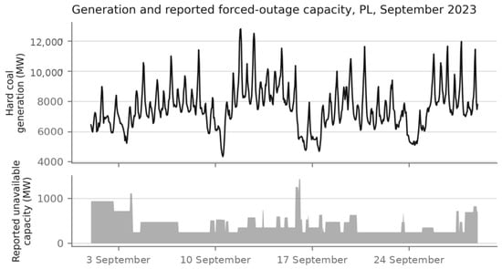
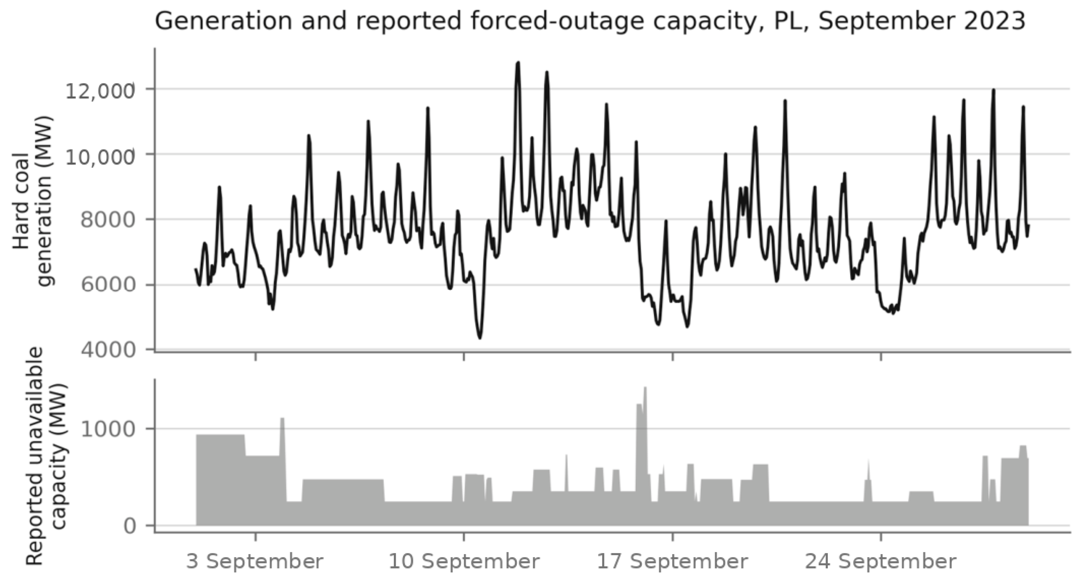
An illustrative month of the raw material is presented in Figure 1, which juxtaposes the generation of the most outage-exposed node with the system-wide reported unavailable capacity.
Figure 1.
Generation and reported forced-outage capacity, PL bidding zone, September 2023. Source: Own elaboration based on ENTSO-E data.
2.5. Construction of the Base Adjacency Matrix
The base adjacency matrix Abase ∈ ℝN×N is constructed from the statistical dependence between the generation time series, because the production types do not possess a physical interconnection topology comparable with the road networks or the sensor networks for which the applied architectures were originally proposed [9,31]. The construction procedure consists of four steps.
Firstly, the pairwise absolute Pearson correlation coefficient |ρij| is computed between the generation series of every pair of nodes separately in each fold, on the training period of that fold only, so that neither the validation nor the test period enters the graph. Secondly, for each node i the k = 4 most correlated neighbours are selected, which yields a directed k-Nearest Neighbours (kNNs) graph. Thirdly, the matrix is symmetrised as A = max(A,AT). Fourthly, self-loops are added, so that Aii = 1 for every node i.
The value k = 4 was selected because the empirically observed dependence structure is concentrated in a small number of strong relations. In the training periods of the twelve folds, the absolute correlation between Fossil Hard coal and Fossil Brown coal/Lignite ranged from 0.57 to 0.76, and that between Fossil Gas and Fossil Hard coal from 0.30 to 0.62.
2.6. Input Specifications
The outage information is supplied as an additional input channel containing the unavailable capacity of a node normalised by the installed capacity of the corresponding production type, that is. The installed capacity is the value published by the platform for the year in which the test period of the fold begins, which is known before the first forecast of that period; where the platform publishes no value, the maximum generation of the training period is used Lt,i/Ci. Normalisation makes the channel comparable across production types of substantially different sizes.
Three input specifications are compared: no outage channel, the reported outage channel, and a surrogate of the outage channel (Section 2.7). The graph structure is the same static base adjacency matrix in all three. A per-step masking of the edges incident to nodes with an active outage, which was considered in the initial design of the study, was not executed and is not evaluated in this paper.
2.7. Surrogate-Controlled Attribution
Three input specifications are compared under an identical architecture, hyperparameter configuration, fold and set of random seeds. The first specification receives no outage channel, the second receives the reported outage series, and the third receives a surrogate of the reported series. The expected test errors of the three specifications are denoted L(∅), L(X) and L(), where the expectation is taken over the random initialisation of the trained model [29].
The conventional feature-ablation contrast is Δabl = L(∅) − L(X), and it decomposes exactly into two components, Δabl = Δinfo + Δch, where Δinfo = L() − L(X) and Δch = L(∅) − L().
The component Δinfo compares two models that receive inputs of the same dimension, scale, marginal distribution and temporal dependence, and that differ only in the property destroyed by the surrogate. The component Δch measures the effect of supplying an additional channel that carries no information about that property. An uninformative channel is not neutral for a stochastic deep learning model, because it changes the parameterisation of the input layer, the optimisation path and the dispersion of the trained models across initialisations [29,32]. Consequently, a conventional ablation contrast close to zero is compatible with a positive information component offset by a negative channel component, and a positive ablation contrast is compatible with a positive channel component and no information at all. The decomposition identifies Δinfo only to the extent that the surrogate preserves every property of the reported series except the one under test; the construction of the surrogate follows this requirement.
The surrogate is a circular shift in the complete outage series of a fold by an offset drawn independently for each random seed. The rotation preserves the marginal distribution of the unavailable capacity exactly, the autocorrelation of every node series, and the covariation between nodes, and it destroys only the temporal alignment between the outages and the generation [26,27]. The offset is bounded away from zero and from the length of the series by 15% of that length. Because every fold is longer than one year, offsets within 14 days of a whole number of years are redrawn, as such an offset would restore the seasonal alignment of the outages with the generation. Table 5 positions the adopted design against the conventional alternatives.
Table 5.
Designs for attributing predictive content to an input channel.
The contribution of this design is therefore not a new principle of variable importance. It combines the equal-dimension replacement of [25] with a surrogate that preserves the temporal structure of an operational event series [26,27], and it estimates both components of the ablation contrast with paired random seeds across rolling forecast origins. To the knowledge of the authors, retraining with a structure-preserving temporal surrogate of an exogenous event channel has not been used to evaluate spatio-temporal forecasting models. The p-values reported in this paper are not derived from the distribution of the surrogates, whose circular-shift construction does not yield exact tests [33]. They are derived from the block bootstrap over forecast origins and from the mixed model over folds and seeds described in Section 2.12.
2.8. Input Features
Each node in each time step is described by a vector of six exogenous features, which are specified in Table 6. The temporal covariates are encoded with sine and cosine transformations, which preserve the cyclical continuity of the hour and of the day of the year. In the specification without the outage channel, the first feature is removed and the model receives five features. All models, including the non-graph reference, receive the same input information: 48 h of history of the target series, the five calendar channels and, in the specifications with outage information, the outage channel of the node. The calendar channels are computed in Coordinated Universal Time.
Table 6.
Input features of a single node.
2.9. Forecasting Models
Three GNN architectures and two references were examined. The GNN architectures represent three families of spatio-temporal modelling: the recurrent family, the convolutional family with an adaptive adjacency matrix, and the convolutional family without it. Every architecture received the same hyperparameter-search budget and the same input information (Section 2.8 and Section 2.11), so that the differences between architectures are not confounded with tuning effort or with the input specification.
The Diffusion Convolutional Recurrent Neural Network (DCRNN) [9] represents the spatial dependence as a bidirectional diffusion process, that is a truncated random walk on the graph, and it combines this operator with Gated Recurrent Unit hidden states.
Graph WaveNet is the primary architecture [14]. It combines dilated causal convolutions in the temporal dimension with a graph convolution that uses both the supplied adjacency matrix and an adaptive adjacency matrix learned from node embeddings.
The Spatio-Temporal Convolutional Network (STCN) is the implementation of [31] the Torch Spatiotemporal library [34], which interleaves temporal convolutions with diffusion graph convolutions. It does not contain any adaptive adjacency mechanism; therefore, it depends entirely on the supplied graph.
The Temporal Fusion Transformer (TFT) is the non-graph deep learning reference [35]. The model applies variable selection networks and multi-head temporal attention. It is a global model with weights shared across the node series, and it does not exploit the inter-node structure. It receives the calendar channels and the outage channel of each node as historical exogenous inputs, and it is early-stopped on the same validation period as the graph models with the step-based rule given in Table 7.
Table 7.
Training configuration.
The seasonal naive model constitutes the lower bound. The forecast for hour t is equal to the observed generation in hour t − 24, which corresponds to one diurnal cycle. This baseline requires no training and is a standard reference in the forecasting literature [36]. The hyperparameters selected by the search described in Section 2.11 and the numbers of trainable parameters are presented in Table 8.
Table 8.
Selected hyperparameters and trainable parameters (without/with the outage channel).
2.10. Rolling-Origin Evaluation
The evaluation uses rolling forecast origins, which replace a single chronological split with a sequence of forecast origins and is the recommended design for time series whose properties change over time [28,37]. Each fold consists of a training period of 12 months, a validation period of 2 months directly preceding the test period, and a test period of one calendar quarter. The test periods are the 12 quarters from the first quarter of 2022 to the fourth quarter of 2024. They include the supply disturbances of 2022, to which the REPowerEU Plan responded [4], and three consecutive years of changes in the installed capacity of the Polish system, in which the installed capacity of hard coal units decreased from 20,925 MW to 18,831 MW and that of gas units increased from 2555 MW to 5162 MW between the 2021 and 2024 publications of the platform [7]. The fold calendar is presented in Table 9.
Table 9.
Folds of the rolling-origin evaluation.
A forecasting window belongs to a period only if its whole 24 h horizon lies inside that period; therefore no training target reaches into the validation period and no validation target into the test period, whereas the 48 h input window of a validation or test forecast may contain earlier observations, as it would in operation. The base adjacency matrix, the target scaling and the outage denominators are computed from information available before the test period of each fold.
2.11. Hyperparameter Search and Training Configuration
Every architecture received the same hyperparameter-search budget: 30 trials of the Tree-structured Parzen Estimator implemented in Optuna [38], and the same objective, the validation MAE in MW on the validation period of the first fold. The graph models were trained with the same maximum number of epochs and the same early-stopping rule, and their unpromising trials were stopped by median pruning. TFT implemented in NeuralForecast is trained in optimization steps rather than epochs, and its trails were run to completion (Table 7, Appendix A). The search used only the training and validation periods of the first fold, so that no test period entered the selection, and it was conducted on the specification without the outage channel, so that the selected configuration does not favour the outage channel. The search spaces are listed in Appendix A. The selected configuration of each architecture was then used without change in every fold and specification, with the training settings presented in Table 7. The target variable was standardised, and the reported errors were transformed back to the original unit of MW before evaluation.
2.12. Evaluation Metrics and Statistical Inference
The forecasts were evaluated on the test period of every fold with the metrics presented in Table 10. The MAE is the primary evaluation metric because it is expressed in MW, the unit of the forecast target. The Root Mean Squared Error (RMSE) is reported as a complementary metric, because it penalises large individual errors more strongly and is consequently informative for the periods of abrupt generation change. The horizon-resolved MAE is computed separately for each step of the forecast horizon in order to describe the degradation of accuracy with the increasing lead time.
Table 10.
Evaluation metrics.
Inference proceeds at three levels [16,39]. Within each fold, the ensemble of all trained seeds of a specification (eight in the primary block, five in the comparison of architectures) is evaluated on the test period, and the difference between two specifications is tested with a moving-block bootstrap over forecast origins, with a block length of 48 h and 2000 replications, applied to the paired difference in the absolute errors; adjacent origins overlap in 23 of the 24 h of the horizon, therefore the errors of single origins are not independent. Across folds, the fold estimates are pooled with a random-effects meta-analysis [40], which yields a pooled difference with a 95% confidence interval and a 95% prediction interval for the difference expected in a new quarter; the prediction interval is the direct measure of robustness across operating regimes. At the level of the random seed, the paired differences in single-model errors in every fold and seed enter a linear mixed model with a random intercept for the fold [41,42]. The number of paired differences is the product of the numbers of folds and seeds.
The primary contrast is tested at the 5% level without adjustment [29]. The secondary family consists of five contrasts: the conventional ablation contrast and the channel contrast of Graph WaveNet, and the ablation contrasts of DCRNN, STCN and TFT; its family-wise error rate is controlled with the Holm procedure [43]. The comparison of architectures under matched information is reported descriptively, as fold-level and pooled differences against TFT, and every other analysis is reported as exploratory [43,44].
2.13. Experimental Matrix
The experiments are enumerated in Table 11. The primary block replicates the three input specifications of Graph WaveNet over all twelve folds with eight random seeds. The comparison of architectures under matched information covers DCRNN, STCN and TFT with and without the outage channel on every other fold, that is on the first and third quarters of each year (2022Q1 up to 2024Q3) with five random seeds. Graph WaveNet enters this comparison with its primary-block runs of the same folds and seeds.
Table 11.
Matrix of the experiments.
2.14. Tools, Environment, and Reproducibility
The complete pipeline was implemented in Python 3.10. The components of the software environment are presented in Table 12. The environment is declared in a lockfile managed by the pixi package manager, the experiment configuration is declared in Hydra configuration groups, and every training run stores its configuration, its metrics and its test predictions in a separate record file. The hyperparameter search is recorded in an Optuna study database. These records were used to compute every reported number, and they support the reproducibility of the analysis.
Table 12.
Software environment.
3. Results
3.1. Information and Channel Components Across Folds
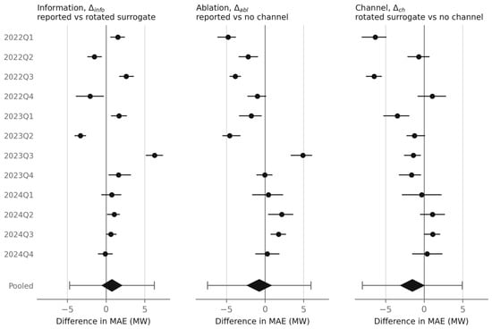
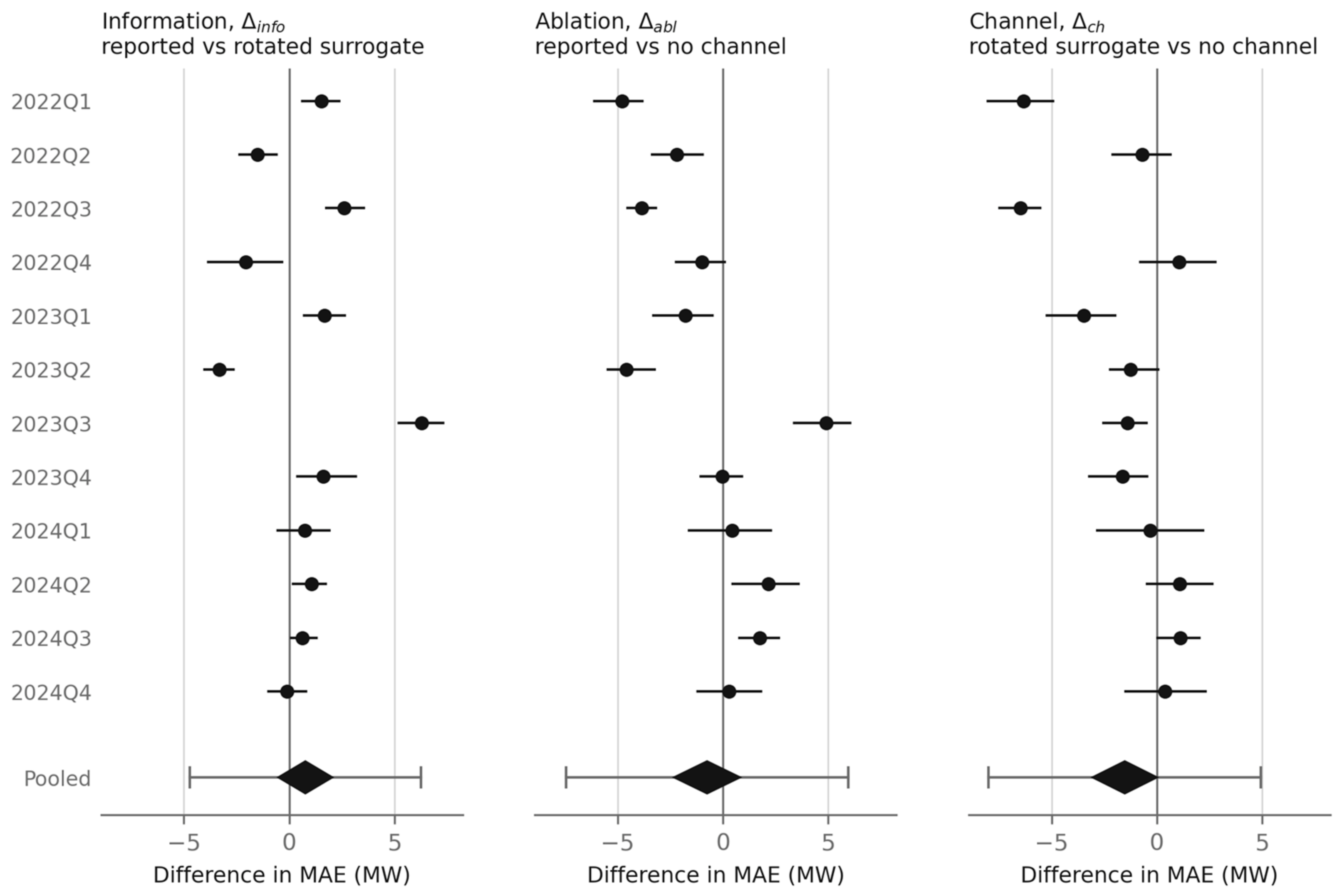
The contrasts between the three input specifications of Graph WaveNet are presented in Table 13 and, for each fold, in Figure 2. Pooled over the 12 folds, the information component, that is the difference between the MAE of the configuration receiving the rotated surrogate and that of the configuration receiving the reported outage series, is 0.77 MW, with a 95% confidence interval of [−0.60, 2.15] MW (p = 0.270). The conventional ablation contrast is −0.76 MW [−2.43, 0.92], and the channel component is −1.52 MW [−3.16, 0.11]. The pooled estimates satisfy the decomposition of Section 2.7 up to rounding.
Table 13.
Information, ablation and channel contrasts, Graph WaveNet, PL bidding zone, 12 folds. A positive difference indicates that the first-named specification is more accurate.
Figure 2.
Information, ablation and channel contrasts by fold, Graph WaveNet, PL bidding zone. Points denote fold estimates with 95% moving-block bootstrap intervals, diamonds the pooled random-effects estimates with 95% confidence intervals, and whiskers the 95% prediction intervals for a new quarter. A positive difference indicates that the first-named specification is more accurate. Source: Authors’ elaboration.
The pooled estimates conceal a strong heterogeneity across operating periods. For all three contrasts, the I2 statistic exceeds 94%, that is, the variation in the fold estimates is dominated by differences between the folds rather than by sampling error, and the 95% prediction interval for the effect expected in a new quarter ranges from −4.73 to 6.27 MW for the information component. The information component is positive and significant at the level of the forecast origin in seven folds, negative and significant in three folds (2022Q2, 2022Q4 and 2023Q2), and not distinguishable from zero in two folds; the fold estimates range from −3.31 MW in 2023Q2 to 6.31 MW in 2023Q3.
The decomposition shows why the conventional ablation contrast is not sufficient to assess the outage information. In 2022Q1, 2022Q3 and 2023Q1, the configuration receiving the reported outages is significantly less accurate than the configuration without the channel (−4.79, −3.86 and −1.80 MW), whereas it is significantly more accurate than the configuration receiving the surrogate (1.54, 2.62 and 1.67 MW). In these folds, the information carried by the reported series is offset by a larger cost of the additional channel (−6.33, −6.47 and −3.47 MW). In 2023Q3, the channel component is small (−1.41 MW), and the ablation contrast (4.89 MW) approaches the information component.
At the level of the random seed, the 96 paired differences in single-model errors yield an information component of 0.50 MW (standard error 0.69 MW, p = 0.474), an ablation contrast of −0.79 MW (p = 0.345) and a channel component of −1.29 MW (p = 0.128) in the linear mixed model. After the Holm correction, neither secondary contrast of Graph WaveNet is significant (p = 1.000 and p = 0.270).
3.2. Dispersion Across Random Seeds
The test errors of the three specifications of Graph WaveNet and of the seasonal naive reference are presented in Table 14. The ensemble of eight seeds reduces the mean error of a single model by 7.5 to 7.7 MW, and every specification is more accurate than the seasonal naive reference by 63 to 65 MW. The standard deviation of the single-model error across seeds, averaged over the folds, is 4.48 MW without the outage channel, 4.74 MW with the reported channel and 5.00 MW with the surrogate, and it ranges from 1.85 to 8.79 MW across folds and specifications. The outage channel therefore does not reduce the dispersion of the trained models across initialisations. The dispersion is of the same order as the fold-level contrasts in Table 13, which is why every contrast is estimated from ensembles and replicated over seeds [9,14].
Table 14.
Test MAE of Graph WaveNet by input specification and of the seasonal naive reference, PL bidding zone, mean over the 12 folds. The ensemble comprises the eight seeds of a fold. The standard deviation is computed across the seeds of a fold and averaged over the folds.
3.3. Architectures Under Matched Information and Equal Tuning
The comparison of the four architectures on the six folds of the matched block is presented in Table 15. All architectures received the same search budget and the same inputs (Section 2.8 and Section 2.11). Without the outage channel, the DCRNN attains the lowest ensemble MAE (258.88 MW), followed by TFT (263.79 MW), STCN (272.97 MW) and Graph WaveNet (273.39 MW). None of the graph architectures differs from the non-graph TFT with a confidence interval that excludes zero: the pooled differences range from −9.90 MW to 4.23 MW, and the same holds with the outage channel. All four architectures are more accurate than the seasonal naive reference, whose MAE on these folds is 332.84 MW. The values for Graph WaveNet refer to these six folds and seeds and therefore differ from those in Table 14.
Table 15.
Test MAE of the four architectures under matched information and equal hyperparameter search, PL bidding zone, folds 2022Q1, 2022Q3, 2023Q1, 2023Q3, 2024Q1 and 2024Q3, five seeds. A positive difference indicates that the model is more accurate than TFT.
The ablation contrasts of the outage channel differ between the architectures. For STCN, the configuration with the outage channel is more accurate than the configuration without it by 1.48 MW [0.53, 2.43], and this contrast remains significant after the Holm correction (p = 0.011); the heterogeneity across folds is negligible (I2 = 0%). For DCRNN (−0.59 MW [−2.10, 0.92]) and TFT (0.51 MW [−1.33, 2.35]), the contrast is not distinguishable from zero (p = 1.000 for both after the correction). The surrogate arm was trained for Graph WaveNet only, therefore the ablation contrasts of the other architectures are not decomposed into the information and channel components.
4. Discussion
4.1. Interpretation of the Findings
The principal finding of the revised evaluation is that the predictive contribution of reported forced outages to short-term generation forecasting is not stable across operating periods. Pooled over 12 quarters of 2022–2024, the information component is 0.77 MW and is not distinguishable from zero, whereas the quarter-level estimates range from −3.31 to 6.31 MW and the prediction interval for a new quarter includes effects of both signs (Table 13, Figure 2). A single chronological split can therefore produce a significant gain, a significant loss or no effect, depending on the quarter it covers. This finding is consistent with the recommendation to evaluate forecasting procedures over multiple forecast origins when the properties of the series change over time [28,37]. Regime-dependent forecast errors have also been reported for demand forecasting, where errors were analysed separately for high-variability periods [45]. The results extend this observation from the error of a model to the predictive value of an individual input.
The decomposition of the ablation contrast remains informative under this heterogeneity. In three quarters, the conventional comparison with the configuration without the channel indicates a significant loss, while the comparison with the rotated surrogate indicates a significant gain (Section 3.1). An analysis restricted to the conventional ablation would have concluded in these quarters that the outage information is harmful, whereas the loss originates in the additional channel. The present design does not identify the properties of a quarter that determine the size of either component; the generation mix, the intensity of outages and the supply conditions changed over 2022–2024, and their roles remain to be examined.
The magnitude of the fold-level effects merits a comparison with the related literature [9,14]. The information component ranges from −1.15% to 2.27% of the reference error across the quarters. Improvements of this order are routinely reported for architectural modifications of spatio-temporal graph models [14,46,47], typically on the basis of one to three training runs and without a correction for multiple comparisons. The present results show that, with eight seeds per quarter, effects of this size are estimated precisely within a quarter but change sign between quarters; the variation between operating periods, not only the variation between initialisations, determines whether such an effect generalises. In the electricity price literature, reported outage capacity is a standard fundamental input [48,49]. The present results concern a different target, the generation of production types, and they are limited to the examined zone, period and models.
Under an equal hyperparameter-search budget and identical inputs, the graph architectures are not more accurate than the non-graph Temporal Fusion Transformer (Table 15). Consequently, the present results do not support a claim that the static correlation graph improves the forecasting of production-type generation. This is in line with evidence that attention-based models without an explicit spatial structure are competitive on national hourly generation series [50]. The ablation contrast of the outage channel is positive and significant only for STCN, the architecture without an adaptive adjacency matrix, and it is not distinguishable from zero for DCRNN, TFT and Graph WaveNet. Because the surrogate arm was trained for Graph WaveNet only, the present design does not establish whether the STCN result reflects the information of the outage series or a smaller cost of the additional channel in this architecture.
The dispersion of single models across seeds connects to a broader concern in the deep learning literature. The sensitivity of trained models to the random seed is documented for computer vision [32], quantified for test-set variance in general [51], and identified as a threat to the validity of benchmark conclusions [29]. Deep Ensembles are the standard remedy [52]. In the present data, the dispersion across seeds, 4.48 to 5.00 MW on average, is of the same order as the quarter-level contrasts, and it is not reduced by the outage channel (Section 3.2). A comparison of forecasting configurations is therefore fully specified only when the number of seeds, the number of ensemble members and the number of test periods are stated.
4.2. Practical Implications
The results concern the forecasting layer. The contribution of the outage channel is measured as a difference in the mean absolute error of short-term generation forecasts, in MW, and the analysis does not evaluate any decision that uses those forecasts. Therefore, the results do not demonstrate a benefit for reserve sizing, dispatch, system security or economic performance, and the dispersion of single models across random initialisations reported in Section 3.2 is a property of the training procedure, not a measure of operational reliability.
Short-term generation forecasts enter operational procedures as inputs to scheduling [7]. In integrated energy systems, the scheduling of interconnected electricity, heat and gas resources is increasingly solved with distributed and cooperative energy-management algorithms, in which the participating units exchange information and iterate towards a coordinated schedule [53,54]. Day-ahead and rolling-horizon formulations of such schedules take forecasts of renewable generation and load as inputs and are re-solved when those inputs change [53,55]. Accelerated distributed algorithms shorten the time needed to reach a coordinated schedule after such a change [54,56]. A reported forced outage is an input change of this kind, and a forecasting model that uses the reported unavailability can deliver an updated generation forecast to the scheduling layer as soon as the message is published. Nevertheless, whether the forecast differences measured in this paper, of 0.77 MW in the pooled primary contrast and between −3.31 and 6.31 MW in single quarters, translate into a change in a coordinated schedule, of reserve requirements or of system costs depends on the scheduling model and on the cost of forecast errors, and it is not examined here. These implications therefore remain prospective rather than empirically demonstrated.
The practical value established by this study is methodological. When an operational event series is evaluated as an input to a stochastic forecasting model, a comparison with the configuration without the channel can conceal the information carried by the series, because the channel itself changes the trained model. The surrogate-controlled design separates the two components and can be applied by any forecaster with access to the same public data [7].
4.3. Limitations
The limitations of the presented study are enumerated below.
Firstly, the nodes of the graph are production types and not generation units, and the aggregation of the units into eleven types removes the information on the location of an outage within the transmission network.
Secondly, the time at which each outage message first became public cannot be reconstructed from the platform, because only the latest revision of a message is published and the creation timestamps of most messages concerning 2021–2024 were reissued in October 2025. The outage channel is built from the reported event intervals, and it may therefore contain information that was published after the forecast origin.
Thirdly, the evaluation is restricted to the Polish bidding zone, and the generalisation to bidding zones with a different generation mix is not established.
Fourthly, the evaluation covers 12 quarters of 2022–2024. Operating regimes outside this period, such as the years before the increase in fuel prices of 2021–2022, are not represented. The comparison of architectures covers only the first and third quarters, the second and fourth quarters are represented in the primary block only.
Fifthly, the operational definition of a forced-outage event (an unavailable capacity of at least 100 MW after merging overlapping messages per unit) may differ from the definitions used in other studies, which limits direct comparability of the absolute numbers of events.
Finally, the rotated surrogate is a circular shift in the series. Tests derived directly from the distribution of circular-shift surrogates are not exact [33]. In this paper the surrogate serves as a retrained control arm, and the inference rests on the block bootstrap and on the mixed model.
4.4. Future Research
The effect of outage information should be examined at the level of generation units and network nodes rather than aggregated production types. The forecasting layer should be coupled with distributed scheduling and cooperative energy-management models [53,54] to determine whether forecast differences in the measured size change schedules, reserve requirements or system costs. A reconstruction of the information available at each forecast origin, based on archived message versions, would remove the limitation on publication times. Finally, the surrogate-controlled design can be applied to other operational event series published under REMIT [8], such as transmission outages.
5. Conclusions
This paper examined whether reported forced outages contain predictive information for short-term power generation forecasting when supplied to a spatio-temporal graph neural network as an exogenous input channel [8]. Hourly data for the Polish bidding zone from November 2020 to December 2024 were obtained from the ENTSO-E Transparency Platform [7], and the evaluation covered 12 quarters of 2022–2024 in a rolling-origin design, three graph architectures and a non-graph reference trained under an equal hyperparameter-search budget, and identical inputs were compared on the first and third quarters of each year.
Recognising the influence of initialisation noise in graph neural networks [29], the evaluation was anchored on Deep Ensembles [52], and the inference was conducted at the level of the forecast origin, with a moving-block bootstrap [39], across folds, with a random-effects meta-analysis, and at the level of the random seed, with a linear mixed model; the family-wise error rate of the secondary contrasts was controlled by the Holm procedure [43].
Pooled over the 12 quarters, the information component, measured against a temporally rotated surrogate of the outage series, is 0.77 MW with a 95% confidence interval of [−0.60, 2.15], the channel component is −1.52 MW [−3.16, 0.11], and the conventional ablation contrast is −0.76 MW [−2.43, 0.92]. The quarter-level information component ranges from −3.31 to 6.31 MW, and the prediction interval for a new quarter, [−4.73, 6.27] MW, includes effects of both signs.
Under matched information and equal tuning, none of the graph architectures differ significantly from the non-graph Temporal Fusion Transformer. The ablation contrast of the outage channel is positive and significant after the Holm correction only for STCN (1.48 MW [0.53, 2.43]).
The methodological contribution of this paper is the decomposition of the conventional feature-ablation contrast into an information component and a channel component, estimated with structure-preserving temporal surrogates under paired random seeds and rolling forecast origins. The novelty of this is based on the surrogate, which preserves the marginal distribution, the autocorrelation and the cross-node covariation of the operational event series, in contrast to the permuted copies used in the existing retraining designs [25]. Across the 12 quarters analysed, the decomposition indicates that the contribution of reported outages to forecast accuracy varies across periods. Consequently, a single-split ablation may either obscure or overstate this contribution. However, because the original publication times of outage messages could not be reconstructed, the results do not establish whether this information was available at the corresponding forecast origins or whether it provides predictive value in real time. The findings are limited to the forecasting layer, the Polish bidding zone, the period 2022–2024 and the examined architectures. The study does not evaluate scheduling, reserve sizing, dispatch, system security or costs, and no operational benefit is claimed [9,14].
Author Contributions
Conceptualization, T.Z. and A.S.; methodology, T.Z.; software, T.Z.; validation, T.Z.; formal analysis, T.Z.; investigation, T.Z.; resources, T.Z.; data curation, T.Z.; writing—original draft preparation, T.Z. and A.S.; writing—review and editing, T.Z. and A.S.; visualization, T.Z.; supervision, T.Z. and A.S.; project administration, T.Z. and A.S.; funding acquisition, A.S. All authors have read and agreed to the published version of the manuscript.
Funding
This research received no external funding.
Data Availability Statement
The data used in this study were obtained from the publicly available ENTSO-E Transparency Platform [7]. The generation series is the dataset Actual Generation per Production Type, the outage series is the dataset Unavailability of Production and Generation Units, and the denominator of the outage channel is the dataset Installed Capacity per Production Type, all for the PL bidding zone and the years 2020–2024. The experiment configuration, the campaign runner and the scripts that reproduce every table and figure from the saved predictions are available from the corresponding author upon reasonable request.
Acknowledgments
During the preparation of this manuscript, the authors used ChatGPT (OpenAI, version GPT-6 mode Tthink) for language editing and refinement of the manuscript structure. The authors reviewed and edited the output and take full responsibility for the content of this publication.
Conflicts of Interest
The authors declare no conflicts of interest.
Abbreviations
The following abbreviations are used in this manuscript:
| CI | Confidence Interval |
| DCRNN | Diffusion Convolutional Recurrent Neural Network |
| ENTSO-E | European Network of Transmission System Operators for Electricity |
| GNN | Graph Neural Network |
| GRU | Gated Recurrent Unit |
| kNN | k-Nearest Neighbour |
| MAE | Mean Absolute Error |
| REMIT | Regulation on Wholesale Energy Market Integrity and Transparency |
| RMSE | Root Mean Square Error |
| SD | Standard Deviation |
| STCN | Spatio-Temporal Convolutional Network |
| TFT | Temporal Fusion Transformer |
Appendix A
The hyperparameter search spaces are presented in Table A1. For every architecture, the learning rate was drawn from a log-uniform distribution on [10−4, 3 × 10⁻³] and the weight decay from the set {0, 10−5, 10−4}. The sampler used 8 random start-up trials and a multivariate Tree-structured Parzen Estimator afterwards. For the graph models, a trial was pruned when, after at least 10 epochs and 6 completed trials, its validation MAE exceeded the median of the earlier trials at the same epoch; the TFT trials were not pruned. The selected hidden size lies at the lower limit of the search space for Graph WaveNet (32) and at the upper limit for TFT (128). This value is shared by all five best trials of TFT and by three of the five best trials of Graph WaveNet. The objective of a graph-model trial was the lowest validation MAE over its epochs and in TFT trial the validation MAE at the stopping step.
Table A1.
Hyperparameter search spaces.
References
- Weron, R. Electricity Price Forecasting: A Review of the State-of-the-Art with a Look into the Future. Int. J. Forecast. 2014, 30, 1030–1081. [Google Scholar] [CrossRef] [Scilit]
- Zema, T.; Sulich, A. Models of Electricity Price Forecasting: Bibliometric Research. Energies 2022, 15, 5642. [Google Scholar] [CrossRef] [Scilit]
- European Commission. Fit for 55: Delivering the EU’s 2030 Climate Target on the Way to Climate Neutrality; European Commission: Brussels, Belgium, 2021. [Google Scholar]
- European Commission. REPowerEU Plan; European Commission: Brussels, Belgium, 2022. [Google Scholar]
- Impram, S.; Varbak Nese, S.; Oral, B. Challenges of Renewable Energy Penetration on Power System Flexibility: A Survey. Energy Strategy Rev. 2020, 31, 100539. [Google Scholar] [CrossRef] [Scilit]
- Notton, G.; Nivet, M.-L.; Voyant, C.; Paoli, C.; Darras, C.; Motte, F.; Fouilloy, A. Intermittent and Stochastic Character of Renewable Energy Sources: Consequences, Cost of Intermittence and Benefit of Forecasting. Renew. Sustain. Energy Rev. 2018, 87, 96–105. [Google Scholar] [CrossRef] [Scilit]
- ENTSO-E ENTSO-E Transparency Platform. Available online: https://transparency.entsoe.eu (accessed on 20 August 2026).
- European Parliament. Council Regulation (EU) No 1227/2011 of the European Parliament and of the Council of 25 October 2011 on Wholesale Energy Market Integrity and Transparency (REMIT) 2011. Available online: https://eur-lex.europa.eu/eli/reg/2011/1227/oj/eng (accessed on 20 August 2026).
- Li, Y.; Yu, R.; Shahabi, C.; Liu, Y. Diffusion Convolutional Recurrent Neural Network: Data-Driven Traffic Forecasting. In Proceedings of the International Conference on Learning Representations (ICLR), Vancouver, BC, Canada, 30 April–3 May 2018. [Google Scholar]
- Jin, M.; Koh, H.Y.; Wen, Q.; Zambon, D.; Alippi, C.; Webb, G.I.; King, I.; Pan, S. A Survey on Graph Neural Networks for Time Series: Forecasting, Classification, Imputation, and Anomaly Detection. IEEE Trans. Pattern Anal. Mach. Intell. 2024. [Google Scholar]
- Wei, C.; Pi, D.; Ping, M.; Zhang, H. Short-Term Load Forecasting Using Spatial-Temporal Embedding Graph Neural Network. Electr. Power Syst. Res. 2023, 225, 109873. [Google Scholar] [CrossRef] [Scilit]
- Su, Z.; Zheng, G.; Hu, M.; Kong, L.; Wang, G. Short-Term Load Forecasting of Regional Integrated Energy System Based on Spatio-Temporal Convolutional Graph Neural Network. Electr. Power Syst. Res. 2024, 232, 110427. [Google Scholar] [CrossRef] [Scilit]
- Khodayar, M.; Wang, J. Spatio-Temporal Graph Deep Neural Network for Short-Term Wind Speed Forecasting. IEEE Trans. Sustain. Energy 2019, 10, 670–681. [Google Scholar] [CrossRef] [Scilit]
- Wu, Z.; Pan, S.; Long, G.; Jiang, J.; Zhang, C. Graph WaveNet for Deep Spatial-Temporal Graph Modeling. In Proceedings of the 28th International Joint Conference on Artificial Intelligence (IJCAI), Macao, China, 10–16 August 2019; pp. 1907–1913. [Google Scholar]
- Cini, A.; Marisca, I.; Zambon, D.; Alippi, C. Graph Deep Learning for Time Series Forecasting. ACM Comput. Surv. 2025, 57, 321. [Google Scholar] [CrossRef] [Scilit]
- Cini, A.; Zambon, D.; Alippi, C. Sparse Graph Learning from Spatiotemporal Time Series. J. Mach. Learn. Res. 2023, 24, 1–36. [Google Scholar]
- Breiman, L. Random Forests. Mach. Learn. 2001, 45, 5–32. [Google Scholar] [CrossRef] [Scilit]
- Fisher, A.; Rudin, C.; Dominici, F. All Models Are Wrong, but Many Are Useful: Learning a Variable’s Importance by Studying an Entire Class of Prediction Models Simultaneously. J. Mach. Learn. Res. 2019, 20, 1–81. [Google Scholar]
- Strobl, C.; Boulesteix, A.-L.; Kneib, T.; Augustin, T.; Zeileis, A. Conditional Variable Importance for Random Forests. BMC Bioinform. 2008, 9, 307. [Google Scholar] [CrossRef] [Scilit]
- Hooker, G.; Mentch, L.; Zhou, S. Unrestricted Permutation Forces Extrapolation: Variable Importance Requires at Least One More Model, or There Is No Free Variable Importance. Stat. Comput. 2021, 31, 82. [Google Scholar] [CrossRef] [Scilit]
- Lei, J.; G’Sell, M.; Rinaldo, A.; Tibshirani, R.J.; Wasserman, L. Distribution-Free Predictive Inference for Regression. J. Am. Stat. Assoc. 2018, 113, 1094–1111. [Google Scholar] [CrossRef] [Scilit]
- Hooker, S.; Erhan, D.; Kindermans, P.-J.; Kim, B. A Benchmark for Interpretability Methods in Deep Neural Networks. In Proceedings of the Advances in Neural Information Processing Systems 32 (NeurIPS 2019); Curran Associates, Inc.: Red Hook, NY, USA, 2019. [Google Scholar]
- Candès, E.; Fan, Y.; Janson, L.; Lv, J. Panning for Gold: “Model-X” Knockoffs for High Dimensional Controlled Variable Selection. J. R. Stat. Soc. Ser. B Stat. Methodol. 2018, 80, 551–577. [Google Scholar] [CrossRef] [Scilit]
- Kursa, M.B.; Rudnicki, W.R. Feature Selection with the Boruta Package. J. Stat. Softw. 2010, 36, 1–13. [Google Scholar] [CrossRef] [Scilit]
- Coleman, T.; Peng, W.; Mentch, L. Scalable and Efficient Hypothesis Testing with Random Forests. J. Mach. Learn. Res. 2022, 23, 1–35. [Google Scholar]
- Theiler, J.; Eubank, S.; Longtin, A.; Galdrikian, B.; Farmer, J.D. Testing for Nonlinearity in Time Series: The Method of Surrogate Data. Physica D 1992, 58, 77–94. [Google Scholar] [CrossRef] [Scilit]
- Schreiber, T.; Schmitz, A. Surrogate Time Series. Physica D 2000, 142, 346–382. [Google Scholar] [CrossRef] [Scilit]
- Tashman, L.J. Out-of-Sample Tests of Forecasting Accuracy: An Analysis and Review. Int. J. Forecast. 2000, 16, 437–450. [Google Scholar] [CrossRef] [Scilit]
- Bouthillier, X.; Delaunay, P.; Bronzi, M.; Trofimov, A.; Nichyporuk, B.; Szeto, J.; Mohammadi Sepahvand, N.; Raff, E.; Madan, K.; Voleti, V.; et al. Accounting for Variance in Machine Learning Benchmarks. Proc. Mach. Learn. Syst. 2021, 3, 747–769. [Google Scholar]
- European Commission. Commission Regulation (EU) No 543/2013 of 14 June 2013 on Submission and Publication of Data in Electricity Markets and Amending Annex I to Regulation (EC) No 714/2009 of the European Parliament and of the Council 2013; European Commission: Brussels, Belgium, 2013. [Google Scholar]
- Yu, B.; Yin, H.; Zhu, Z. Spatio-Temporal Graph Convolutional Networks: A Deep Learning Framework for Traffic Forecasting. In Proceedings of the 27th International Joint Conference on Artificial Intelligence (IJCAI), Stockholm, Sweden, 13–19 July 2018; pp. 3634–3640. [Google Scholar]
- Picard, D. Torch Manual_seed(3407) Is All You Need: On the Influence of Random Seeds in Deep Learning Architectures for Computer Vision. arXiv 2021, arXiv:2109.08203. [Google Scholar]
- Yuan, A.E.; Shou, W. A Rigorous and Versatile Statistical Test for Correlations between Stationary Time Series. PLoS Biol. 2024, 22, e3002758. [Google Scholar] [CrossRef] [Scilit]
- Cini, A.; Marisca, I. Torch Spatiotemporal 2022. Available online: https://github.com/TorchSpatiotemporal/tsl (accessed on 20 August 2026).
- Lim, B.; Arık, S.Ö.; Loeff, N.; Pfister, T. Temporal Fusion Transformers for Interpretable Multi-Horizon Time Series Forecasting. Int. J. Forecast. 2021, 37, 1748–1764. [Google Scholar] [CrossRef] [Scilit]
- Hyndman, R.J.; Athanasopoulos, G. Forecasting: Principles and Practice, 3rd ed.; OTexts: Melbourne, Australia, 2021. [Google Scholar]
- Cerqueira, V.; Torgo, L.; Mozetič, I. Evaluating Time Series Forecasting Models: An Empirical Study on Performance Estimation Methods. Mach. Learn. 2020, 109, 1997–2028. [Google Scholar] [CrossRef] [Scilit]
- Akiba, T.; Sano, S.; Yanase, T.; Ohta, T.; Koyama, M. Optuna: A Next-Generation Hyperparameter Optimization Framework. In Proceedings of the Proceedings of the 25th ACM SIGKDD International Conference on Knowledge Discovery & Data Mining; ACM: Anchorage, AK, USA, 2019; pp. 2623–2631. [Google Scholar]
- Künsch, H.R. The Jackknife and the Bootstrap for General Stationary Observations. Ann. Stat. 1989, 17, 1217–1241. [Google Scholar] [CrossRef] [Scilit]
- DerSimonian, R.; Laird, N. Meta-Analysis in Clinical Trials. Control. Clin. Trials 1986, 7, 177–188. [Google Scholar] [CrossRef] [Scilit]
- Bates, D.; Mächler, M.; Bolker, B.; Walker, S. Fitting Linear Mixed-Effects Models Using Lme4. J. Stat. Softw. 2015, 67, 1–48. [Google Scholar] [CrossRef] [Scilit]
- Eugster, M.J.A.; Hothorn, T.; Leisch, F. Domain-Based Benchmark Experiments: Exploratory and Inferential Analysis. Austrian J. Stat. 2012, 41, 5–26. [Google Scholar] [CrossRef] [Scilit]
- Holm, S. A Simple Sequentially Rejective Multiple Test Procedure. Scand. J. Stat. 1979, 6, 65–70. [Google Scholar]
- Diebold, F.X.; Mariano, R.S. Comparing Predictive Accuracy. J. Bus. Econ. Stat. 1995, 13, 253–263. [Google Scholar] [CrossRef] [Scilit]
- Cavus, M.; Allahham, A. Spatio-Temporal Attention-Based Deep Learning for Smart Grid Demand Prediction. Electronics 2025, 14, 2514. [Google Scholar] [CrossRef] [Scilit]
- Bai, L.; Yao, L.; Li, C.; Wang, X.; Wang, C. Adaptive Graph Convolutional Recurrent Network for Traffic Forecasting. In Proceedings of the Advances in Neural Information Processing Systems; Curran Associates, Inc.: Red Hook, NY, USA, 2020; Volume 33, pp. 17804–17815. [Google Scholar]
- Qiu, H.; Shi, K.; Wang, R.; Zhang, L.; Liu, X.; Cheng, X. A Novel Temporal–Spatial Graph Neural Network for Wind Power Forecasting Considering Blockage Effects. Renew. Energy 2024, 227, 120499. [Google Scholar] [CrossRef] [Scilit]
- Lago, J.; Marcjasz, G.; De Schutter, B.; Weron, R. Forecasting Day-Ahead Electricity Prices: A Review of State-of-the-Art Algorithms, Best Practices and an Open-Access Benchmark. Appl. Energy 2021, 293, 116983. [Google Scholar] [CrossRef] [Scilit]
- Hirsch, S.; Ziel, F. Simulation-Based Forecasting for Intraday Power Markets: Modelling Fundamental Drivers for Location, Shape and Scale of the Price Distribution. arXiv 2022, arXiv:2211.13002. [Google Scholar]
- Oriol, T.; Cifuentes, J.; Marulanda, G. Enhancing Wind Power Forecasting in the Spanish Market Through Transformer Neural Networks and Temporal Optimization. Sustainability 2025, 17, 8655. [Google Scholar] [CrossRef] [Scilit]
- Jordan, K. On the Variance of Neural Network Training with Respect to Test Sets and Distributions. arXiv 2023, arXiv:2304.01910. [Google Scholar]
- Lakshminarayanan, B.; Pritzel, A.; Blundell, C. Simple and Scalable Predictive Uncertainty Estimation Using Deep Ensembles. In Proceedings of the Advances in Neural Information Processing Systems; Curran Associates, Inc.: Red Hook, NY, USA, 2017; Volume 30. [Google Scholar]
- Shi, M.; Wang, H.; Xie, P.; Lyu, C.; Jian, L.; Jia, Y. Distributed Energy Scheduling for Integrated Energy System Clusters With Peer-to-Peer Energy Transaction. IEEE Trans. Smart Grid 2023, 14, 142–156. [Google Scholar] [CrossRef] [Scilit]
- Liu, L.; Huang, Y.; Deng, C. Accelerated Distributed Cooperative Energy Management for Integrated Energy Systems. IEEE/CAA J. Autom. Sin. 2025, 12, 2589–2601. [Google Scholar] [CrossRef] [Scilit]
- Sun, X.; Chen, J.; Pan, X.; Guo, J.; Yan, Y.; Qin, J. Accelerated Distributed Scheduling of Integrated Community Energy Systems Considering Electricity-Heat Sharing. Sci. Rep. 2026, 16, 26062. [Google Scholar] [CrossRef] [Scilit]
- Yin, L.; Liu, R.; Ge, W. Normalized Deep Neural Network with Self-Attention Mechanism Accelerated ADMM for Distributed Energy Management of Regional Integrated Energy Systems Considering Renewable Energy Uncertainty. Energy 2025, 330, 136952. [Google Scholar] [CrossRef] [Scilit]

Disclaimer/Publisher’s Note: The statements, opinions and data contained in all publications are solely those of the individual author(s) and contributor(s) and not of MDPI and/or the editor(s). MDPI and/or the editor(s) disclaim responsibility for any injury to people or property resulting from any ideas, methods, instructions or products referred to in the content. |
© 2026 by the authors. Licensee MDPI, Basel, Switzerland. This article is an open access article distributed under the terms and conditions of the Creative Commons Attribution (CC BY) license.