


Abstract
Cathode chemistry governs a retired cell’s route; labelling of cells now retiring was recommended rather than required, so it must be read from the cell itself, here from 5 s pulses. Published data from 270 battery-states and 215 cells test this capability beyond the training health range. Named descriptors replace the raw turning points; loss of discrimination can then be attributed to an electrochemical quantity. Under a shared health distribution, the task saturates: one decision tree using rested open-circuit voltage (OCV) classifies three chemistries perfectly, and seven configurations achieve at least 97.8% accuracy, although chemistry is confounded with capacity, format, and fleet. Trained at or above a state-of-health (SoH) of 0.88 and tested below 0.85, configurations retaining OCV achieve 0.886 macro-recall versus 0.744 for pulse dynamics alone, a within-replicate gap of 0.144 across 25 seeded fits [0.118, 0.152]. Because state-of-charge (SoC) references nominal capacity, true SoC varies with health; true-SoC matching reduces the gap to 0.105 [0.088, 0.120]. By chemistry, the matched gap arises only where health and format shift together, whilst two of the three OCV-free configurations decline further with distance. These descriptors vary with health under the examined conditions, which weakens them as chemistry markers outside that range.
1. Introduction
Lithium-ion batteries retired from electric vehicles are reaching the end of their first life in volumes that make their management an industrial problem rather than a laboratory one [1,2]. Global recycling capacity passed 300 GWh per year in 2023 and could exceed 1500 GWh by 2030 if announced projects are delivered, with production scrap and retired packs representing the principal sources of supply [2]. Packs are dismantled to at least the module level [1], manufacturer metadata are frequently absent or unreliable, and cells arrive at recycling pretreatment without a trustworthy record of their identity [1,3,4].
That record matters because cathode identity largely governs the route a cell should take. Hydrometallurgical, pyrometallurgical, and direct routes recover different materials at different environmental costs [5,6]. The value recovered also differs sharply between chemistries because the metals involved differ in scarcity and price [7]; chemistry must therefore be known before a route is chosen [6]. Labels do not provide this information reliably: for cells now retiring, chemistry-based sorting depends on manufacturer labelling that was recommended rather than required [1,3], so the determination must come from the cell itself (Section 4.4). Sorting is not only a recycling decision. Cells retaining usable capacity are diverted to second-life use instead of recycling [1]. Established methods for sorting retired cells therefore target state-of-health (SoH) and capacity consistency rather than chemistry [8,9,10,11]. Their features come from a partial charging window, which avoids a full charge and discharge test [8,9,11]. The population is then classified according to capacity, resistance, or a combination of the two [10], or clustered under a fused scoring rule [11].
Two families of approaches are established for chemistry identification itself. The first uses long-duration behaviour. Tao et al. [12] identified chemistry from a full end-of-life charge and discharge cycle, whilst an earlier study by the present authors classified three commercial chemistries from long-term cycle-life data using an automated machine learning (AutoML) framework [13]. The present study differs in its measurement basis, using seconds of pulse response rather than a cycle-life record, and in posing the health-shifted case. The second family compresses the measurement to seconds. In a study of a subset of the dataset used here, Tao et al. [14] estimated SoH from the pulse response, an approach subsequently extended using fast pulses and ensemble learners and through generative transfer [15,16]. Using 5 s pulses, Hu et al. [17] identified battery type, reporting 96.3% accuracy across eight battery types and 10,184 records drawn from 640 cells. Parambu et al. [18] have since classified chemistry from short measurements of physical properties, direct-current load response, and impedance using a leakage-controlled automated pipeline. That study used 109 commercially available cylindrical cells drawn from six chemistries, of which only one, lithium cobalt oxide (LiCoO2), is a lithium-ion chemistry, in a dataset without controlled ageing labels or a characterised SoH axis [18]. The present study differs in using pulse excitation of retired lithium-ion cells with calibrated health labels, a health-shifted evaluation, a view matched on true state-of-charge, counterpart configurations in which the open-circuit level cancels, and seeded replication of the stochastic learner.
Two aspects of the closest of these studies bear directly on the present work, and both are stated by its authors. Hu et al. [17] defined battery type as the combination of cathode chemistry and nominal capacity and stated explicitly that their prediction target was “the dataset-defined battery type rather than cathode chemistry as an isolated causal variable”. Their limitations section identified nominal capacity, cell format, manufacturer design, ageing state, and the distributions of state-of-charge (SoC) and health as properties that a classifier may exploit alongside cathode signatures. It also called for external validation using independently collected datasets [17]. Agreement with that assessment is the starting point of the present study rather than a criticism of it.
Neither chemistry identification from a pulse nor health estimation from a pulse is novel, and this study claims neither. However, it remains unclear whether pulse-based chemistry classification generalises to cells outside the health range represented in training and how the conditioning of the benchmark data contributes to any resulting performance loss. Published evaluations using these data partition cells randomly with respect to health through a battery-level division within each type repeated over multiple seeds [17]. Training and test cells are therefore drawn from the same health distribution, and no evaluation asks the classifier to label cells lying outside the health range represented in training. The short-measurement study [18] partitioned its benchmark in the same general manner, using a deterministic stratified split and repeated stratified resampling, both stratified by chemistry rather than health. The conditioning artefact is a property of the data record itself, which defines SoC relative to nominal rather than measured capacity [19], and therefore affects every study using these measurements, including the present study. Section 2.4 consequently introduces a second view in which the same battery-states are matched on true SoC. Comparing the two views allows part of the performance difference to be attributed to SoC conditioning, although the matching procedure does not remove the conditioning artefact completely.
A related limitation was documented in the same study. Section 2.5 of that study noted that the benchmark dataset contained no SoH values, cycle history, or ageing-pathway labels, and that the term ageing-informed described the intent behind the descriptor formulation rather than demonstrated sensitivity to ageing [18]. The present study revisits that principle using data with calibrated health labels and repeated ageing checkpoints for a subset of cells. This evidence allows a test of whether the descriptors vary with health under the available measurement conditions, although it does not separate ageing completely from SoC conditioning.
That study also identified the conditions required for further validation: a more diverse and controlled dataset, varied at least in discharge rate, depth of discharge, manufacturer and ambient temperature, before descriptors formulated to be ageing-informed could be shown to be ageing-aware [18]. The data used here provide progress towards those conditions without satisfying them fully. Three cell formats are represented rather than one; the processed features span three amplitude blocks; the analysis uses four nominal conditioning levels, 5%, 15%, 20%, and 25%, and every battery-state has a health label calibrated by constant-current discharge. Temperature is not varied, and chemistry remains confounded with nominal capacity, cell format, and fleet of origin, which bounds the validated domain set out in Section 4.4.
The named descriptors are central to interpreting the source of the observed performance difference. Existing work using these data employs the turning points directly, either as inputs to a supervised classifier [17] or as signals reproduced by a generative model [14]. Such representations can establish whether separability changes, but they do not directly identify the electrochemical quantity associated with that change. Descriptors with defined units and named electrochemical interpretations provide a basis for comparing representations in which resting open-circuit voltage (OCV) is retained with those in which its level cancels. Their contribution is therefore attribution and interpretability rather than improved interpolated accuracy: under interpolation, all configurations perform near the observed ceiling (Section 3.2), whereas under health extrapolation the representations in which the open-circuit level cancels generally lose more performance than those retaining it (Section 3.4). This difference is not uniform across chemistries.
The research question is therefore: under a health-shifted evaluation, which components of the response to 5 s pulses continue to discriminate cathode chemistry, and how much of the resulting performance difference between OCV-retaining and OCV-free representations is associated with SoC conditioning? Joint estimation of health and cathode identity from a single pulse train is outside the scope of the present study; Section 4.5 sets out the validation that would be required before such joint estimation could be examined.
Four methodological contributions address this research question.
- (a)
- Descriptors in place of raw turning points
The raw turning points are replaced by named electrochemical descriptors that distinguish representations retaining the open-circuit level from those in which it cancels. This representation enables the loss of discriminative performance under health extrapolation to be related to open-circuit content rather than only to indexed turning-point inputs.
- (b)
- Health-shifted evaluation design
The evaluation introduced here trains at or above one health threshold and tests below a lower threshold, placing every test row outside the health range represented in training. This design reveals representation-dependent performance differences that a shared health distribution cannot detect and therefore cannot rule out.
- (c)
- Partial attribution to SoC conditioning
The same battery-states are re-evaluated in a true-SoC-matched view to estimate how much of the representation gap changes when the global conditioning confound is reduced. The comparison attributes part, but not all, of the observed penalty to SoC conditioning, with the estimated proportion reported across seeded replicates. It resolves the remaining penalty by chemistry, showing that it is confined to lithium nickel manganese cobalt oxide (NMC), in which a health shift coincides with a format shift.
- (d)
- Seeded replication and computational reproducibility
Each stochastic operation is seeded immediately before use, preventing dependence on earlier random-stream consumption at the identified stochastic sites. The bagged-tree learner is evaluated across 25 seeded fits, and the arm-level quantities are reported as medians with replicate ranges. A two-run comparison finds all eighteen output files identical, entry by entry, under the same execution conditions.
The results show that descriptors formulated on the ageing-informed principle vary with health under the examined conditions, a pattern consistent with ageing sensitivity. Under health extrapolation, representations in which the open-circuit level cancels generally show less discriminative stability than those retaining it, although in the true-SoC-matched view this advantage is confined to NMC (Section 3.4). This sensitivity is therefore a liability for chemistry sorting under the conditions examined, whilst its potential diagnostic value remains to be demonstrated. Section 4.1 discusses this interpretation and its consequences.
2. Materials and Methods
Figure 1 gives the structure of the study, with each panel naming the subsection that defines it; Section 2.4 and Section 2.6 are represented by more than one panel. The dataset and its inventory are set out in Section 2.1. A pulse of fixed width yields turning points, mapped in Section 2.2 and converted into named descriptors in Section 2.3. The battery-states are then expressed in two views (Section 2.4), which pass through seven feature configurations (Section 2.5) into two evaluation designs (Section 2.6), with the interpolated design using the 5% nominal view alone. Section 2.6 also sets out the within-cell ageing screen and the detection floor against which its correlations are interpreted. Every stochastic step is seeded at the point of use, and the one stochastic learner is replicated over seeded fits, with the complete pipeline verified by re-execution (Section 2.7). Three appendices support the text: Appendix A gives the descriptor inventory, Appendix B the reimplementation parameters, and Appendix C the detailed results.
Figure 1.
Overview of the workflow, from the pulse measurement through the descriptors, the two views and the seven feature configurations to the two evaluations and the within-cell ageing screen.
2.1. Dataset and Inventory
This study uses the processed turning-point feature workbooks for the four Batch 1 battery types published in the project repository [19] at a pulse width of 5 s: 270 battery-states drawn from 215 physical cells. A battery-state is one cell measured at one ageing checkpoint. The broader openly deposited PulseBat dataset also contains two Batch 2 battery types that are not included in the present analysis [19]. A further extended dataset used in subsequent work by the same group is available on request only [17]. The present analysis uses only the four selected Batch 1 workbooks, so no data were requested from any third party. Every battery-state in those four workbooks is used, and nothing was discarded. The measurements were acquired by the dataset authors under their published protocol [19] and are used here as released; this study does not modify or optimise that protocol, and its contribution is the evaluation methodology set out in Section 1 rather than a test procedure.
Three types correspond exactly to entries in the type inventory of Hu et al. [17], which reports quantity as physical cells: 56 lithium iron phosphate (LFP) cells at 35 Ah, 95 lithium manganese oxide (LMO) cells at 10 Ah and 52 NMC cells at 21 Ah. Thus, 56 + 95 + 52 = 203 of the 215 physical cells are accounted for. The remaining twelve cells, identified from the cell labels in the workbook row identifiers, belong to the 2.1 Ah cylindrical NMC type. They underwent laboratory-accelerated ageing rather than field use and contribute 67 battery-states, one per ageing checkpoint, which is the quantity listed for this type in [19]. These cells provide the only within-cell ageing structure in the study. SoH is the ratio of measured to nominal capacity (Section 2.4), so a cell whose measured capacity exceeds its nameplate value has an SoH above one. The NMC_21 population has a median SoH close to nominal, at 0.996, and its maximum is 1.009. Table 1 gives the composition of the four types.
Table 1.
Composition of the four battery types across the 270 battery-states and 215 physical cells used in this study. Type identifiers combine chemistry with nominal capacity, so NMC_21 and NMC_2p1 are both NMC.
2.2. Pulse Protocol and Turning-Point Map
Each battery-state is measured under a pulse train whose amplitude blocks are separated by rest periods, with the processed features recording the voltage at its turning points. The published schedule runs at 0.5 C, 1 C, 1.5 C, 2 C, and 2.5 C, where the C-rate is the pulse current expressed as a multiple of the nominal capacity divided by one hour. The processed features at 5 s span the first three blocks only, which is why 21 turning points are available here and 41 in work using the full schedule [17]. This is a property of the published features rather than a choice made here and is reported as a limitation in Section 4.4.
The 5 s pulse width refers to the excitation rather than the time a cell spends on test. In the published protocol [19], each battery-state is calibrated, conditioned to its nominal SoC level by a 1 C charge followed by a 10 min rest, and then excited by pulse trains of increasing width, from 30 ms to 3 s, before the 5 s train. Consequently, U1 is the voltage at the end of the 45 s rest that closes the 3 s train, not an equilibrium OCV. For the high-SoH retired cell whose measured pulse train is shown in Figure A1 (Appendix A), the recorded calibration took 149.0 min: a 30 s rest, a 58.3 min constant-current constant-voltage charge, a 15 min rest, a 60.2 min 1 C discharge and a 15 min rest. The protocol description in [19] lists a 20 min rest after the discharge and none between charge and discharge. For the same cell, U1 was reached 28.3 min after the start of conditioning to 5% and U21 400 s later. Each further conditioning level, in steps of 5%, added 41.7 min, so that U1 was reached 111.7, 153.3, and 195.0 min after the start of conditioning to 5% at the 15%, 20%, and 25% levels.
The index convention was verified against the processed features rather than the repository documentation across all 2700 rows. All nine designated charge-side indices have positive median excursions from U1, and all six designated discharge-side indices have negative median excursions, confirming that the positive pulse is a charging pulse. The amplitude ordering |U19 − U1| > |U11 − U1| > |U3 − U1| holds in 100% of the rows. Across all 2700 rows, the median absolute difference from U1 is 2.8 mV at the end of the 0.5 C charge relaxation, 1.1 mV at the rest endpoint opening the 1 C block, and 0.9 mV at the rest endpoint opening the 1.5 C block. The cell therefore relaxes to within a few millivolts of open circuit, and each block begins from a baseline that has not drifted.
Every descriptor is read from a record referenced to the rest endpoint preceding its block, which represents the cell’s state before the first pulse of the block and provides the appropriate reference for an ohmic step [20]. Discharge-side descriptors therefore share the charge-side reference rather than the rest endpoint immediately before the discharge pulse, from which it differs by a median of 2.8 mV at 0.5 C. The 21 turning points are the first 21 of the 41, so the processed features end within the 1.5 C block, after its charge relaxation and before its negative pulse (Figure A1). Charge-against-discharge asymmetry is therefore defined at 0.5 C and 1 C only. Figure 2 shows the response with all 21 turning points marked, and Figure A1 in Appendix A gives the measured pulse train against time for one cell.
Figure 2.
Terminal voltage against turning-point index, with the ticks naming each point from U1 to U21, for one cell of each of the four battery types at 5% nominal SoC. The amplitude blocks are marked. Traces are coloured by chemistry, with marker shape repeating the encoding, so the two NMC types share a colour and are distinguished by line style: solid with filled markers for NMC_21 and dashed with open markers for NMC_2p1. Voltage is reported in volts; the index is ordinal and carries no time scale.
2.3. Named Electrochemical Descriptors
The turning points are replaced by descriptors named for the process each measures, so that a loss of discriminative power can be attributed to an electrochemical quantity.
The current injected by the pulse is defined by Equation (1):
The charge-side and discharge-side ohmic steps at the onset of each pulse are defined by Equations (2) and (3):
and
The matched-C-rate quantity is defined by Equation (4):
Polarisation growth across the pulse is defined by Equation (5):
The relaxation recovery fraction is defined by Equation (6):
The charge-against-discharge asymmetry is defined for a directional quantity X by Equation (7):
The amplitude non-linearity ratio is defined by Equation (8):
The analogue of the volt_drop_norm descriptor published in [18] is defined by Equation (9):
where
I = c ⋅ Qn
Pchg = U3 − U2
- •
- Uk is the k-th turning point of the pulse train, in volts;
- •
- Vref is the rest endpoint preceding the amplitude block, U1 at 0.5 C, U9 at 1 C and U17 at 1.5 C, in volts;
- •
- c is the C-rate, defined in Section 2.2, in h−1;
- •
- Qn is the nominal capacity;
- •
- I is the injected current;
- •
- Rchg and Rdch are the charge-side and discharge-side ohmic steps, in ohms, and Rchg(c) denotes that step at C-rate c;
- •
- Rohm is that step in the direction being characterised, Equation (2) on charge and Equation (3) on discharge;
- •
- ΔVc is the matched-C-rate quantity, reported in mΩ·Ah;
- •
- Pchg is polarisation growth across the pulse, in volts;
- •
- frelax is the relaxation recovery fraction;
- •
- AX is the charge-against-discharge asymmetry of a directional quantity X, which is the ohmic step of Equations (2) and (3) or polarisation growth of Equation (5), bounded on [−1, 1];
- •
- NR is the amplitude non-linearity ratio;
- •
- vnorm is the volt_drop_norm analogue;
- •
- frelax, AX, NR and vnorm are dimensionless; and
- •
- ε is a numerical guard, in volts, against division by zero.
Because the injected current in Equation (1) is referenced to nominal capacity, nominal capacity cancels in Equation (4) between the current denominator of Equations (2) and (3) and the normalising multiplier. Consequently, ΔVc reduces to the voltage excursion divided by C-rate. Both sides carry units of volt-hours. The quantity is reported throughout in mΩ·Ah, with the underlying identity expressed in Ω·Ah, and is therefore neither a voltage nor a normalised resistance. At fixed C-rate, it is proportional to the voltage excursion, which allows cells of differing nominal capacity to be compared on the same basis.
Equation (9) is an analogue of the published volt_drop_norm rather than a continuation of it, because that descriptor was measured under a fixed 10 Ω resistive load [18], whilst the excitation used here is galvanostatic. Equations (4), (5) and (9) are each written for one instance only. The discharge instance of Equation (4) substitutes Vref − U6 for U2 − Vref. The discharge instances of Equation (5) reverse the order of subtraction, giving U6 − U7 and U14 − U15, because the excursion is downward. The charge instance of Equation (9) is (U3 − Vref)/max(Vref, ε).
Equations (2) and (3) are instantiated five times between them. Equation (2) defines charge-side terms at 0.5 C, 1 C, and 1.5 C, whilst Equation (3) defines discharge-side terms at 0.5 C and 1 C. Each later instance substitutes the turning points and rest endpoint of the corresponding amplitude block for those shown in the equations. Equation (5) is also instantiated five times, on charge at 0.5 C, 1 C, and 1.5 C and on discharge at 0.5 C and 1 C.
Equations (6) and (7) are instantiated three times each. Equation (6) is instantiated on charge at 0.5 C and 1 C and on discharge at 0.5 C. Equation (7) is instantiated for the ohmic step at 0.5 C and 1 C and for polarisation growth at 0.5 C. Equations (4), (8) and (9) are instantiated twice each. Equations (4) and (9) are instantiated on charge and discharge at 0.5 C, whilst Equation (8) is instantiated as 1 C over 0.5 C and 1.5 C over 1 C.
These counts sum to 22. Together with the rested OCV listed in Table A1, they give the 23 features used below. The processed features end within the 1.5 C block (Section 2.2), which excludes every discharge-side instance at that amplitude and both asymmetry descriptors there. Table A1 in Appendix A names all 23 features individually.
Twenty of the 22 engineered descriptors are formed from differences between turning points or from ratios of such differences. The OCV level therefore cancels, and the resulting value carries none of that level. The two volt_drop_norm analogues of Equation (9) divide by the rest voltage itself and consequently retain the level. Descriptors of the first kind are termed OCV-free, and a configuration is termed OCV-free or OCV-retaining according to whether it carries any descriptor of the second kind.
This designation does not mean that the descriptors are computed without accessing the open-circuit level. Every descriptor is read from a record referenced to U1 or a later rest endpoint; the level is accessed and subsequently cancelled. It is this cancellation, rather than the exclusion of rested OCV as a named feature, that the deviation configuration in Section 2.5 secures.
Throughout the manuscript, ‘descriptor’ denotes one of these named engineered quantities, whereas ‘feature’ denotes any input to a classifier, whether a descriptor, raw turning point or deviation. The term ‘processed features’ denotes the published turning-point workbooks, following the terminology of the repository.
2.4. State-of-Charge Conditioning and the Two Views
In the published data [19], SoC is referenced to nominal rather than to calibrated capacity, and SoH is the ratio of measured to nominal capacity, as given by Equations (10) and (11):
SoC referenced to measured capacity follows from Equations (10) and (11), as given by Equation (12):
where
- •
- Qcharged is the charge returned to the cell;
- •
- Q is its measured capacity;
- •
- Qn is the nominal capacity, with all three quantities expressed in ampere-hours;
- •
- SoCnom is SoC referenced to nominal capacity, in %;
- •
- SoH is the state-of-health, a dimensionless fraction; and
- •
- SoCtrue is SoC referenced to measured capacity, in %.
SoH is recomputed from Equation (11) for every row rather than read from the column supplied with the record, so that every reported health value derives from the measured and nominal capacities recorded in the same row.
At a fixed nominal SoC level, true SoC is therefore a strictly decreasing function of health, so that true SoC and health are perfectly rank-correlated by construction. View A, the 5% nominal view, takes every battery-state at 5% of nominal capacity and returns a Spearman correlation ρ of exactly −1.000 between true SoC and health (Figure 3a). This is the arithmetic of Equation (12), not an empirical finding: any discriminative power drawing on the level of true SoC is indistinguishable, in View A, from power drawing on health.
Figure 3.
True SoC, as a percentage of actual capacity, against SoH = Q/Qn, dimensionless, for all 270 battery-states: (a) the 5% nominal view and (b) the true-SoC-matched view, with the Spearman correlation and its detection floor annotated in each panel. The two panels have different vertical ranges. Points are coloured by chemistry. The three stripes in (b) are geometric, arising from the offsets between conditioning levels, and are not distinguished by colour.
View B reduces the global confound (Figure 3b). Each battery-state is measured at ten nominal SoC levels, with one workbook sheet per level, and each sheet therefore implies a different true SoC for that battery-state through Equation (12). For each battery-state, the sheet retained is the one whose implied true SoC lies nearest 25% of actual capacity, within a tolerance of 6 percentage points. All 270 battery-states are matched, and none is excluded. The matched view draws on three nominal levels, 15%, 20%, and 25%, used by 32, 158, and 80 battery-states, respectively. It reaches a median true SoC of 24.4%, with an interquartile range of 2.5 percentage points. The residual rank correlation falls to +0.148 against a detection floor of 0.119 at n = 270, computed from Equation (14) and defined in Section 2.6.
The residual is patterned rather than random. Figure 3b contains three diagonal stripes, one per conditioning sheet, within each of which true SoC still decreases steeply with health. Matching reduces the global confound but leaves a structured residual because each cell’s conditioning level is related to its health. The health-shifted effects reported in Section 3 are computed in both views.
2.5. Feature Configurations
Seven feature configurations span the range from the open-circuit level alone to representations carrying none of it. C0_OCVonly uses the single rested OCV, with the open-circuit level represented by that voltage itself; C2_RawU21 uses the 21 raw turning points; C3_Eng uses the 22 engineered descriptors defined in Section 2.3; and C4_Combo_MRMR uses four features selected by minimum-redundancy maximum-relevance (MRMR) [21] from the union of the raw and engineered pools, which contains 43 features.
C3_Eng is not itself OCV-free because two of its 22 descriptors retain the open-circuit level. Each of the three multi-feature configurations has an OCV-free counterpart. C2b_RawDev20 replaces the raw turning points with their deviations from U1; C3b_EngBlind restricts the engineered set to the 20 descriptors in which the level cancels. C4b_ComboBlind_MRMR selects four features from the union of these two OCV-free blocks, which contains 40 features, rather than from the engineered block alone.
These identifiers are used hereafter. Their numbering is inherited from the experimental cases of [18] and is not consecutive. C2, C3, and C4 correspond to Cases 2, 3, and 4 of that study, respectively. Its Case 1 benchmark is not reproduced here, and C0 has no counterpart in the earlier study. Removing the named open-circuit feature alone is insufficient because each absolute turning point carries that level as an additive baseline. Differencing against U1 removes the baseline and leaves 20 voltage excursions. Table A2 in Appendix B lists the seven configurations, the pool from which each draws its features, its counterpart where one exists, and the arm to which it is assigned in Section 2.6.
The two fitted preprocessing steps, feature selection and standardisation, are derived within the training partition only, for every split and fold. Selection is computed from the training rows and their labels, after which the selected indices are applied to the test rows. Standardisation uses the mean and standard deviation calculated from the training partition only.
2.6. Evaluation Protocol, Metrics and Screens
Every configuration is evaluated under two designs: the interpolated design in the 5% nominal view and the health-shifted design in both views. The latter is the extrapolated case because every test row lies below every training row in health, so the classifier is applied outside the health range on which it was fitted.
The interpolated evaluation uses a stratified grouped random split at 50%, grouped by physical cell, giving 131 training rows from 108 physical cells and 139 test rows from 107 physical cells. The health-shifted evaluation trains on 101 rows at or above 0.88 SoH and tests on 108 rows below 0.85 SoH. Eleven cells that straddle the thresholds are excluded from training only.
The two health-shifted partitions therefore contain 209 of the 270 rows. Of the 61 rows entering neither partition, those with SoH from 0.85 to below 0.88 lie in the gap between the training floor and the test ceiling. This buffer ensures that every test row is strictly more degraded than every training row. The remaining excluded rows belong to the eleven cells that straddle the thresholds.
The arm-level quantities reported in Section 3.4 are formed as follows. Within each replicate, macro-recall is computed for every configuration and learner. The OCV-retaining arm is the mean over the four configurations that carry the open-circuit level, C0_OCVonly, C2_RawU21, C3_Eng, and C4_Combo_MRMR, and the three learners, giving twelve values in total. The OCV-free arm is the mean over the three counterpart configurations and the same three learners, giving nine values.
The arms are therefore unbalanced because C0_OCVonly has no OCV-free counterpart, and they pool results across learners of differing capacity. C4_Combo_MRMR is assigned to the OCV-retaining arm because its candidate selection pool contains the open-circuit level, not because of the particular features returned by MRMR.
The headline classification metric is macro-recall, also known as balanced accuracy, which is the unweighted mean of the per-class recalls. Correlations are interpreted against a detection floor. These quantities are defined by Equations (13) and (14):
where
- •
- K is the number of classes;
- •
- TPj and FNj are the true positives and false negatives of class j, so that the chance for macro-recall is 1/K = 0.333;
- •
- rcrit is the detection floor;
- •
- t is the Student quantile at 1 − α/2, evaluated two-sided at α = 0.05;
- •
- n is the sample size; and
- •
- ν is the degrees of freedom, n − 2 for a marginal correlation and n − 3 for a partial correlation.
Accuracy, the fraction of predictions that are correct, and macro-F1, the unweighted mean of the per-class F1 scores, are reported in every table for comparability with [18], but neither is the headline metric. Because the test composition is unequal, accuracy would be influenced disproportionately by the larger classes. A classifier can also raise the recall of one class by predicting it liberally, whilst macro-recall reflects the corresponding errors through lower recalls for the other classes.
Two further screens support the classification results: a within-cell ageing screen, reported in Section 3.7, and a univariate separation screen, reported in Section 3.3. In the within-cell screen, each descriptor’s correlation with SoH is computed separately within each cell across its ageing checkpoints. The twelve resulting coefficients are summarised by their median and sign consistency across cells. Equation (14) is evaluated at n = 6, the median number of checkpoints per cell, giving a marginal detection floor of 0.811 and a partial-correlation floor of 0.878. The partial-correlation floor is higher because one degree of freedom is used by the covariate.
Univariate separation between each pair of chemistries is measured across the battery-states in the 5% nominal view using the statistic in Equation (15). The area under the receiver operating characteristic curve (AUC) is folded about one half so that separation is measured irrespective of direction:
where S is dimensionless and ranges from 0.50, indicating no separation, to 1.00, indicating complete separation. One battery-state corresponds to one physical cell in every battery type except NMC_2p1. Its twelve physical cells contribute 67 battery-states, one per ageing checkpoint, so this type is weighted by checkpoint rather than by physical cell in the univariate separation screen.
S = max(AUC, 1 − AUC)
Rows below the training floor are divided into quantile bands according to their health gap, defined as the amount by which a row lies below the 0.88 training floor. The band edges are the quartiles of the health gap among the LMO_10 rows alone and are then applied to every battery type in both views. The edges are reported with the results. Per-class recall is recorded by chemistry throughout and by battery type where a within-chemistry format contrast is examined.
Three learners are used in the health-shifted evaluation: bagged trees [22] with 100 learning cycles, linear discriminant analysis (LDA) in its pseudo-linear form, and k-nearest-neighbours (kNN), implemented here as five-nearest-neighbours.
In the interpolated design, each configuration is fitted by automated model selection under the AutoML framework of [18], a Bayesian search over learner families and their hyperparameters. In the present study, the search has a declared budget of 100 objective evaluations, uses no repartitioning within the search, and is seeded immediately before each of the seven fits. The three fixed learners are used in the health-shifted design, where the principal comparison is between feature configurations rather than model heads. Appendix B records the search settings.
2.7. Determinism and Replication
Four operations involve randomness, three of which contribute to the quantities reported here: the permutation used in the stratified grouped split, the bagged-tree fit, and the Bayesian search used for automated model selection. The fourth operation, the permutation used in grouped k-fold assignment, serves an interpolated cross-validated sweep that is retained in the pipeline as a published record but is not reported here.
Each of the four stochastic operations is preceded immediately by an explicit seed. The stratified grouped split and each automated search are seeded at 42. Because every stochastic site is seeded at the point of use rather than once at the beginning of the analysis file, no reported quantity depends on the amount of the random stream consumed by earlier stages.
LDA and kNN are deterministic under the stated implementation and are fitted once. The bagged-tree learner is fitted 25 times over replicate indices 1 to 25, using seeds 1001 to 1025. The median result is reported, and the replicate range is recorded in each relevant output table.
Each replicate index is applied consistently across table entries before the arm means and their difference are formed. Each arm comprises either all configurations that retain the open-circuit level or all configurations in which it cancels, as applicable. The intervals reported in Section 3 therefore describe the spread of the headline quantity itself rather than the spread of an individual configuration-learner result. They are replicate ranges over a fixed test set and are not confidence intervals. Sampling uncertainty across physical cells is outside the scope of the present evaluation design, as discussed in Section 4.4.
The pipeline was executed twice from a clean working directory under one analysis configuration. Eighteen output files, of which eight were designated critical, were compared entry by entry. Every file was identical across the two executions, with zero differing entries. Table A3 in Appendix B lists the parameters required to reimplement the analysis.
3. Results
This section reports the results in the order of the analytical framework defined in Section 2. The computability and physical admissibility of the descriptors are established first, followed by the interpolated evaluation and the univariate separation analysis that helps to interpret it. The health-shifted evaluation and its two follow-up analyses come next, before the within-cell ageing screen.
3.1. The Descriptors Are Computable and Physically Admissible
All 23 features are finite across 100% of the 2700 data rows. Every configuration defined in Section 2.5 is therefore computable on the complete dataset, and no subsequent result is affected by missing feature values. Two features were also assessed against predefined checks: the matched-C-rate quantity against a plausibility band and the relaxation recovery fraction against the bounds implied by its definition.
The matched-C-rate quantity of Equation (4) on 0.5 C charge lies within the plausibility band of 20 to 120 mΩ·Ah for 98.9% of the 2700 rows. This band is used only as a plausibility check, and no row was excluded on this basis. The relaxation recovery fraction of Equation (6) on 0.5 C charge lies within [0, 1] for 100% of the rows.
Figure 4 shows the distributions of the matched-C-rate quantity and polarisation growth on 0.5 C charge across the four battery types. The latter is one of the polarisation terms associated with SoH within the examined cells in Section 3.7. Every configuration is consequently fitted and evaluated on the same rows, so the comparisons below concern differences in representation rather than differences in population.
Figure 4.
Distributions of two named descriptors across the four battery types, over the 270 battery-states of the 5% nominal view: (a) the matched-C-rate quantity of Equation (4) on 0.5 C charge, reported in mΩ·Ah, which is proportional to the voltage excursion at fixed C-rate, and (b) polarisation growth on 0.5 C charge, in volts. Boxes are coloured by chemistry, so the two NMC types share a colour; they span the interquartile range with the median marked, whiskers extend to 1.5 times that range, and battery-states beyond them are plotted individually.
3.2. Interpolated Classification Is Saturated
A single decision tree using one feature, the rested OCV, classifies the three cathode chemistries perfectly across 107 held-out cells (Table 2). This result establishes that the classification task as posed by the present dataset is saturated, not that OCV identifies chemistry independently of other cell characteristics. Chemistry is confounded with nominal capacity, cell format, and fleet of origin, whilst LFP is represented by a single battery type from one fleet. Perfect separation by one voltage is therefore also consistent with separation among the dataset-defined populations.
Table 2.
Interpolated classification of three cathode chemistries under the seven feature configurations of Section 2.5, on 139 test rows from 107 physical cells with no cell in both partitions. Chance for macro-recall is 0.333, but the unequal test composition means this is not the chance level for accuracy. The model head is the learner family returned by the automated search; it is not a property of the feature configuration.
The pulse response also retains substantial discriminative information without the open-circuit level. The OCV-free four-feature subset C4b_ComboBlind_MRMR reaches a macro-recall of 0.981, whilst the deviation block C2b_RawDev20, formed from the 20 turning-point deviations from U1, reaches 0.995. All seven configurations achieve at least 97.8% accuracy, with macro-recall no lower than 0.981 and macro-F1 no lower than 0.979, whether or not they carry the open-circuit level.
These values should not be interpreted as establishing a precise performance ordering. Five configurations reach a final search objective of exactly zero, as shown in Figure A2, meaning that multiple candidate models tie and that the model head reported in Table 2 is not uniquely determined by performance.
Unlike the model heads, the selected subsets are deterministic under the stated implementation and are reproduced identically across both executions. The unrestricted selection includes the fourth turning point, defined in Section 2.2, the discharge-side ohmic step at 0.5 C, the charge-against-discharge asymmetry of that step at 0.5 C, and the amplitude non-linearity ratio of 1 C over 0.5 C. The final three features are defined by Equations (3), (7), and (8), respectively.
The OCV-free selection includes the deviations of U17 and U21 from U1, the same 0.5 C asymmetry, and polarisation growth on 1 C discharge, with the final feature defined by Equation (5). The asymmetry descriptor is therefore selected in both subsets.
No configuration improves after evaluation 52, and three reach their final objective by evaluation 2. The declared budget of 100 evaluations in Section 2.6 is therefore not binding; Figure A2 in Appendix C shows the convergence traces. Under this interpolated evaluation, all seven configurations perform near the observed ceiling, providing little basis for distinguishing among the feature representations. This motivates the health-shifted evaluation in Section 3.4.
3.3. The Open-Circuit Shortcut
Figure 5 shows the univariate separation underlying the one-feature result. Rested OCV attains the maximum value of the separation statistic in Equation (15), reaching 1.00 for all three chemistry pairs in the 5% nominal view. No OCV-free descriptor reaches 1.00 for all three pairs; instead, individual descriptors separate some pairs strongly and others weakly.
Figure 5.
Univariate separation of the three chemistry pairs by each of the 23 features, over the 270 battery-states of the 5% nominal view. Greyscale intensity encodes the separation statistic of Equation (15), max(AUC, 1 − AUC), from 0.50 to 1.00, dimensionless, with the value annotated in each cell.
The charge-side ohmic step of Equation (2) at 0.5 C reaches 1.00 between LFP and LMO but only 0.56 between LMO and NMC. Its matched-C-rate counterpart from Equation (4), in which nominal capacity cancels, gives the reverse pattern, with corresponding values of 0.56 and 0.99. This inversion is consistent with nominal capacity contributing substantially to the separation produced by Equation (2) and shows that the two forms provide complementary rather than redundant information. Polarisation growth on 0.5 C charge, defined by Equation (5), similarly reaches 1.00 between LFP and LMO, whilst its separation values for the other two pairs are 0.57 and 0.87.
Among the OCV-free descriptors reaching at least 0.95 for two chemistry pairs, the charge-against-discharge asymmetry of polarisation at 0.5 C, defined by Equation (7), provides the most even separation. Its values are 0.76, 0.97, and 0.95 across the three pairs.
The descriptor that most closely approaches rested OCV across all three pairs is the volt_drop_norm analogue of Equation (9) on 0.5 C charge, with separation values from 0.97 to 1.00. However, this descriptor divides by the rest voltage and therefore retains the open-circuit level rather than cancelling it.
These separation values are calculated over the complete population without separating battery-states by health. Section 3.4 therefore examines which differences remain when the training and test cells are drawn from disjoint health ranges.
3.4. Health-Shifted Generalisation and the Conditioning Artefact
When trained at or above 0.88 SoH and tested below 0.85, configurations retaining the open-circuit level reach a median macro-recall of 0.886 [0.883, 0.898] in View A (Table 3), whilst OCV-free configurations reach 0.744 [0.736, 0.768]. The bracketed intervals are replicate ranges. The corresponding arm gap is 0.144 [0.118, 0.152]. This gap is formed within each replicate before the median is taken and is therefore not the difference between the two reported arm medians.
Table 3.
Arm-level macro-recall under the health-shifted evaluation and the gaps derived from it, in View A at 5% nominal SoC and true-SoC-matched View B; Table S1 gives the per-replicate values from which these quantities are formed, and Table A4 gives the results by learner. The minimum and maximum columns are replicate ranges over 25 seeded fits, not confidence intervals. Each quantity is formed within a replicate before the median is taken, so the gaps and the percentage do not reconcile arithmetically.
Two properties of the test set qualify this result. The 108 test rows comprise 30 LFP_35, 36 LMO_10, 39 NMC_2p1 and 3 NMC_21 battery-states. The NMC class is therefore represented predominantly by cylindrical cells in testing, whilst its training rows are from pouch cells. In addition, the 39 NMC_2p1 battery-states arise from at most twelve physical cells. As examined in Section 3.6, the NMC contribution consequently combines a health shift with a format shift between populations whose health ranges overlap only in part. The proportion of the 0.144 gap attributable to health rather than format cannot be resolved from these data.
The replicate ranges are propagated through the arm difference. Table S1 reports macro-recall by replicate, with the single result from each deterministic learner repeated across the 25 replicate rows. Gap A exceeds gap B in all 25 replicates, showing that the direction of this comparison is insensitive to the internal randomness of the bagged-tree learner under the fixed evaluation procedure. This agreement does not quantify sampling uncertainty across physical cells because every replicate uses the same 108 test rows. Figure 6a,b show the seven configurations under the health-shifted design; Figure 6c,d show the recall of each chemistry for the two arms, and Table A4 reports the results by learner.
Figure 6.
Health-shifted classification in View A (5% nominal SoC) and View B (true SoC matched to 25%): (a,b) macro-recall of the seven configurations; (c,d) recall of each chemistry for the two arms. Blue denotes configurations retaining OCV, and orange denotes OCV-free configurations. In (a,b), bars show the mean over the three learners, whiskers the learner range, and dots the individual learners; the dashed line marks chance at 0.333. In (c,d), bars show the median over 25 seeded replicate fits and whiskers show their range; no whisker is a confidence interval. LFP and LMO undergo a health shift alone, whereas NMC combines a health shift with a format shift. The lower OCV-retaining LFP recall in (d) is driven mainly by C0_OCVonly under LDA (Table A4); the values in (c,d) are provided in Table S5 (Section 3.4).
In View A, the conditioning confound is exact. At a fixed nominal conditioning level, true SoC is a deterministic function of health through Equation (12), so a representation carrying the open-circuit level also carries information associated with health. In View B, the correlation between true SoC and health falls to +0.148 against a detection floor of 0.119, whilst the arm gap falls to 0.105 [0.088, 0.120]. True-SoC matching therefore removes 25% [9.5%, 36.1%] of the penalty. Each percentage is calculated within a replicate before the median is taken, so the reported value is the median of 25 ratios rather than the ratio of the arm-gap medians in Table 3.
The estimated proportion removed by matching varies across learners. When the learners are examined separately, matching removes 42.9% of the gap for bagged trees and 15.3% for LDA, whilst the gap does not narrow for kNN. The result is also sensitive to arm composition. When C0_OCVonly, the only OCV-retaining configuration without a counterpart, is excluded, the gap does not narrow under matching. C0_OCVonly is the open-circuit level itself and is therefore the most direct probe of the conditioning artefact among the evaluated configurations. However, its reduction under matching is concentrated in LDA, for which macro-recall falls from 0.972 to 0.520; the corresponding values in View B are 0.924 for bagged trees and 0.915 for kNN. These results support the direction of the conditioning interpretation, but the estimated magnitude should be regarded as indicative.
The arm gap was also resolved by chemistry, using the recall of each chemistry in place of macro-recall and forming the gap within each replicate before the median is taken, as in Table 3. In View A, LFP shows no gap because both arms reach an LFP recall of 1.000, whereas the gap is +0.184 [+0.155, +0.219] for LMO and +0.242 [+0.171, +0.298] for NMC, each positive in all 25 replicates. In View B, the NMC gap rises to +0.441 [+0.383, +0.489], positive in all 25 replicates, whilst the gaps for LMO, −0.038 [−0.048, −0.014], and LFP, −0.089 [−0.094, −0.082], are negative in all 25 replicates. The negative LFP value in View B is driven mainly by C0_OCVonly under LDA, for which LFP recall is 0.033 (Table A4). By battery type, the NMC gap is +0.229 [+0.152, +0.291] in View A and +0.439 [+0.375, +0.495] in View B for the cylindrical NMC_2p1 cells; the corresponding values for NMC_21, +0.389 [+0.389, +0.417] and +0.417 [+0.417, +0.491], rest on three test battery-states and are reported without interpretation.
LFP and LMO undergo a health shift alone, whereas NMC combines a health shift with a format shift (Section 3.6), so the OCV-retaining advantage in View B is carried by NMC, in which the two shifts cannot be separated. LMO keeps an advantage in View A but not in View B; this comparison does not identify the cause of that change, and it is not attributed here to SoC conditioning. The reduction of the arm gap under matching (Table 3) is therefore a pooled result that is not uniform across chemistries. These chemistry-resolved quantities come from a later verified re-run of the same pipeline, with additional outputs only, which reproduced identically the six original output files against which it was checked. They are not part of the two-execution comparison described in Section 2.7 and are provided as Table S5.
The residual coupling in View B can be described from the composition of the two health-shifted partitions. Training rows come only from the 20% and 25% nominal sheets (29.7% and 70.3% of the 101 rows), whereas test rows come only from the 15% and 20% sheets (29.6% and 70.4% of the 108 rows). Within each sheet, true SoC is an exact decreasing function of SoH through Equation (12), so the within-sheet Spearman correlation is −1. The median true SoC is 25.0% in training and 24.5% in testing, against 5.4% and 6.4% in View A. Matching therefore aligns true SoC across the partitions on average, but the nominal conditioning level, and in the published protocol [19] the number of preceding conditioning and pulse levels, remain linked to the partition. Through this link, the residual can still enter the arm gap; its direction and magnitude are not determined by the present design. The two chemistries that undergo a health shift alone show no OCV-retaining advantage in View B, as reported in the two preceding paragraphs.
Neither arm reproduces the interpolated performance reported in Section 3.2, where every configuration reaches a macro-recall of at least 0.981. The result is therefore relative: the OCV-retaining arm loses less performance under health extrapolation, but it does not retain its interpolated performance. Nor does the smaller loss imply that the open-circuit level is invariant to health. At 5% nominal SoC, rested OCV varies with SoH within the twelve laboratory-aged cells, with a median within-cell Spearman correlation of −0.943 and the same sign in all twelve (Section 3.7), an association under the examined conditioning rather than OCV-independent ageing sensitivity.
The arm gap is not uniform across the three counterpart pairs. In View A, the OCV-retaining minus OCV-free difference is +0.096 for the raw pair, +0.239 for the selected pair, and +0.007 for the engineered pair. In View B, the corresponding differences are +0.213, +0.151, and +0.006. The raw pair removes the open-circuit level from all 21 turning points, whilst the engineered pair differs only through two of 22 descriptors that retain the level in a denominator. The selected pair differs in both feature membership and open-circuit content and therefore does not provide an isolated test of the level.
The engineered pair provides the least contrast in open-circuit content. Under LDA, C3_Eng and C3b_EngBlind both return a macro-recall of 0.690 in both views. Across these four configuration-view cases, LFP and LMO recalls are 1.000, whilst only the three NMC_21 rows are correctly recovered within NMC. Under kNN in View B, both configurations return 0.698, with one additional NMC row recovered. The +0.006 difference between the engineered configurations in that view is therefore attributable to the bagged-tree results reported in Table A4.
The six counterpart contrasts are calculated as differences between means over the three learners. By contrast, the gaps in Table 3 are formed within each replicate and compare four OCV-retaining configurations with three OCV-free configurations, with C0_OCVonly having no counterpart. The counterpart contrasts therefore neither sum nor average to the arm-level gap.
3.5. Dose-Response Within the Extrapolated Region
Performance level and performance gradient are distinct quantities. Section 3.4 compares the interpolated and health-shifted performance levels, with both feature arms losing performance under health extrapolation. The present section examines the gradient within the extrapolated region. It asks whether performance changes further as the distance below the 0.88 training-health floor increases.
This analysis includes all 156 battery-states below the 0.88 training floor, rather than only the 108 battery-states below the 0.85 test ceiling used in Section 3.4. The additional 48 battery-states lie from 0.85 to below 0.88 SoH. Rows are assigned to quantile bands according to their health gap, defined as the distance below the 0.88 training floor. The band boundaries are 0.008, 0.083, and 0.222, giving q1 below 0.008, q2 from 0.008 to below 0.083, q3 from 0.083 to below 0.222, and q4 at or above 0.222. These boundaries are the quartiles of the health gap among LMO_10 rows and are applied to every battery type in both views.
LFP has a minimum SoH of 0.744, corresponding to a maximum health gap of 0.136. Band q4 therefore contains no LFP and represents only two chemistries. To retain the same three-class task across the compared bands, the gradient analysis is restricted to q1 to q3.
Figure 7 presents the dose-response results in both views, but the gradient across bands is read in View B alone. Figure 7a shows View A, in which the nominal conditioning level is fixed at 5%, so true SoC equals 5/SoH through Equation (12). Health gap and true SoC are consequently monotonic functions of one another, and a change across the bands cannot be distinguished from a change associated with true SoC.
Figure 7.
Macro-recall against health-gap quantile band, q1 to q3, for each of the seven configurations in (a) View A and (b) View B. Line style distinguishes the arms, with solid lines where OCV is retained and dashed lines where it is not, whilst colour identifies the configuration. Band q4 is suppressed because it contains fewer than three classes.
Figure 7b shows View B, in which macro-recall is averaged over the three learners within each configuration. The three configurations carrying the open-circuit level outright, C0_OCVonly, C2_RawU21, and C4_Combo_MRMR, show no systematic decline across q1 to q3. Their fitted rates range from +3.7 to −2.2 points of macro-recall per 0.10 SoH and straddle zero. The supported conclusion is therefore that no systematic decline is detectable for these configurations, not that their performance is invariant with extrapolation distance. Here, one point denotes 0.01 of macro-recall.
Two configurations based entirely on OCV-free pulse dynamics show larger negative rates. C2b_RawDev20 has a rate of −10.1 points per 0.10 SoH, whilst C4b_ComboBlind_MRMR has a rate of −8.6 points per 0.10 SoH. The macro-recall of C2b_RawDev20 decreases from 0.867 in q1 to 0.776 in q2 and 0.704 in q3. By contrast, C3b_EngBlind has a rate of −0.7 and is already limited in this view by the NMC failure of Section 3.6, leaving little scope for a further decrease across the bands. Each rate is obtained from a least-squares line through the three band midpoints using the learner means derived from Table S2.
C3_Eng is assigned to the OCV-retaining arm under the rule in Section 2.6, but only two of its 22 descriptors retain the open-circuit level. Its fitted rate of −5.4 points per 0.10 SoH places it between the configurations retaining the level outright and the two OCV-free configurations with the largest negative rates. After the already limited C3b_EngBlind configuration is set aside, the fitted rates order with open-circuit content: no more negative than −2.2 where the level is retained outright, −5.4 for the mixed engineered set, and −8.6 and −10.1 where the level cancels. This ordering is consistent with greater open-circuit content being associated with greater stability under health extrapolation, but it does not establish the underlying mechanism causally. The rates are formed from macro-recall pooled over the three chemistries, whose composition differs between bands (Table S2), and were not resolved by chemistry, so the contribution of each chemistry, and of the format shift within NMC, to the gradient is not identified.
3.6. A Format Confound Within NMC
The two engineered configurations perform poorly on NMC under the health-shifted evaluation, correctly recovering between 2 and 10 of the 42 NMC test rows across the evaluated learners and views (Table A4). The evaluation places this failure across a format boundary. The NMC training set contains 48 pouch-cell rows and no cylindrical-cell rows. The 13 cylindrical-cell rows at or above the training floor belong to the eleven cells that straddle the health thresholds and are excluded from training. By contrast, the NMC test set contains 39 cylindrical-cell rows and 3 pouch-cell rows. No cylindrical cell is represented in training, irrespective of its health.
Both NMC types are represented below 0.85 SoH in the test set. The 3 pouch-cell rows range from 0.746 to 0.837 SoH and lie within the range of the cylindrical test rows. However, 11 of the 39 cylindrical rows lie below the pouch-cell range and 3 lie above it. The test distributions of the two NMC types therefore overlap only in part, and health and format cannot be separated within this class.
The battery type on which misclassification is concentrated is not consistent across configurations, learners and views. The per-type recalls in Table S3 are taken from the single replicate attaining the median macro-recall and therefore need not reconcile with the column-wise medians reported in Table A4. In eight of the twelve combinations of engineered configuration, learner and view, cylindrical NMC has the lower type-level recall. The 3 pouch-cell rows are all recovered under LDA in both views and under kNN in View B, whilst 2 of the 3 are recovered under bagged trees in View B. In the other four combinations, all occurring in View A under bagged trees or kNN, none of the 3 pouch-cell rows is recovered, whilst between 9 and 13 of the 39 cylindrical-cell rows are correctly classified.
Any comparison between the two NMC types must therefore be interpreted in light of the highly unequal test counts, particularly the 3 pouch-cell rows. The principal evidence for the format confound is the training composition, in which pouch-cell NMC is represented but cylindrical-cell NMC is absent, rather than the identity of the type with the lower recall in any individual learner-setting combination.
The format confound qualifies the NMC contribution to the health-shifted result in Section 3.4. LFP is represented only by LFP_35 and LMO only by LMO_10, so neither chemistry undergoes a within-chemistry format change between its training and test rows. The shift applied to those two chemistries is one of health alone, so no part of their contribution to the result can arise from a change of format. NMC, by contrast, combines health and format shifts that cannot be separated using the available populations. The chemistry-resolved arm gaps in Section 3.4 make this qualification concrete: in View B the OCV-retaining advantage is confined to NMC, whereas the two chemistries shifted in health alone show none, so the View B arm gap cannot be attributed to health rather than format. The twelve laboratory-aged cylindrical NMC cells provide the within-cell observations examined in Section 3.7.
3.7. Within-Cell Ageing Association
The within-cell ageing screen defined in Section 2.6 is summarised in Figure 8 and reported in full in Table S4. NMC_2p1 is the only battery type containing repeated battery-states from the same physical cells. For each of its twelve laboratory-aged cells, each descriptor is correlated with SoH across the available ageing checkpoints. The resulting cell-level coefficients are summarised by their median and sign consistency across cells.
Figure 8.
Within-cell ageing trajectories for the twelve laboratory-aged 2.1 Ah cylindrical NMC cells at 5% nominal SoC, with one line per cell across its ageing checkpoints: (a) polarisation growth on 0.5 C charge and (b) rested OCV, both in volts, against SoH = Q/Qn, dimensionless. Colours distinguish the twelve cells, with the same colour marking the same cell in both panels, and carry no further meaning. The summary in Section 3.7 is a median and sign count over the twelve cells; no comparison between individual cells is intended.
Five cells contain five checkpoints, and seven contain six. The marginal detection floor is evaluated at the median of six checkpoints and is 0.811. For a cell with only five checkpoints, the corresponding marginal floor is 0.878. The OCV-controlled partial-correlation floor is also 0.878 at six checkpoints because one degree of freedom is used by the covariate. Equation (14) is evaluated once at the median of six, and the resulting floor is applied to every cell, so the five-checkpoint cells are read against 0.811, where their own marginal floor is 0.878.
Polarisation growth on 1 C charge has a marginal median correlation with SoH of −0.943, with the same sign in all 12 cells, against the reported marginal floor of 0.811. The corresponding term on 0.5 C charge, shown in Figure 8a, has a median of −0.921, and the other polarisation terms show the same general direction. No ohmic term reaches the marginal detection floor. The charge-side ohmic step at 0.5 C has a median of −0.143, with the same sign in 7 of the 12 cells, whilst the largest ohmic median is +0.266. Rested OCV also has a marginal median correlation of −0.943, with the same sign in all 12 cells, as shown in Figure 8b.
One descriptor requires separate qualification when the checkpoint-specific floors are considered. The marginal median for the 1 C charge relaxation recovery fraction is −0.843, which exceeds the floor of 0.811 evaluated at six checkpoints but not the value of 0.878 applicable to five-checkpoint cells. Conclusions about this descriptor therefore depend on the checkpoint count and should not be treated as invariant to the selected floor. The stronger marginal associations discussed above exceed 0.878 in magnitude, whilst the ohmic medians remain below 0.811.
Controlling for OCV within each cell raises the six-checkpoint detection floor to 0.878, and no descriptor reaches it. The largest absolute partial median is −0.848 and is shared by the two volt_drop_norm analogues, which retain the open-circuit level. Each value is based on 6 of the 12 cells because the partial correlation is undefined where OCV is perfectly rank-correlated with SoH or with the descriptor itself. The OCV-controlled analysis reverses the sign of the marginal median for 7 of the 22 descriptors with defined partial results and does not support a consistent OCV-independent association.
The correlations are calculated in the 5% nominal view, in which true SoC equals 5/SoH within each cell. A descriptor that varies with true SoC can therefore also correlate with SoH through the conditioning relationship. The within-cell screen establishes that several descriptors vary with the condition under which the cell is measured, but it does not separate ageing from the SoC-conditioning artefact identified in Section 2.4. The results are consequently consistent with ageing sensitivity under the examined conditions, but do not establish OCV-independent ageing sensitivity.
4. Discussion
This section first interprets the representation-dependent findings, then considers their consequences for measurement and evaluation design, and finally discusses the study’s limitations and the resulting directions for future work.
4.1. Open-Circuit Stability Under Health Extrapolation
The rested OCV, read at the end of a 45 s rest (Section 2.2), approximates a thermodynamic quantity related to the cathode’s lithiation potential, and the differences in this potential among the three chemistries are substantial [23]. Polarisation and relaxation are kinetic quantities associated with transport and interfacial resistance, which change as a cell ages [24]. The classification results are consistent with these two classes of quantities responding differently under health extrapolation. One possible explanation is that the kinetic descriptors vary within a chemistry as health changes, thereby reducing the stability of the separation learned during training. By contrast, the open-circuit level appears to preserve greater discriminative stability under the examined health shift, although in the true-SoC-matched view this advantage is confined to NMC, in which the health shift coincides with a format shift (Section 3.4). This interpretation is consistent with the observed classification results, but the present analysis does not directly compare the magnitudes of thermodynamic and kinetic drift.
This interpretation does not imply that the open-circuit level is unaffected by health. Within the twelve laboratory-aged cells, rested OCV has a marginal median correlation with SoH of −0.943, and both feature arms fall below their interpolated performance under health extrapolation. The univariate separation analysis in Section 3.3 provides a complementary result: no individual OCV-free descriptor separates all three chemistry pairs completely. Discrimination without the open-circuit level is therefore distributed across several descriptors rather than concentrated in a single quantity. The relative robustness of the OCV-retaining representations should consequently not be interpreted as invariance of OCV to health.
The within-cell screen in Section 3.7 provides limited supporting evidence for the kinetic interpretation. Polarisation growth varies with SoH across the examined cells, whereas no ohmic term reaches the marginal detection floor. Rested OCV reaches the same marginal median correlation as the strongest polarisation term, −0.943, so the screen does not establish that OCV varies less with health than the kinetic descriptors. Moreover, the correlations are computed in the 5% nominal view, in which true SoC varies deterministically with SoH. The screen therefore establishes association under the examined conditioning rather than OCV-independent ageing sensitivity. The proposed mechanism should accordingly be regarded as an interpretation consistent with the classification results, not as a direct measurement of relative descriptor drift.
Taken together, these findings indicate that the ageing-informed descriptors are sensitive to the health and measurement conditions represented in this dataset. The original formulation in [18] was intended to make chemistry identification more robust across a heterogeneous retired-cell population. The health-shifted evaluation reveals a competing implication: variation with health can reduce the stability of a descriptor as a chemistry marker when the test cells lie outside the health range represented in training. For sorting, this sensitivity is therefore a liability under the conditions examined. For diagnosis, pulse responses have already been used for SoH estimation [14,15], but the present study does not show that these descriptors carry health information independently of the open-circuit level and SoC conditioning (Section 3.7), so no diagnostic use is claimed here.
The dose-response result in Section 3.5 is also consistent with this interpretation. As the distance below the training-health floor increases, the OCV-free configurations based on pulse dynamics show a further loss of macro-recall. By contrast, no systematic decline is detectable for the three configurations retaining the open-circuit level outright. The mixed engineered configuration occupies an intermediate position, whilst the OCV-free engineered configuration is already limited by its NMC performance. After that floored configuration is set aside, the rates order with open-circuit content. This ordering is consistent with the open-circuit level contributing to greater stability under health extrapolation, but it does not establish the proposed mechanism causally.
4.2. Consequences for Measurement Design
The open-circuit shortcut identified in Section 3.3 is observed in the 5% nominal view. The advantage of the OCV-retaining arm is smaller in the true-SoC-matched view, which is assembled from nominal conditioning levels of 15%, 20%, and 25%, than in the 5% nominal view. Resolved by chemistry, the advantage in the matched view is confined to NMC (Section 3.4), so this arm-level comparison does not by itself identify the role of conditioning within each chemistry. This comparison suggests that the choice and definition of conditioning level can affect the extent to which chemistry classification relies on the open-circuit level. For future protocol design, this suggests evaluating measurements at higher conditioning levels where the aim is to emphasise pulse dynamics rather than the low-SoC open-circuit shortcut; for the cell in Figure A1, each conditioning level of the published protocol [19] adds 41.7 min to the time on test (Section 2.2). The present comparison does not, however, identify an optimal level independently of the true-SoC matching procedure.
A second consequence concerns the basis on which the conditioning level is defined. Referencing SoC to nominal capacity makes true SoC at a fixed nominal level inversely proportional to SoH through Equation (12), thereby embedding a health-related difference in the measurement condition. Referencing SoC to calibrated capacity, as approximated by View B, reduces this coupling but requires measured-capacity information, which entails a full capacity calibration in addition to the pulse test; in the published protocol [19], this calibration precedes conditioning and took 149.0 min for the cell in Figure A1. Whether or not this additional measurement is practical, the SoC reference basis and conditioning level should be recorded so that subsequent users can determine the condition under which each pulse response was acquired.
4.3. Consequences for Evaluation Design
An evaluation that partitions cells randomly with respect to health draws its training and test sets from the same health distribution. Such a design can characterise interpolation performance, but it cannot assess a failure that occurs only when test cells lie outside the health range represented in training. This limitation is consequential here because the interpolated task in Section 3.2 is saturated, whereas the health-shifted evaluation reveals substantial performance loss and a difference between feature representations. The relevant sources of confounding, including ageing state and the distributions of SoC and SoH, have also been identified in the closest prior work [17]. The present results therefore show that random partitioning alone is insufficient to evaluate health extrapolation.
An evaluation intended to qualify a classifier for deployment should therefore include a health-shifted hold-out in addition to any randomly partitioned assessment. The health range represented during training should also be reported as part of the classifier’s validated domain. A cell outside that range can then be identified as an extrapolation case rather than being assigned a chemistry label without an explicit indication that it lies outside that domain.
A related distinction applies to computational reproducibility. Re-executing a pipeline under identical settings can establish repeatability under those settings, but a single global seed does not show that a downstream result is independent of earlier random-stream consumption. Seeding each stochastic operation immediately before use prevents that dependence at the identified stochastic sites and under the stated implementation. The two-run comparison then verifies that the complete pipeline reproduces its outputs under the same execution conditions. As stated in Section 4.4, neither procedure quantifies sampling uncertainty or constitutes external validation.
4.4. Limitations
The principal limitation of this study is that chemistry is confounded with nominal capacity, cell format, and fleet of origin. Each chemistry is represented by one field-retired design: 35 Ah prismatic LFP from a single fleet, 10 Ah pouch LMO, and 21 Ah pouch NMC. This restricted coverage follows from the decision to use only openly published data, whilst the extended dataset is available on request only. Consequently, the conclusions do not extend across designs within a chemistry. NMC additionally pools a retired 21 Ah pouch population whose capacity is close to nameplate, with a median SoH of 0.996, and a degraded 2.1 Ah cylindrical population; the health-shifted evaluation is therefore also a format shift within that class (Section 3.6). A further limitation is that the within-cell ageing evidence is derived from only twelve laboratory-aged cells. In addition, the chemistry labels are based on provenance, whereas the health labels are calibrated by constant-current discharge; the two therefore have different levels of evidential support.
These boundaries define the validated domain of the present findings: the conventional lithium-ion cell designs examined here. For LFP and LMO, each represented by a single design, chemistry cannot be separated from cell format, nominal capacity, and fleet of origin, so retired cells whose format, capacity, or design differs from those in the dataset lie outside that domain until they have been validated separately. Within NMC, the evidence is partial: the 2.1 Ah cylindrical cells, none of which is represented in training, are recognised as NMC with a type-level recall of 1.000 by C0_OCVonly and C2_RawU21 under every learner in both views (Table S3). However, one change of format within one chemistry does not show that chemistry is separable from format in general. The descriptors are also full-cell quantities, to which the negative electrode contributes through the open-circuit level, polarisation, and relaxation. At a lithium-metal electrode, for example, the electrode potential is low, and changes to the interphase alter overpotential and impedance [25]; lithium-metal and other anodes therefore lie outside the validated domain.
Within that domain, the use case considered here is intact, safely testable retired cells whose cell-level identity is missing, unreadable or unverified, with verification of an existing label as a secondary use; damaged cells are removed at safety triage before any pulse test. Missing identity is expected mainly among cells now retiring. From 18 August 2026 or 18 months after the entry into force of the implementing act on label specifications, whichever is the latest, Regulation (EU) 2023/1542 requires batteries placed on the market or put into service to bear a label that includes the chemistry (Article 5(1), Article 13(1) and Annex VI, Part A) [26]. The batteries from which cells are now retiring were placed on the market before that date; batteries that have been prepared for re-use or repurposing, repurposed or remanufactured must, however, bear new labels or markings (Article 13(9)).
The sensitivity of the arm difference to the exclusion of NMC was examined, but the resulting two-class quantities cannot be interpreted on the same footing as the three-class result. Over LFP and LMO alone, the arm difference is +0.09 in View A and −0.06 in View B. These values cannot be compared directly with the +0.14 read from the macro-recall column of Table A4 over all three chemistries. Dropping NMC changes the task from three classes to two, raising the chance level from 0.333 to 0.500. In addition, the two-class differences are formed from per-class recalls that have already been reduced across fits, whereas the three-class value is read from the macro-recall column. The reduced comparison should therefore be regarded as a sensitivity analysis rather than as a substitute for the three-class result. Appendix C sets out the construction, its limitations and the configuration associated with the sign reversal between the two views. The chemistry-resolved arm gaps in Section 3.4, formed within each replicate from the recall of each chemistry, are consistent with this sensitivity analysis: LFP shows no gap in View A and LMO a positive one, whereas both are negative in View B, the LFP value being driven mainly by C0_OCVonly under LDA (Table A4).
The measurement domain is restricted to one pulse width, one conditioned temperature of 25 °C, and one laboratory fixture, whereas deployment on a recycling line may involve ambient conditions. At the pulse width examined, the published turning points span only the 0.5 C, 1 C, and 1.5 C amplitude blocks. The 2 C and 2.5 C blocks of the full schedule are not represented, and no descriptor therefore characterises the response at those amplitudes. Sampling at 100 Hz gives a Nyquist frequency of 50 Hz, which also prevents direct continuity with the feature subset selected in [18]. Each impedance member of that subset depends on at least one measurement channel above this frequency, whilst the physical attribute selected alongside them, the density of the cell, is not measured in the present dataset.
The evaluation design has several further limitations. No untouched hold-out set was reserved, and the configurations and labelled outcomes were inspected during the exploratory phase. The health-shifted evaluation uses one threshold pair, 0.88 and 0.85, and the same test set of 108 rows is used in every replicate. Although the principal result is directionally consistent across the evaluated learners, views and replicates, its magnitude remains learner-dependent and replicate-dependent. The reported intervals are therefore replicate ranges rather than confidence intervals, and agreement across replicates characterises the stability of the estimation procedure rather than uncertainty in the population. The 108 test observations are battery-states rather than independent physical cells. In particular, the 39 NMC_2p1 rows arise from at most twelve physical cells, so the test set represents at most 81 independent physical cells. Grouped splitting keeps every physical cell wholly within one partition; the repeated observations therefore limit precision but do not constitute data leakage.
True-SoC matching reduces but does not remove the conditioning artefact. A residual correlation of +0.148 remains against a detection floor of 0.119, and the residual is patterned because the conditioning level selected for a cell is itself related to its health (Section 2.4). The matched view should therefore not be interpreted as fully independent of health-related conditioning. As set out in Section 3.4, training rows come only from the 20% and 25% nominal sheets and test rows only from the 15% and 20% sheets, so the nominal conditioning level remains linked to the partition and the residual can still enter the View B arm gap; its direction is not determined by the present design. The dose-response analysis has a separate coverage limitation: band q4 contains no LFP and therefore contains only two of the three chemistries. The comparisons are consequently restricted to q1 to q3, in which all three classes are represented. The dose-response rates are also formed from macro-recall pooled over the three chemistries, whose composition differs between bands, so they do not identify the contribution of each chemistry, or of the format shift within NMC, to the gradient (Section 3.5).
Finally, the two-run comparison in Section 2.7 establishes computational reproducibility under the stated execution conditions: one machine, MATLAB release (R2024b) and analysis configuration. Like the replicate ranges, this comparison does not quantify sampling uncertainty across physical cells, nor does it demonstrate generalisation beyond the dataset, laboratory and apparatus used in this study. Moreover, no independent replication on other cells has been conducted. These boundaries distinguish exact computational repetition from external validation of the findings.
4.5. Future Work
These limitations also define the conditions under which any diagnostic use of the sensitivity discussed in Section 4.1 would need to be examined. One possible extension is a joint framework for estimating health and cathode identity from a single pulse train. Such a framework could test whether kinetic descriptors provide health information whilst the open-circuit level supports chemistry identification. However, the present study does not establish that the kinetic descriptors carry health information independently of the open-circuit level and SoC conditioning. Any proposed division of these functions would therefore need to be demonstrated rather than assumed, using evidence obtained within the same cell design and controlling for the open-circuit level and SoC conditioning.
Three areas require further validation before wider claims can be made about ageing awareness or about any diagnostic use of these descriptors. First, more than one cell design should be represented within each chemistry so that chemistry can be separated from nominal capacity, format and fleet. Second, the effects of temperature and pulse width remain to be evaluated when suitable data become available. Third, the findings require validation using independent cells. These requirements define the principal evidential gaps without prescribing a particular model, dataset or experimental implementation. More broadly, recent work using field-accessible partial-cycle and relaxation signals demonstrates that degradation-trajectory prediction is an adjacent direction for second-life battery assessment [27].
5. Conclusions
Cathode chemistry classification from 5 s pulses is saturated when training and test cells share a health distribution: all seven configurations reach at least 97.8% accuracy, with or without the open-circuit level. A single decision tree on the rested open-circuit level classifies all three chemistries perfectly across 107 held-out cells. That result applies to the task as posed by this dataset, in which chemistry is confounded with nominal capacity, cell format, and fleet of origin.
Training was then restricted to cells at or above an SoH of 0.88 and testing below 0.85. Configurations retaining the open-circuit level exceed those built on pulse dynamics alone by 0.144 in macro-recall, with a replicate range of [0.118, 0.152] over 25 seeded fits rather than a confidence interval. Neither arm reaches its interpolated performance, so the advantage is relative rather than absolute. At 5% nominal SoC, rested OCV varies with SoH within the twelve laboratory-aged cells, with a median within-cell Spearman correlation of −0.943 and the same sign in all twelve (Section 3.7), an association under the examined conditioning rather than OCV-independent ageing sensitivity. The smaller loss of the OCV-retaining configurations therefore does not mean that the open-circuit level is invariant to health. Matching on true SoC reduces the pooled gap to 0.105 [0.088, 0.120], attributing part, but not all, of the difference to SoC conditioning, in a proportion that remains learner-dependent. Within the extrapolated region, no systematic decline is detectable where the level is retained outright, whilst two of the three configurations in which it cancels lose macro-recall with distance below the training floor.
Within NMC, however, the contributions of health and cell format cannot be separated; for the other two chemistries the split divides one homogeneous population by health, with no change of format. Resolved by chemistry (Section 3.4), the gap that remains after matching is carried by NMC, with a median of +0.441 [+0.383, +0.489] over 25 seeded fits, where health and format shift together. LMO, shifted in health alone, shows an advantage of +0.184 [+0.155, +0.219] in View A but not in View B, −0.038 [−0.048, −0.014], and LFP shows none in either view; this design does not identify the cause of the change for LMO. The advantage in View B therefore cannot be separated from the format shift within NMC.
Four methodological contributions support these findings: named electrochemical descriptors in place of raw turning points, a health-shifted evaluation that places every test row outside the trained health range, a true-SoC-matched view that separates the conditioning contribution only in part, and seeding at the point of use with replication of the stochastic learner. The arm levels and gaps are therefore reported as medians with replicate ranges, and all eighteen compared output files were identical across two executions.
Within the scope of the present study, the pulse-derived descriptors formulated on the earlier ageing-informed principle [18] vary with health under the examined conditions, a pattern consistent with ageing sensitivity. For sorting, that sensitivity is a liability, since a descriptor that moves with health is a less stable marker of chemistry once the cells lie outside the trained range. Any diagnostic use of that sensitivity is not demonstrated here and would require the validation set out in Section 4.5. These findings are limited to one dataset, one temperature, and one pulse width, with the further qualifications given in Section 4.4. Independently of that interpretation, a classifier for retired cells should be qualified on a health-shifted hold-out as well as a randomly partitioned one, and its trained health range and the cell designs represented in training reported as part of its validated domain.
Supplementary Materials
The following supporting information can be downloaded at: https://www.mdpi.com/article/10.3390/en19215173/s1, Table S1, TableS1_T8_replicate_macrorecall.csv, reports macro-recall for each of the 25 seeded fits of every configuration, learner and view, from which the replicate ranges in Table 3 are formed; Table S2, TableS2_T5_dose_response.csv, reports classification performance by health-gap quantile band, from which the rates in Section 3.5 are formed; Table S3, TableS3_T4b_health_shifted.csv, reports health-shifted classification by view, configuration and learner; Table S4, TableS4_e2_within_cell_ageing_screen.csv, reports the complete within-cell ageing screen used in Section 3.7; and Table S5, TableS5_T11_class_arm_intervals.csv, reports, by chemistry and by battery type, the recall of each arm and the arm gap as medians and ranges over the 25 seeded replicates, used in Section 3.4 and Figure 6c,d. Tables S1–S4 are unmodified outputs from the analysis pipeline and were included among the files compared across the two executions described in Section 2.7. Table S5 comes from a later verified re-run of the same pipeline with additional outputs only, which reproduced identically the six original output files against which it was checked; it is not part of the two-execution comparison described in Section 2.7. Table S3 carries three families of quantities that must not be read across one another: the metric columns are medians of a per-replicate scalar, the per-class columns are medians taken independently for each class, and the per-type columns come from the single replicate attaining the median macro-recall. The three predicted counts therefore need not sum to 108, and Recall_LMO and RecallType_LMO_10 differ in five of the 42 records; neither divergence is an error and neither should be corrected.
Author Contributions
Conceptualisation, R.B.K.P. and M.E.F.; methodology, R.B.K.P.; software, R.B.K.P. and M.E.F.; validation, R.B.K.P. and M.E.F.; formal analysis, R.B.K.P.; investigation, R.B.K.P.; resources, R.B.K.P. and M.E.F.; data curation, R.B.K.P.; writing—original draft preparation, R.B.K.P.; writing—review and editing, M.E.F. and I.A.G.; visualisation, R.B.K.P. and M.E.F.; supervision, M.E.F. and I.A.G. All authors have read and agreed to the published version of the manuscript.
Funding
This research received no external funding. It was conducted as part of a self-funded PhD project at Glasgow Caledonian University.
Data Availability Statement
This study uses four processed turning-point feature workbooks at a pulse width of 5 s obtained from the repository published by the dataset authors at https://github.com/terencetaothucb/Pulse-Voltage-Response-Generation(assessed on 2 August 2026). The repository is linked from the openly published PulseBat data record deposited at Zenodo under 10.5281/zenodo.13360631 and licensed under CC BY 4.0. The four workbooks correspond to the Batch 1 battery types analysed in this study, and every analytical result reported here derives from these processed workbooks. The raw data deposited in the same Zenodo record are used only for Figure A1, which is illustrative, and for the step timings of the cell in Figure A1 reported in Section 2.2 and Section 4.2; neither enters any descriptor or any classification or screening result. TheMATLAB source code associated with the AutoML-based modelling framework, including the automated model-search and optimisation routines, is not publicly released because it forms part of ongoing doctoral research. The pipeline outputs underlying Table 3 and Table A4, Figure 6c,d and Section 3.4, Section 3.5 and Section 3.7 are provided as Supplementary Materials. These files contain analytical outputs rather than source code. They permit the reported quantities to be checked against one another, but they do not permit the results to be regenerated independently from the deposited workbooks.
Conflicts of Interest
The authors declare no conflicts of interest.
Acknowledgements
During the preparation of this manuscript, the authors used Microsoft 365 Copilot Chat under an enterprise licence, accessed in October 2026, for language editing and improving clarity in several sections. The authors reviewed and edited all generated output and take full responsibility for the content of this publication.
Abbreviations
The following abbreviations are used in this manuscript:
| AUC | area under the receiver operating characteristic curve |
| AutoML | automated machine learning |
| C0_OCVonly, C2_RawU21, C2b_RawDev20, C3_Eng, C3b_EngBlind, C4_Combo_MRMR, C4b_ComboBlind_MRMR | identifiers of the seven feature configurations, defined in Section 2.5 |
| ENG_ | identifier prefix marking a quantity computed from the published record |
| kNN | k-nearest-neighbours, implemented here as five-nearest-neighbours |
| LDA | linear discriminant analysis, implemented here in its pseudo-linear form |
| LFP | lithium iron phosphate |
| LFP_35 | the 35 Ah prismatic LFP battery type |
| LMO | lithium manganese oxide |
| LMO_10 | the 10 Ah pouch LMO battery type |
| MRMR | minimum-redundancy maximum-relevance |
| NMC | lithium nickel manganese cobalt oxide |
| NMC_21 | the 21 Ah pouch NMC battery type |
| NMC_2p1 | the 2.1 Ah cylindrical NMC battery type |
| OCV | open-circuit voltage |
| RAW_ | identifier prefix marking a quantity taken directly from the published record |
| SoC | state-of-charge |
| SoH | state-of-health |
Appendix A. Descriptor Inventory
Section 2.3 defines the descriptors by mathematical form rather than by identifier. It presents nine equations and, for the eight equations that define descriptors, states how many times each form is instantiated. This appendix names all 23 features so that the rows of Figure 5 can be identified and the descriptor set can be reconstructed without access to the analysis pipeline. Figure A1 shows the measured pulse train from which the turning points are obtained, allowing every index in Table A1 to be located in time.
Table A1.
The 23 features, with the equation defining each in Section 2.3. The matched-C-rate quantity is reported in mΩ·Ah, with the underlying identity expressed in Ω·Ah. A feature is OCV-free where it is formed from differences between turning points or ratios of such differences; the two volt_drop_norm analogues divide by the rest voltage and retain the level, whilst RAW_OCV is the rested voltage itself.
Figure A1.
Measured pulse train at the 5% nominal SoC level for one 21 Ah pouch NMC cell, which is the same cell shown for that battery type in Figure 2, at the 5 s pulse width. The injected current is shown in (a), and the terminal voltage is shown in (b), with the 21 turning points marked and the three amplitude blocks separated by dotted lines. The 0.5 C block indicated in (b) is enlarged in (c). Each pulse lasts 5 s, and each rest within the train lasts 75 s, with sampling at 100 Hz. The first 45 s shown is the rest that closes the 3 s train, at the end of which U1 is read (Section 2.2). The subsequent 1.5 C discharge is shaded and is not represented in any descriptor.
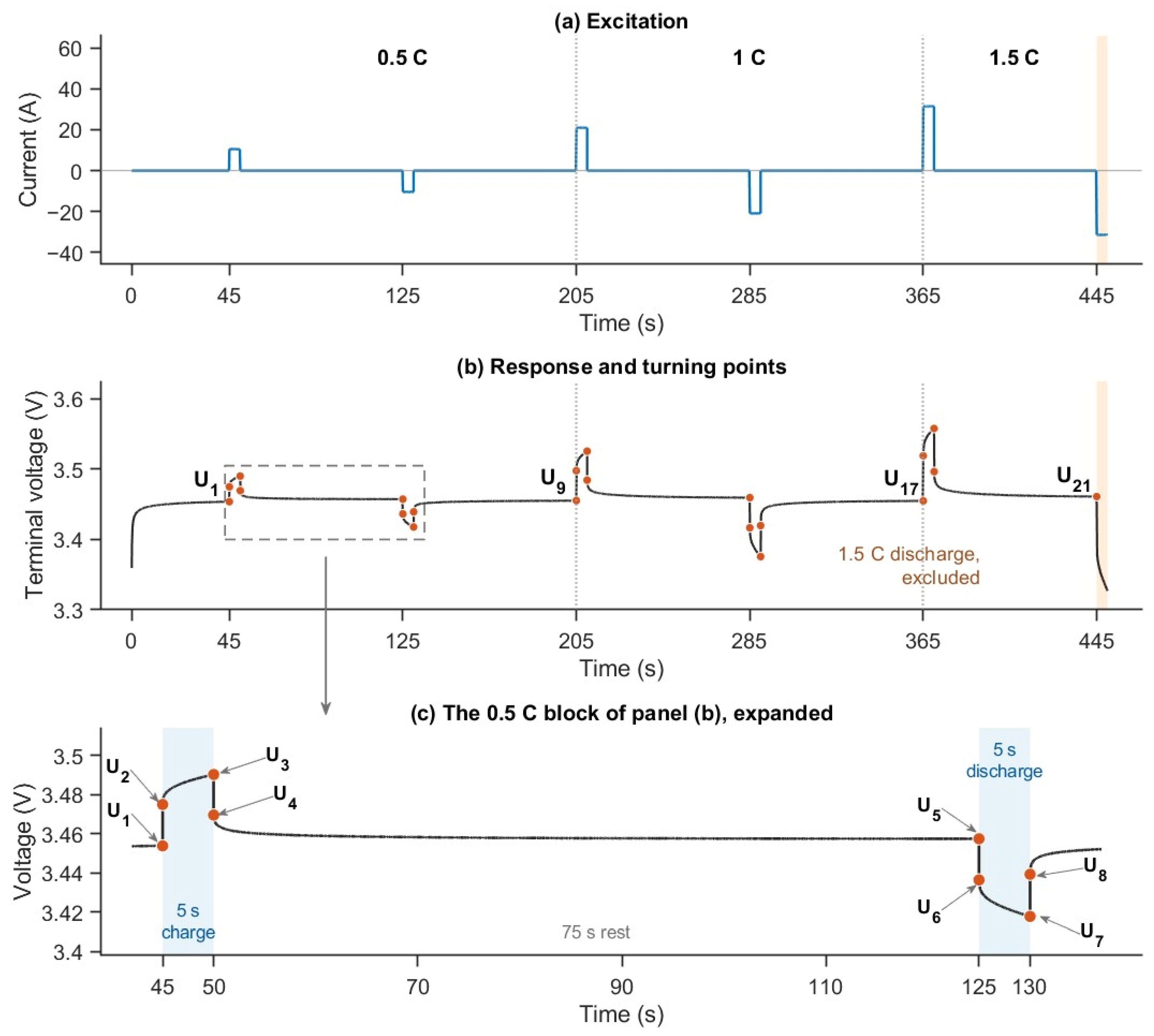
The identifiers are reproduced exactly as they appear in the analysis pipeline so that a reimplementation can be checked by name. Each identifier consists of a prefix, a mechanism, and a direction or amplitude, separated by underscores. The prefix RAW_ denotes a quantity taken directly from the published record, whilst ENG_ denotes a quantity computed from that record.
The mechanism token R denotes the ohmic step, RC the matched-C-rate form of that step, Pol polarisation growth, Relax the relaxation recovery fraction, Asym the charge-against-discharge asymmetry, NonLin the amplitude non-linearity ratio, and VdropNorm the volt_drop_norm analogue. Direction is denoted by chg for charge and dch for discharge. Amplitude is denoted by 0p5, 1p0, or 1p5 for the 0.5 C, 1 C, and 1.5 C blocks, respectively. The decimal point is represented by the letter p because a full stop is not used within an identifier.
The asymmetry identifiers include the quantity from which the asymmetry is formed, R or Pol, whereas directional descriptors include their direction. The non-linearity ratios include both amplitudes, represented as 10over05 and 15over10.
Identifiers are set upright and are neither italicised nor subscripted because they are names rather than mathematical quantity symbols. The entry n/a in the Equation column identifies the one feature read directly from the published record rather than derived using an equation.
Appendix B. Reimplementation Parameters
Appendix A provides the descriptor inventory, whilst this appendix collects the information required to rebuild the analysis from the published feature workbooks. Table A2 sets out the seven feature configurations, and Table A3 lists the numerical and procedural parameters. Nothing in either table introduces a new method or result. Each entry is defined previously in Section 2 or reported in Section 3, except the MATLAB implementation of the MRMR selection and of the Bayesian search, which is given only in Table A3. The purpose is to allow the analytical configuration to be reconstructed from the manuscript without requiring access to the original analysis pipeline.
Table A2.
The seven feature configurations; the number of features fitted in each is reported in Table 2. C2, C3, and C4 correspond to Cases 2, 3, and 4 of [18], whilst C0 and the three OCV-free counterpart configurations are introduced in the present study.
Table A3.
Parameters required to reimplement the analysis, with the subsection in which each is defined. Health thresholds are dimensionless fractions, whilst conditioning targets are percentages of the capacity basis stated in the corresponding row.
Appendix C. Supporting Results
This appendix contains the detailed results supporting Section 3.2, Section 3.4, Section 3.6 and Section 4.4. Each detailed result is referenced from the main text where the corresponding finding is reported.
Table A4 gives the health-shifted classification results by view, configuration, and learner. It contains the values from which the arm levels in Table 3 can be approximated and the per-chemistry recalls supporting the NMC analysis in Section 3.6. The corresponding per-battery-type results are provided in Table S3.
For each learner and configuration, macro-recall in Table A4 is the median across the seeded fits where replication applies. Table S3 additionally contains per-battery-type recalls from the single replicate attaining the median macro-recall. These values are not obtained by reducing each per-type column separately across fits and therefore need not reconcile with the per-class medians in Table A4.
The OCV-retaining and OCV-free arm levels in Table 3 can be approximated by taking means of the values shown in Table A4, with differences no greater than 0.002. The arm gaps and the percentage removed by matching are not formed by this route. Each is calculated within a replicate before the median is taken across the 25 replicate indices. Recalculating these quantities from the already reduced values in Table A4 can therefore change the final reported digit. The chemistry-resolved arm gaps reported in Section 3.4 and provided in Table S5 are formed in the same way from the recall of each chemistry, and are likewise not obtained from the reduced values in Table A4.
The two-class sensitivity analysis reported in Section 4.4 is derived from the per-class recall columns of Table A4. Figure A2 supports the search-budget statement in Section 3.2.
Table A4.
Health-shifted classification by view, configuration, and learner, over 101 training rows at or above 0.88 SoH and 108 test rows below 0.85 SoH. The replicate range is the range of macro-recall over the seeded fits, not a confidence interval, and is zero by construction for deterministic learners. For bagged-tree rows, each metric column is reduced separately by its median across the 25 seeded fits, so the per-class recall medians need not average exactly to the macro-recall shown.
Figure A2.
Automated-search convergence for the seven feature configurations, showing the best observed objective, dimensionless, against the evaluation index over the declared budget of 100 evaluations. One line represents each configuration. The flat tail of each curve shows the range of evaluations over which the budget produced no further improvement. The inset enlarges the objective range from 0 to 0.05.
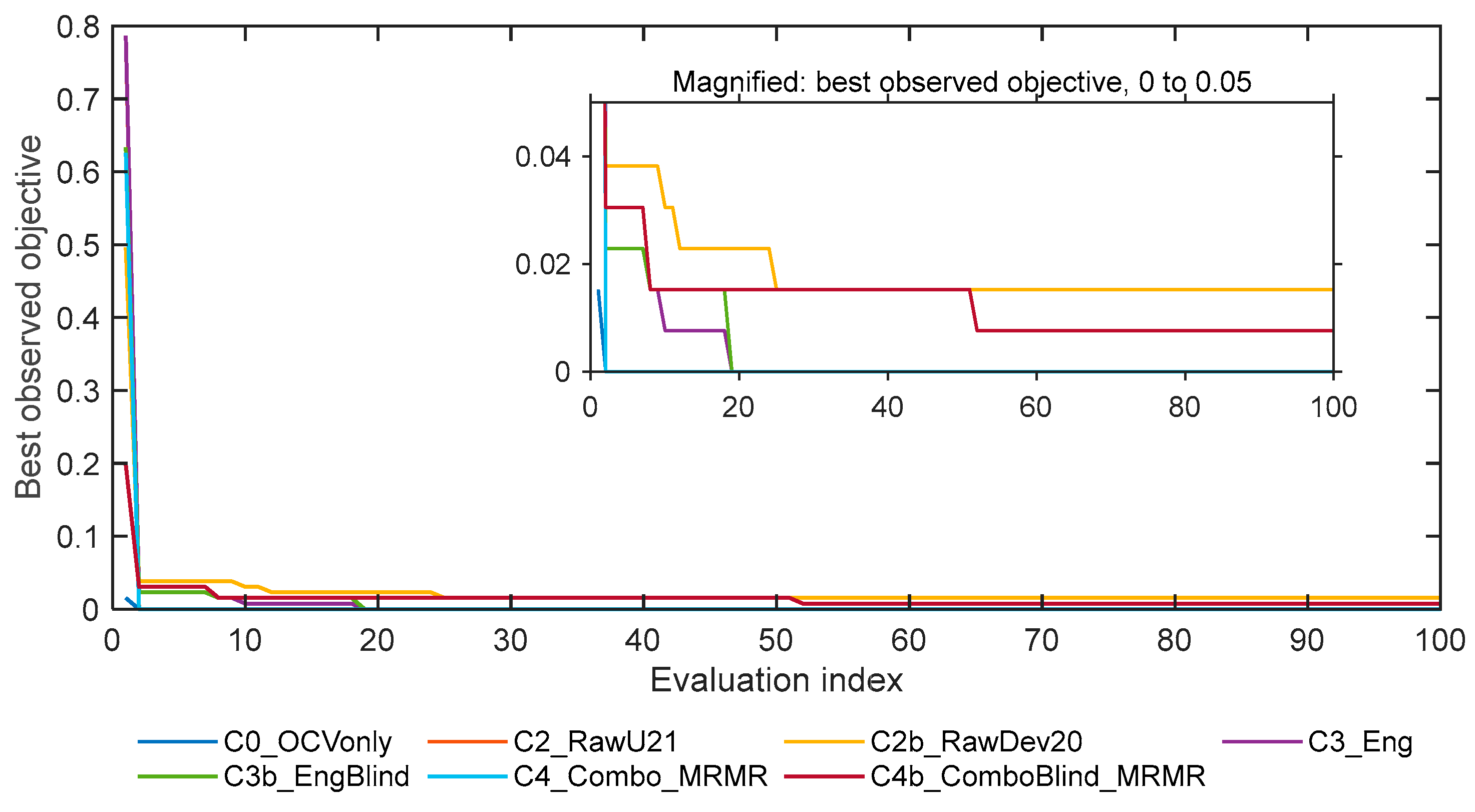
The two-class arm difference reported in Section 4.4, +0.09 in View A and −0.06 in View B, is calculated from the per-class recalls in Table A4. Removing NMC changes the task from three classes to two and raises the chance level for macro-recall from 0.333 to 0.500. The two-class and three-class quantities are therefore not directly comparable.
The sign reversal between the views is associated with C0_OCVonly under LDA, where LFP recall falls to 0.033 in View B. When that learner-configuration combination is excluded, the View B difference is −0.006. When the complete C0_OCVonly configuration is excluded, the View B difference is +0.008. The same combination of configuration and learner also mainly drives the negative LFP gap in View B in the chemistry-resolved analysis of Section 3.4.
The +0.09 and −0.06 differences are average per-class recall values that have already been reduced across fits rather than forming a two-class quantity within each replicate. They should therefore be regarded as indicative sensitivity quantities rather than as results constructed on the same basis as the arm gap in Table 3. The reduced test population contains 30 LFP rows and 36 LMO rows, giving 66 rows from 66 physical cells. Unlike the complete 108-row test set, it contains no repeated battery-states from the same physical cell.
References
- Harper, G.; Sommerville, R.; Kendrick, E.; Driscoll, L.; Slater, P.; Stolkin, R.; Walton, A.; Christensen, P.; Heidrich, O.; Lambert, S.; et al. Recycling lithium-ion batteries from electric vehicles. Nature 2019, 575, 75–86. [Google Scholar] [CrossRef] [Scilit] [PubMed]
- International Energy Agency. Global EV Outlook 2024; International Energy Agency: Paris, France, 2024; Available online: https://www.iea.org/reports/global-ev-outlook-2024 (accessed on 5 April 2026).
- Morse, I. A dead battery dilemma. Science 2021, 372, 780–783. [Google Scholar] [CrossRef] [Scilit] [PubMed]
- Tao, S.; Moura, S.; Brandell, D.; Han, Z.; Urréhman, S.; Zou, C.; Zhang, X.; Zhou, G. Artificial intelligence for battery reuse, recycling and remanufacturing. Nat. Rev. Clean. Technol. 2026, 2, 366–381. [Google Scholar] [CrossRef] [Scilit]
- Chen, Q.; Hou, Y.; Lai, X.; Shen, K.; Gu, H.; Wang, Y.; Guo, Y.; Lu, L.; Han, X.; Zheng, Y. Evaluating environmental impacts of different hydrometallurgical recycling technologies of the retired nickel-manganese-cobalt batteries from electric vehicles in China. Sep. Purif. Technol. 2023, 311, 123277. [Google Scholar] [CrossRef] [Scilit]
- Neumann, J.; Petranikova, M.; Meeus, M.; Gamarra, J.D.; Younesi, R.; Winter, M.; Nowak, S. Recycling of lithium-ion batteries—Current state of the art, circular economy, and next generation recycling. Adv. Energy Mater. 2022, 12, 2102917. [Google Scholar] [CrossRef] [Scilit]
- Olivetti, E.A.; Ceder, G.; Gaustad, G.G.; Fu, X. Lithium-ion battery supply chain considerations: Analysis of potential bottlenecks in critical metals. Joule 2017, 1, 229–243. [Google Scholar] [CrossRef] [Scilit]
- Wu, Z.; Zhao, Z.; Fang, Z.; Bao, H.; Liu, P.; Su, X.; Zhang, Y.; Jin, K.; Li, H.; Wang, Q. Rapid sorting of retired lithium-ion batteries using novel sorting feature extraction and a two-step classification method. J. Power Sources 2025, 654, 237845. [Google Scholar] [CrossRef] [Scilit]
- Liu, X.; Tang, Q.; Feng, Y.; Lin, M.; Meng, J.; Wu, J. Fast sorting method of retired batteries based on multi-feature extraction from partial charging segment. Appl. Energy 2023, 351, 121930. [Google Scholar] [CrossRef] [Scilit]
- Liu, T.; Chen, X.; Peng, Q.; Peng, J.; Meng, J. An enhanced sorting method for retired battery with feature selection and multiple clustering. J. Energy Storage 2024, 87, 111422. [Google Scholar] [CrossRef] [Scilit]
- Wang, Y.-C.; Chen, K.-C. Classification of aged batteries based on capacity and/or resistance through machine learning models with aging features as input: A comparative study. J. Clean. Prod. 2024, 471, 143431. [Google Scholar] [CrossRef] [Scilit]
- Tao, S.; Liu, H.; Sun, C.; Ji, H.; Ji, G.; Han, Z.; Gao, R.; Ma, J.; Ma, R.; Chen, Y.; et al. Collaborative and privacy-preserving retired battery sorting for profitable direct recycling via federated machine learning. Nat. Commun. 2023, 14, 8032. [Google Scholar] [CrossRef] [Scilit] [PubMed]
- Parambu, R.B.K.; Farrag, M.E.; Gowaid, I.A.; Ibem, C.N. AutoML-assisted classification of Li-ion cell chemistries from cycle life data: A scalable framework for second-life sorting. Energies 2025, 18, 5738. [Google Scholar] [CrossRef] [Scilit]
- Tao, S.; Ma, R.; Zhao, Z.; Ma, G.; Su, L.; Chang, H.; Chen, Y.; Liu, H.; Liang, Z.; Cao, T.; et al. Generative learning assisted state-of-health estimation for sustainable battery recycling with random retirement conditions. Nat. Commun. 2024, 15, 10154. [Google Scholar] [CrossRef] [Scilit] [PubMed]
- Tao, S.; Ma, R.; Chen, Y.; Liang, Z.; Ji, H.; Han, Z.; Wei, G.; Zhang, X.; Zhou, G. Rapid and sustainable battery health diagnosis for recycling pretreatment using fast pulse test and random forest machine learning. J. Power Sources 2024, 597, 234156. [Google Scholar] [CrossRef] [Scilit]
- Tao, S.; Guo, R.; Lee, J.; Moura, S.; Canals Casals, L.; Jiang, S.; Shi, J.; Harris, S.; Zhang, T.; Chung, C.Y.; et al. Immediate remaining capacity estimation of heterogeneous second-life lithium-ion batteries via deep generative transfer learning. Energy Environ. Sci. 2025, 18, 7413–7426. [Google Scholar] [CrossRef] [Scilit]
- Hu, H.; Huang, X.; Liang, C.; Lyu, Z.; Su, L.; Li, K.; Qin, Z.; Mo, H.; Zhang, X.; Zou, C.; et al. Second-level heterogeneous retired battery type identification using pulse-test-enabled federated learning with output-level privacy preservation. eTransportation 2026, 29, 100607. [Google Scholar] [CrossRef] [Scilit]
- Parambu, R.B.K.; Farrag, M.E.; Gowaid, I.A. AutoML-based framework for battery cell chemistry classification using short measurements: Towards efficient recycling. World Electr. Veh. J. 2026, 17, 391. [Google Scholar] [CrossRef] [Scilit]
- Tao, S.; Ma, G.; Yang, H.; Lu, M.; Wei, G.; Zhou, G.; Zhang, X. PulseBat: A field-accessible dataset for second-life battery diagnostics from realistic histories using multidimensional rapid pulse test. arXiv 2025, arXiv:2502.16848. [Google Scholar] [CrossRef] [Scilit]
- Barai, A.; Uddin, K.; Widanage, W.D.; McGordon, A.; Jennings, P. A study of the influence of measurement timescale on internal resistance characterisation methodologies for lithium-ion cells. Sci. Rep. 2018, 8, 21. [Google Scholar] [CrossRef] [Scilit] [PubMed]
- Ding, C.; Peng, H. Minimum redundancy feature selection from microarray gene expression data. J. Bioinform. Comput. Biol. 2005, 3, 185–205. [Google Scholar] [CrossRef] [Scilit] [PubMed]
- Breiman, L. Bagging predictors. Mach. Learn. 1996, 24, 123–140. [Google Scholar] [CrossRef] [Scilit]
- Nitta, N.; Wu, F.; Lee, J.T.; Yushin, G. Li-ion battery materials: Present and future. Mater. Today 2015, 18, 252–264. [Google Scholar] [CrossRef] [Scilit]
- Edge, J.S.; O’Kane, S.; Prosser, R.; Kirkaldy, N.D.; Patel, A.N.; Hales, A.; Ghosh, A.; Ai, W.; Chen, J.; Yang, J.; et al. Lithium ion battery degradation: What you need to know. Phys. Chem. Chem. Phys. 2021, 23, 8200–8221. [Google Scholar] [CrossRef] [Scilit] [PubMed]
- Yang, Z.; Hwang, T.; Mu, Y.; Luo, J.; Perruci, G.F.; Lu, H.; Cho, K.; Zhou, Y. Understanding the mechanistic role of reversible Li–Ag alloy interphases in ultralong-cycle lithium-metal batteries. Chem. Eng. J. 2025, 524, 169212. [Google Scholar] [CrossRef] [Scilit]
- Regulation (EU) 2023/1542 of the European Parliament and of the Council of 12 July 2023 concerning batteries and waste batteries, amending Directive 2008/98/EC and Regulation (EU) 2019/1020 and repealing Directive 2006/66/EC. Off. J. Eur. Union 2023, L 191, 1–117. Available online: https://eur-lex.europa.eu/eli/reg/2023/1542/oj (accessed on 15 October 2026).
- Huang, X.; Tao, S.; Liang, C.; Tang, Y.; Chen, J.; Shi, J.; Li, Y.; Xia, B.; Zhou, G.; Zhang, X. iMOE: Prediction of second-life battery degradation trajectory using interpretable mixture of experts. Nat. Commun. 2026, 17, 2549. [Google Scholar] [CrossRef] [Scilit] [PubMed]
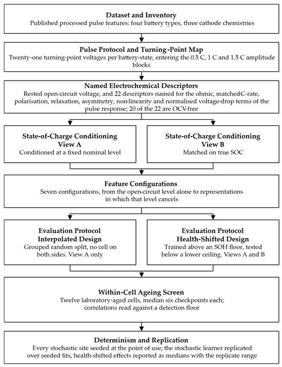
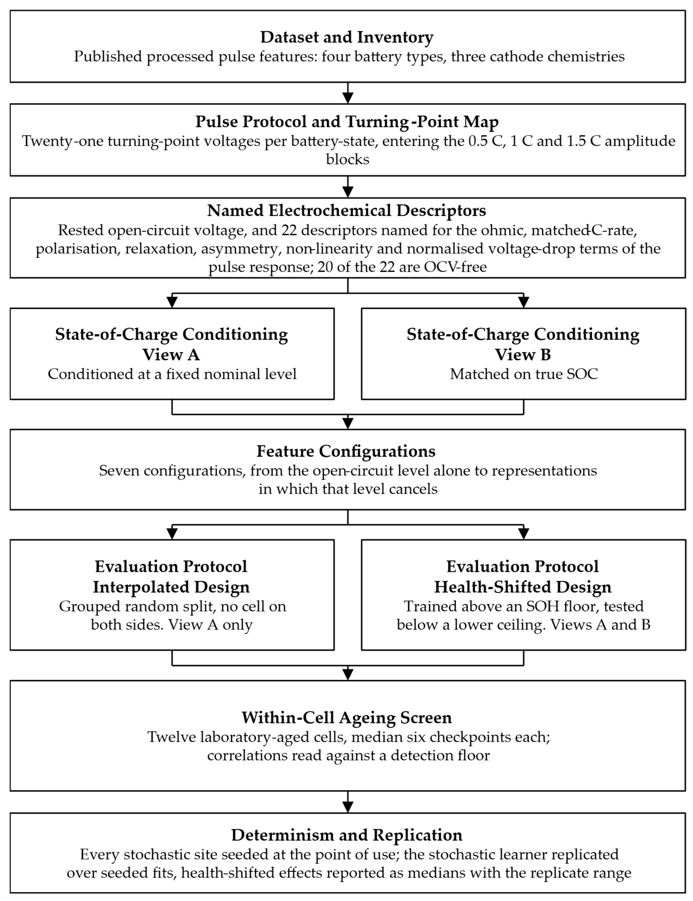
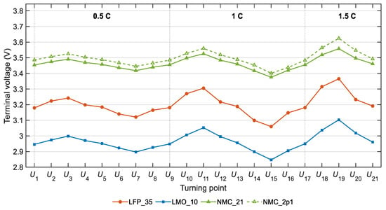
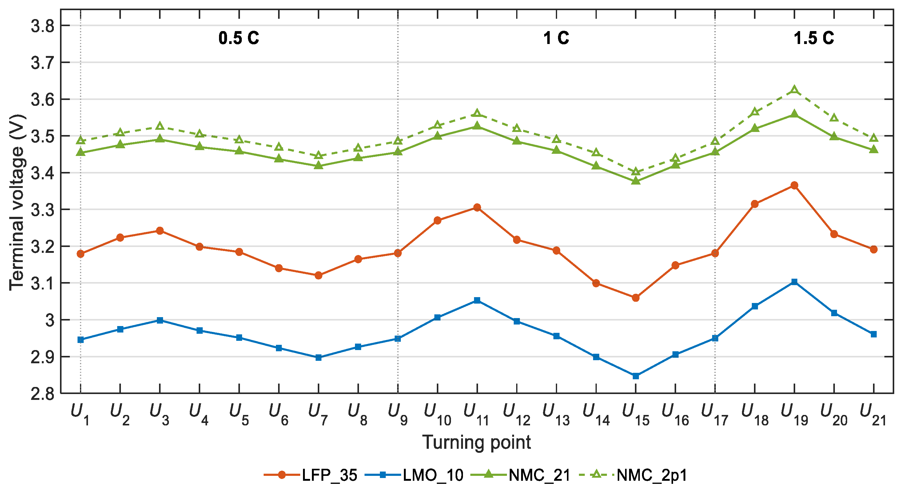
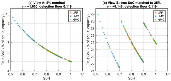
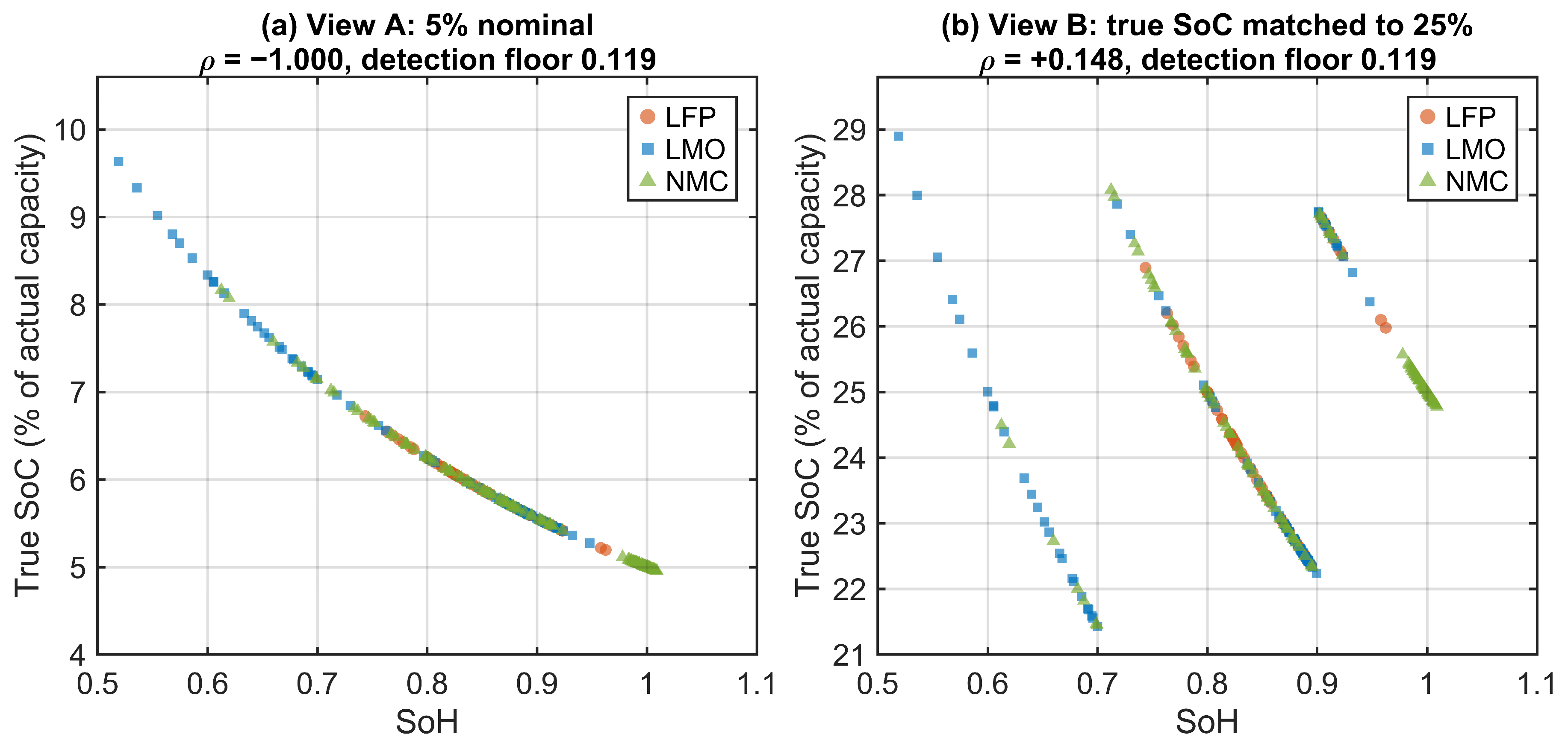
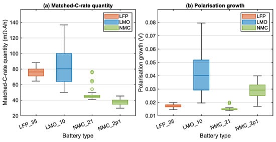
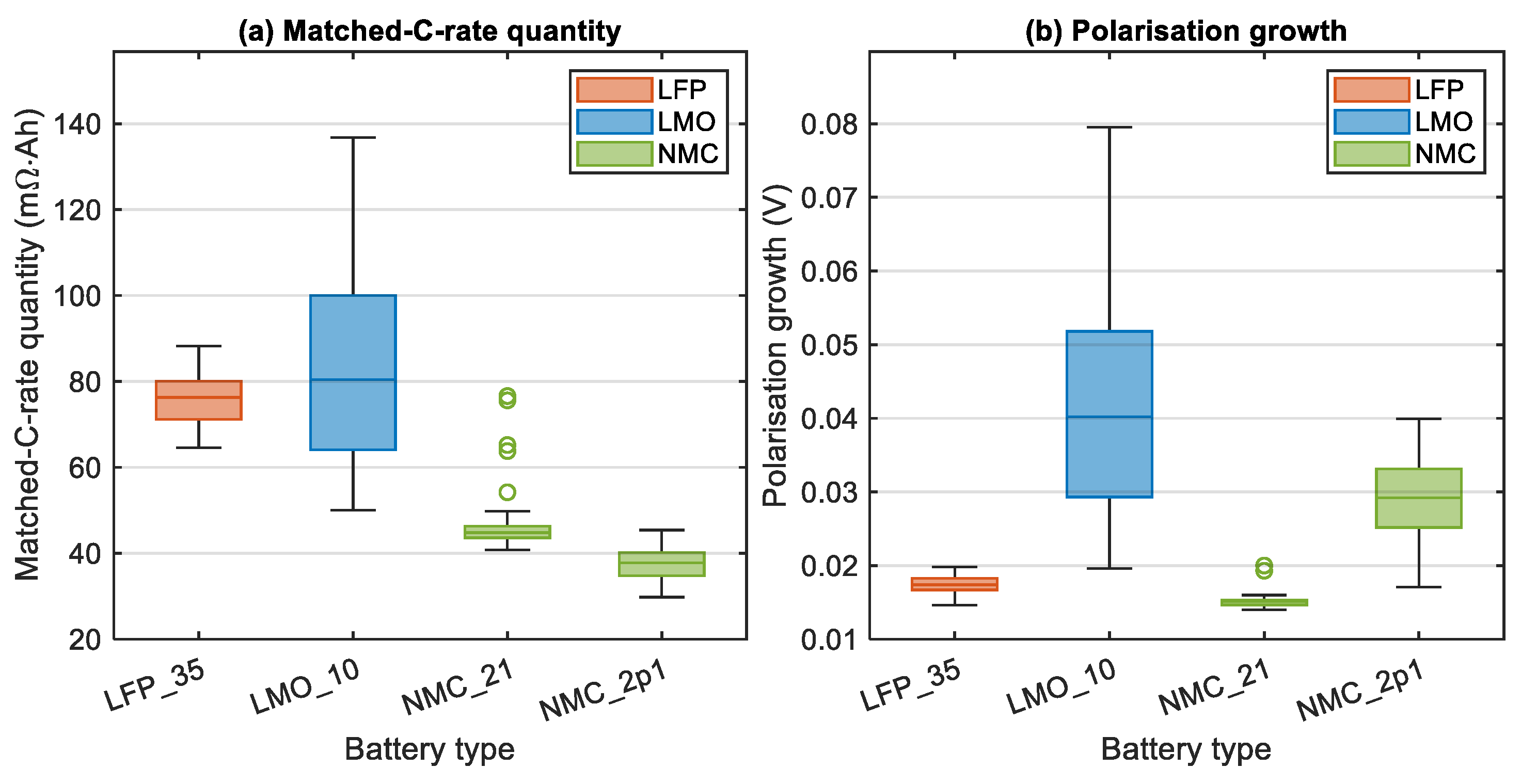
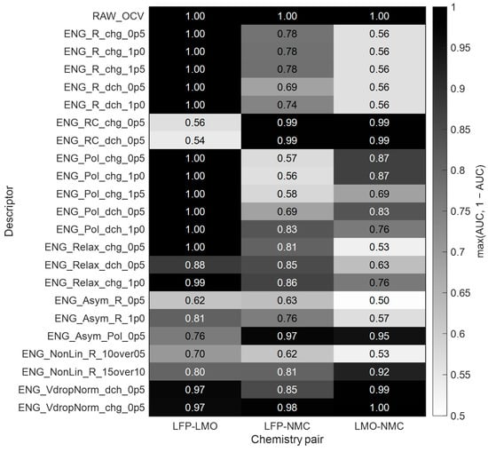
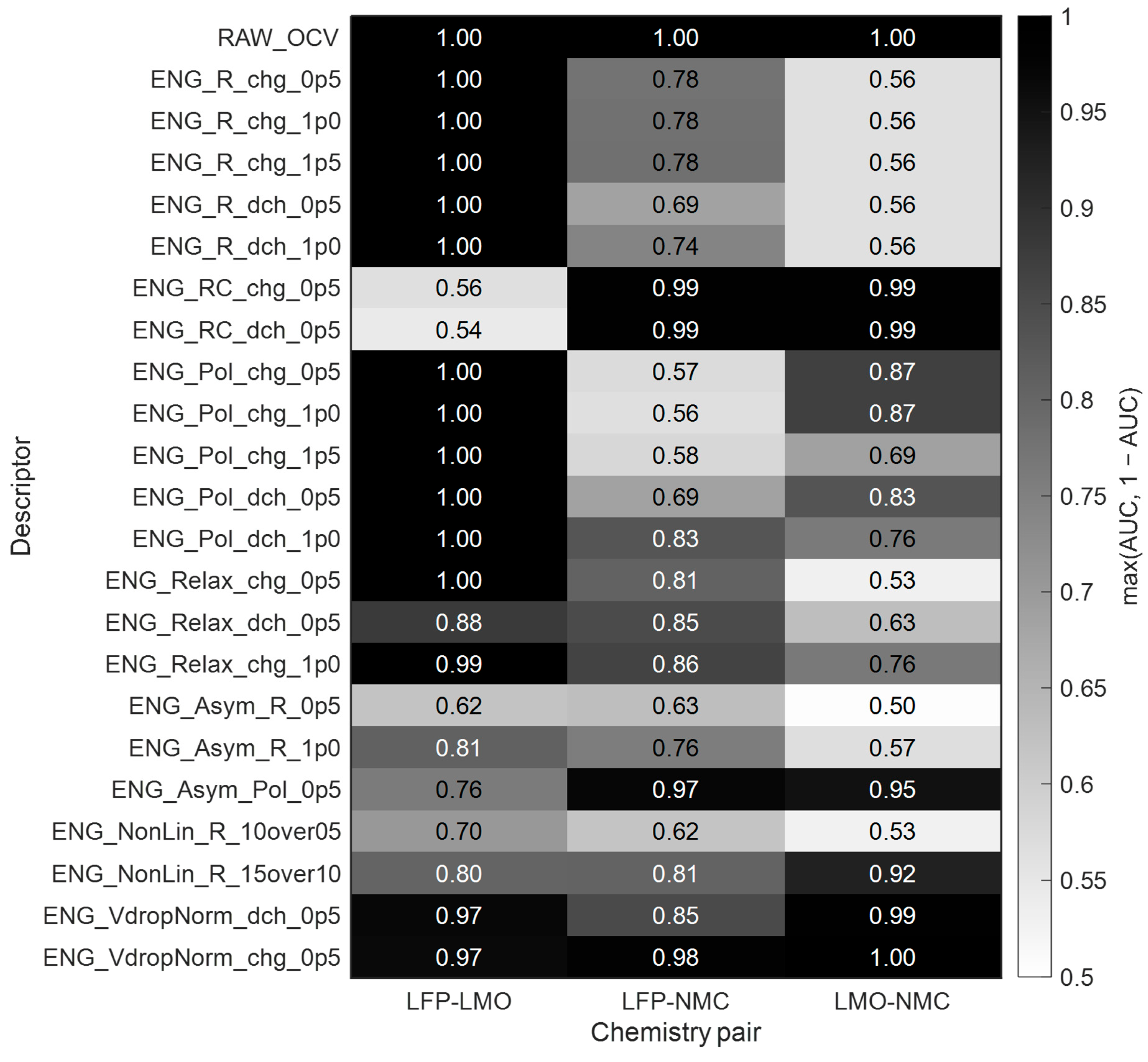
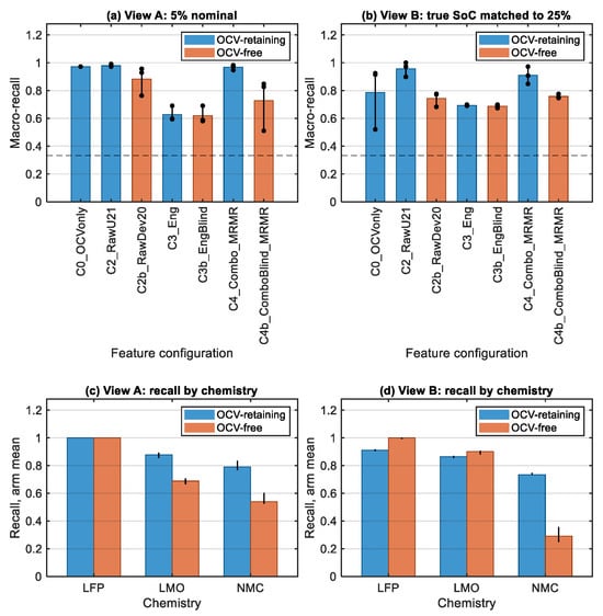
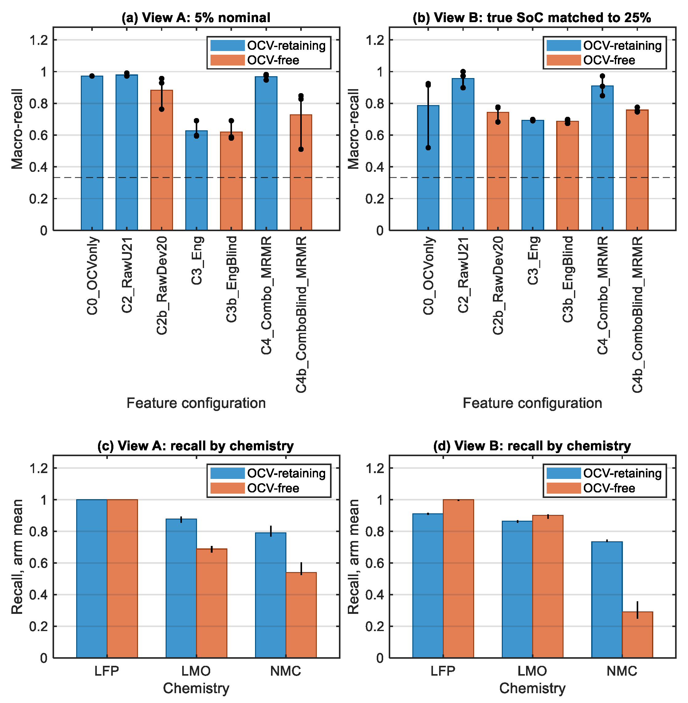
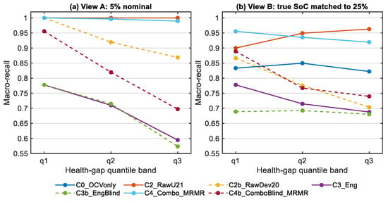
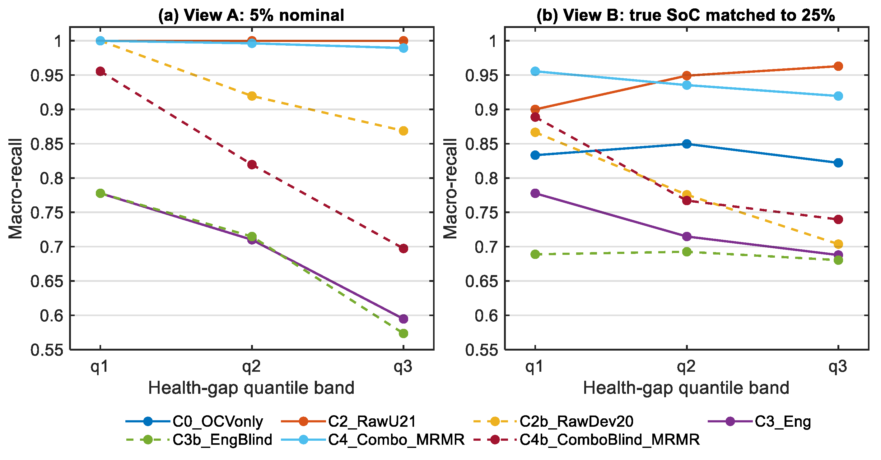
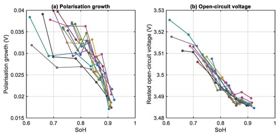
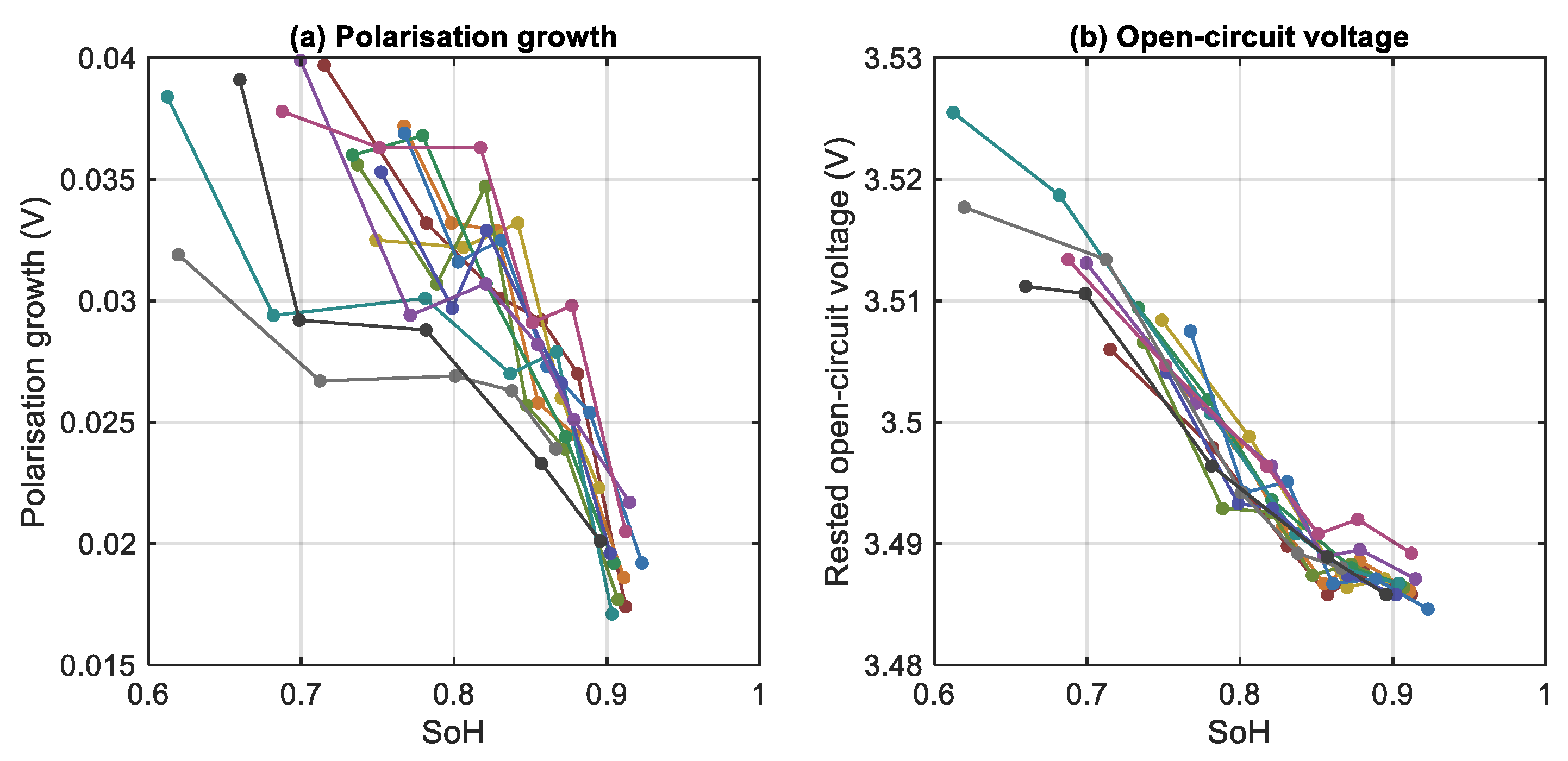

Disclaimer/Publisher’s Note: The statements, opinions and data contained in all publications are solely those of the individual author(s) and contributor(s) and not of MDPI and/or the editor(s). MDPI and/or the editor(s) disclaim responsibility for any injury to people or property resulting from any ideas, methods, instructions or products referred to in the content. |
© 2026 by the authors. Licensee MDPI, Basel, Switzerland. This article is an open access article distributed under the terms and conditions of the Creative Commons Attribution (CC BY) license.