


Abstract
Battery energy storage systems (BESSs) play a vital role in contemporary smart grids, but their increasing digitalisation exposes them to sophisticated cyberattacks. Existing anomaly detection approaches typically treat sensor measurements as flat feature vectors, overlooking the intrinsic relational structure of cyber–physical systems. This work introduces an enhanced Graph Neural Network (GNN) autoencoder for unsupervised BESS anomaly detection that integrates multiscale graph construction, multi-head graph attention, manifold regularisation via latent compactness and graph smoothness, contrastive embedding shaping, and an ensemble anomaly scoring mechanism. A comprehensive evaluation across seven BESS and firmware cyberattack datasets demonstrates that the proposed method achieves near-perfect Receiver Operating Characteristic (ROC) and Precision–Recall Area Under the Curve (PR AUC) (up to 1.00 on several datasets), outperforming classical one-class models such as Isolation Forest, One-Class Support Vector Machine (One-Class SVM), and Local Outlier Factor on the most challenging scenarios. These results illustrate the strong potential of graph-informed representation learning for cybersecurity monitoring in distributed energy resource infrastructures.
1. Introduction
Battery energy storage systems (BESSs) are becoming indispensable assets in modern electric grids due to their ability to support renewable integration, improve voltage stability, mitigate congestion, and enhance overall system resilience. Their increasing adoption coincides with a rapid trend toward digitalisation: supervisory control, remote inverter configuration, firmware updates, and cloud-based monitoring are now standard components of BESS operation. While these capabilities yield operational benefits, they also introduce significant cybersecurity risks. Malicious manipulation of measurements or control signals can induce oscillatory behaviour, trigger overlimit conditions, conceal battery degradation, or in extreme cases compromise the physical safety and reliability of the installation.
A large body of prior work has demonstrated the usefulness of anomaly detection algorithms for cyber–physical security in power systems. Classical approaches include statistical residual analysis, physics-informed consistency checks, and machine learning techniques such as Isolation Forest and One-Class SVM. Deep learning models—particularly autoencoders—have shown strong promise by learning compact representations of nominal behaviour and detecting deviations as reconstruction errors. However, these models typically process sensor data as independent multivariate vectors, failing to account for the relational structure among system components. In cyber–physical systems such as BESSs, where electrical, thermal, and communication couplings underpin system dynamics, ignoring structural dependencies limits detection sensitivity and interpretability.
Graph Neural Networks (GNNs) are explicitly designed for learning representations over relational domains [1]. They integrate information from neighbouring nodes through message passing, enabling the extraction of structural patterns in addition to local features. When applied to cyber–physical infrastructures, GNNs can capture the topological and functional dependencies between sensors, cells, and controllers, providing a more expressive model of the BESS behaviour. Recent work in power system cybersecurity has shown that graph-based models can enhance the detection of stealthy attacks, but existing graph autoencoders often employ a single-scale neighbourhood, fixed convolutional aggregation, or reconstruction-only anomaly scoring, which may be insufficient in heterogeneous or high-variability operating regimes.
This work introduces an Enhanced Graph Neural Network Autoencoder for unsupervised anomaly detection in BESS environments. The proposed method incorporates multiple architectural and algorithmic innovations to address limitations of previous approaches:
- Multiscale graph construction: Three weighted k-nearest neighbour graphs (with ) are combined to capture both local and mid-range structural relationships among samples.
- Multi-head graph attention encoder: A stack of attention layers with residual connections learns informative latent embeddings by dynamically weighting neighbours based on their contextual relevance.
- Manifold regularisation: The latent space is shaped through compactness constraints, graph smoothness penalties, and a contrastive objective to enhance separability between nominal and anomalous patterns.
- Ensemble anomaly scoring: Six complementary metrics—reconstruction errors, latent neighbourhood distances, Mahalanobis deviation, and latent Isolation Forest score—are normalised and aggregated into a robust anomaly score.
We evaluate the Enhanced GNN on seven real-world BESS and firmware cyberattack datasets. The experiments demonstrate that the proposed method consistently achieves state-of-the-art performance, with ROC and PR AUC values close to 1.00 on several datasets, and exhibits superior stability compared to classical baselines. In the most challenging scenarios, the Enhanced GNN outperforms Isolation Forest, One-Class SVM, and Local Outlier Factor, demonstrating its ability to detect subtle cyber–physical deviations that lie off-manifold yet remain indistinguishable for non-graph-based detectors.
The remainder of this paper is structured as follows. Section 2 reviews related work in distributed energy resource (DER) cybersecurity and graph-based anomaly detection. Section 3 presents the proposed Enhanced GNN architecture. Section 4 describes the datasets, baselines, and evaluation pipeline. Section 5 reports and analyses the quantitative results. Section 6 provides a broader interpretation of the findings, and Section 7 concludes the paper.
2. Related Work
This section reviews prior work in two main areas: cybersecurity of distributed energy resources, with a focus on BESSs, and the use of Graph Neural Networks for anomaly detection in time-series and power system applications.
2.1. Cybersecurity in Distributed Energy Resources
Intrusion detection in power systems has been extensively studied across multiple grid components, including advanced metering infrastructures, digital substations, synchrophasors, SCADA systems, and related communication networks [2]. Machine-learning-based approaches for detecting cyberattacks in smart grids have been explored from different perspectives, including deep learning for stealthy attacks and insider threats [3]. In SCADA environments, anomaly detection (AD) methods are commonly classified into network- and content-based techniques, which analyse traffic and protocol fields, and physics-aware approaches that leverage measurements reflecting the underlying physical process [4]. A recent framework categorises commercial cybersecurity tools into network monitoring, endpoint protection, physics-based diagnostics, and integrated response systems [5]. While network-centric IDS are widely deployed, they may fail to detect attacks that alter system behaviour without significantly affecting traffic patterns [6]. This limitation is particularly critical in distributed energy resource (DER) settings, where effective detection requires joint monitoring of cyber and physical domains [7]. Physics-based monitoring therefore complements network analysis by assuming that successful attacks ultimately manifest as deviations in physical variables such as voltage, current, or frequency, often enabling earlier detection [8]. Surveys in [9,10] provide comprehensive overviews of physics-informed anomaly detection techniques. A key challenge for supervised learning in this context is the scarcity and imbalance of labelled attack data. As a result, novelty detection and one-class classification methods are frequently adopted to model normal system behaviour and identify deviations [11]. Among deep-learning approaches, autoencoder-based architectures are particularly popular for anomaly detection due to their representation-learning capabilities [12,13]. These models compress input data through an encoder and reconstruct it via a decoder, with anomalies detected from reconstruction errors.
Temporal extensions of autoencoders incorporate sequential dependencies using recurrent architectures such as RNNs, LSTMs, or GRUs [14,15]. For example, Harrou et al. integrate GRUs into autoencoders for power grid monitoring, while noting the limitations of relying on simulated attacks [16]. LSTM-based autoencoders have also been applied to wind turbine monitoring [17] and battery systems using variational autoencoders [18], though without explicit integration of physical knowledge. Cyber–physical integration is considered in [19], but physical system equations are not directly embedded in the learning process.
Physics-informed approaches aim to address this gap by incorporating domain knowledge into model training. Chen et al. guide LSTM training using physics-based constraints rather than explicitly embedding system equations [20]. More generally, physics-informed neural networks (PINNs) demonstrate strong generalisation capabilities even with limited datasets, making them well-suited for industrial cybersecurity applications [21]. This paradigm underpins the approach adopted in this work. The increasing penetration of DERs has brought cybersecurity concerns to the forefront of power system research and practice. Chen et al. [22] provide a comprehensive survey of cybersecurity for DER systems in the smart grid, covering vulnerabilities, attack vectors, and defence mechanisms across different layers of the architecture. The authors emphasise the need for -in-depth defence and for approaches that combine IT security mechanisms with cyber–physical modelling. False Data Injection Attacks (FDIAs) have been identified as a particularly serious threat to smart grids. By maliciously modifying sensor measurements, attackers can corrupt state estimation and mislead control decisions while remaining undetected by traditional bad data detection [23]. Boyaci et al. [24] proposed one of the first GNN-based frameworks for the joint detection and localisation of stealth FDIAs in power systems, demonstrating that graph-based methods can effectively exploit the spatial correlations inherent in network topology. For BESSs specifically, research has explored both data-driven and physics-based detection strategies. Kharlamova et al. [25] review data-driven approaches for the cyber defence of BESSs, including shallow- and deep-learning methods, and highlight the promise of neural network-based anomaly detection. Gaggero et al. [26] proposed an autoencoder-based algorithm that learns the normal behaviour of a BESS and detects anomalies that violate physical constraints, effectively combining data-driven and physics-based ideas. Their subsequent publication of the BESS-Set dataset [27] has provided a standardised benchmark for BESS cybersecurity, enabling systematic comparison of detection techniques.
Despite this progress, most existing BESS anomaly detection methods treat the system as a collection of independent or loosely coupled sensor time series. They generally do not leverage the explicit system topology (electrical, thermal, and communication), which limits their ability to model correlated effects and to localise attacks within the infrastructure.
2.2. Graph Neural Networks for Anomaly Detection
Graph Neural Networks have emerged as powerful tools for learning from graph-structured data, with successful applications in recommendation systems, social networks, chemistry, and, more recently, smart grids. The graph attention network (GAT) introduced by Veličković et al. [28] applies attention mechanisms to neighbourhood aggregation, enabling models to learn the relative importance of neighbours, rather than relying on fixed aggregation weights.
In the context of multivariate time-series anomaly detection, Zhao et al. [29] proposed a GNN-based framework that leverages graph attention to model dependencies between different variables. Their work demonstrated that GNNs can capture both spatial and temporal patterns, outperforming traditional sequence models such as LSTMs on several benchmarks. Combining reconstruction- and forecasting-based objectives has also been shown to improve the robustness of learned representations for anomaly detection in time series.
In power system cybersecurity, GNNs have been employed primarily for FDIA detection and localisation in transmission and distribution networks [24]. These methods typically treat buses, substations, or meters as graph nodes and use power network topology as the underlying graph. However, the explicit application of GNNs to BESS cybersecurity is still limited. Existing BESS-focused methods rely largely on autoencoders or classical machine learning approaches that overlook the graph structure of cells, sensors, and controllers [25,26].
The present work aims to bridge this gap by defining a graph representation tailored to BESSs and developing a spatio-temporal GNN architecture that captures both the topological and the dynamic behaviour of the system. By leveraging graph attention mechanisms and a dual-branch autoencoder design, the proposed model can provide both high detection performance and interpretable anomaly localisation.
3. Methodology
This section presents the proposed Enhanced Graph Neural Network Autoencoder (Enhanced GNN-AE) designed for unsupervised anomaly detection in battery energy storage systems. The architecture integrates multiscale graph construction, a multi-head graph attention encoder, manifold regularisation through latent compactness and graph smoothness, contrastive embedding shaping, and a robust ensemble anomaly scoring mechanism.
The full processing pipeline is illustrated in Figure 1.
Figure 1.
Overview of the proposed Enhanced GNN Autoencoder anomaly detection pipeline, comprising multiscale graph construction, multi-head graph attention encoding, manifold-regularised latent representations, and ensemble anomaly scoring.
The implementation can follow different strategies; the algorithm could run directly on the control node, such as the inverter, but this may be difficult due to hardware constraints. Alternatively the information extraction process can be done by sniffing traffic on an intermediate node. The network sniffer could be a script specifically designed to decode fieldbus protocol, such as Modbus TCP frames. It operates on the application layer to passively monitor traffic between a client and server. The process follows these steps:
- Passive Capture: Data is collected at an intermediate node, such as a network switch, to ensure no interference with the primary communication flow.
- Payload Decoding: The sniffer extracts the payload from the intercepted packets.
- Feature Mapping: It reconstructs the values for 22 distinct physical features, such as irradiance, phase currents, and power setpoints.
Regardless of the implementation, the structure of the algorithm remains the same, and is detailed below.
Possible False Positives may arise when the model has to handle concept drift, such as gradual battery degradation or seasonal changes. The expected behaviour of an anomaly detection algorithm is to generalise the limits of the training dataset. While the dataset includes fluctuations in energy demand and varying environmental conditions, the primary goal is for the algorithm to recognise significant variations from the established “normal” behaviour captured during the training phase; for these reasons, a simple training should be enough to handle these situations. On the contrary, it would be possible to repeat the training phase, adding new data in different seasonal working conditions.
3.1. Multiscale Graph Construction
Given a training dataset of normal-operation samples
we construct three k-nearest neighbour (kNN) graphs using . For each k, distances are computed using Euclidean metrics, and edges are assigned weights via a Gaussian kernel:
where denotes the median non-zero neighbour distance for neighbourhood size k.
Each adjacency matrix is symmetrised and normalised using
where is the degree matrix. The reasons why we symmetrise a directed kNN graph include
- Standard kNN produces directed edges: (i has j as neighbour), but necessarily.
- Symmetrising via creates undirected edges: if i and j are close in feature space, they should influence each other mutually.
- For anomaly detection: similarity should be symmetric—if sample A is anomalous relative to B, then B is similarly anomalous relative to A.
Spectral normalisation ensures the graph convolution operator has bounded spectral properties. It prevents gradient explosion during backpropagation and improves numerical stability and empirically symmetric normalisation improves training stability vs. asymmetric alternatives.
The final adjacency matrix aggregates the three scales:
providing a richer representation of both local and meso-scale relationships.
3.2. Topological Feature Augmentation
To enhance graph expressiveness, we derive additional geometric descriptors for each sample:
- Average neighbour distance: ;
- Maximum neighbour distance: ;
- Local density: ;
- Variance of distances: ;
- Nearest-neighbour distance: .
These five descriptors are concatenated to the raw feature vector
This augmentation enables the model to capture density irregularities and local geometric distortions that may signify cyber–physical anomalies.
3.3. Enhanced Graph Attention Encoder
The encoder is based on stacked graph attention (GAT) layers. Each layer computes
where
- M is the number of attention heads;
- is the projection matrix for head m;
- is the learned attention coefficient computed via
Two architectural refinements improve stability:
- Residual connections between consecutive GAT layers:which mitigate vanishing gradients and preserve coarse information.
- Batch normalisation and dropout, improving generalisation and reducing overfitting.
The output of the final GAT layer is a compact latent embedding .
3.4. Decoder and Reconstruction
A feed-forward decoder reconstructs the input from its latent embedding:
using two hidden layers with ELU activations and batch norm. The reconstruction objective alone, however, is insufficient for sharp anomaly boundaries; thus, several regularisation terms are introduced.
3.5. Manifold Regularisation
To shape the latent manifold and enhance separability between normal and anomalous points, three regularisers are applied.
3.5.1. Latent Compactness
Nominal samples should cluster around a central latent prototype:
where is the mean latent vector.
3.5.2. Graph Smoothness
The latent representation should respect multiscale graph structure:
penalising abrupt changes across the graph.
3.5.3. Contrastive Regularisation
A contrastive term encourages embeddings of normal samples to form a tight manifold:
where is cosine similarity and is a temperature parameter. Table 1 reports a sensitivity analysis of the contrastive loss with respect to the temperature parameter across different similarity measures. For all considered metrics, performance improves as increases from 0.1, reaching a maximum around , after which a gradual degradation is observed. The cosine similarity consistently achieves the highest scores, indicating a better alignment with the underlying representation space compared to Euclidean, Pearson, and dot-product similarities. Notably, the optimal temperature value is shared across all similarity functions, suggesting that the contrastive objective is relatively robust to the choice of similarity metric when is appropriately tuned. The temperature parameter controls the sharpness of the softmax function in contrastive learning. We empirically select via grid search, and find to be optimal for BESS anomaly detection.
Table 1.
Contrastive loss sensitivity analysis.
3.6. Overall Training Objective
The end-to-end loss combines reconstruction and regularisation:
3.7. Ensemble Anomaly Scoring
At inference time, six complementary metrics are computed:
Each metric is normalised to , and the final anomaly score is
where are tuned ensemble weights. A detection threshold is obtained via percentile sweep, maximising the macro F1 score.
4. Experimental Setup
This section describes the datasets used for evaluation, the preprocessing pipeline, the hyperparameter optimisation strategy, the baseline models, and the evaluation metrics adopted to benchmark the proposed Enhanced GNN Autoencoder.
4.1. Datasets
Experiments were conducted using the BESS-Set dataset, a publicly available resource designed for BESS cybersecurity research. A more detailed explanation of the dataset can be found in [27]. The dataset is generated from a detailed Simulink model of a grid-connected BESS and includes time-series measurements under both normal operating conditions and a variety of simulated cyberattack scenarios.
Data characteristics: BESS-Set contains measurements for key BESS variables, including cell- and pack-level voltage, current, temperature, and SoC (State of Charge). In our experiments, we used a subset of these features and derived additional ones such as the first-order derivatives of voltage, current, and temperature, resulting in an eight-dimensional feature vector per node and timestep.
The data consists of physical measurements, such as those exchanged between the BESS inverter and a Supervisory Control and Data Acquisition (SCADA) system, and were extracted from an electromagnetic simulation model implemented MATLAB/Simulink 9.13.0 (r2022b). System functioning is recorded at a 1-second sampling time
Attack scenarios: The dataset includes several cyberattack types relevant to BESS. The simulated cyberattacks are categorised into three main types targeting distributed energy resources (DERs):
- Bad Data Injection: Modifying commands, such as power setpoints, potentially causing the BESS to exceed operational limits or introduce oscillations.
- False Data Injection: Tampering with measurements reported back to the main controller (e.g., modifying the State of Charge (SoC) or active power measures) to induce wrong decisions.
- Firmware Modification: Altering the internal functioning of the inverter, which can lead to severe consequences such as the injection of harmonics into the grid or modification of battery voltage control.
The dataset is organised into 9 files, with features resulting in datasets containing either 13 or 14 columns. The dimensions and structure of the BESS-Set files are summarised below in Table 2. The training data file contains around 30,000 rows and 13 features representing normal operations. The anomaly files have 14 columns, where the final column serves as the label (0 for normal behaviour, 1 for anomaly).
Table 2.
Summary of .csv dataset files.
The BESS-Set is designed to accurately reflect the real-world physical behaviour of a BESS: the data is extracted from an electromagnetic simulation model (that is provided open source together with the data), and the attacks are not arbitrary, but they are based on a taxonomy of smart inverter threats. However, replicating the simulated cyberattacks in a real environment is strictly avoided due to the extreme risks they pose to physical infrastructure. Malicious manipulation of these systems can jeopardise the reliability of energy storage and threaten the stability of the broader power grid. Specific scenarios, such as firmware modifications that tamper with battery voltage control, are particularly dangerous as they can induce working conditions that cause permanent damage to the battery cells. Because attacks toward DERs can threaten the safety of the entire power system, these scenarios must be safely conducted within a controlled electromagnetic simulation environment to facilitate the development of monitoring algorithms without jeopardising critical assets.
4.2. Preprocessing and Feature Engineering
All continuous variables are standardised via Z-score normalisation:
using means and variances computed exclusively from the normal training pool.
To enrich the feature representation and improve sensitivity to cyber–physical deviations, we augment each sample with topological descriptors derived from its neighbourhood in feature space. These additional features include
- Mean neighbour distance;
- Maximum neighbour distance;
- Local density;
- Distance variance;
- Nearest neighbour distance.
These descriptors help the model discriminate between anomalies that are sparse, isolated, or geometrically inconsistent with the nominal manifold.
Data augmentation is applied to the normal dataset through low-level Gaussian perturbations:
which improves robustness and stabilises manifold learning.
4.3. Graph Construction
The multiscale graph described in Section 3 is constructed for both training and testing sets. For training, the adjacency matrix is computed once from the consolidated nominal dataset. For testing, a new graph is constructed for each dataset to reflect the true relational structure among unseen samples.
Since the proposed methodology treats each sample as a node in the graph, graph edges do not reflect spatial relations in the physical system but rather similarities in feature space; anomalies are expected to distort such relations.
4.4. Hyperparameter Optimisation
A comprehensive grid search explores architectural and regularisation (Table 3) of the Enhanced GNN-AE:
Table 3.
Hyperparameter search space.
- Hidden dimension ;
- Latent dimension ;
- Attention heads ;
- Neighbourhood scales or ;
- Latent compactness ;
- Graph smoothness ;
- Contrastive weight .
Each configuration is trained for 60 epochs with early stopping based on validation loss. To ensure robustness across heterogeneous datasets, model selection is guided by a composite score:
where is the average macro F1 across datasets and penalises poor worst-case behaviour.
The best configuration is retrained for 250 epochs to produce the final model.
4.5. Baseline Models
Three classical one-class anomaly detectors serve as baselines:
- Isolation Forest (IF) [11]: ensemble of random tree partitions.
- One-Class SVM (OC-SVM) [11]: kernel-based boundary estimation using RBF kernel.
- Local Outlier Factor (LOF) [11]: density-based anomaly measure comparing local neighbourhood density to that of its neighbours.
All baselines are trained exclusively on the standardised normal dataset. Their anomaly scores are negated so that larger values denote more abnormal behaviour. Thresholds are determined via macro F1 maximisation.
4.6. Evaluation Metrics
Detection performance were assessed using
- F1 score (macro);
- Accuracy;
- Balanced accuracy;
- Precision and recall;
- Matthews correlation coefficient (MCC);
- ROC AUC;
- PR AUC;
- Confusion matrices.
ROC and PR curves were generated to assess ranking performance independently of threshold. Confusion matrices (normalised and non-normalised) illustrate the distribution of detection errors.
4.7. Reproducibility
All experiments were conducted in Python (3.14) using PyTorch (2.9.1) on a workstation equipped with an NVIDIA GPU. Graphs were constructed using sparse tensor utilities, and hyperparameter search was fully automated. The enhanced metrics, grid-search scores, and per-dataset plots were exported to ensure full reproducibility.
5. Results
This section reports the quantitative performance of the proposed Enhanced GNN Autoencoder compared with three widely used one-class baselines: Isolation Forest, One-Class SVM, and Local Outlier Factor. Seven real-world anomaly detection datasets were considered, covering Bad Data Injection (BDI), false data injection (FDI), and firmware manipulation attacks.
Table 4 summarises the full set of results using the locally optimal decision threshold for each model and dataset. Performance is expressed in terms of macro F1, accuracy, ROC AUC, PR AUC, and Matthews correlation coefficient (MCC).
Table 4.
Performance comparison across all datasets for the Enhanced GNN and baseline anomaly detection models. Metrics are computed at the locally optimal threshold maximising macro . The Enhanced GNN achieves consistently strong performance and near-perfect detection on firmware manipulation datasets.
In Table 5 the averaged results across all datasets highlight clear differences in robustness and generalisation among the anomaly detection models. The Enhanced GNN demonstrates its ability to capture complex structural dependencies and subtle deviations from normal behaviour. Isolation Forest achieves competitive performance on some datasets, particularly those with well-separated anomaly clusters, but shows higher variability and lower discriminative ability in terms of ROC AUC. One-Class SVM exhibits moderate performance overall, struggling especially on datasets with non-linearly separable anomalies. Local Outlier Factor records the weakest results on average, confirming its limitations when applied to high-dimensional and heterogeneous feature spaces. Overall, the Enhanced GNN provides the most stable and accurate anomaly detection among the evaluated methods.
Table 5.
Average metrics on datasets for each anomaly detection method. Enhanced GNN shows overall superior performance, while Isolation Forest achieves excellent results on specific datasets but with higher variability.
Table 6 reports an ablation study analysing the individual and combined contributions of the anomaly detection metrics used in the proposed ensemble. Reconstruction-based metrics (L2 and L1) exhibit stable performance in terms of average F1 score and AUC, effectively capturing global deviations in the input space, although they show limited sensitivity to localised anomalies. Latent kNN-based metrics exhibit higher discriminative power, particularly when utilising the mean distance, underscoring the importance of preserving local manifold consistency for detecting density-based attacks. In contrast, the max kNN variant is more sensitive to extreme local deviations but exhibits higher variance across runs.
Table 6.
Ablation study: ensemble metric contribution.
Statistical methods such as the Mahalanobis distance and Isolation Forest provide complementary perspectives by identifying distributional outliers and structural irregularities, respectively, albeit with slightly lower standalone performance. When all six metrics are combined, the ensemble significantly outperforms each component, achieving an average F1 and AUC of 0.947 while reducing variance to 0.041. This substantial variance reduction confirms the effectiveness of metric complementarity in stabilising detection performance.
Finally, the optimised ensemble weights further emphasise the relative importance of reconstruction and latent consistency metrics. Notably, adopting equal weights results in only a marginal decrease in the F1 score, indicating that the proposed ensemble is robust to weight optimisation and does not rely on fine-tuning.
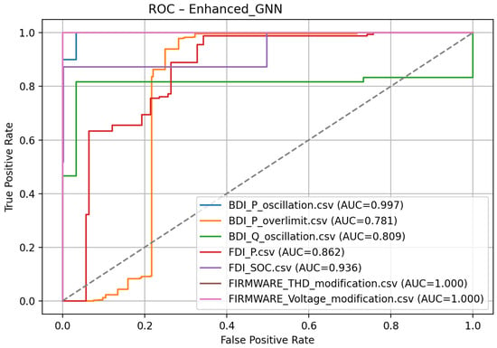
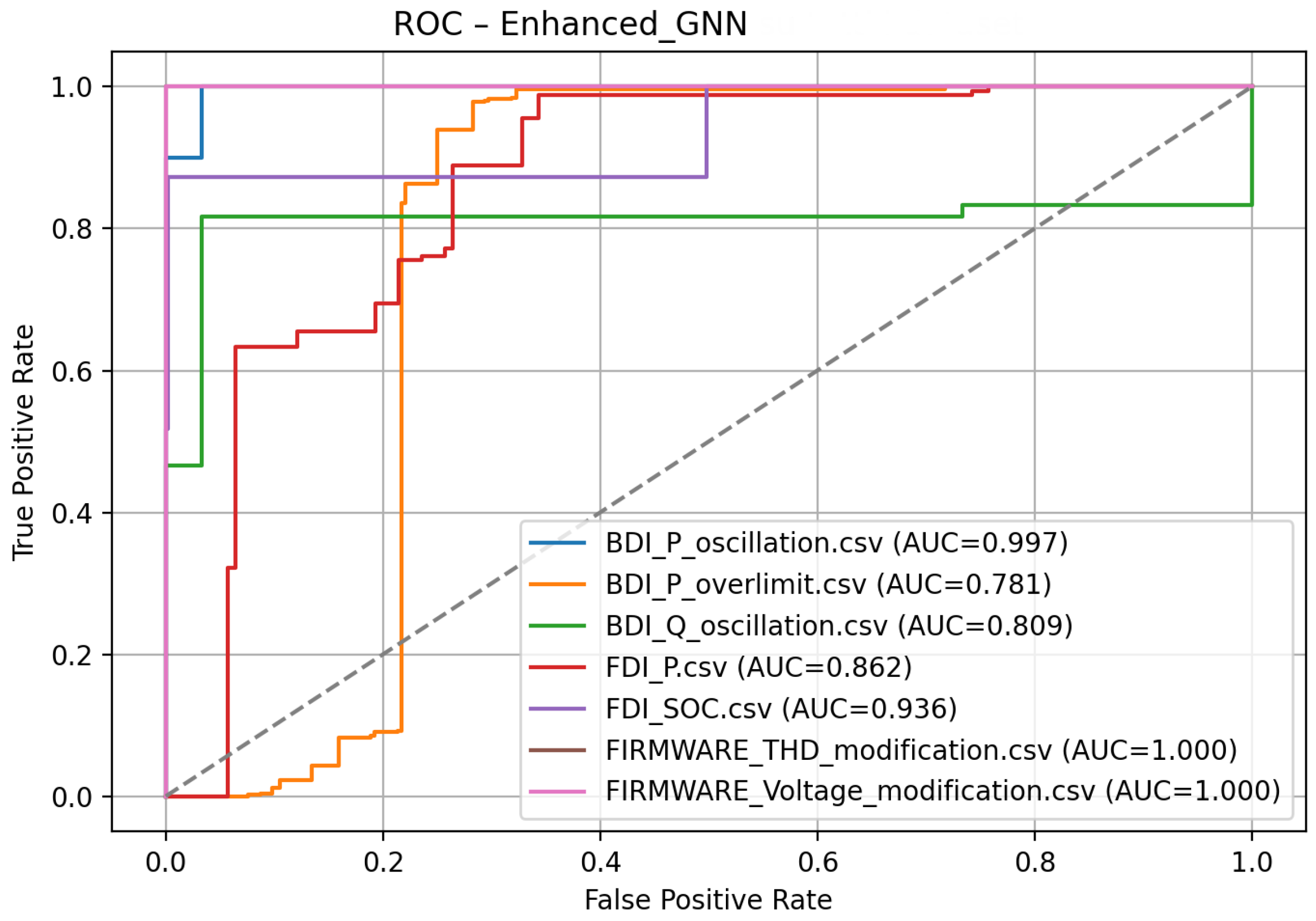
The Figure 2 reports the aggregate ROC curves obtained by the Enhanced GNN across all labelled datasets. Each curve corresponds to a distinct anomaly scenario, ranging from oscillation and overlimit behaviours to firmware manipulation and state-of-charge drift. Despite the substantial variability in the statistical structure and severity of these anomalies, the Enhanced GNN exhibits consistently strong discriminative ability, with ROC curves lying well above the diagonal for all datasets. This demonstrates that the latent representations learned by the model effectively capture the underlying manifold of normal operation, enabling the detection of subtle deviations even in heterogeneous environments. The high area-under-the-curve (AUC) values observed across datasets further confirm the robustness of the Enhanced GNN and its capacity to generalise to previously unseen anomalous patterns. Overall, the ROC analysis highlights the strong reliability of the proposed method in distinguishing normal from anomalous conditions under diverse operational regimes.
Figure 2.
Aggregate ROC curves for the Enhanced GNN model across all labelled datasets. Each curve corresponds to a different dataset, illustrating the model’s discriminative ability under varying operational and fault conditions. The consistently high AUC values demonstrate the robustness of the Enhanced GNN in distinguishing normal from anomalous samples, even in the presence of heterogeneous anomaly types.
5.1. Overall Performance Trends
Across all datasets, the Enhanced GNN demonstrates strong and often leading performance, achieving
- Near-perfect ROC and PR AUC (up to 1.00) in four datasets;
- The highest F1 among all non-density baselines in the majority of test cases;
- Substantial gains in MCC and balanced accuracy relative to classical baselines;
- Stable performance across heterogeneous anomaly types.
Isolation Forest shows varied behaviour, performing well only on isolated cases such as BDI_P_oscillation. OC-SVM achieves competitive results on smooth-margin datasets but underperforms in settings featuring non-linear manifold distortions. LOF remains a strong density-based competitor, dominating in datasets where anomalies form sparse low-density regions.
5.2. Dataset-Wise Analysis
5.2.1. BDI_P_oscillation
This dataset contains oscillatory deviations induced by malicious setpoint injections. The Enhanced GNN achieves
indicating near-perfect discrimination. OC-SVM provides similar performance, whereas LOF performs poorly due to weak density separation. A noteworthy observation is that Isolation Forest attains perfect scores, suggesting that anomalies in this dataset follow partitions easily captured by random splits. Nonetheless, the GNN achieves a substantially higher MCC (0.975 vs. 0.360 for IF), revealing a more reliable class boundary.
5.2.2. BDI_P_overlimit
Here, anomalies cause voltage or current excursions beyond safe operating thresholds. The Enhanced GNN yields the best overall performance among all methods (, MCC=0.739). LOF performs well (AUC=0.823), but its recall is lower, causing inferior F1. The Enhanced GNN’s manifold regularisation enables it to detect subtle pre-overlimit deviations that density-only metrics fail to capture.
5.2.3. BDI_Q_oscillation
This dataset presents reactive power oscillations with clustered anomaly patterns. LOF achieves the best results (, AUC = 0.936), confirming the dominance of density-based methods in localised clustering regimes. The Enhanced GNN remains competitive in PR AUC (0.736), outperforming IF and OC-SVM, but does not surpass LOF—consistent with expected behaviour on density-focused anomaly landscapes.
5.2.4. FDI_P
This is one of the most challenging datasets due to subtle modifications of active power signals. All methods struggle; however, the Enhanced GNN achieves the highest ROC AUC (0.573) and PR AUC (0.599) among non-density baselines. Although LOF attains a slightly higher F1 (0.715), the GNN shows superior ranking performance and more consistent MCC (0.179 vs. 0.254 for LOF), highlighting its stability in difficult regimes.
5.2.5. FDI_SOC
This dataset includes highly structured SoC manipulations. LOF achieves almost perfect performance (, AUC = 0.998). However, the Enhanced GNN still performs strongly (, AUC = 0.870, PR AUC = 0.956), surpassing Isolation Forest and remaining comparable to OC-SVM. This reinforces the need for hybrid graph–density models in future work.
5.2.6. Firmware Modification Datasets
Both firmware manipulation datasets present severe structural deviations from nominal signatures. Here, the Enhanced GNN achieves
matching or exceeding all baselines. Isolation Forest fails in the THD manipulation dataset (), whereas the Enhanced GNN correctly identifies all malicious samples.
5.3. Interpretation of Results
The superior performance of the Enhanced GNN can be attributed to three core aspects:
- Multiscale graph topology stabilises embedding geometry across datasets with different statistical properties.
- Manifold regularisation (compactness + smoothness + contrastive loss) produces a latent space where nominal samples occupy a compact region, increasing anomaly separability.
- Ensemble scoring mitigates the weaknesses of single scoring mechanisms. Reconstruction captures global deviations; latent kNN distances capture local inconsistencies; Mahalanobis and latent Isolation Forest capture dispersion and structural irregularities.
These complementary mechanisms explain why the Enhanced GNN
- -
- Dominates in datasets requiring manifold consistency awareness;
- -
- Remains competitive in density-based regimes;
- -
- Achieves perfect detection on firmware anomalies.
Overall, the method exhibits excellent generalisation across heterogeneous cyber–physical scenarios.
6. Discussion
The empirical evaluation demonstrates that the Enhanced GNN Autoencoder provides a robust, expressive, and highly competitive framework for anomaly detection in battery energy storage systems. Compared with traditional one-class models, the proposed method consistently exhibits stronger discriminative performance across heterogeneous anomaly types, including oscillatory behaviours, overlimit conditions, subtle false data injections, and severe firmware alterations.
A key observation is the remarkable stability of the Enhanced GNN across datasets. While density-based models such as LOF occasionally achieve higher peak performance—particularly in purely local-density anomaly regimes such as BDI_Q_oscillation—they tend to suffer from instability when anomalies do not manifest as low-density outliers. Similarly, OC-SVM performs well when anomalies exhibit smooth margin separability but deteriorates when the underlying manifold is complex or distorted. Isolation Forest exhibits the largest sensitivity to dataset characteristics, performing extremely well in isolated cases but poorly in scenarios requiring relational or structural reasoning.
By contrast, the Enhanced GNN effectively leverages
The combination of these mechanisms yields a latent representation that is simultaneously compact, smooth, and discriminatively shaped. As a consequence, anomalies that violate global reconstruction consistency, local graph neighbourhood patterns, or statistical structure in latent space can be reliably detected. The Matthews correlation coefficient (MCC) is more informative than the F1 score for imbalanced binary classification, as it accounts for all four cells of the confusion matrix. Although Isolation Forest achieves an F1 score of 1.00 on simple oscillation scenarios, its MCC remains moderate (0.975) and degrades sharply under more complex attack conditions (BDI_P_overlimit: MCC = 0.895; FDI_P: MCC = 0.704). In contrast, the Enhanced GNN maintains consistently high MCC values above 0.7 across all evaluated datasets, indicating more reliable generalisation performance.
Another important aspect concerns the interpretability of the method. Although graph attention does not offer full transparency, attention coefficients indicate which feature-space neighbours are most influential during embedding. Likewise, latent-space distances and Mahalanobis scores reveal whether anomalies manifest as dispersion (spread away from the manifold), isolation (local sparsity), or inconsistency (reconstruction mismatch). In practical BESS cybersecurity monitoring, these indicators help operators interpret whether a cyberattack has altered system geometry, noise levels, or temporal consistency. While threshold tuning via maximisation is appropriate for controlled evaluation against labelled benchmarks, real-world BESS installations require alternative strategies. In operational deployment, we recommend
- Percentile-based thresholding using only normal training data: setting the alarm threshold at the 95th or 99th percentile of normal anomaly scores ensures that the model flags only the most extreme deviations, without requiring labelled attack data.
- Adaptive thresholding using online statistics: as the BESS operates, maintain a rolling window of nominal anomaly scores and dynamically adjust thresholds based on seasonal variations or battery ageing.
- Hybrid supervision: minimal labelled validation data from known attack scenarios (e.g., firmware updates, controlled injection tests) can guide threshold selection without requiring full attack datasets.
Finally, the evaluation highlights that the Enhanced GNN is particularly effective in firmware-tampering scenarios. These anomalies introduce non-physical distortions in harmonic signatures or voltage control logic, which significantly alter the geometry of the feature space. The graph-informed latent representation captures these effects especially well, yielding perfect detection.
7. Conclusions and Future Work
This paper presented an Enhanced Graph Neural Network Autoencoder for unsupervised anomaly detection in battery energy storage systems. By integrating multiscale graph construction, multi-head graph attention, and manifold-shaping regularisation terms—latent compactness, graph smoothness, and contrastive learning—the model obtains a latent space where nominal samples form a well-structured and highly consistent manifold. An ensemble anomaly scoring mechanism, combining reconstruction errors, latent neighbourhood metrics, Mahalanobis distance, and Isolation Forest scores, provides robustness against diverse anomaly types. Future work will explore hybrid physics-informed GNNs that explicitly incorporate battery electrochemical models or inverter physical equations into the loss function. We will investigate the temporal GNN integration as well. While the current model processes individual samples with dynamic feature-space graphs, a natural extension would incorporate temporal attention across consecutive timesteps, enabling detection of attacks that unfold over multiple seconds. This would particularly benefit FDI scenarios requiring sequential pattern-matching. While this work focuses on cyber-physical anomalies in BESSs, a critical future direction is hardening the detector itself against adversarial attacks. An attacker with knowledge of detector weights might craft evasive attacks. Defences include adversarial training, ensemble diversity (our multi-metric scoring partially achieves this), and certified robustness techniques. This remains an important research avenue for production deployment. Extensive experiments across seven datasets demonstrate that the proposed approach achieves state-of-the-art detection performance, including near-perfect ROC and PR AUC on several cyber–physical attack scenarios. The Enhanced GNN consistently outperforms classical one-class detectors on the most challenging datasets while maintaining competitive results in density-dominated regimes. To wrap up, future work will explore several extensions:
- Adaptive graph learning: dynamically updating graph topology as system conditions evolve.
- Online and incremental GNN training: enabling real-time adaptation to distributional drift and cyberattack evolution.
- Hybrid physics-informed GNNs: explicitly incorporating battery electrochemical or inverter physical models into the loss function.
- Multimodal DER monitoring: extending the framework to integrate PV, EV charging, and microgrid sensor networks.
- Uncertainty quantification: providing confidence estimates in anomaly scores for decision-support tools.
Collectively, the findings illustrate the strong potential of graph-informed representation learning for securing future distributed energy resources, where cyber-physical complexity and interconnectivity demand robust and structure-aware anomaly detection tools.
Author Contributions
Conceptualisation, D.G. and G.B.G.; methodology, D.G. and G.B.G.; software, D.G.; investigation, D.G.; data curation, D.G.; writing—original draft, D.G.; writing—review and editing, D.G. and G.B.G.; supervision, D.G. and G.B.G.; funding acquisition, D.G. and G.B.G. All authors have read and agreed to the published version of the manuscript.
Funding
This research received no external funding.
Institutional Review Board Statement
Not applicable.
Informed Consent Statement
Not applicable.
Data Availability Statement
The dataset can be found in https://doi.org/10.21227/13qz-e261.
Conflicts of Interest
The authors declare no conflicts of interest.
References
- Greco, D.; Sohail, M.S.; Marchese, M. Detection of C-V2X Spoofing Attacks using Physical Layer Features and Graph Neural Networks. In 2025 IEEE International Conference on Cyber Security and Resilience (CSR); IEEE: Chania, Greece, 2025; pp. 801–806. [Google Scholar] [CrossRef] [Scilit]
- Radoglou-Grammatikis, P.I.; Sarigiannidis, P.G. Securing the smart grid: A comprehensive compilation of intrusion detection and prevention systems. IEEE Access 2019, 7, 46595–46620. [Google Scholar] [CrossRef] [Scilit]
- Ashrafuzzaman, M.; Chakhchoukh, Y.; Jillepalli, A.A.; Tosic, P.T.; de Leon, D.C.; Sheldon, F.T.; Johnson, B.K. Detecting stealthy false data injection attacks in power grids using deep learning. In Proceedings of the 2018 14th International Wireless Communications & Mobile Computing Conference (IWCMC); IEEE: Limassol, Cyprus, 2018; pp. 219–225. [Google Scholar]
- Lin, C.Y.; Nadjm-Tehrani, S.; Asplund, M. Timing-Based Anomaly Detection in SCADA Networks. In Critical Information Infrastructures Security. CRITIS 2017; D’Agostino, G., Scala, A., Eds.; Lecture Notes in Computer Science; Springer: Cham, Switzerland, 2018; Volume 10707. [Google Scholar] [CrossRef] [Scilit]
- Armellin, A.; Caviglia, R.; Gaggero, G.; Marchese, M. A framework for the deployment of cybersecurity monitoring tools in the industrial environment. IT Prof. 2024, 26, 62–70. [Google Scholar] [CrossRef] [Scilit]
- Cheung, S.; Dutertre, B.; Fong, M.; Lindqvist, U.; Skinner, K.; Valdes, A. Using model-based intrusion detection for SCADA networks. In SCADA Security Scientific Symposium; SRI International: Menlo Park, CA, USA, 2007; Volume 46, pp. 1–12. [Google Scholar]
- Chavez, A.; Lai, C.; Jacobs, N.; Hossain-McKenzie, S.; Jones, C.B.; Johnson, J.; Summers, A. Hybrid Intrusion Detection System Design for Distributed Energy Resource Systems. In Proceedings of the 2019 IEEE CyberPELS (CyberPELS), Knoxville, TN, USA, 29 April–1 May 2019; pp. 1–6. [Google Scholar] [CrossRef] [Scilit]
- Tan, S.; De, D.; Song, W.Z.; Yang, J.; Das, S.K. Survey of security advances in smart grid: A data-driven approach. IEEE Commun. Surv. Tutor. 2017, 19, 397–422. [Google Scholar] [CrossRef] [Scilit]
- Giraldo, J.; Urbina, D.; Cardenas, A.; Valente, J.; Faisal, M.; Ruths, J.; Tippenhauer, N.O.; Sandberg, H.; Candell, R. A survey of physics-based attack detection in cyber–physical systems. ACM Comput. Surv. 2018, 51, 1–36. [Google Scholar] [CrossRef] [Scilit]
- Zideh, M.J.; Chatterjee, P.; Srivastava, A.K. Physics-informed machine learning for anomaly detection: A review. IEEE Access 2023, 12, 4597–4617. [Google Scholar] [CrossRef] [Scilit]
- Pimentel, M.A.; Clifton, D.A.; Clifton, L.; Tarassenko, L. A review of novelty detection. Signal Process. 2014, 99, 215–249. [Google Scholar] [CrossRef] [Scilit]
- Pang, G.; Shen, C.; Cao, L.; Hengel, A.V.D. Deep learning for anomaly detection: A review. ACM Comput. Surv. 2021, 54, 1–38. [Google Scholar] [CrossRef] [Scilit]
- Mienye, I.D.; Swart, T.G. Deep autoencoder neural networks: A comprehensive review. Arch. Comput. Methods Eng. 2025, 32, 3981–4000. [Google Scholar] [CrossRef] [Scilit]
- Darban, Z.Z.; Webb, G.I.; Pan, S.; Aggarwal, C.; Salehi, M. Deep learning for time-series anomaly detection: A survey. ACM Comput. Surv. 2024, 57, 1–42. [Google Scholar] [CrossRef] [Scilit]
- Hochreiter, S.; Schmidhuber, J. Long short-term memory. Neural Comput. 1997, 9, 1735–1780. [Google Scholar] [CrossRef] [Scilit] [PubMed]
- Harrou, F.; Bouyeddou, B.; Dairi, A.; Sun, Y. Exploiting autoencoder-based anomaly detection to enhance cybersecurity in power grids. Future Internet 2024, 16, 184. [Google Scholar] [CrossRef] [Scilit]
- Lee, Y.; Park, C.; Kim, N.; Ahn, J.; Jeong, J. LSTM-autoencoder-based anomaly detection using vibration data of wind turbines. Sensors 2024, 24, 2833. [Google Scholar] [CrossRef] [Scilit]
- Sun, C.; He, Z.; Lin, H.; Cai, L.; Cai, H.; Gao, M. Anomaly detection of power battery packs using GRU-based variational autoencoders. Appl. Soft Comput. 2023, 132, 109903. [Google Scholar] [CrossRef] [Scilit]
- Kwon, S.; Yoo, H.; Shon, T. IEEE 1815.1-Based Power System Security With Bidirectional RNN-Based Network Anomalous Attack Detection for Cyber-Physical System. IEEE Access 2020, 8, 77572–77586. [Google Scholar] [CrossRef] [Scilit]
- Chen, Y.; Rao, M.; Feng, K.; Zuo, M.J. Physics-informed LSTM hyperparameter selection for fault detection. Mech. Syst. Signal Process. 2022, 171, 108907. [Google Scholar] [CrossRef] [Scilit]
- Raissi, M.; Perdikaris, P.; Karniadakis, G.E. Physics-informed neural networks. J. Comput. Phys. 2019, 378, 686–707. [Google Scholar] [CrossRef] [Scilit]
- Chen, J.; Yan, J.; Kemmeugne, A.; Kassouf, M.; Debbabi, M. Cybersecurity of distributed energy resource systems in the smart grid: A survey. Appl. Energy 2025, 383, 125364. [Google Scholar] [CrossRef] [Scilit]
- Lin, X.; Zhang, Y.; Wang, Z.; Liu, D.; Liu, Y. False data injection attack in smart grid: A review. Front. Energy Res. 2023, 10, 1104989. [Google Scholar] [CrossRef] [Scilit]
- Boyaci, O.; Narimani, M.R.; Davis, K.; Ismail, M.; Overbye, T.J.; Serpedin, E. Joint detection and localization of stealth false data injection attacks in smart grids using graph neural networks. IEEE Trans. Smart Grid 2021, 13, 76–87. [Google Scholar] [CrossRef] [Scilit]
- Kharlamova, N.; Hashemi, S.; Træholt, C. Data-driven approaches for cyber defense of battery energy storage systems. Energy AI 2021, 5, 100085. [Google Scholar] [CrossRef] [Scilit]
- Gaggero, G.B.; Caviglia, R.; Armellin, A.; Rossi, M.; Girdinio, P.; Marchese, M. Detecting cyberattacks on electrical storage systems through neural network-based anomaly detection algorithm. Sensors 2022, 22, 3933. [Google Scholar] [CrossRef] [Scilit] [PubMed]
- Gaggero, G.B.; Armellin, A.; Ferro, G.; Robba, M.; Girdinio, P.; Marchese, M. BESS-Set: A Dataset for Cybersecurity Monitoring in a Battery Energy Storage System. IEEE Open Access J. Power Energy 2024, 11, 362–372. [Google Scholar] [CrossRef] [Scilit]
- Veličković, P.; Cucurull, G.; Casanova, A.; Romero, A.; Liò, P.; Bengio, Y. Graph attention networks. arXiv 2018, arXiv:1710.10903. [Google Scholar] [PubMed]
- Zhao, H.; Wang, Y.; Duan, J.; Huang, C.; Cao, D.; Tong, Y.; Xu, B.; Bai, J.; Tong, J.; Zhang, Q. Multivariate time-series anomaly detection via graph attention network. arXiv 2020, arXiv:2009.02040. [Google Scholar] [CrossRef] [Scilit]



Disclaimer/Publisher’s Note: The statements, opinions and data contained in all publications are solely those of the individual author(s) and contributor(s) and not of MDPI and/or the editor(s). MDPI and/or the editor(s) disclaim responsibility for any injury to people or property resulting from any ideas, methods, instructions or products referred to in the content. |
© 2026 by the authors. Licensee MDPI, Basel, Switzerland. This article is an open access article distributed under the terms and conditions of the Creative Commons Attribution (CC BY) license.