A Lightweight Model for Power Quality Disturbance Recognition Targeting Edge Deployment

Abstract

To address the dual demands of accuracy and real-time performance in power quality disturbance (PQD) recognition for new power system, this paper proposes a lightweight model named the Cross-Channel Attention Three-Layer Convolutional Model (1D-CCANet-3), specifically designed for edge deployment. Based on the one-dimensional convolutional neural network (1D-CNN), the model features an ultra-compact architecture with only three convolutional layers and one fully connected layer. By incorporating a set of cross-channel attention (CCA) mechanisms in the final convolutional layer, the model further enhances disturbance recognition accuracy. Compared to other deep learning models, 1D-CCANet-3 significantly reduces computational and storage requirements for edge devices while achieving accurate and efficient PQD recognition. The model demonstrates robust performance in recognizing 10 types of PQD under varying signal-to-noise ratio (SNR) conditions. Furthermore, the model has been successfully deployed on the FPGA platform and exhibits high recognition accuracy and efficiency in real-world data validation. This work provides a feasible and effective solution for accurate and real-time PQD monitoring on edge devices in new power systems.

1. Introduction

With the large-scale integration of distributed renewable energy, the new power system is undergoing significant transformations [1]. Power quality disturbances (PQDs) in distribution networks have become more complex and unpredictable. PQD not only affects the performance and lifespan of power electronic devices but can also lead to severe accidents. Thus, accurate real-time monitoring of PQD signals is essential for ensuring the reliability and stability of power supply in new power systems [2].

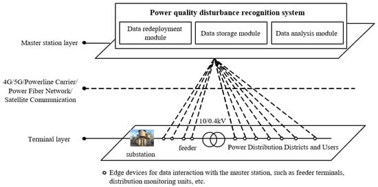
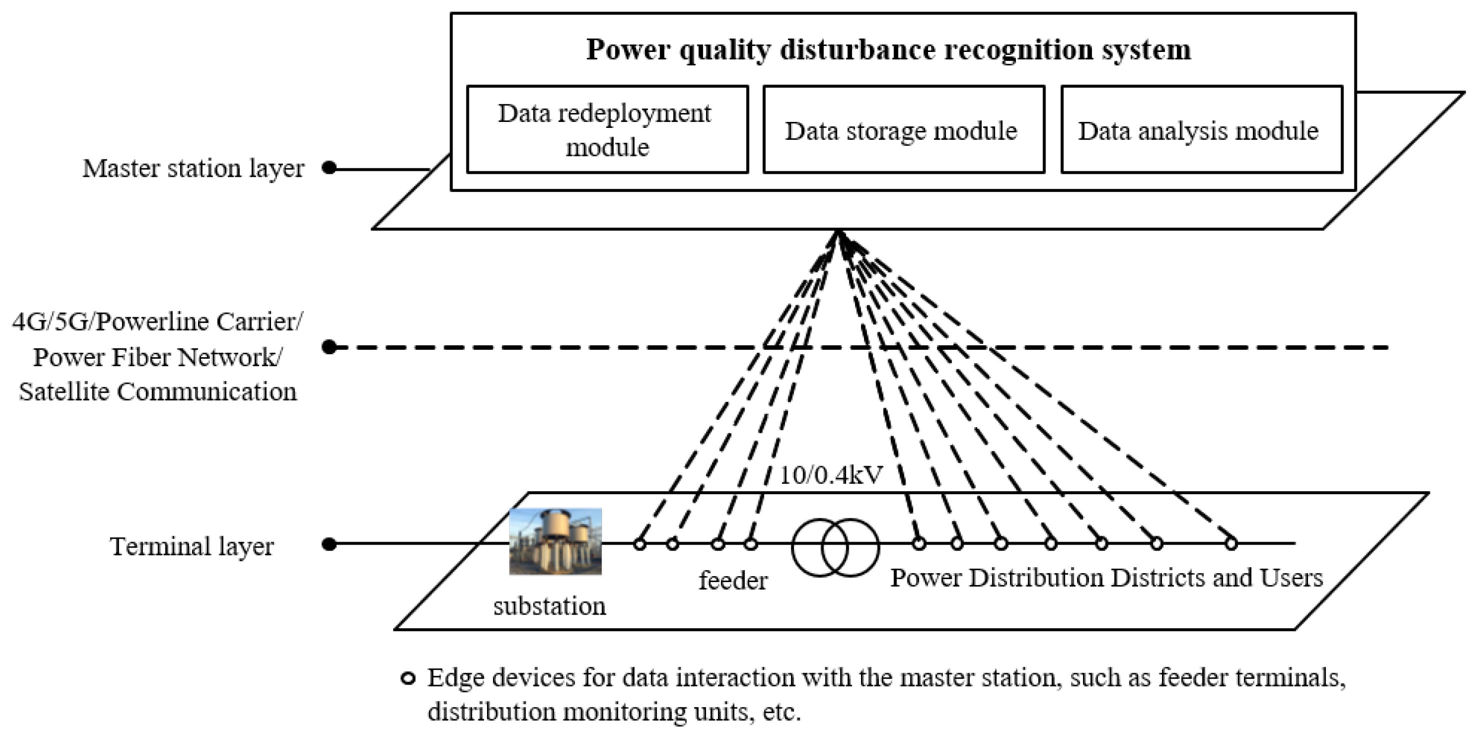
In current engineering applications, the typical architecture of PQD recognition systems is shown in Figure 1. Raw power quality data collected by edge devices at the terminal layer are transmitted to the master station via communication methods like 4G or fiber optics [3]. The master station layer, utilizing cloud platforms or central servers, processes the data centrally, leveraging its powerful computational and storage resources.

Figure 1. Architecture diagram of electric power quality disturbance recognition system.

However, as new power systems evolve, this centralized approach faces several challenges [4]. First, the increasing number of monitored nodes exponentially expands the data volume, creating storage burdens and hindering timely analysis. Second, limited communication bandwidth and transmission delays introduce high latency, making real-time monitoring difficult.

To address these challenges, computational tasks are delegated to edge devices deployed near the data source has become a novel approach for PQD recognition systems. Despite the extensive development and adoption of distributed intelligence in power grids over the past decade, shifting toward enhanced localized autonomy and decision-making efficiency. For complex tasks like Power Quality (PQ) monitoring, embedding deep learning directly onto edge hardware further advances this trajectory. This approach facilitates substantial computational offloading from the master station and enables real-time, high-dimensional feature extraction at the data source [5], ensuring deterministic performance for localized PQ recognition.

Methods for PQD recognition are broadly categorized into traditional signal processing-based methods and deep learning-based methods [6].

Traditional methods use signal processing techniques like Fourier Transform (FT) [7], Wavelet Transform (WT) [8], S-Transform (ST) [9], and Hilbert Transform (HT) [10] to convert time-domain signals and extract features. These features are then classified by algorithms such as Support Vector Machines (SVM) [11], Decision Trees (DT) [12], or Extreme Learning Machines (ELM) [13]. While effective for single disturbance events, these methods struggle with feature extraction and recognition accuracy for complex and dynamic disturbances in modern power systems.

Deep learning methods, with their powerful learning and nonlinear feature mapping capabilities, address these challenges, offering a promising approach to improving recognition accuracy [14].

To meet the demands for accuracy and real-time performance in new power system, research is increasingly focused on deploying deep learning models at the edge [15]. However, in resource-constrained environments with diverse devices, selecting suitable model architectures and efficiently deploying large-scale models remain critical challenges in PQD recognition [16].

Deep learning methods for PQD recognition fall into two categories: image-based recognition and fully end-to-end recognition.

Image-based methods integrate traditional signal processing with high-performance deep learning algorithms [17], converting one-dimensional signals into two-dimensional images for feature extraction and classification [18]. Ref. [19] proposed a method combining discrete wavelet transform (DWT) with multi-resolution analysis (MRA) and a deep convolutional neural network (DCNN) to compress raw signals and automatically learn features for PQD classification. Ref. [20] extended this idea by using Markov transition fields (MTF) to convert 1D PQD signals into 2D images rich in texture, followed by an improved DenseNet to extract multi-scale visual features, showing robustness for complex disturbance types. Ref. [21] investigated the application of vision transformers (ViT) for PQD classification, where 1D signals are transformed into time-frequency images using smoothed pseudo Wigner–Ville distribution (SPWVD) before ViT-based classification. While these methods offer advantages in accuracy and generalization, their high resource demands limit practical use on edge devices [22]. The additional signal conversion steps increase computational complexity, requiring more processing power, storage, and energy [23].

In contrast, fully end-to-end methods rely on neural networks, such as 1D CNNs [24], RNNs [25] or DFAN [26], to directly process and classify raw time-series signals. Ref. [27] develops a Transformer-based end-to-end classifier for PQD, inputting raw voltage sequences without dedicated feature extraction. Ref. [28] integrates a 1D convolutional branch for temporal features and a Transformer branch for frequency domain global dependencies, fused via a cross-attention mechanism. This design directly processes raw PQD time series, jointly learning representations and classification in a unified model. By eliminating signal processing and dimensional conversion, these methods significantly reduce computational demands, making them more suitable for resource-constrained edge environments [29].

This paper focuses on the integration of deep learning-based Power Quality Disturbance(PQD) recognition algorithm into edges hardware devices. As local data processing units, these edge devices not only minimize response latency but also facilitate computational offloading from the master station, mitigating centralized storage and processing bottlenecks to ensure deterministic real-time performance. When coupled with deep learning architectures optimized for high-throughput identification, this framework guarantees a synergy of operational efficiency and diagnostic precision in power quality monitoring [30]. The main contributions are as follows:

(1) Four evaluation metrics—model size, GPU memory usage, computational complexity, and inference time—are introduced to analyze model resource consumption. Additionally, the Edge-Deployment Suitability Score (EDSS) is proposed to evaluate model suitability for edge deployment.

(2) Representative RNN and 1D CNN models are compared in terms of PQD recognition performance, highlighting their advantages and limitations for edge deployment.

(3) A lightweight PQD recognition model, 1D-CCANet-3, based on 1D CNN, is proposed for edge deployment.

(4) Extensive experiments demonstrate that the proposed model significantly reduces resource requirements while maintaining high recognition accuracy across various SNR levels.

(5) The proposed model is successfully deployed on an FPGA platform for real-time validation. Testing with real-world data confirms its high accuracy and efficiency, proving its practicality for edge deployment in PQD monitoring.

This paper is structured as follows: Section 1 introduces the study. Section 2 discusses edge deployment and evaluation metrics. Section 3 examines PQD generation and fully end-to-end recognition methods. Section 4 details the proposed algorithm. Section 5 compares the algorithm with other models and includes a deployment validation experiment. Section 6 concludes the paper.

2. Overview of Edge Deployment

2.1. Introduction to Edge Intelligence

The edge devices designed for deployment are located at the Point of Common Coupling (PCC), which serves as the critical demarcation point between the utility grid and the customer-side installations. By measuring this point, the devices can monitor the power quality of an entire feeder using a minimal number of sensors and effectively assess the impact of customer-side disturbances, significantly reducing the total cost of system ownership compared to individual customer-side monitoring and facilitating faster localized decision-making.

With the rapid development of digital networks, edge devices are evolving to include basic information analysis and processing capabilities, reducing reliance on centralized cloud servers and improving network transmission efficiency. Local data processing on edge devices helps address challenges like latency, bandwidth limitations, and real-time decision-making.

Edge intelligence, which focuses on deploying deep learning models on edge devices, enables real-time perception, inference, and response, providing faster and smarter solutions [31].

However, deploying deep learning models on edge devices presents challenges, including limited computational and storage resources, energy constraints, and the complexity of diverse model architectures across different applications.

To address these challenges, four research directions have emerged: model compression and optimization, model partitioning, edge-cloud collaboration, and lightweight model design. These approaches aim to reduce the computational and storage burdens on edge devices while improving model efficiency and adaptability.

Model compression and optimization [32] use techniques like pruning and quantization to reduce model size and computational complexity, making models more suitable for edge devices.

Model partitioning [33] involves dividing a model into segments, executing different parts on different resources, reducing edge device load while maintaining performance.

Edge-cloud collaboration [34] creates a cooperative framework between edge devices and cloud servers, enabling seamless training and inference alternation between the two.

Lightweight model design [35] optimizes deep learning models to fit the limited resources of edge devices while maintaining real-time performance and low power consumption, ensuring adaptability across various applications.

This paper adopts a lightweight model design approach to balance real-time performance and accuracy in PQD recognition, ensuring applicability to resource-constrained edge devices in distribution networks.

2.2. Model Resource Consumption Metrics

Resource constraints are a primary challenge when deploying deep learning models on edge devices. This paper evaluates model resource utilization using four metrics: model size, GPU memory usage, computational complexity, and inference time. Additionally, a comprehensive metric, the Edge-Deployment Suitability Score (EDSS), is introduced to assess model suitability for edge deployment, combining recognition accuracy and the four metrics mentioned.

2.2.1. Model Size

Model size refers to the number of parameters in the model (Params). Larger models enhance representational capacity but require more storage and loading resources. Smaller models reduce storage usage and ease deployment, making them suitable for resource-constrained environments.

2.2.2. GPU Memory Usage

GPU memory usage measures the memory consumed during a single forward propagation. It reflects storage requirements for intermediate variables in edge devices with limited memory. Lower memory usage ensures smooth operation. The unit used is megabytes (MB).

2.2.3. Computational Complexity

Computational complexity measures the operations required for forward propagation. This paper uses Multiply-Accumulate Operations (MACs) as the metric. Lower complexity indicates fewer computational resources, improving real-time performance.

2.2.4. Inference Time

Inference time measures the time for a single forward propagation. Shorter inference times indicate higher efficiency, ensuring the model meets real-time requirements. The unit used is milliseconds (ms).

2.2.5. Edge-Deployment Suitability Score

EDSS quantifies the suitability of deep learning models for edge devices. It considers recognition accuracy, model size, GPU memory usage, computational complexity, and inference time. The formula for calculating EDSS is shown in (1).

$$\begin{array}{cc}\hfill EDSS& =\mathrm{Accuracy}·\left(w_1·N_{\mathrm{Params}}+w_2·N_{\mathrm{GPU} \mathrm{Memory}}+w_3·N_{\mathrm{MACs}}+w_4·N_{\mathrm{Inf} \mathrm{time}}\right).\hfill \end{array}$$

(1)

where $w_1$, $w_2$, $w_3$, and $w_4$ are weights (0.3, 0.2, 0.3, and 0.2, respectively), and the normalized values for resource consumption metrics are represented in (2). Specifically, model size and GPU memory usage primarily measure the storage resource consumption, while computational complexity and inference time focus more on the consumption of computational resources during inference. Considering that storage and computational resources are of comparable importance in practical FPGA deployment environments, a total weight of 0.5 was assigned to each category in (1). Within their respective domains, model size and computational complexity are the core metrics that directly determine storage utilization and real-time inference capability, representing the primary bottlenecks for deployment feasibility. In contrast, memory footprint and inference latency can often be partially mitigated through subsequent hardware optimization strategies. Consequently, a higher proportion of weight was allocated to model size and computational complexity to highlight their critical significance in practical deployment scenarios.

$$N_{\mathrm{Metric}}={\displaystyle \frac{\mathrm{Max}\mathrm{Metric}-\mathrm{Metric}\mathrm{for}\mathrm{Model}}{\mathrm{Max}\mathrm{Metric}-\mathrm{Min}\mathrm{Metric}}}.$$

(2)

As shown in (1), the maximum value of EDSS is 1, and a higher EDSS indicates a model’s higher suitability for edge deployment.

3. End-to-End Recognition Model

3.1. Mathematical Model of PQD Signals

According to IEEE Std 1159-2019 [36], power quality disturbances are classified into seven types: voltage sag (C1), voltage swell (C2), voltage interruption (C3), transient impulse (C4), transient oscillation (C5), harmonics (C6), and voltage flicker (C7). Based on international standards and models from literature [24], this paper presents mathematical models for eight power quality disturbances, including the standard signal (C0) with negligible disturbances. The parameter equations and variation ranges for these disturbances are provided in Table 1.

Table 1. Equation for Single Disturbance Parameter of Electric Power Quality $({\omega }_0=2\pi ·50, T=0.02\mathrm{s})$.

Labels	Types	Parameter Equation	Range of Parameter Variations
C0	standard signal	$y\left(t\right)=\{1+\alpha [u(t-t_1)-u(t-t_2)]\}·sin\left({\omega }_{0}t\right)$	$-0.1\le \alpha \le 0.1,T\le t_2-t_1\le 9T$
C1	voltage sag	$y\left(t\right)=\{1-\alpha [u(t-t_1)-u(t-t_2)]\}·sin\left({\omega }_{0}t\right)$	$0.1\le \alpha \le 0.9,T\le t_2-t_1\le 9T$
C2	voltage swell	$y\left(t\right)=\{1+\alpha [u(t-t_1)-u(t-t_2)]\}·sin\left({\omega }_{0}t\right)$	$0.1\le \alpha \le 0.8,T\le t_2-t_1\le 9T$
C3	voltage interruption	$y\left(t\right)=\{1-\alpha [u(t-t_1)-u(t-t_2)]\}·sin\left({\omega }_{0}t\right)$	$0.9\le \alpha \le 1.0,T\le t_2-t_1\le 9T$
C4	transient impulse	$y\left(t\right)=\alpha [u(t-t_1)-u(t-t_2)]+sin\left({\omega }_{0}t\right)$	$1\le \alpha \le 3,0.05T\le t_2-t_1\le 0.15T$
C5	transient oscillation	$$\begin{gathered} y\left(t\right)=\alpha ·exp\left(-(t-t_1)/\tau \right)·sin\left(2\pi f_n(t-t_1)\right)· \\ [u(t-t_1)-u(t-t_2)]+sin\left({\omega }_{0}t\right) \end{gathered}$$	$$\begin{gathered} 0.1\le \alpha \le 0.8, 150\le \tau \le 1000, \\ 300\le f_n\le 900, 0.05T\le t_2-t_1\le 3T \end{gathered}$$
C6	harmonics	$$\begin{gathered} y\left(t\right)= \\ {\alpha }_{1}sin\left(w_{0}t\right)+{\alpha }_{3}sin\left(3w_{0}t\right)+{\alpha }_{5}sin\left(5w_{0}t\right)+{\alpha }_{7}sin\left(7w_{0}t\right) \end{gathered}$$	$0.05\le {\alpha }_1,{\alpha }_3,{\alpha }_7\le 0.15,\sum {\alpha }_i^2=1$
C7	voltage flicker	$y\left(t\right)=\left[1+\alpha sin\left(\beta w_{0}t\right)\right]·sin\left(w_{0}t\right)$	$0.1\le \alpha \le 0.2,0.1\le \beta \le 0.5$

In the new power system, complex structures often lead to composite disturbances, where multiple disturbance types occur simultaneously. To better reflect practical scenarios, this paper simulates eight single disturbances and two composite disturbances (voltage sag with harmonics, C8, and voltage swell with harmonics, C9) using MATLAB. The ten disturbance types are encoded using a One-Hot encoding scheme.

3.2. Comparison of End-to-End Recognition Models

Due to the limited computational and storage resources of edge devices, this paper avoids converting one-dimensional time-series data into images for recognition. This decision saves resources on edge devices and eliminates the need for complex 2D convolutional networks. Instead, we focus on a fully end-to-end method, which reduces computational load and storage requirements.

The fully end-to-end approach includes two types: RNN and 1D CNN. In this paper, Long Short-Term Memory (LSTM) networks and a modified one-dimensional ResNet-18 (1D-ResNet-18) are chosen as representatives. Experiments on the same GPU chip evaluate the recognition performance of these models on 10 types of PQD signals (C0–C9). The recognition accuracies for various signal-to-noise ratios (SNRs) ranging from 30 to 50 dB are shown in Table 2.

Table 2. Accuracy of Recognizing Different Disturbance Types by Two Models.

Types	LSTM	1D-ResNet-18
C0	99.5%	99.9%
C1	99.4%	98.9%
C2	99.0%	99.6%
C3	99.7%	100.0%
C4	100.0%	100.0%
C5	99.7%	99.7%
C6	100.0%	100.0%
C7	100.0%	100.0%
C8	100.0%	100.0%
C9	99.9%	100.0%
Average accuracy	99.72%	99.81%

As shown in Table 2, both the LSTM and 1D-ResNet-18 models achieve high recognition accuracy for all 10 disturbance signal types. Notably, the recognition accuracy for transient impulse (C4), harmonics (C6), voltage flicker (C7), and composite disturbance (C8) reaches 100%.

Both models exhibit excellent recognition performance on a GPU chip, making either suitable depending on the specific requirements. However, for edge device deployment, it is crucial to evaluate the resource consumption during forward propagation and the complexity of the model architecture.

The resource consumption for a single forward pass of the LSTM and 1D-ResNet-18 models is shown in Table 3. For the LSTM model, the hidden state dimension is set to 128, and the number of layers is 2.

Table 3. Resource Consumption for One Forward Propagation of Two Models.

Evaluation Metrics	Comparison Model
	LSTM	1D-ResNet-18
Model size/Params	200,458	3,847,114
GPU memory usage	0.314 MB	2.034 MB
Computational complexity	128.780 × ${10}^6$	109.604 × ${10}^6$
Inference time	8.601 ms	2.941 ms
EDSS	0.4986	0.4991

As shown in Table 3, the EDSS of LSTM is 0.4986, indicating that it is not well-suited for edge deployment. The high computational complexity and longer inference time of the LSTM model, due to its step-by-step processing of sequences and complex gated operations, make it less efficient for real-time applications.

The EDSS of 1D-ResNet-18 is 0.4991, slightly higher than LSTM, but still not ideal for edge deployment due to its high number of parameters and GPU memory usage. Relying on external storage for resource management increases inference time and negatively impacts real-time performance.

Compared to RNN, 1D CNN models like 1D-ResNet-18 are more efficient in utilizing edge device resources, thanks to their simpler, parallelizable convolutional layers. Therefore, this paper focuses on optimizing 1D CNN for better real-time performance and proposes a lightweight PQD recognition model more suitable for edge deployment.

4. The Cross-Channel Attention Three-Layer Convolutional Neural Network (1D-CCANet-3)

4.1. Basic Principles and Structure of 1D CNN

1D CNN is an extension of the Convolutional Neural Network, specifically designed for one-dimensional sequential data. Its core idea stems from the convolution operation, which captures local features in the input sequence, allowing the model to better understand the structure and patterns of time-series data. 1D CNNs consist primarily of convolutional layers, activation function layers, pooling layers, and fully connected layers.

4.1.1. Convolutional Layer

The convolutional layer (Conv1D) is the core component of 1D CNN. It slides the convolution kernel over the input sequence to effectively capture local features. The key parameters, such as stride and padding, influence how the model processes the input sequence, enabling the network to autonomously learn important features for subsequent tasks. The one-dimensional convolution operation with multiple input channels is defined in

$$Y[c,t]=\sum _{i=0}^{C_{\mathrm{in}}-1}\sum _{a=0}^{k-1}X[i,t+a]·W[c,i,a]+b\left[c\right].$$

(3)

where $Y[c,t]$ represents the output at time step t for the c-th channel, $X[i,t+a]$ is the input at time step $t+a$ for the i-th channel, $W[c,i,a]$ is the weight for the convolution kernel, and $b\left[c\right]$ is the bias term. $C_{\mathrm{in}}$ denotes the number of input channels, and k is the kernel size.

4.1.2. Activation Function Layer

Activation functions in 1D CNN introduce non-linearity, enabling the network to learn complex patterns. Common functions like ReLU, Sigmoid, Tanh, and Softmax are used. ReLU, as in (4), is preferred in edge device deployment due to its efficiency in addressing the vanishing gradient problem and its simple computation. The Softmax function, as in (5), used in multi-class classification, converts outputs into probability distributions.

$$\mathrm{ReLU}\left(x\right)=max(0,x).$$

(4)

$$P_i={\displaystyle \frac{exp\left(z_i\right)}{{\sum }_{j=1}^{N}exp\left(z_j\right)}}.$$

(5)

4.1.3. Pooling Layer

The pooling layer in 1D CNN reduces feature dimensionality, lowering computational complexity and memory usage, crucial for hardware deployment. Max Pooling, commonly used in PQD recognition, selects the maximum value in each pooling window, preserving key features. The operation is defined by stride s and kernel size k, where the output at position i is given by (6).

$$Y\left[i\right]=max\left(X\right[i·s:(i·s+k)\left]\right).$$

(6)

4.1.4. Fully Connected Layer

In 1D CNN, the fully connected (FC) layer links all neurons from the previous layer to the current one. It transforms feature maps from convolutional layers into the final output. The FC layer can be viewed as a special convolutional layer with a kernel size covering the entire input, stride $s=1$, and no weight sharing. While capable of learning complex feature representations, the FC layer has many parameters, making it prone to overfitting and unsuitable for edge deployment. Thus, its use in PQD recognition should be optimized based on task complexity and dataset characteristics.

4.2. The Architecture of the 1D-CCANet-3 Model

To optimize resource utilization on edge devices and enhance model compatibility, this paper proposes a PQD recognition model based on a 1D CNN structure. Drawing inspiration from the classic LeNet-5 architecture, a cross-channel adaptive attention (CCA) mechanism is integrated to address the issues of excessive parameters and deep layers in the 1D-ResNet-18 model. This design prioritizes simplicity, minimizing computational and storage demands for edge devices.

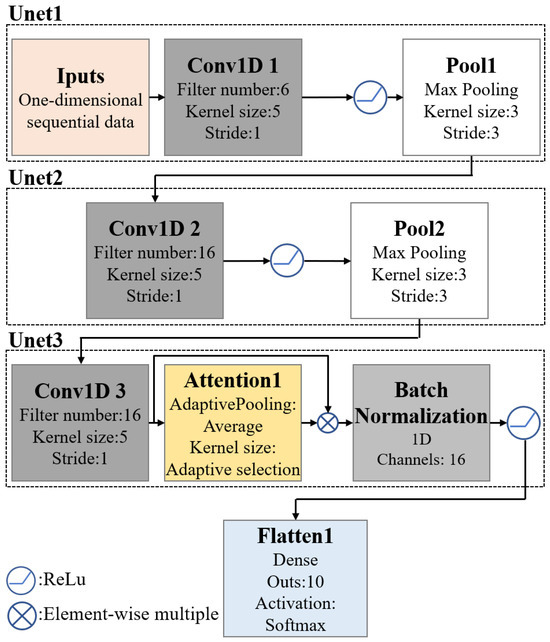
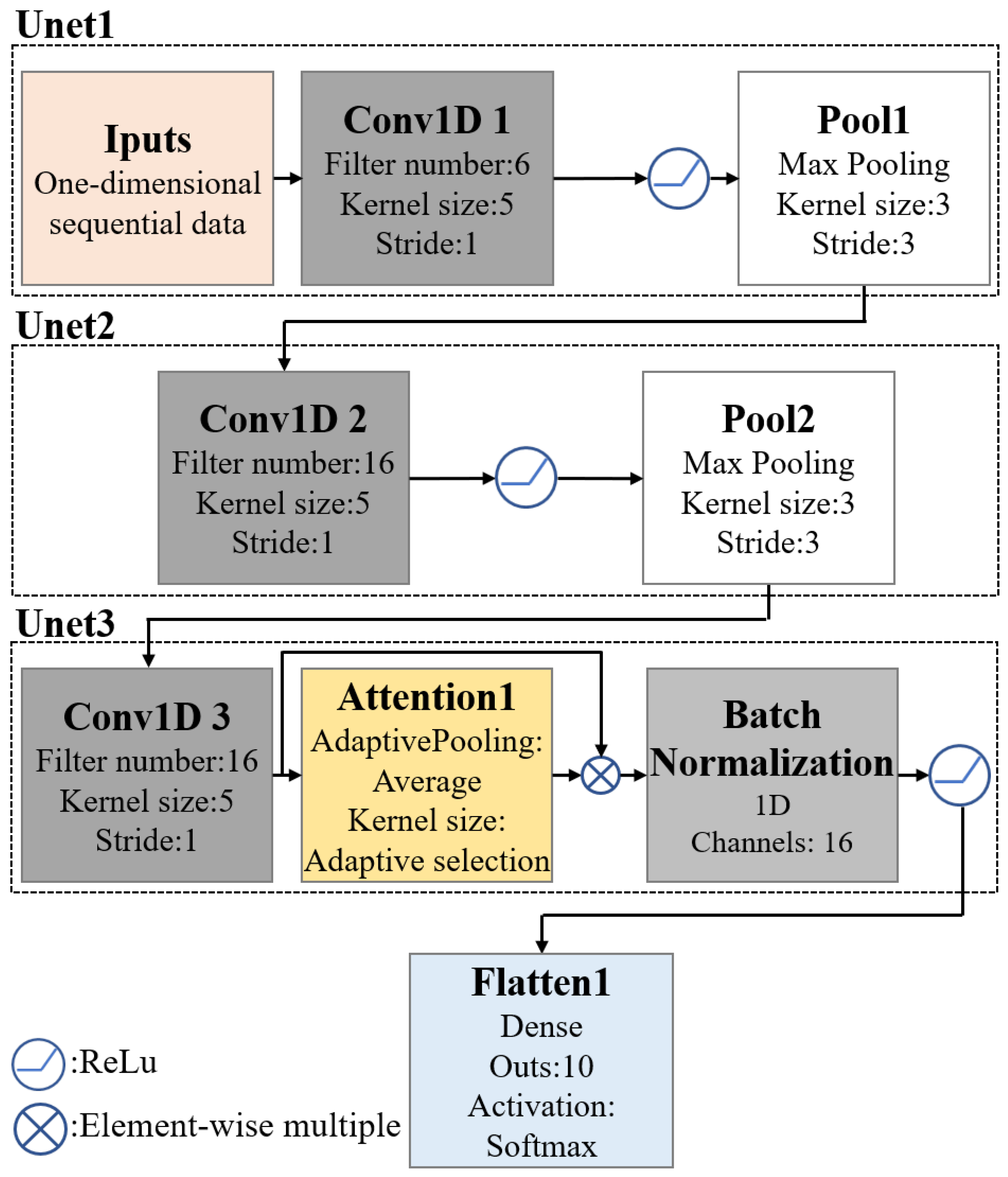
Compared with 2-layer and 4-layer architectures, the 3-layer configuration provides the optimal balance between feature depth and hardware resource consumption. The architecture of the proposed 1D-CCANet-3 model is shown in Figure 2.

Figure 2. Structure diagram of the Cross-Channel Attention Three-Layer Convolutional Neural Network (1D-CCANet-3).

The LeNet-5 model consists of three convolutional layers and two fully connected layers. As shown in Figure 2, the proposed recognition model retains the three convolutional layers of LeNet-5 but optimizes the fully connected layers to reduce parameters and computational complexity. A CCA module and a Batch Normalization (BN) layer are added after the third convolutional layer for enhanced feature extraction.

To facilitate edge deployment, the CCA mechanism is adapted from the Efficient Channel Attention Network (ECANet) [37], which is computationally efficient and ideal for processing one-dimensional time-series feature sequences of PQD.

The CCA module first applies channel average pooling to extract representative feature scales, then uses one-dimensional convolution to capture cross-channel relationships. Weight information from the neighborhood features is reloaded to improve the generalization of effective features. In PQD recognition, this mechanism enables the model to adjust feature weights based on their relevance, allowing it to focus on key information critical for identifying disturbances and improving recognition performance.

The BN layer is introduced to accelerate the model’s training process and improve convergence speed. In combination with the attention mechanism, the BN layer enhances the model’s sensitivity and accuracy when handling complex and variable PQD data, thereby optimizing the streamlined architecture proposed in this paper.

A comparison of network parameters between the 1D-LeNet-5 model and the proposed recognition model is shown in Table 4, where it is assumed that the input PQD signal has a size of (1, 640).

Table 4. The Comparison of Network Parameters between 1D-LeNet-5 and 1D-CCANet-3.

	1D-LeNet-5			1D-CCANet-3
	Layers	Outputs	Params	Layers	Outputs	Params
Unet1	Conv1D-1	(6, 636)	30	Conv1D-1	(6, 636)	30
	Pool1	(6, 212)	-	Pool1	(6, 212)	-
Unet2	Conv1D-2	(16, 208)	480	Conv1D-2	(16, 208)	480
	Pool2	(16, 69)	-	Pool2	(16, 69)	-
Unet3	Conv1D-3	(120, 65)	9600	Conv1D-3	(16, 65)	1280
	Reshape	Maxpooling: 120		Attention + BN	(16, 65)	35
Dense	FC1	84	10,080	Reshape	Flatten: 1040
	FC2	10	840	FC1	10	10,400
Total	-	-	21,030	-	-	12,225

As shown in Table 4, the overall architecture of the 1D-CCANet-3 model is similar to that of the 1D-LeNet-5 model. After three convolutional layers, an adaptive attention module is added to capture cross-channel information. The fully connected layer is used only once for classification output.

To balance resource consumption and classification performance, 1D-CCANet-3 reduces the output channels of Conv1D-3 and removes the pooling layer from Unet3. After processing with the CCA mechanism and BN layer, the multi-channel output of Conv1D-3 is flattened into a one-dimensional feature sequence, which is then input into the fully connected layer for classification.

As shown in Table 4, compared to the 1D-LeNet-5 model, the 1D-CCANet-3 model reduces the number of parameters by about 42%, lowering resource requirements for edge deployment. The addition of the CCA mechanism and BN layer introduces only a small increase in parameters, significantly improving recognition performance without greatly increasing model complexity.

5. Example Analysis

5.1. PQD Dataset Generation

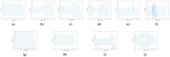
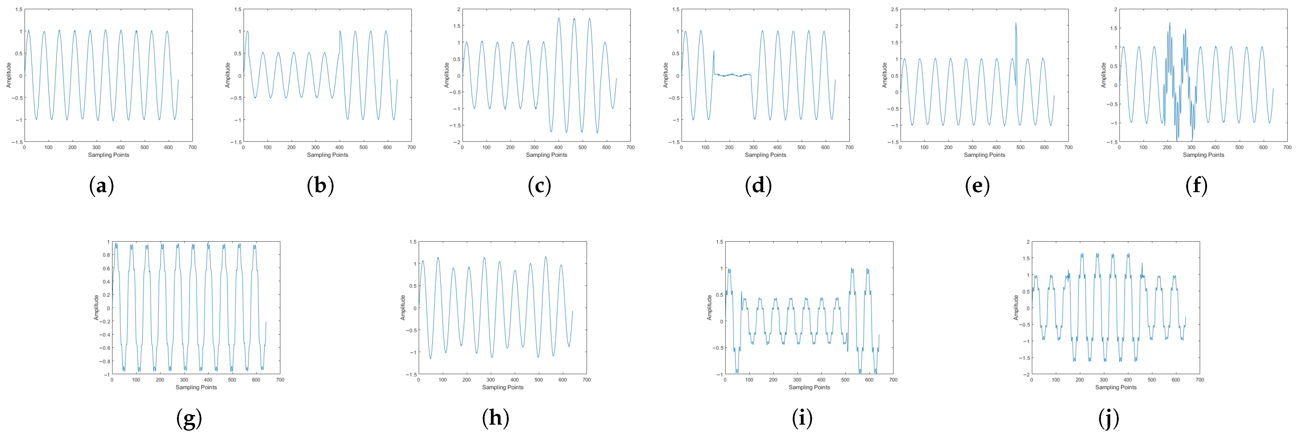
Based on the PQD mathematical models in Table 1, samples of 10 types of PQD signals are generated. The sampling frequency is 3.2 kHz, capturing 64 points per cycle, with sampling performed every 10 cycles, resulting in 640 data points. The simulated waveforms of the disturbances are shown in Figure 3. For each disturbance type, 5000 training samples and 1000 validation samples are generated. To account for noise in real-world sampling, Gaussian white noise with an SNR between 30 dB and 50 dB is randomly added to each disturbance during simulation.

Figure 3. The waveforms of the 10 types of disturbances. (a) C0 standard signal; (b) C1 voltage sag; (c) C2 voltage swell; (d) C3 voltage interruption; (e) C4 transient impulse; (f) C5 transient oscillation; (g) C6 harmonics; (h) C7 voltage flicker; (i) C8 voltage sag with harmonics; (j) C9 voltage swell with harmonics.

5.2. Models Training

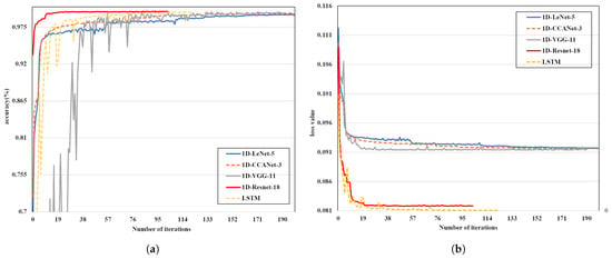
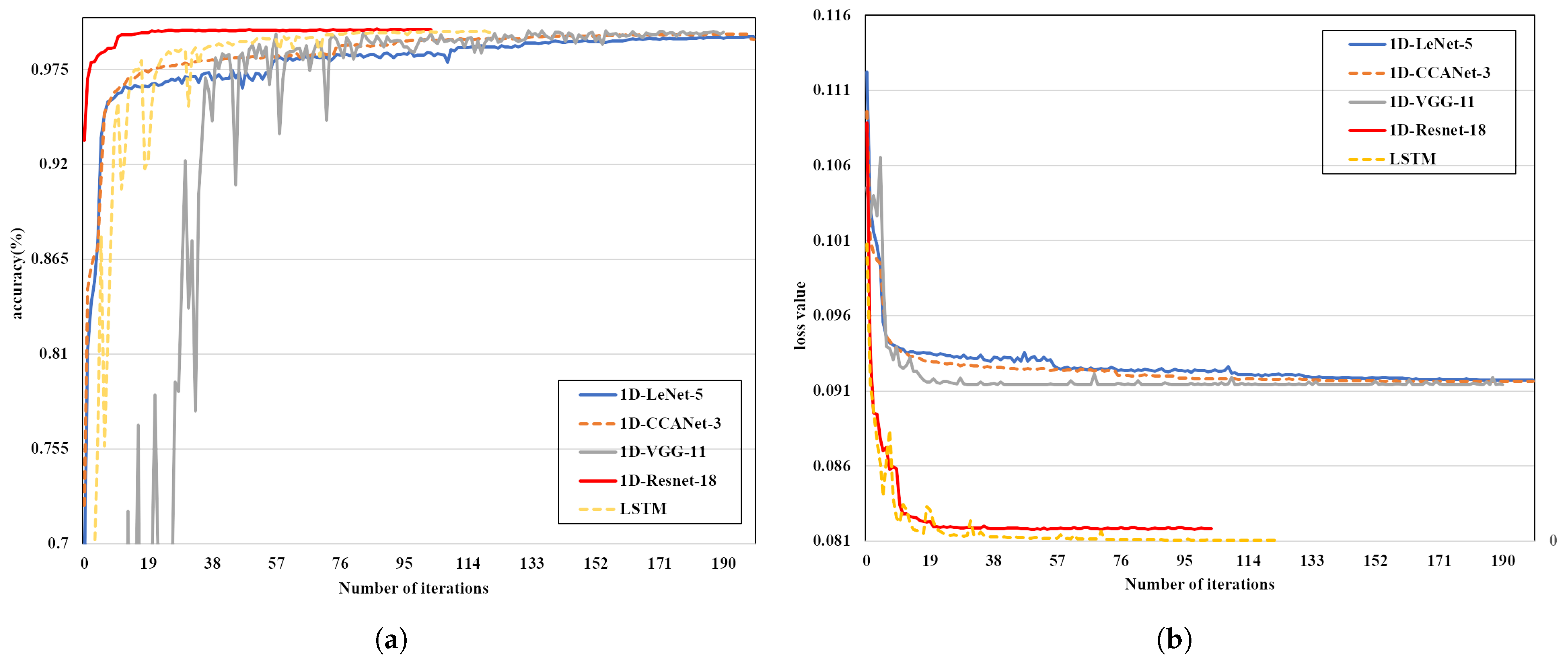
The simulated PQD data is normalized and then fed into the 1D-CCANet-3 model for training. The model’s performance is compared with that of 1D-LeNet-5, 1D-VGG-11, 1D-ResNet-18, and LSTM models. The accuracy and loss curves during training are shown in Figure 4.

Figure 4. Accuracy curve of model training and loss curve. (a) Accuracy curves. (b) Loss curve.

The training parameters are as follows: learning rate of 0.001, Adam optimizer, batch size of 16, and 200 iterations. To prevent overfitting, the learning rate is reduced by 50% if the loss does not decrease for 10 consecutive iterations. Training terminates if the loss does not decrease after 20 iterations.

From the loss curve in Figure 4b, all five models converge quickly, with training curves stabilizing after about 20–40 iterations, maintaining high recognition accuracy. Among them, 1D-ResNet-18 converges the fastest, completing training after 104 iterations, followed by the LSTM model at 124 iterations. The 1D-VGG-11 model converges slightly slower, entering a slow convergence phase around the 40th iteration. Both 1D-LeNet-5 and 1D-CCANet-3 models did not terminate early, but their recognition accuracy continued to rise, loss decreased, and training curve fluctuations diminished, indicating improved stability and eventual convergence.

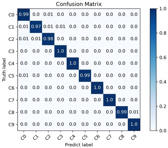
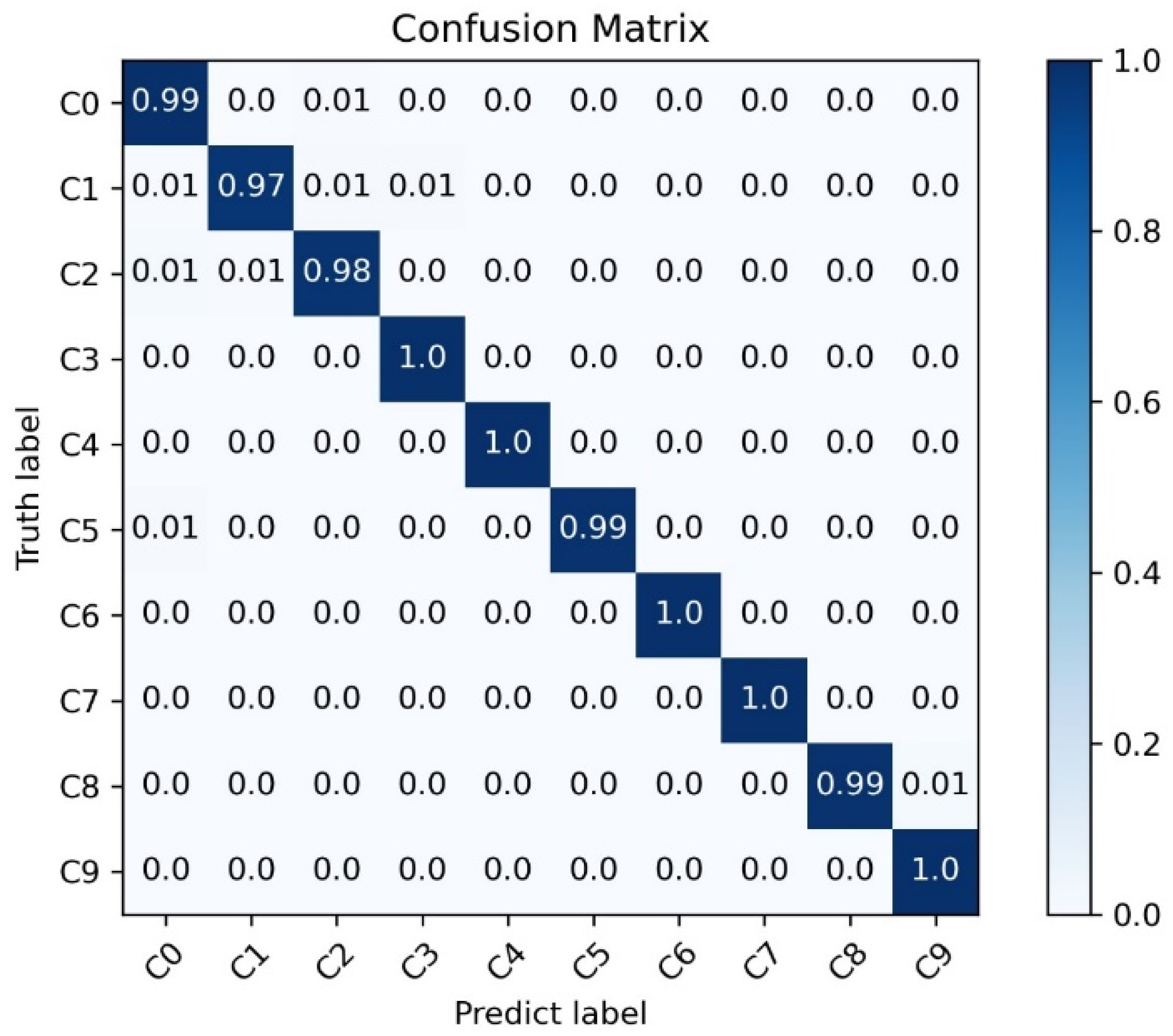
The accuracy curve in Figure 4a shows that, after convergence, the 1D-CCANet-3 model’s recognition accuracy is lower than that of LSTM and 1D-ResNet-18 but remains high, comparable to 1D-VGG-11. The recognition accuracy of 1D-CCANet-3 for the 10 types of power quality disturbances in the training set is shown in the confusion matrix in Figure 5.

Figure 5. The classification performance of the proposed model 1D-CCANet-3.

Although the lightweight model 1D-CCANet-3 exhibits a slightly higher loss, it achieves a superior trade-off between classification accuracy and resource consumption. The lower loss of LSTM and ResNet-18 comes at the cost of significantly higher parameter counts and computational latency. For edge devices, these models exceed the optimal resource budget.

In the confusion matrix shown in Figure 5, rows represent the model’s classification results, and columns represent the actual disturbance types. From Figure 5, it can be seen that the 1D-CCANet-3 model achieved over 97% accuracy for all 10 types of power quality disturbances. Specifically, the recognition accuracy for voltage interruption (C3), transient impulse (C4), harmonics (C6), voltage flicker (C7), and composite disturbances (C9) reached 100%. These results demonstrate that the 1D-CCANet-3 model performs excellently in classifying all 10 types of PQD signals.

5.3. Model Noise Robustness and Resource Consumption Comparison

To further evaluate the effectiveness of the proposed method for PQD recognition, the recognition accuracy of different models on PQD test sets with SNRs of 30 dB, 40 dB, 50 dB, and no noise was compared to assess the noise robustness of the model [38]. The comparison results are shown in Table 5.

Table 5. The Classification Performance of Different Models under Various SNRs.

SNRs	Accuracy/%
	Ours	1D-LetNet-5	1D-VGG-11	LSTM	1D-ResNet-18
30 dB	99.11	98.54	99.15	99.13	99.28
40 dB	99.40	99.16	99.40	99.75	99.70
50 dB	99.52	99.12	99.49	99.78	99.66
No noise	99.60	99.16	99.57	99.83	99.69
Average	99.41	99.00	99.40	99.62	99.58

From Table 5, the proposed method demonstrates varying advantages and disadvantages in recognition accuracy and noise robustness compared to the other models. As noise increases, the recognition accuracy of the 1D-CCANet-3 model decreases, but it still achieves 99.11% accuracy under 30 dB noise.

In all noise conditions, 1D-CCANet-3 outperforms the 1D-LeNet-5 model and performs similarly to the 1D-VGG-11 model under high noise levels. However, LSTM and 1D-ResNet-18 show better performance.

The results indicate that the 1D-CCANet-3 model maintains good classification performance across different SNRs. Additionally, the resource consumption of the models is compared to highlight the advantages of the 1D-CCANet-3 model for edge deployment, with results shown in Table 6.

Table 6. The Resource Consumption of Different Models.

Models	Evaluation Metrics
	Model Size/Params	GPU Memory Usage	Comp. Complexity	Inference Time	EDSS
Ours	12,225	0.102 MB	0.215 × ${\mathbf{10}}^{\mathbf{6}}$	0.489 ms	0.9941
1D-LetNet-5	21,030	0.146 MB	0.754 × ${10}^6$	0.532 ms	0.9839
1D-VGG-11	236,155	2.462 MB	236.155 × ${10}^6$	2.098 ms	0.4402
LSTM	200,458	0.314 MB	128.78 × ${10}^6$	8.601 ms	0.6015
1D-ResNet-18	3,847,114	2.034 MB	109.604 × ${10}^6$	2.941 ms	0.3353

As shown in Table 6, the 1D-CCANet-3 model has the highest EDSS value, close to 1, indicating its superior suitability for edge deployment compared to other models. The 1D-CCANet-3 model further reduces storage and computational resource requirements for edge devices compared to the 1D-LeNet-5 model. It also has significantly lower computational complexity than the other three models, resulting in much shorter inference times—only 23.31%, 5.685%, and 16.63% of the times for 1D-VGG-11, LSTM, and 1D-ResNet-18, respectively.

In conclusion, the 1D-CCANet-3 model offers excellent recognition performance, noise robustness, and efficient resource usage during inference, making it highly suitable for real-time, accurate PQD classification on edge devices.

5.4. Experimental Deployment and Validation on FPGA Platform

To validate the feasibility and performance of the 1D-CCANet-3 model in real-world scenarios, it is deployed on a Field-Programmable Gate Array (FPGA) platform, specifically the Xilinx Kintex-7 410T (K7-410T) chip, which offers ample logic resources, memory capacity, and DSP units.

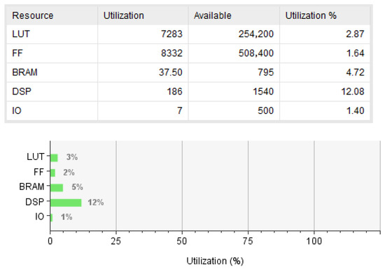
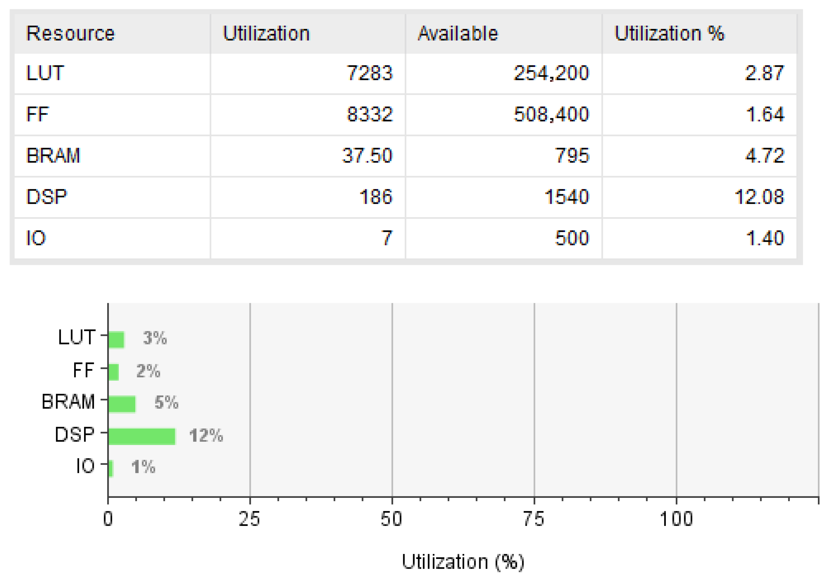
The model is quantized to 16-bit fixed-point to reduce resource consumption, and a deployment strategy involving full parallelism within the convolutional kernel and input channels is used to reduce latency and improve hardware utilization. The hardware implementation is completed using Verilog on the VIVADO platform, generating a configuration file for direct loading onto the FPGA. Resource consumption after deployment is shown in Figure 6.

Figure 6. The resource utilization of the 1D-CCANet-3 model after deployment.

As shown in Figure 6, DSP resources are the most consumed, accounting for only 12.08%, indicating the model’s relatively low resource demand. This suggests that the deployment strategy can be further optimized to reduce inference time by allocating more resources.

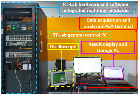
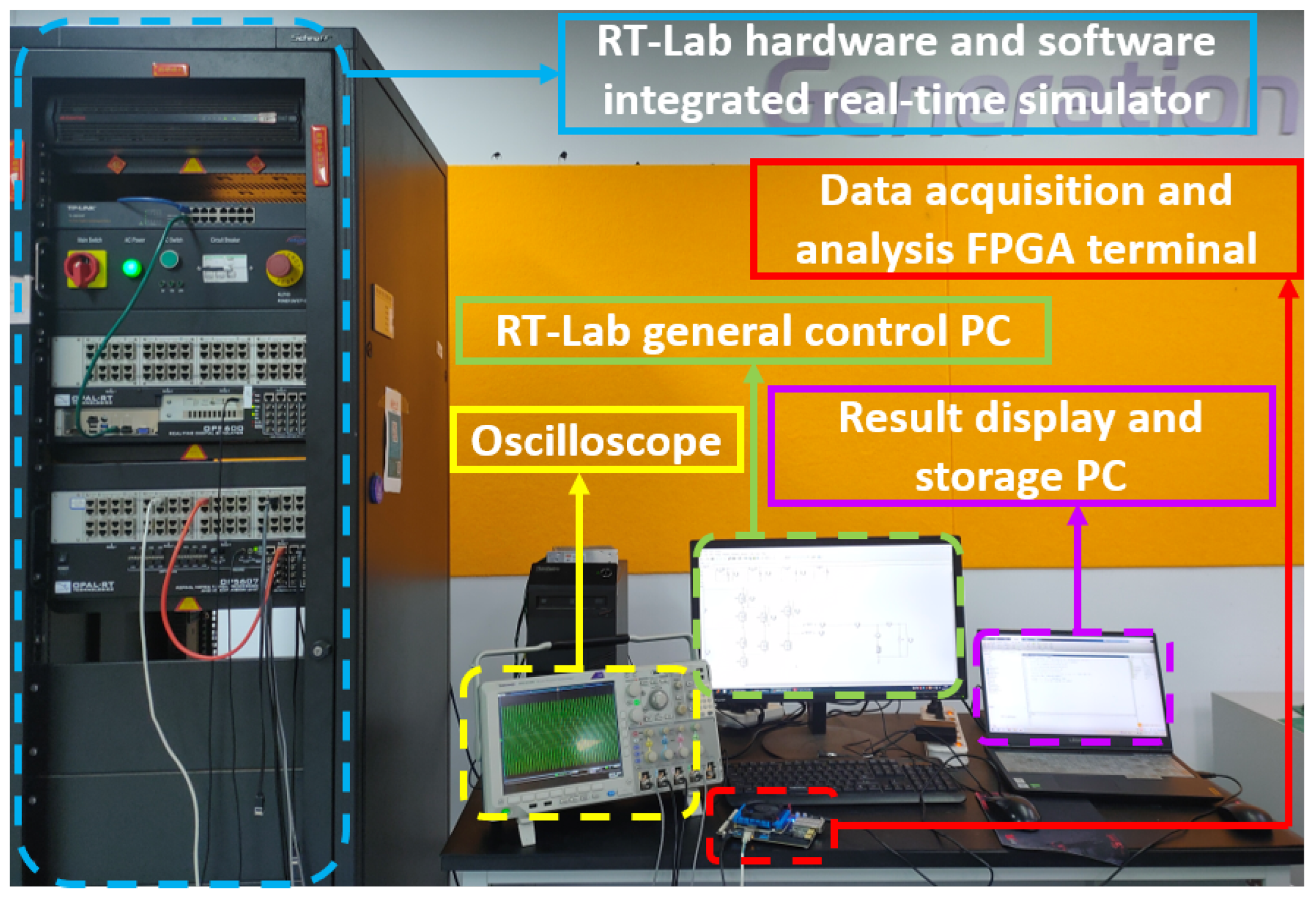
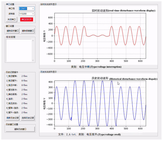
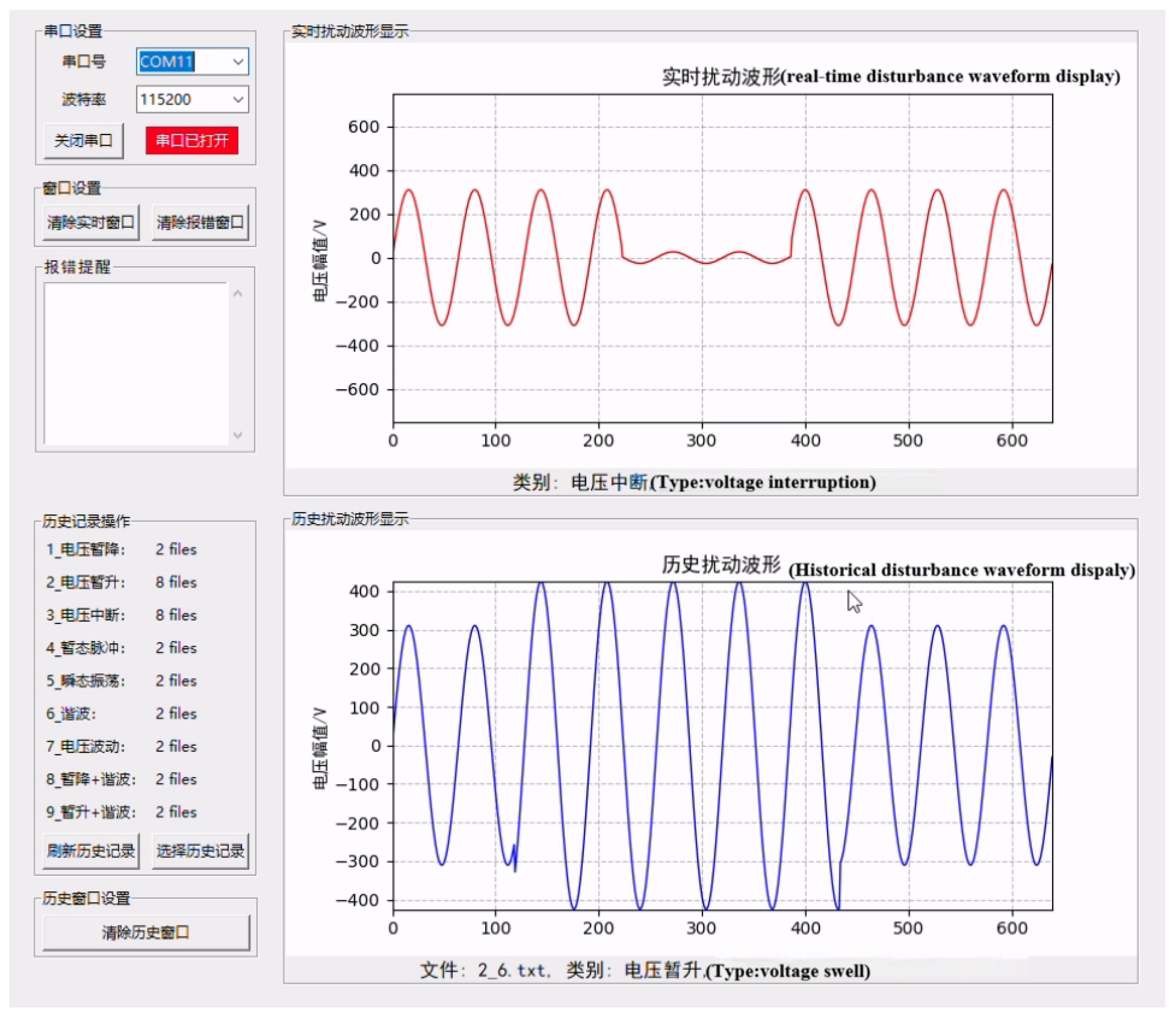
Additionally, a real-data verification platform was built using the FPGA, consisting of RT-Lab, FPGA, Personal Computer (PC), and an oscilloscope, as shown in Figure 7. RT-Lab generates the actual PQD data, the oscilloscope monitors waveform changes, and the FPGA performs data sampling and real-time disturbance recognition. The recognition results are transmitted to the PC for displaying and recording, the PC visualization window is shown in Figure 8, which demonstrates that not only can accurately receive and display real-time disturbance data from the FPGA, but also verifies that the model, once deployed on the FPGA processing board, performs inference and prediction correctly with robust operational stability.

Figure 7. Physical Diagram of FPGA-based Real Data Verification Platform.

Figure 8. The PC visualization window for displaying and recording the recognition results.

For validation, 50 sets of data are generated for each type of PQD, and the results are shown in Table 7. The model maintains high recognition accuracy in real-world scenarios, validating the effectiveness and reliability of the 1D-CCANet-3 model.

Table 7. The Results of the Verification Experiment.

Types	Samples	Correct	Accuracy (%)
C0	50	50	100.0
C1	50	48	96.0
C2	50	49	98.0
C3	50	50	100.0
C4	50	50	100.0
C5	50	48	96.0
C6	50	50	100.0
C7	50	49	98.0
C8	50	50	100.0
C9	50	50	100.0
Total	500	494	98.8

6. Conclusions

In response to the dual demands for both accuracy and real-time performance in PQD recognition at the edge of the new power systems, this paper proposes the lightweight intelligent recognition model, 1D-CCANet-3, based on one-dimensional convolutional neural networks. Experimental results demonstrate that the model’s lightweight design reduces its size by at least 42%, while maintaining high recognition accuracy and robustness to noise. This makes it highly suitable for deployment on low-cost edge devices with limited computational resources. The streamlined architecture not only significantly eases the model’s transferability across different platforms but also offers the potential for further optimization of computational complexity and reduction in inference time, tailored to the specific computational characteristics of various edge devices. This flexibility ensures that the model can meet the edge-end devices’ requirements for accurate classification and real-time monitoring of PQD in the new power system. Additionally, the proposed model’s efficiency and performance highlight its practical feasibility and advantage in real-world edge deployment scenarios.

References

- Babayomi, O.; Zhang, Z.; Dragicevic, T.; Hu, J.; Rodriguez, J. Smart grid evolution: Predictive control of distributed energy resources—A review. Int. J. Electr. Power Energy Syst. 2023, 147, 108812. [Google Scholar] [CrossRef] [Scilit]
- Chawda, G.S.; Shaik, A.G.; Shaik, M.; Padmanaban, S.; Holm-Nielsen, J.B.; Mahela, O.P.; Kaliannan, P. Comprehensive review on detection and classification of power quality disturbances in utility grid with renewable energy penetration. IEEE Access 2020, 8, 146807–146830. [Google Scholar] [CrossRef] [Scilit]
- Azmi, K.H.M.; Radzi, N.A.M.; Azhar, N.A.; Samidi, F.S.; Zulkifli, I.T.; Zainal, A.M. Active electric distribution network: Applications, challenges, and opportunities. IEEE Access 2022, 10, 134655–134689. [Google Scholar] [CrossRef] [Scilit]
- Khalid, M. Smart grids and renewable energy systems: Perspectives and grid integration challenges. Energy Strategy Rev. 2024, 51, 101299. [Google Scholar] [CrossRef] [Scilit]
- Xu, H.; Seng, K.P.; Ang, L.M.; Smith, J. Decentralized and distributed learning for AIoT: A comprehensive review, emerging challenges, and opportunities. IEEE Access 2024, 12, 101016–101052. [Google Scholar] [CrossRef] [Scilit]
- Rizeakos, V.; Bachoumis, A.; Andriopoulos, N.; Birbas, M.; Birbas, A. Deep learning-based application for fault location identification and type classification in active distribution grids. Appl. Energy 2023, 338, 120932. [Google Scholar] [CrossRef] [Scilit]
- Khetarpal, P.; Tripathi, M.M. A critical and comprehensive review on power quality disturbance detection and classification. Sustain. Comput. Inform. Syst. 2020, 28, 100417. [Google Scholar] [CrossRef] [Scilit]
- Fu, L.; Yan, K.; Zhu, T. PowerCog: A practical method for recognizing power quality disturbances accurately in a noisy environment. IEEE Trans. Ind. Inform. 2022, 18, 3105–3113. [Google Scholar] [CrossRef] [Scilit]
- Liu, M.; Chen, Y.; Zhang, Z.; Deng, S. Classification of power quality disturbance using segmented and modified S-transform and DCNN-MSVM hybrid model. IEEE Access 2023, 11, 890–899. [Google Scholar] [CrossRef] [Scilit]
- Kaushik, R.; Mahela, O.P.; Bhatt, P.K.; Khan, B.; Padmanaban, S.; Blaabjerg, F. A hybrid algorithm for recognition of power quality disturbances. IEEE Access 2020, 8, 229184–229200. [Google Scholar] [CrossRef] [Scilit]
- Zhou, Q.; Zhang, S.; Li, Y.; Li, Z.; Fang, Q.; Huang, H. Disturbance classification method for microgrids based on EEMD-Transformer-SVM. IEEE Access 2023, 11, 78934–78944. [Google Scholar] [CrossRef] [Scilit]
- Shams, N.; Wall, P.; Terzija, V. Active power imbalance detection, size and location estimation using limited PMU measurements. IEEE Trans. Power Syst. 2019, 34, 1362–1372. [Google Scholar] [CrossRef]
- Subudhi, U.; Dash, S. Detection and classification of power quality disturbances using GWO ELM. J. Ind. Inf. Integr. 2021, 22, 100204. [Google Scholar] [CrossRef] [Scilit]
- Beniwal, R.K.; Saini, M.K.; Nayyar, A.; Qureshi, B.; Aggarwal, A. A critical analysis of methodologies for detection and classification of power quality events in smart grid. IEEE Access 2021, 9, 83507–83534. [Google Scholar] [CrossRef] [Scilit]
- Massaoudi, M.; Abu-Rub, H.; Refaat, S.S.; Chihi, I.; Oueslati, F.S. Deep Learning in smart grid technology: A review of recent advancements and future prospects. IEEE Access 2021, 9, 54558–54578. [Google Scholar] [CrossRef] [Scilit]
- Shuvo, M.M.H.; Islam, S.K.; Cheng, J.; Morshed, B.I. Efficient acceleration of deep learning inference on resource-constrained edge devices: A review. Proc. IEEE 2023, 111, 42–91. [Google Scholar] [CrossRef] [Scilit]
- Cui, C.; Duan, Y.; Hu, H.; Wang, L.; Liu, Q. Detection and classification of multiple power quality disturbances using stockwell transform and deep learning. IEEE Trans. Instrum. Meas. 2022, 71, 2519912. [Google Scholar] [CrossRef] [Scilit]
- Wang, J.; Wang, Z.; Zhang, D. Power Quality Disturbance Classification Based on Recursive Graph and Pre-Trained Transfer Learning. South. Power Syst. Technol. 2025, 19, 48–56+114. [Google Scholar]
- Li, D.; Channa, I.A.; Chen, X.; Dou, L.; Khokhar, S.; Ab Azar, N. A new deep learning method for classification of power quality disturbances using DWT-MRA in utility smart grid. Comput. Electr. Eng. 2024, 117, 109290. [Google Scholar] [CrossRef] [Scilit]
- Zhou, L.; Gu, S.; Liu, Y.; Zhu, C. A novel recognition method for complex PQDs based on MTF and improved DenseNet. Front. Energy Res. 2024, 12, 1328994. [Google Scholar]
- Anwar, M.H.; Baig, M.M.A.; Shaikh, A.J.; Abro, A.G. Detection and classification of power quality disturbances: Vision transformers vs. CNN. Aims Energy 2025, 13, 1052–1075. [Google Scholar] [CrossRef] [Scilit]
- Wang, X.; Han, Y.; Leung, V.C.M.; Niyato, D.; Yan, X.; Chen, X. Convergence of edge computing and deep learning: A comprehensive survey. IEEE Commun. Surv. Tuts. 2020, 22, 869–904. [Google Scholar] [CrossRef] [Scilit]
- Wang, F.; Zhang, M.; Wang, X.; Ma, X.; Liu, J. Deep learning for edge computing applications: A state-of-the-art survey. IEEE Access 2020, 8, 58322–58336. [Google Scholar]
- Wang, S.; Chen, H. A novel deep learning method for the classification of power quality disturbances using deep convolutional neural network. Appl. Energy 2019, 235, 1126–1140. [Google Scholar] [CrossRef] [Scilit]
- Xiao, X.; Li, K. Multi-Label classification for power quality disturbances by integrated deep learning. IEEE Access 2021, 9, 152250–152260. [Google Scholar] [CrossRef] [Scilit]
- Liu, Y.; Su, X.; Liu, K.; Han, J.; Zhang, W.; Guo, H.; Wang, S. Method for Identifying Composite Power Quality Disturbances Based on Deep Frequency Attention Network. South. Power Syst. Technol. 2025, 19, 143–151+172. [Google Scholar]
- Saber, A.M.; Youssef, A.; Svetinovic, D.; Zeineldin, H.; Kundur, D.; El-Saadany, E. Enhancing Power Quality Event Classification with AI Transformer Models. In Proceedings of the 2024 IEEE Power & Energy Society General Meeting (PESGM), Seattle, WA, USA, 21–25 July 2024; pp. 1–5. [Google Scholar]
- Wang, T.; Zhuo, J.; Hou, Y.; Lu, Z.; Li, Y. Power quality disturbance classification via a time-frequency feature-fused transformer model with cross-attention mechanism. Electr. Power Syst. Res. 2026, 251, 112330. [Google Scholar] [CrossRef] [Scilit]
- Younesi, A.; Ansari, M.; Fazli, M.; Ejlali, A.; Shafique, M.; Henkel, J. A comprehensive survey of convolutions in deep learning: Applications, challenges, and future trends. IEEE Access 2024, 12, 41180–41218. [Google Scholar] [CrossRef] [Scilit]
- Feng, D. Embedded parallel computing platform for real-time recognition of power quality disturbance based on deep network. Teh. Vjesn. 2023, 30, 1920–1928. [Google Scholar]
- Xu, D.; Li, T.; Li, Y.; Su, X.; Tarkoma, S.; Jiang, T.; Crowcroft, J.; Hui, P. Edge intelligence: Empowering intelligence to the edge of network. Proc. IEEE 2021, 109, 1778–1837. [Google Scholar] [CrossRef] [Scilit]
- Choudhary, T.; Mishra, V.; Goswami, A.; Sarangapani, J. A comprehensive survey on model compression and acceleration. Artif. Intell. Rev. 2020, 53, 5113–5155. [Google Scholar] [CrossRef] [Scilit]
- Li, H.; Li, X.; Fan, Q.; He, Q.; Wang, X.; Leung, V.C.M. Distributed DNN inference with fine-grained model partitioning in mobile edge computing networks. IEEE Trans. Mobile Comput. 2024, 23, 9060–9074. [Google Scholar] [CrossRef] [Scilit]
- Yao, J.; Zhang, S.; Yao, Y.; Wang, F.; Ma, J.; Zhang, J.; Chu, Y.; Ji, L.; Jia, K.; Shen, T.; et al. Edge-Cloud polarization and collaboration: A comprehensive survey for AI. IEEE Trans. Knowl. Data Eng. 2023, 35, 6866–6886. [Google Scholar] [CrossRef] [Scilit]
- Chen, F.; Li, S.; Han, J.; Ren, F.; Yang, Z. Review of lightweight deep convolutional neural networks. Arch. Comput. Methods Eng. 2024, 31, 1915–1937. [Google Scholar] [CrossRef] [Scilit]
- IEEE Standard 1159-2009; IEEE Recommended Practice for Monitoring Electric Power Quality. IEEE: New York, NY, USA, 2009.
- Wang, Q.; Wu, B.; Zhu, P.; Li, P.; Zuo, W.; Hu, Q. ECA-Net: Efficient channel attention for deep convolutional neural networks. In Proceedings of the 2020 IEEE/CVF Conference on Computer Vision and Pattern Recognition (CVPR), Seattle, WA, USA, 14–19 June 2020; pp. 11531–11539. [Google Scholar]
- Xi, X.; Xing, C.; Qin, R.; Guo, C.; Zhou, X. Power Quality Disturbance Identification Method Based on Deep Convolutional Denoising Network. South. Power Syst. Technol. 2022, 16, 118–125. [Google Scholar]
Disclaimer/Publisher’s Note: The statements, opinions and data contained in all publications are solely those of the individual author(s) and contributor(s) and not of MDPI and/or the editor(s). MDPI and/or the editor(s) disclaim responsibility for any injury to people or property resulting from any ideas, methods, instructions or products referred to in the content. |
© 2026 by the authors. Licensee MDPI, Basel, Switzerland. This article is an open access article distributed under the terms and conditions of the Creative Commons Attribution (CC BY) license.