Fitting Accumulated Stock Returns with Tempered Skew t-Distribution

Abstract

We analyze the distributions of historic S&P500 multi-day returns for the number of days of accumulation from 20 to 120. With the increase in the number of days of accumulation, we observe clear tempering of power-law tails toward a seemingly finite value. To explain this phenomenon, we employ a model that produces a “capped inverse gamma” stationary (steady-state) distribution for stochastic volatility which, in turn, produces a “tempered Student-t” distribution for returns. We then employ Jones–Faddy-like symmetry-breaking mechanism that produces a “tempered Skew-t” distribution. This distribution provides rather good fits to the distributions of accumulated multi-day S&P500 returns, which exhibit symmetry breaking between gains and losses—as reflected by a positive mean and negative skew. Tempered Skew-t fits are also consistent with near-perfect linear dependence on the number of days of accumulation of the mean values and, even more so, the variances (mean squared realized volatility) of the distributions.

1. Introduction

The Student’s t-distribution has a long history in statistics and multiple applications [1,2,3]. In its simplest form, its probability density function (PDF) is given by

$$f_{\mathrm{St}}\left(x\right)={\displaystyle \frac{\Gamma \left(\frac{\nu +1}{2}\right)}{{\left(\pi \nu \right)}^{\frac{1}{2}}\Gamma \left(\frac{\nu }{2}\right)}}{\left(1+{\displaystyle \frac{x^2}{\nu }}\right)}^{-{\displaystyle \frac{\nu +1}{2}}}={\displaystyle \frac{1}{\sqrt{\nu }B\left(\frac{\nu }{2},\frac{1}{2}\right)}}{\left(1+{\displaystyle \frac{x^2}{\nu }}\right)}^{-{\displaystyle \frac{\nu +1}{2}}}$$

(1)

where $\Gamma$ and B are gamma and beta functions, respectively [4], and $\nu$ is the shape parameter, referred to as “degrees of freedom“. The introduction of a scale parameter $\sigma$ and location parameter $\mu$ [5] yields a simple generalization of Equation (1):

$$f_{\mathrm{Stg}}\left(x\right)={\displaystyle \frac{1}{\sqrt{\nu }\sigma B\left(\frac{\nu }{2},\frac{1}{2}\right)}}{\left(1+{\displaystyle \frac{{(x-\mu )}^2}{\nu {\sigma }^2}}\right)}^{-{\displaystyle \frac{\nu +1}{2}}}$$

(2)

Using an identity

$${\left(1+{\displaystyle \frac{x^2}{\nu }}\right)}^{-1}=\left(1+{\displaystyle \frac{x}{\sqrt{x^2+\nu }}}\right)\left(1-{\displaystyle \frac{x}{\sqrt{x^2+\nu }}}\right)$$

(3)

and giving different powers to the left and right parentheses, where $\nu /2\to {\nu }_l/2$ and $\nu /2\to {\nu }_r/2$, one can construct from Equation (1) a Jones–Faddy (JF) [6,7] Skew t-distribution

$$f_{\mathrm{JF}}\left(x\right)={\displaystyle \frac{1}{2^{\overline{\nu }-1}\sqrt{\overline{\nu }}B\left(\frac{{\nu }_l}{2},\frac{{\nu }_r}{2}\right)}}{\left(1+{\displaystyle \frac{x}{\sqrt{x^2+\overline{\nu }}}}\right)}^{{\displaystyle \frac{{\nu }_l+1}{2}}}{\left(1-{\displaystyle \frac{x}{\sqrt{x^2+\overline{\nu }}}}\right)}^{{\displaystyle \frac{{\nu }_r+1}{2}}},\overline{\nu }={\displaystyle \frac{{\nu }_l+{\nu }_r}{2}}$$

(4)

An important feature of the distribution in Equation (4) is that the exponents of the power-law tails at infinities are different:

$$f_{\mathrm{JF}}\left(x\right)\propto {\left|x\right|}^{-({\nu }_l+1)},x\to -\infty$$

and

$$f_{\mathrm{JF}}\left(x\right)\propto x^{-({\nu }_r+1)},x\to \infty$$

Another important feature of the JF Skew-t distribution is that it can be obtained from a beta distribution by a change in variable, which allows easily deriving its moments and its cumulative distribution function (CDF) [6,7].

The Student’s t-distribution also emerges in the analysis of stock market returns [8,9,10] from a pair of stochastic differential equations (SDEs), namely a mean-reverting multiplicative model for stochastic variance [11]:

$$\mathrm{d}{v}_t=-\gamma (v_t-\theta )\mathrm{d}t+\kappa v_t\mathrm{d}{W}^{\left(2\right)}$$

(5)

which yields an inverse gamma [12] PDF of the stationary distribution of $v_t$ [8,9,10], coupled with the stochastic model for the fluctuations in stock returns relative to the overall gains:

$$d{x}_t\equiv \log \left({\displaystyle \frac{S_{t+\mathrm{d}t}}{S_t}}\right)-\mu \mathrm{d}t={\sigma }_t\mathrm{d}{W}^{\left(1\right)}$$

(6)

which yields, via a product distribution of ${\sigma }_t$ and $\mathrm{d}{W}^{\left(1\right)}$ [13], a Student-t distribution of stock returns :

$$f_{\mathrm{Str}}\left(x\right)={\displaystyle \frac{\Gamma (\frac{\alpha }{\theta }+\frac{3}{2})}{\sqrt{\pi }\Gamma (\frac{\alpha }{\theta }+1)}}{\displaystyle \frac{1}{\sqrt{2\alpha \tau }}}{\left({\displaystyle \frac{x^2}{2\alpha \tau }}+1\right)}^{-({\displaystyle \frac{\alpha }{\theta }}+{\displaystyle \frac{3}{2}})},\alpha ={\displaystyle \frac{2\gamma \theta }{{\kappa }^2}}$$

(7)

Here, ${\sigma }_t$ is the stochastic volatility, $v_t={\sigma }_t^2$ is the stochastic variance, $\tau$ is the number of days of accumulation of returns, $\mathrm{d}W=W\left(t+\mathrm{d}t\right)-W\left(t\right)$ is the normally distributed Wiener process, $\mathrm{d}W\sim \mathrm{N}(0,\mathrm{d}t)$, ${\left(\mathrm{d}W\right)}^2=\mathrm{d}t$, $S_t$ is the security (stock) price on day t, and $\mu$ is the slope of the best linear fit of $\log \left(S_T/S_0\right)$, with T being the period over which returns are studied (1980–2025 S&P500 returns here).

The Student-t distribution (Equation (7)) implies symmetry between gains and losses, even with the introduction of the location parameter $\mu :x\to x-\mu$. This symmetry, however, is broken in empirical data which exhibits a negative skew, positive mean and heavier tails of losses versus gains [14]. In order to describe these effects, we introduced a modified Jones–Faddy (mJF) Skew-t distribution for returns [15], whose PDF is given by

$$f_{\mathrm{mJFr}}\left(x\right)=C{\left(1-{\displaystyle \frac{x-\mu }{\sqrt{{(x-\mu )}^2+({\alpha }_g+{\alpha }_l)\tau }}}\right)}^{{\displaystyle \frac{{\alpha }_g}{\theta }}+{\displaystyle \frac{3}{2}}}{\left(1+{\displaystyle \frac{x-\mu }{\sqrt{{(x-\mu )}^2+({\alpha }_g+{\alpha }_l)\tau }}}\right)}^{{\displaystyle \frac{{\alpha }_l}{\theta }}+{\displaystyle \frac{3}{2}}}$$

(8)

where C is the normalization constant [15] and which accounts rather well for the aforementioned features of empirical distributions [16], at least for relatively small numbers of days of accumulation $\tau =1,2,\dots ,10$. Nonetheless, while Equation (8) predicts power-law tails

$$f_{\mathrm{mJFr}}\propto {\left|x\right|}^{-\left(2{\displaystyle \frac{{\alpha }_l}{\theta }}+3\right)},x\to -\infty$$

and

$$f_{\mathrm{mJFr}}\propto x^{-\left(2{\displaystyle \frac{{\alpha }_g}{\theta }}+3\right)},x\to \infty$$

for losses and gains, respectively, the empirical distributions already start exhibiting distinct tempering of the tail ends on $\tau$ approaching 10 [16]. This tempering becomes substantially more pronounced for larger $\tau$ values, where power-law dependence gives way to a decay to seemingly finite values. More broadly, recent econometric research has emphasized distribution-sensitive approaches, including quantile regression, for revealing distributional heterogeneity and tail-dependent relationships that may not be captured by conditional-mean analysis [17]. The present work is complementary to this research. Rather than estimating conditional quantiles, we derive a full parametric distribution of accumulated returns from a capped inverse-gamma stochastic volatility process. This construction first produces a tempered Student-t distribution and then introduces gain–loss asymmetry through a modified Jones–Faddy transformation. The resulting model jointly describes the central part of the return distribution, unequal loss- and gain-side power-law behavior, and an asymptotically tempered far-tail regime.

The purpose of this work, therefore, is to try to explain the transition from pure power-law dependence to tempering and possible termination of tails. To this end, we introduce a novel SDE for stochastic variance which yields a “capped inverse gamma” as its stationary distribution. This, in turn, produces a “tempered Student t-distribution” which is subsequently transformed via symmetry, breaking into a “tempered mJF Skew-t” distribution for returns. Analytical derivations are given in Section 2, and their predictions are tested numerically vis-a-vis empirical data in Section 3. Section 4 addresses the scaling characteristics of the distributions. We conclude with a discussion of our results and possible directions for future work.

2. Analytic Derivations

2.1. Capped Inverse Gamma Distribution

The capped inverse gamma distribution is a stationary state distribution of stochastic volatility obtained from a generalized version of SDE (Equation (5))

$$\mathrm{d}{v}_t=-\gamma (v_t-\theta )\mathrm{d}t+{\kappa }_2{v}_t\sqrt{1-{\kappa }_1^2{v}_t}\mathrm{d}{W}^{\left(2\right)}$$

(9)

via the Fokker–Planck formalism [18,19], and its PDF is given by

$$\mathrm{IGa}1({\nu }_t;\beta ,\alpha ,{\kappa }_1)=\mathcal{N}{\nu }_t^{-\beta -1}{\left(1-{\kappa }_1^2{\nu }_t\right)}^{\beta -2}exp\left(-{\displaystyle \frac{\alpha }{{\nu }_t}}\right),$$

(10)

where

$$\alpha ={\displaystyle \frac{2\gamma \theta }{{\kappa }_2^2}},\beta =1+{\displaystyle \frac{\alpha }{\theta }}\left(1-\theta {\kappa }_1^2\right),\mathcal{N}={\displaystyle \frac{\theta e^{\alpha {\kappa }_1^2}{\alpha }^{\beta -1}}{\Gamma (\beta -1)}}$$

(11)

The notation “IGa1” in Equation (10) was chosen to reflect distributions with a finite cutoff, such as that in, for instance, [20]. Obviously, it is implied that $0<{\nu }_t<{\kappa }_1^{-2}$, and since the mean value of stochastic variance $<v_t>=\theta$ in the stationary state, it also follows that $0<\theta <{\kappa }_1^{-2}$. For ${\kappa }_1=0$, Equation (10) trivially reduces to the inverse gamma $\mathrm{IGa}\left({\nu }_t;{\displaystyle \frac{\alpha }{\theta }}+1,\alpha \right)$, which is the stationary-state PDF of Equation (5) [10]. Notice also that if $\alpha \ll {\kappa }_1^{-2}$, then IGa1 of Equation (10) would exhibit standard IGa tails for $\alpha \ll v_t\ll {\kappa }_1^{-2}$:

$$\mathrm{IGa}1\left(v_t\right)\approx \mathrm{IGa}\left(v_t\right)\propto v_t^{-\left({\displaystyle \frac{\alpha }{\theta }}+2\right)}$$

and consequently, the PDF of stochastic volatility ${\sigma }_t$ would scale for ${\alpha }^{1/2}\ll {\sigma }_t\ll {\kappa }_1^{-1}$ as demonstrated in [10]:

$$2{\sigma }_t\mathrm{IGa}1\left({\sigma }_t^2\right)\approx 2{\sigma }_t\mathrm{IGa}\left({\sigma }_t^2\right)\propto {\sigma }_t^{-\left(2{\displaystyle \frac{\alpha }{\theta }}+3\right)}$$

Obviously, the above power-law exponent of the volatility carries over via a product distribution of ${\sigma }_t$ and $\mathrm{d}{W}^{\left(1\right)}$ in Equation (6) [13] to the power-law exponent of returns, as can be seen from Equation (7).

2.2. Tempered Student t-Distribution

The tempered Student t-distribution for returns is obtained as shown in Equation (6) via the product distribution [13,21,22] of stochastic volatility, whose PDF is $2{\sigma }_t\mathrm{IGa}1\left({\sigma }_t^2;\beta ,\alpha ,{\kappa }_1\right)$, and normally distributed Wiener increments $\mathrm{d}W\sim \mathrm{N}(0,\mathrm{d}t)$. As a result, and by introducing the location parameter $\mu$, we find

$$f_{\mathrm{tStr}}\left(x\right)={\displaystyle \frac{\mathcal{N}}{\sqrt{2\pi \tau }}}\mathcal{I}\left(x\right)$$

(12)

where $\mathcal{N}$ is given by Equation (11), and we have

$$\begin{array}{cc}\hfill \mathcal{I}\left(x\right)=& {\displaystyle \frac{3{\kappa }_1^{1+2\beta }\Gamma \left(-\frac{1}{2}-\beta \right)\Gamma (\beta -1)}{4\sqrt{\pi }}}{}_{1}F_1\left({\displaystyle \frac{5}{2}};{\displaystyle \frac{3}{2}}+\beta ;-{\displaystyle \frac{{\kappa }_1^2({(x-\mu )}^2+2\alpha \tau )}{2\tau }}\right)\hfill \\ \hfill & +\Gamma \left(\beta +{\displaystyle \frac{1}{2}}\right){\alpha }^{-\beta -{\displaystyle \frac{1}{2}}}{\left({\displaystyle \frac{2\alpha \tau }{{(x-\mu )}^2+2\alpha \tau }}\right)}^{\beta +{\displaystyle \frac{1}{2}}}{}_{1}F_1\left(2-\beta ;{\displaystyle \frac{1}{2}}-\beta ;-{\displaystyle \frac{{\kappa }_1^2({(x-\mu )}^2+2\alpha \tau )}{2\tau }}\right).\hfill \end{array}$$

(13)

Here, ${}_{1}F_1(a;b;x)$ is the confluent hypergeometric (Kummer’s) function of the first kind. A quick check shows that for ${\kappa }_1=0$, Equation (12) reduces to Equation (7), with the location parameter $\mu$. Indeed, in this case, the first term in Equation (13) vanishes, and the second term simplifies to

$$\mathcal{I}(x,{\kappa }_1=0)=2^{{\displaystyle \frac{\alpha }{\theta }}+{\displaystyle \frac{3}{2}}}\Gamma \left({\displaystyle \frac{\alpha }{\theta }}+{\displaystyle \frac{3}{2}}\right){\left({\displaystyle \frac{\tau }{{(x-\mu )}^2+2\alpha \tau }}\right)}^{{\displaystyle \frac{\alpha }{\theta }}+{\displaystyle \frac{3}{2}}}$$

(14)

such that

$$f_{\mathrm{tStr}}(x,{\kappa }_1=0)={\displaystyle \frac{\Gamma \left(\frac{\alpha }{\theta }+\frac{3}{2}\right)}{\sqrt{\pi }\Gamma (\frac{\alpha }{\theta }+1)}}{\displaystyle \frac{1}{\sqrt{2\alpha \tau }}}{\left({\displaystyle \frac{{(x-\mu )}^2}{2\alpha \tau }}+1\right)}^{-({\displaystyle \frac{\alpha }{\theta }}+{\displaystyle \frac{3}{2}})}$$

(15)

as stated above.

Equations (13) and (15) also allow us to establish the range of power-law tails. Namely, from Equation (15), it is clear that the onset of power-law tails occurs approximately at

$${\displaystyle \frac{{(x_o-\mu )}^2}{2\alpha \tau }}\sim 1$$

(16)

On the other hand, Equation (15) is also a zero-order approximation of the expansion in ${\kappa }_1$ of Equation (12) via Equation (13). Effectively, it is an expansion in the ${\kappa }_1$ term inside ${}_{1}F_1$ in Equation (13). Consequently, an estimate for the point where power-law tail begins to bend toward its final value is given by

$${\displaystyle \frac{{\kappa }_1^2{(x_b-\mu )}^2}{2\tau }}\sim 1$$

(17)

2.3. Tempered Modified Jones–Faddy Skew-t Distribution

Symmetry of the tempered Student t-distribution can be broken, as shown before in [15] (see the identity in Equation (3) and the mJF Skew-t distribution of the returns in Equation (8)) by replacing the factor in Equation (13) as follows:

$${\left({\displaystyle \frac{2\alpha \tau }{{(x-\mu )}^2+2\alpha \tau }}\right)}^{\beta +{\displaystyle \frac{1}{2}}}\to {\left(1+{\displaystyle \frac{x-\mu }{\sqrt{{(x-\mu )}^2+2\alpha \tau }}}\right)}^{{\beta }_l+{\displaystyle \frac{1}{2}}}{\left(1-{\displaystyle \frac{x-\mu }{\sqrt{{(x-\mu )}^2+2\alpha \tau }}}\right)}^{{\beta }_g+{\displaystyle \frac{1}{2}}}$$

(18)

which yields the following tempered mJF Skew-t PDF for returns:

$$f_{\mathrm{tmJFr}}\left(x\right)={\displaystyle \frac{1}{Z}}{\mathcal{I}}_{{\beta }_l,{\beta }_g}\left(x\right)$$

(19)

with

$$\begin{array}{cc}\hfill {\mathcal{I}}_{{\beta }_l,{\beta }_g}\left(x\right)& ={\displaystyle \frac{3{\kappa }_1^{1+2\overline{\beta }}\Gamma \left(-\frac{1}{2}-\overline{\beta }\right)\Gamma (\overline{\beta }-1)}{4\sqrt{\pi }}}{}_{1}F_1\left({\displaystyle \frac{5}{2}};{\displaystyle \frac{3}{2}}+\overline{\beta };-{\displaystyle \frac{{\kappa }_1^2\left[{(x-\mu )}^2+2\alpha \tau \right]}{2\tau }}\right)\hfill \\ \hfill & +\Gamma \left(\overline{\beta }+{\displaystyle \frac{1}{2}}\right){\alpha }^{-\overline{\beta }-{\displaystyle \frac{1}{2}}}{\left[1+{\displaystyle \frac{x-\mu }{\sqrt{{(x-\mu )}^2+2\alpha \tau }}}\right]}^{{\beta }_l+{\displaystyle \frac{1}{2}}}{\left[1-{\displaystyle \frac{x-\mu }{\sqrt{{(x-\mu )}^2+2\alpha \tau }}}\right]}^{{\beta }_g+{\displaystyle \frac{1}{2}}}\hfill \\ \hfill & \times {}_{1}F_1\left(2-\overline{\beta };{\displaystyle \frac{1}{2}}-\overline{\beta };-{\displaystyle \frac{{\kappa }_1^2\left[{(x-\mu )}^2+2\alpha \tau \right]}{2\tau }}\right),\overline{\beta }={\displaystyle \frac{{\beta }_g+{\beta }_l}{2}}\hfill \end{array}$$

(20)

where Z is the normalization constant such that

$${\int }_{-\infty }^{\infty }{f}_{\mathrm{tmJFr}}\left(x\right)dx=1$$

(21)

It should be pointed out that with the introduction of a tempered mJF Skew-t distribution, ${\kappa }_2$, $\gamma$, and $\theta$ lose their meaning as SDE entrants. In other words, $\alpha$, ${\kappa }_1$, ${\beta }_g$, and ${\beta }_l$ (as well as $\mu$) are considered independent parameters used for fitting S&P500 data. Therefore, if we wanted to treat $\theta$ as the remaining vestige of the mean in the mean-reverting models, the second part of Equation (11), for instance, should be rewritten as follows:

$$\theta ={\displaystyle \frac{\alpha }{\overline{\beta }-1+\alpha {\kappa }_1^2}},$$

(22)

That is, $\theta$ should be considered a dependent quantity. In the present analysis, the accumulated return distribution at each horizon $\tau$ is treated as a separate marginal distribution. After the Jones–Faddy symmetry-breaking deformation, the effective parameters ${\beta }_l$, ${\beta }_g$, $\alpha$, ${\kappa }_1$, and $\mu$ are not constrained by the present formulation to follow a simple closed-form evolution law across accumulation horizons. A joint cross-horizon estimation would therefore require an additional dynamic or hierarchical specification linking these effective parameters across $\tau$, as well as an explicit treatment of the dependence between overlapping accumulated-return samples. Such an extension is beyond the scope of the present work.

3. Simulations of S&P500 with Tempered mJF Skew-t Distribution for Returns

3.1. Fitting Parameters

Table 1 lists the parameters of the tempered mJF Skew-t distribution (Equation (19)) estimated from Bayesian fits to S&P500 returns accumulated over ($\tau =20,30,\dots ,120$) trading days. For each accumulation horizon, the parameters (${\beta }_l$), (${\beta }_g$), ($\alpha$), (${\kappa }_1$), and ($\mu$) were estimated independently using a Bayesian Markov chain Monte Carlo approach with the Metropolis–Hastings sampler. The positive parameters (${\beta }_l$), (${\beta }_g$), ($\alpha$), and (${\kappa }_1$) were sampled on a logarithmic scale, while ($\mu$) was sampled directly. The initial parameter values were taken as ((${\beta }_l,{\beta }_g,\alpha ,{\kappa }_1,\mu$) = ($1.5,1.8,{10}^{-4},{10}^{-2},{10}^{-4}$)). We used independent half-normal priors with scales $(2,2,1,1)$ for $({\beta }_l,{\beta }_g,\alpha ,{\kappa }_1)$ and $\mu \sim N(0,5^2)$. Positivity constraints were imposed on ${\beta }_l$, ${\beta }_g$, $\alpha$, and ${\kappa }_1$, while $\overline{\beta }>1$ with $\overline{\beta }=({\beta }_l+{\beta }_g)/2$ was required to remain within the admissible parameter domain and away from the singular boundary of the normalization factor. Each MCMC run consisted of 5000 iterations, and the first 2000 iterations were discarded as burn-in. The values reported in Table 1 are posterior means, and the brackets indicate equal-tail $95\%$ posterior credible intervals. The accumulated returns were constructed using overlapping rolling windows, and thus the adjacent observations are serially dependent, and the effective sample size is smaller than the nominal sample size. Our analysis therefore focuses on the marginal distribution of accumulated returns.

Table 1. Parameters obtained by fitting S&P500 returns with tempered mJF Skew-t distribution for returns (Equation (19)). Equal-tail 95% posterior credible intervals are shown in brackets.

$\mathit{\tau }$	${\mathit{\beta }}_{\mathit{l}}$	${\mathit{\beta }}_{\mathit{g}}$	$\mathit{\alpha }(\times {10}^{-5})$	${\mathit{\kappa }}_1$	$\mathit{\mu }$
20	1.658 [1.645, 1.670]	2.229 [2.220, 2.240]	9.079 [8.971, 9.222]	0.009273 [0.009166, 0.009368]	0.01565 [0.01490, 0.01641]
30	1.625 [1.606, 1.636]	2.109 [2.076, 2.152]	8.672 [8.499, 8.950]	0.009169 [0.009054, 0.009276]	0.01773 [0.01635, 0.01936]
40	1.609 [1.584, 1.631]	2.315 [2.299, 2.332]	8.293 [8.225, 8.395]	0.010617 [0.010439, 0.010773]	0.02596 [0.02446, 0.02746]
50	1.524 [1.502, 1.540]	2.174 [2.122, 2.233]	7.576 [7.451, 7.737]	0.010772 [0.010603, 0.010925]	0.02829 [0.02593, 0.03060]
60	1.600 [1.575, 1.619]	2.420 [2.400, 2.446]	8.196 [8.092, 8.367]	0.009020 [0.008843, 0.009178]	0.03547 [0.03396, 0.03699]
70	1.617 [1.582, 1.642]	2.387 [2.341, 2.427]	8.372 [8.230, 8.585]	0.008508 [0.008333, 0.008717]	0.03695 [0.03432, 0.03939]
80	1.645 [1.610, 1.671]	2.380 [2.340, 2.438]	8.623 [8.473, 8.820]	0.008397 [0.008258, 0.008541]	0.03818 [0.03544, 0.04128]
90	1.633 [1.594, 1.665]	2.367 [2.288, 2.440]	8.621 [8.402, 9.004]	0.009087 [0.008888, 0.009290]	0.04080 [0.03709, 0.04491]
100	1.676 [1.635, 1.704]	2.411 [2.353, 2.471]	8.965 [8.794, 9.233]	0.008502 [0.008264, 0.008742]	0.04287 [0.03947, 0.04663]
110	1.651 [1.623, 1.675]	2.428 [2.394, 2.466]	8.901 [8.697, 9.138]	0.008546 [0.008344, 0.008803]	0.04748 [0.04522, 0.04996]
120	1.670 [1.635, 1.694]	2.539 [2.497, 2.584]	9.270 [9.053, 9.585]	0.008374 [0.008108, 0.008626]	0.05405 [0.05149, 0.05723]

As was explained above, the exponents of the power-law tails of the PDF between the onset of tails and their bending points are $-(2{\alpha }_l/\theta +3)$ and $-(2{\alpha }_g/\theta +3)$ for losses and gains, respectively. Consequently, for complementary cumulative distribution functions (CCDFs), they are$-2({\alpha }_l/\theta +1)$ and $-2({\alpha }_g/\theta +1)$, respectively. In other words, the pre-tempering CCDF slopes are approximately

$$S_l\simeq -2{\beta }_l,S_g\simeq -2{\beta }_g$$

(23)

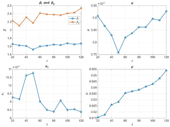
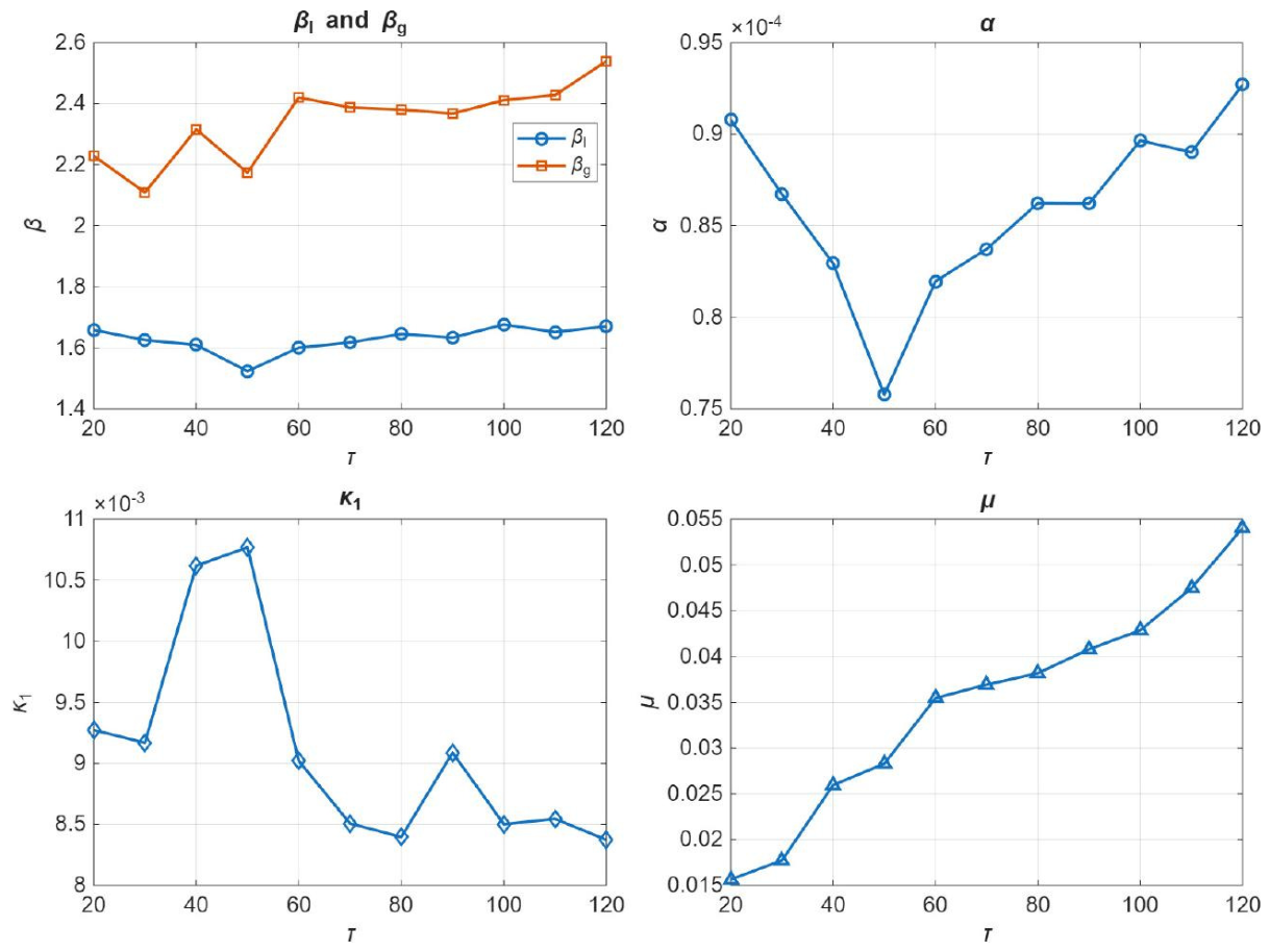
as seen by setting ${\kappa }_1=0$ in Equation (11), whilst $1+{\alpha }_{l,g}/\theta \to {\beta }_{l,g}$. Notice that in Figure 1, both $\beta$ and, consequently, the slopes of the pre-tempered tails show little variation with the number of days of accumulation of returns $\tau$; this is especially true for losses. Also, ${\beta }_l<{\beta }_g$ for any $\tau$, meaning that the power-law parts of losses are slower than those of gains.

Figure 1. Fitted parameters of tempered mJF Skew-t distribution for returns as a function of number of days of accumulation $\tau$.

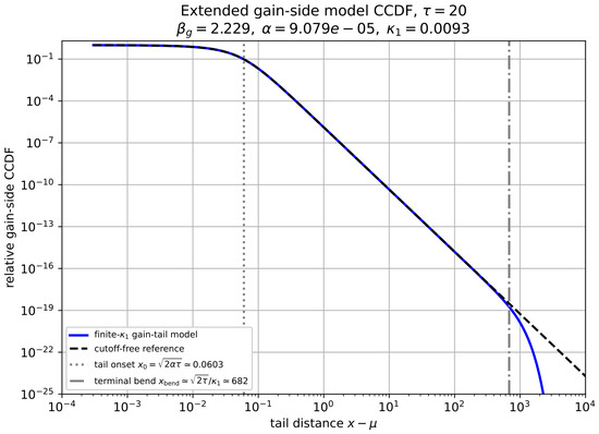
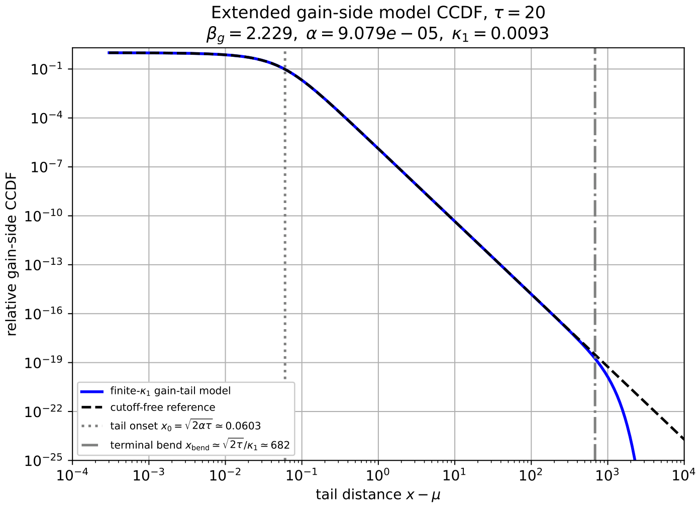
Table 2 shows the parameters derived from Equations (16), (17), (22) and (23) using the fitting parameters from Table 1. Figure 2 illustrates the onset of power-law tails and their eventual bending.

Table 2. Cut-off parameters for stochastic variance ${\kappa }_1^{-2}$ and stochastic volatility ${\kappa }_1^{-1}$; $\theta$ from Equation (22); approximate common tail-distance onset $x_o-\mu$ and common tail-distance bending scale $x_b-\mu$ from Equations (16) and (17); and approximate pre-bending slopes of losses $S_l$ and gains $S_g$ from Equation (23). All values were obtained using the fitting parameters from Table 1 for $\tau =20,30,\dots ,120$ days of accumulation.

$\mathit{\tau }$	${\mathit{\kappa }}_1^{-2}$	${\mathit{\kappa }}_1^{-1}$	$\mathit{\theta }$	${\mathit{x}}_{\mathit{o}}-\mathit{\mu }$	${\mathit{x}}_{\mathit{b}}-\mathit{\mu }$	${\mathit{S}}_{\mathit{l}}$	${\mathit{S}}_{\mathit{g}}$
20	$1.163\times {10}^4$	107.84	$9.623\times {10}^{-5}$	$6.026\times {10}^{-2}$	$6.820\times {10}^2$	−3.316	−4.458
30	$1.189\times {10}^4$	109.06	$1.000\times {10}^{-4}$	$7.213\times {10}^{-2}$	$8.448\times {10}^2$	−3.250	−4.218
40	$8.866\times {10}^3$	94.16	$8.621\times {10}^{-5}$	$8.145\times {10}^{-2}$	$8.422\times {10}^2$	−3.218	−4.630
50	$8.621\times {10}^3$	92.85	$8.929\times {10}^{-5}$	$8.704\times {10}^{-2}$	$9.285\times {10}^2$	−3.046	−4.348
60	$1.229\times {10}^4$	110.86	$8.115\times {10}^{-5}$	$9.917\times {10}^{-2}$	$1.214\times {10}^3$	−3.200	−4.840
70	$1.381\times {10}^4$	117.54	$8.355\times {10}^{-5}$	$1.083\times {10}^{-1}$	$1.391\times {10}^3$	−3.234	−4.774
80	$1.418\times {10}^4$	119.09	$8.517\times {10}^{-5}$	$1.175\times {10}^{-1}$	$1.506\times {10}^3$	−3.290	−4.760
90	$1.211\times {10}^4$	110.05	$8.621\times {10}^{-5}$	$1.246\times {10}^{-1}$	$1.476\times {10}^3$	−3.266	−4.734
100	$1.383\times {10}^4$	117.62	$8.591\times {10}^{-5}$	$1.339\times {10}^{-1}$	$1.663\times {10}^3$	−3.352	−4.822
110	$1.369\times {10}^4$	117.01	$8.563\times {10}^{-5}$	$1.399\times {10}^{-1}$	$1.736\times {10}^3$	−3.302	−4.856
120	$1.426\times {10}^4$	119.42	$8.393\times {10}^{-5}$	$1.492\times {10}^{-1}$	$1.850\times {10}^3$	−3.340	−5.078

Figure 2. Gain-side CCDF from PDF (Equation (19)) with parameters from Table 1 for $\tau =20$. Power-law-like behavior is in effect between approximate common onset $x_o$ from Equation (16) and approximate common bending scale $x_b$ from Equation (17).

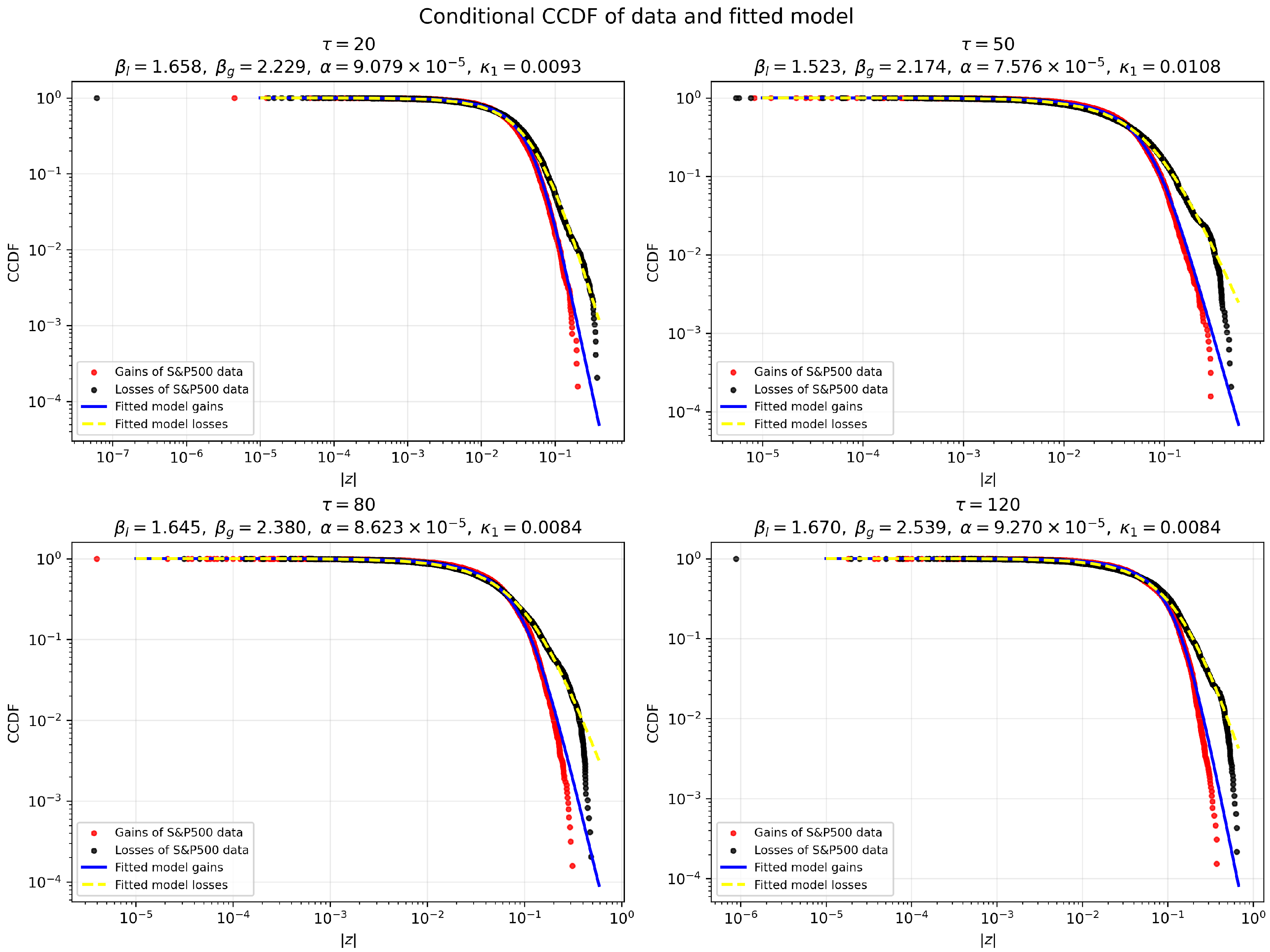
The CCDFs of the fitted distributions with the parameters from Table 1 and Figure 1 were compared with the empirical S&P500 CCDFs in Figure 3. The fits were reasonably good over the observed return range, including the pre-bending power-law regime. However, the model-implied bending scale in Figure 2 lied orders of magnitude beyond the empirical support. Thus, the present data mainly constrain the pre-bending behavior, while the far-tail crossover controlled by ${\kappa }_1$ should be regarded as an asymptotic extrapolation rather than a direct fit to the observed tail termination.

Figure 3. Representative CCDFs for accumulated returns. CCDF of S&P500 gains and losses are plotted vis-a-vis those obtained from fitted distributions (Equation (19)) with parameters from Table 1.

To quantitatively assess the roles of asymmetry and tempering, we compared the proposed tempered mJF distribution with the mJF distribution given by Equation (8) and the symmetric Student t benchmark given by Equation (15). Each model was fitted independently using the maximum likelihood to the same accumulated-return sample. The comparison was performed at $\tau =20$ and $\tau =120$, representing the two endpoints of the investigated accumulation horizon range. Here, AIC denotes the Akaike information criterion, KS denotes the Kolmogorov–Smirnov distance, and AD denotes the Anderson–Darling statistic, which places greater weight on discrepancies in the tails. A larger maximized log-likelihood and smaller AIC, KS, and AD values indicate a better fit, while $\Delta$AIC was measured relative to the lowest AIC at each horizon.

As shown in Table 3, the mJF and tempered mJF models provided nearly indistinguishable fits over the observed support. The tempering parameter produced a small increase in the maximized log-likelihood at both horizons, while the slightly lower AIC of the non-tempered mJF model resulted from its having one fewer parameter. The KS and AD statistics of the two asymmetric models were also nearly identical. By contrast, the symmetric Student t-distribution performed substantially worse according to the log-likelihood, AIC, KS, and AD measures. These results show that the asymmetric mJF structure is important for describing the empirical return distribution, whereas the tempered extension preserves the in-sample fit of the mJF model while providing an asymptotically tempered far-tail form.

Table 3. Maximum-likelihood comparison of the tempered mJF, non-tempered mJF, and Student t-models at the endpoints of the investigated accumulation horizon range. Smaller values for AIC, $\Delta$AIC, KS, and AD indicate a better relative fit.

$\mathit{\tau }$	Model	k	$\log {\mathit{L}}_{\max }$	AIC	$\mathbf{\Delta }$AIC	KS	AD
20	mJF	4	19,955.990	$-39,903.980$	0.000	0.010887	1.960232
20	Tempered mJF	5	19,955.994	$-39,901.987$	1.993	0.010886	1.960295
20	Student-t	3	19,813.514	$-39,621.028$	282.953	0.025923	27.276298
120	mJF	4	9974.285	$-19,940.571$	0.000	0.019219	4.478317
120	Tempered mJF	5	9974.293	$-19,938.585$	1.986	0.019282	4.477508
120	Student-t	3	9770.289	$-19,534.578$	405.993	0.030935	31.017961

3.2. Statistical Parameters

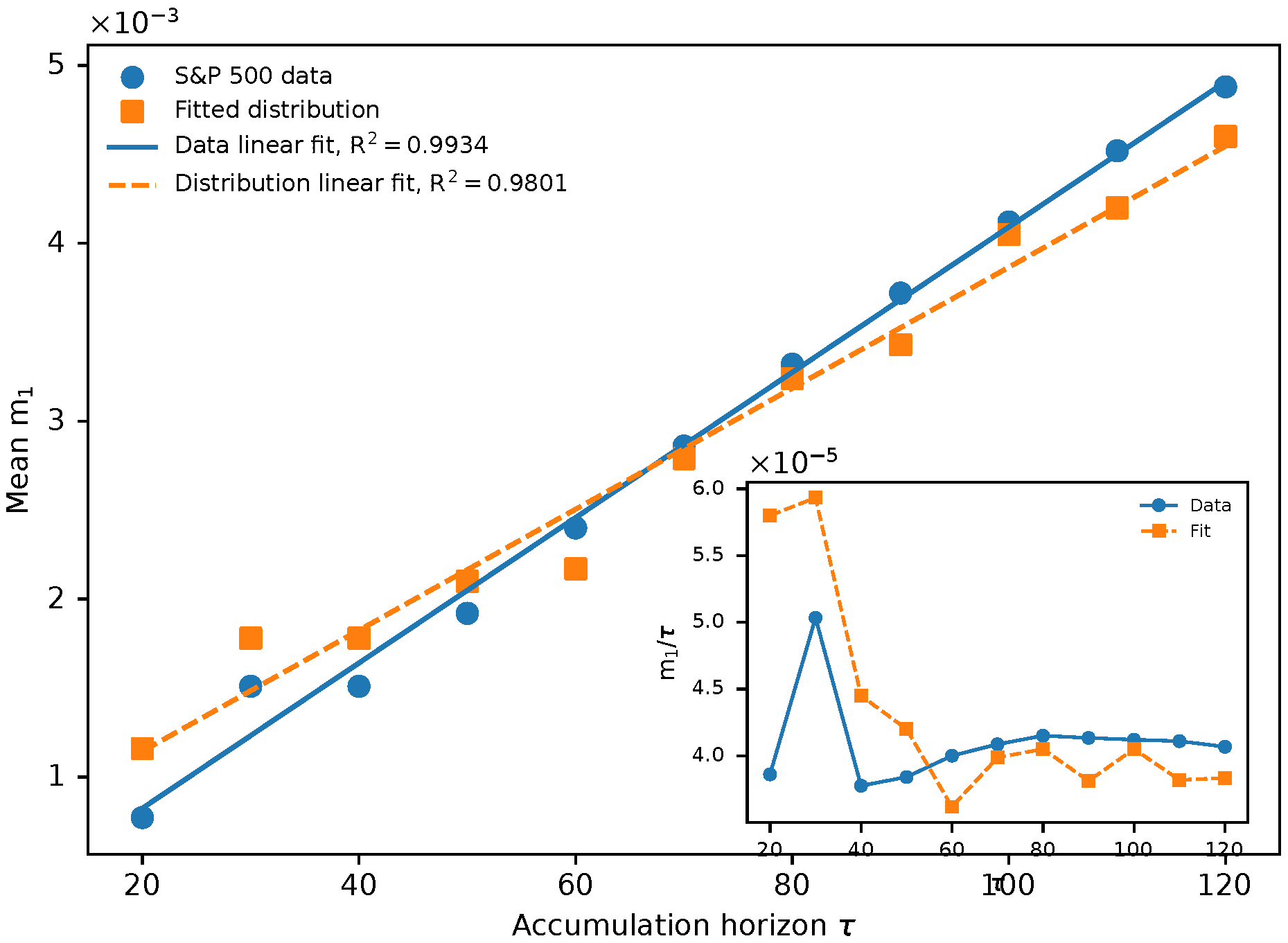
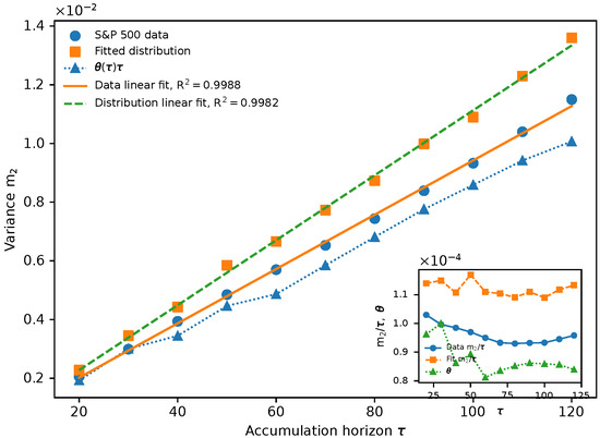
Table 4 contains the values of the mean $m_1$, variance $m_2$, median $\tilde{m}$, and mode $\overline{m}$ of the S&P500 data and those obtained through fitting with the tempered modified Jones–Faddy Skew-t distribution for returns (Equation (19)) over $\tau =20,30,\dots ,120$ days of accumulation of returns. The results contained in Table 4 for the mean $m_1$ and variance $m_2$ are graphically illustrated in Figure 4 and Figure 5, respectively. Linear regressions against the accumulation horizon yielded $R^2=0.9934$ and $0.9801$ for the S&P500 and fitted-distribution means, respectively, and $R^2=0.9988$ and $0.9982$ for the corresponding variances, confirming their near-linear dependence on $\tau$ over the investigated range. The corresponding regression residuals were small relative to the overall variation. We therefore describe the dependence on $\tau$ as near-linear rather than exactly linear. Figure 5 also contains a plot of $\theta \tau$, where $\theta$ is defined by Equation (22). It should be pointed out that for any mean-reverting model of stochastic variance, such as the Cox–Ingersoll–Ross model [23,24,25], the multiplicative model considered here (Equation (5)), and a combined model [26], Equation (6) implies that

$$m_2=⟨\mathrm{d}{x}_t^2⟩=\theta \tau$$

(24)

Table 4. Comparison of mean $m_1$, variance $m_2$, median $\tilde{m}$, and mode $\overline{m}$ between S&P500 data and fitted distribution (Equation (19)).

$\mathit{\tau }$	${\mathit{m}}_1$ Data	${\mathit{m}}_1$ Sim.	${\mathit{m}}_2$ Data	${\mathit{m}}_2$ Sim.	$\tilde{\mathit{m}}$ Data	$\tilde{\mathit{m}}$ Sim.	$\overline{\mathit{m}}$ Data	$\overline{\mathit{m}}$ Sim.
20	0.000772	0.00116	0.00206	0.00228	0.00578	0.00498	0.0124	0.00856
30	0.00151	0.00178	0.00299	0.00345	0.00635	0.00642	0.0193	0.0103
40	0.00151	0.00178	0.00394	0.00443	0.00763	0.00819	0.00953	0.0142
50	0.00192	0.00210	0.00485	0.00585	0.00893	0.00952	0.0118	0.0161
60	0.00240	0.00217	0.00570	0.00666	0.0105	0.0109	0.0129	0.0191
70	0.00286	0.00279	0.00653	0.00773	0.0115	0.0117	0.0212	0.0201
80	0.00332	0.00324	0.00744	0.00873	0.0117	0.0123	0.0203	0.0208
90	0.00372	0.00343	0.00839	0.00999	0.0116	0.0131	0.0155	0.0223
100	0.00412	0.00405	0.00933	0.0109	0.0115	0.0139	0.0116	0.0233
110	0.00452	0.00420	0.0104	0.0123	0.0138	0.0153	0.0137	0.0258
120	0.00488	0.00460	0.0115	0.0136	0.0157	0.0169	0.0206	0.0288

Figure 4. Mean of empirical S&P500 data and of fitted distribution. Insert shows $m_1/\tau$.

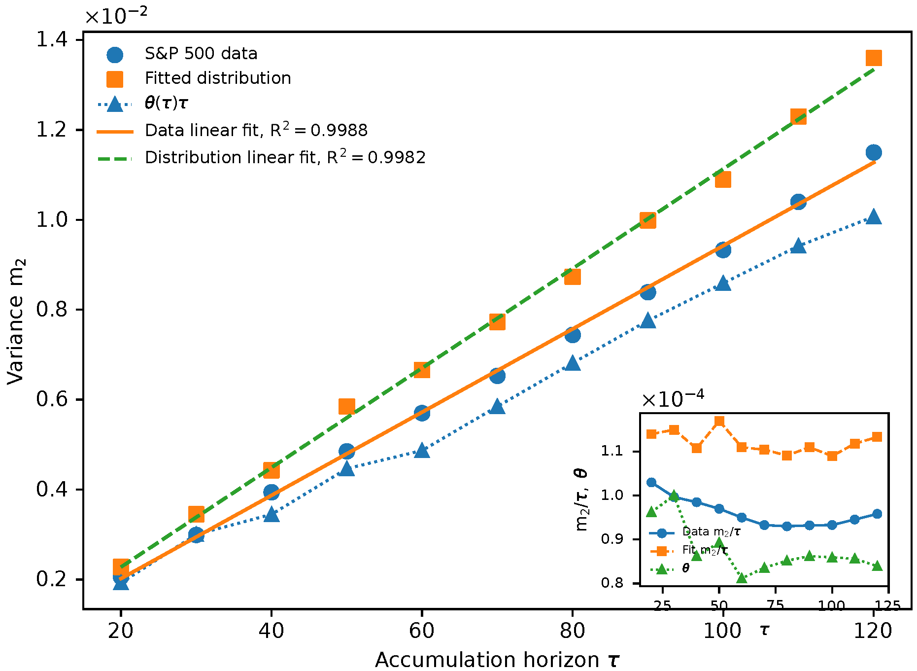
Figure 5. Variance of empirical S&P500 data and of fitted distribution. Also shown is $\theta \tau$ with $\theta$ obtained from Equation (22). Insert shows $m_2/\tau$ and $\theta$.

It is quite remarkable then that even when the symmetry was broken and power-law tails became tempered, the variance $m_2$ still maintained linear dependence on $\tau$, as seen in Figure 5. We dubbed this phenomenon “conservation law” [16]. We emphasize that, per the discussion preceding Equation (22), $\theta$ in Figure 5 no longer directly related to the mean reversion, and it is presented for guidance only. We also note that while some reasoning behind the linear dependence of $m_2$ can be traced back to mean reversion, the linear dependence on $\tau$ of the mean $m_1$ observed in Figure 4 is not presently amenable to a satisfactory explanation.

3.3. Skewness

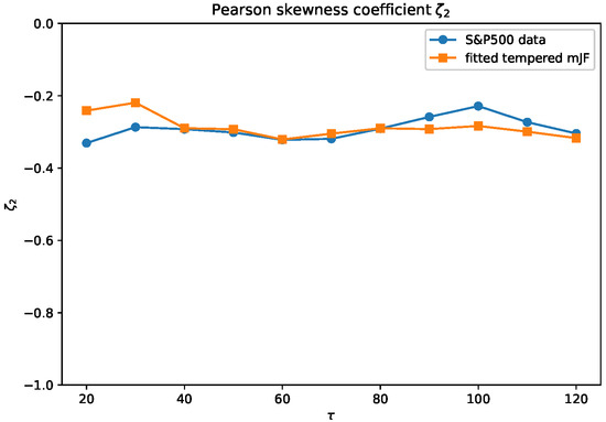
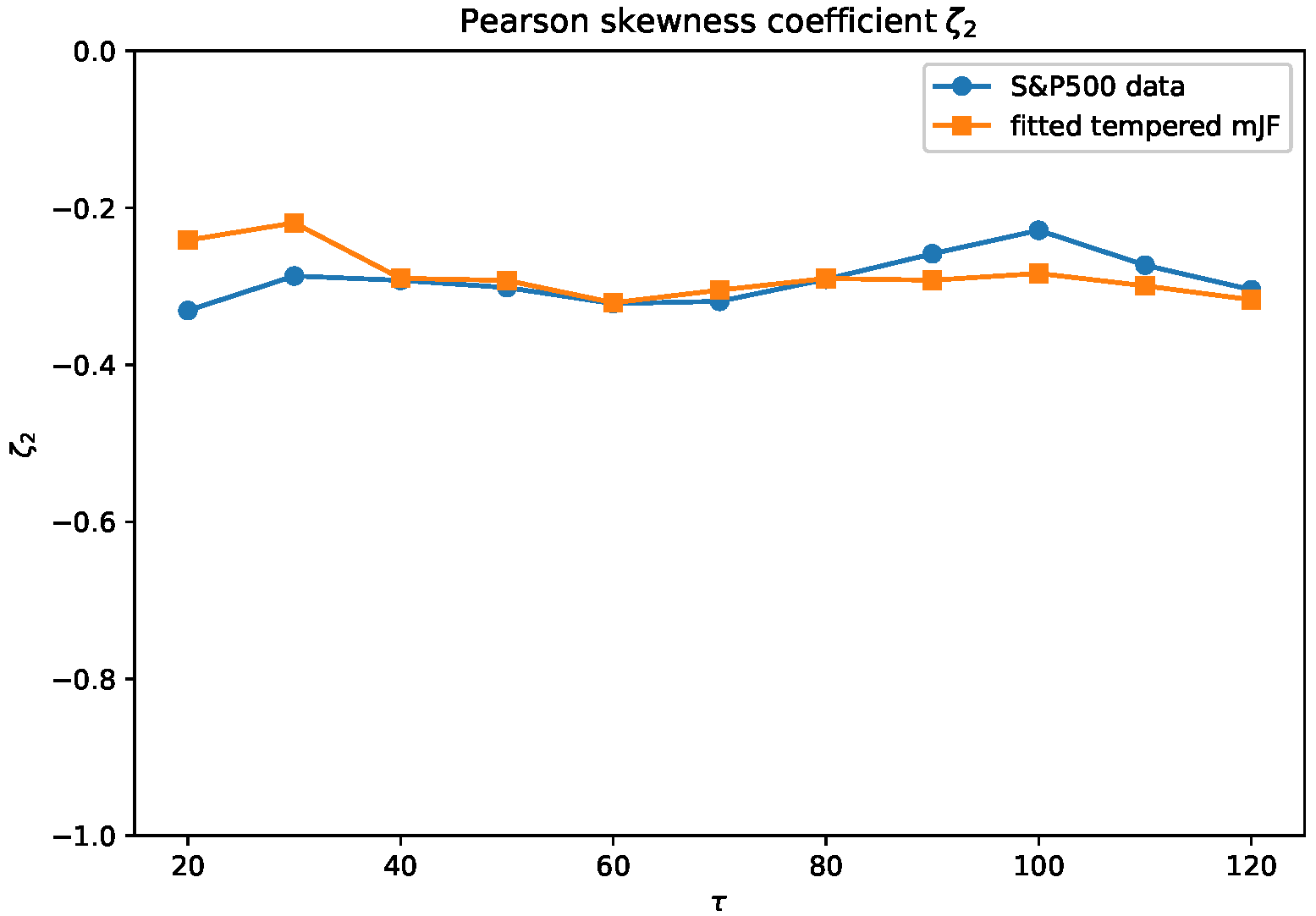
To characterize skewness, we used the first and second Pearson coefficients [27,28], as well as the Fisher–Pearson coefficient [29]:

$${\zeta }_1={\displaystyle \frac{m_1-\overline{m}}{\sqrt{m_2}}},{\zeta }_2={\displaystyle \frac{3(m_1-\tilde{m})}{\sqrt{m_2}}},{\zeta }_{\mathrm{FP}}={\displaystyle \frac{m_3}{m_2^{3/2}}},$$

(25)

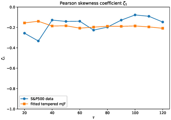
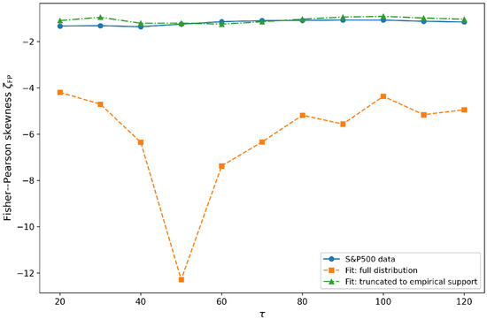
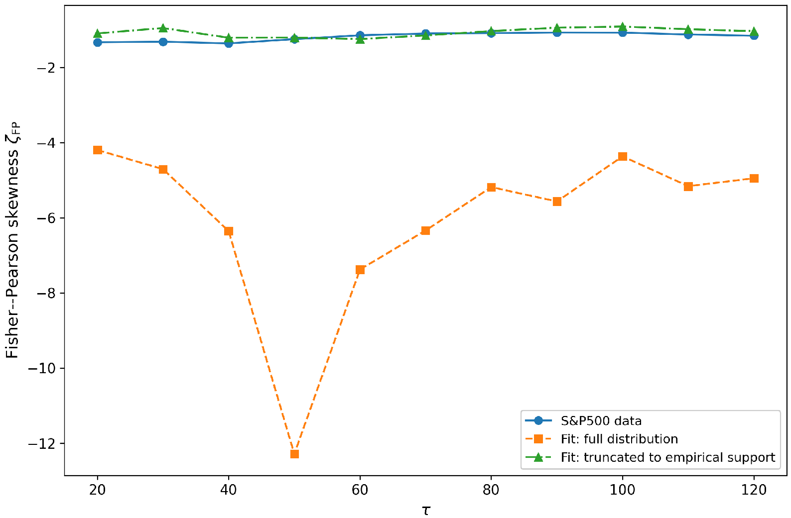
where $m_1$ is the mean, $m_2$ is the variance, $\overline{m}$ is the mode, $\tilde{m}$ is the median, and $m_3=⟨{(x-m_1)}^3⟩$ is the third central moment. In the previous pure power-law setting [16], the Fisher–Pearson coefficient may fail to exist for sufficiently heavy tails. In the present tempered distributions, however, the tails are regularized, and thus the third central moment is finite, and ${\zeta }_{\mathrm{FP}}$ may in principle serve as a meaningful additional diagnostic. Since ${\zeta }_{\mathrm{FP}}$ is particularly sensitive to the far-tail contribution, we report both the Fisher–Pearson skewness of the full fitted distribution and that obtained after truncating and renormalizing the fitted distribution over the empirical support at each accumulation horizon. Table 5 shows ${\zeta }_1$, ${\zeta }_2$, and ${\zeta }_{\mathrm{FP}}$ for the S&P500 data and for the fitted distributions for $\tau =20,30,\dots ,120$ days of accumulated returns, together with the truncated fitted values of ${\zeta }_{\mathrm{FP}}$. A graphical representation of the Pearson coefficients in Table 5 is given in Figure 6, Figure 7 and Figure 8.

Table 5. First and second Pearson skewness coefficients ${\zeta }_1$ and ${\zeta }_2$, respectively, and Fisher–Pearson skewness coefficient ${\zeta }_{\mathrm{FP}}$ for S&P500 data and fitted tempered distributions. The final column reports the fitted Fisher–Pearson skewness after truncation and renormalization over the empirical support.

$\mathit{\tau }$	${\mathit{\zeta }}_1$ Data	${\mathit{\zeta }}_1$ Fit	${\mathit{\zeta }}_2$ Data	${\mathit{\zeta }}_2$ Fit	${\mathit{\zeta }}_{\mathbf{FP}}$ Data	${\mathit{\zeta }}_{\mathbf{FP}}$ Fit, Full	${\mathit{\zeta }}_{\mathbf{FP}}$ Fit, Truncated
20	−0.2565	−0.1551	−0.3310	−0.2400	−1.3316	−4.1973	−1.0938
30	−0.3259	−0.1452	−0.2658	−0.2367	−1.3161	−4.7057	−0.9520
40	−0.1277	−0.1860	−0.2925	−0.2888	−1.3598	−6.3547	−1.2084
50	−0.1412	−0.1831	−0.3017	−0.2910	−1.2468	−12.2880	−1.2056
60	−0.1392	−0.2068	−0.3221	−0.3201	−1.1438	−7.3774	−1.2447
70	−0.2264	−0.1968	−0.3192	−0.3043	−1.0967	−6.3386	−1.1470
80	−0.1968	−0.1881	−0.2911	−0.2897	−1.0875	−5.1850	−1.0324
90	−0.1283	−0.1889	−0.2587	−0.2916	−1.0694	−5.5665	−0.9425
100	−0.0774	−0.1850	−0.2287	−0.2830	−1.0725	−4.3661	−0.9115
110	−0.0906	−0.1950	−0.2732	−0.2998	−1.1226	−5.1608	−0.9842
120	−0.1468	−0.2080	−0.3044	−0.3165	−1.1541	−4.9484	−1.0346

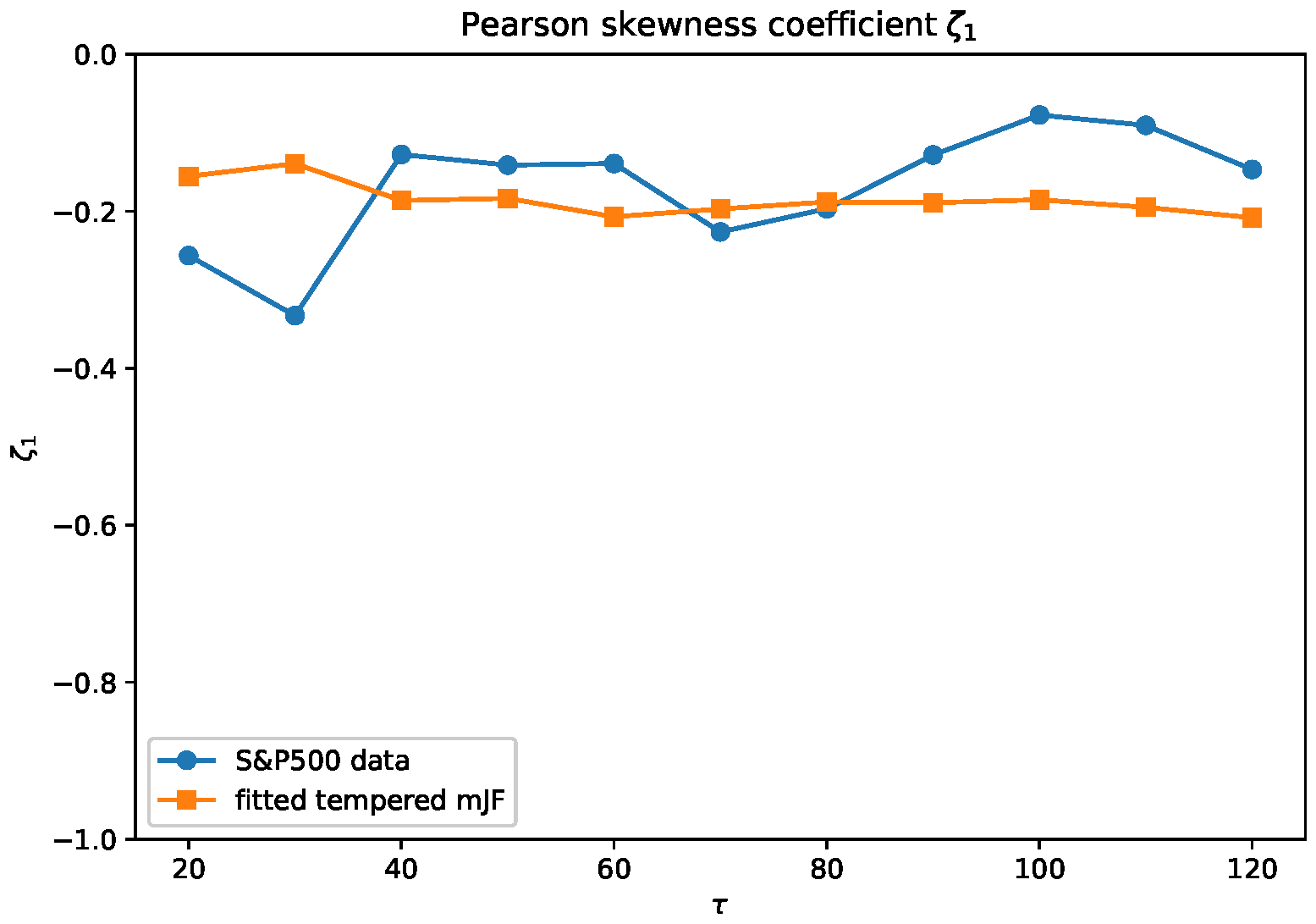
Figure 6. First Pearson skewness coefficients for S&P500 data and fitted distribution as a function of number of days of accumulation of returns.

Figure 7. Second Pearson skewness coefficients for S&P500 data and fitted distribution as a function of number of days of accumulation of returns.

Figure 8. Fisher–Pearson skewness coefficient for the S&P 500 data, the full fitted tempered mJF Skew-t distribution, and the same fitted distribution truncated and renormalized over the empirical support as functions of the accumulation horizon $\tau$.

Clearly, the agreement between the data and the fitted distribution was quite good for ${\zeta }_1$ and ${\zeta }_2$. In addition, these skewness measures depended only weakly on the accumulation horizon, and their negative values were consistent with the heavier tails on the loss side. For the Fisher–Pearson coefficient ${\zeta }_{\mathrm{FP}}$, the full fitted distribution yielded a substantially larger magnitude than the empirical data because the third central moment was highly sensitive to the extrapolated far-tail contribution. To make the comparison with the finite empirical sample more direct, we also computed ${\zeta }_{\mathrm{FP}}$ after truncating and renormalizing the fitted distribution over the empirical support at each horizon. As shown in Figure 8, the truncated fitted values lied much closer to the empirical skewness, indicating that most of the discrepancy in the full-support ${\zeta }_{\mathrm{FP}}$ originated from the far-tail extrapolation rather than from the fit over the observed return range.

4. Scaling

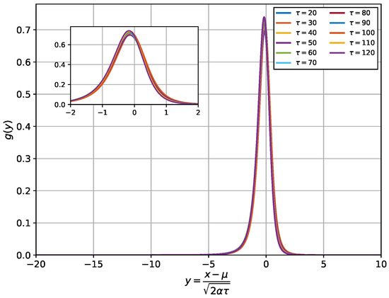
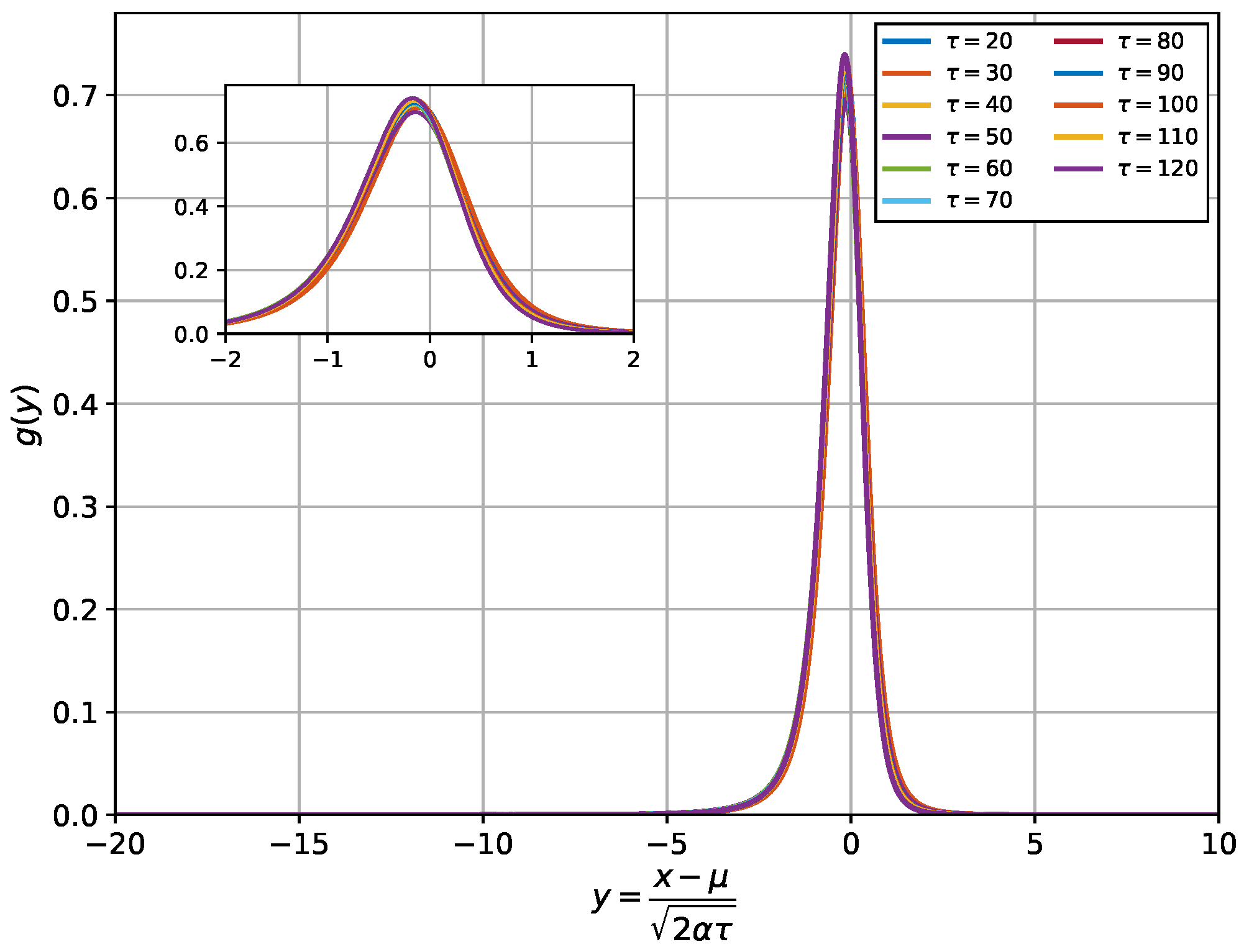
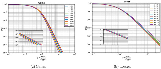
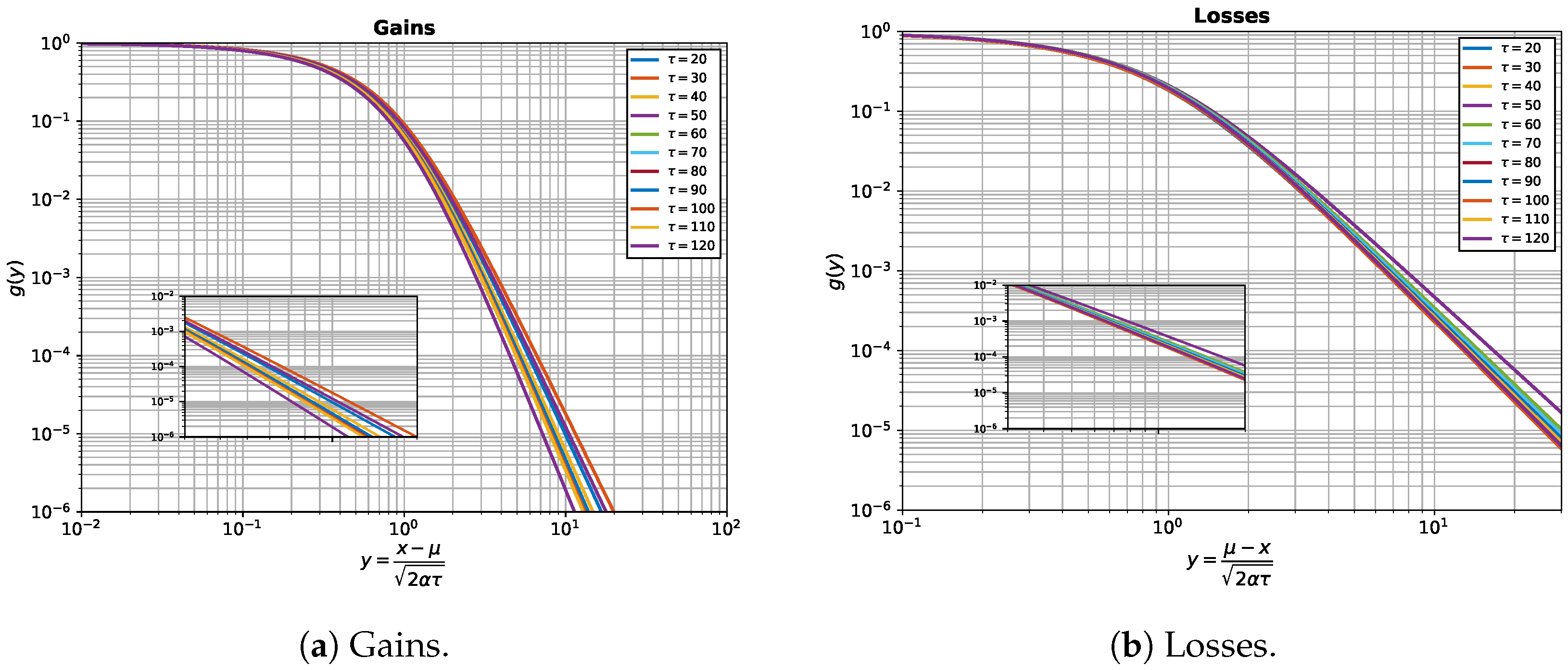
Scaling has been long recognized as a feature of fluctuations in asset prices [9,16,30,31]. The tempered mJF Skew-t distribution for returns fits this mold as well. Indeed, by introducing a new variable

$$y={\displaystyle \frac{x-\mu }{\sqrt{2\alpha \tau }}}$$

and introducing a renormalized tempering parameter

$${\tilde{\kappa }}_1={\kappa }_1{\alpha }^{1/2}$$

then Equation (19) can be rewritten in a rescaled form as follows:

$$\begin{array}{cc}\hfill {\tilde{f}}_{\mathrm{tJF}}\left(y\right)={\displaystyle \frac{1}{\tilde{Z}}}\{& {\displaystyle \frac{3{\tilde{\kappa }}_1^{1+2\overline{\beta }}\Gamma \left(-\frac{1}{2}-\overline{\beta }\right)\Gamma (\overline{\beta }-1)}{4\sqrt{\pi }}}{}_{1}F_1\left({\displaystyle \frac{5}{2}};{\displaystyle \frac{3}{2}}+\overline{\beta };-{\tilde{\kappa }}_1^2\left(y^2+1\right)\right)\hfill \\ \hfill & +\Gamma \left(\overline{\beta }+{\displaystyle \frac{1}{2}}\right){\left(1+{\displaystyle \frac{y}{\sqrt{y^2+1}}}\right)}^{{\beta }_l+{\displaystyle \frac{1}{2}}}{\left[1-{\displaystyle \frac{y}{\sqrt{y^2+1}}}\right]}^{{\beta }_g+{\displaystyle \frac{1}{2}}}\hfill \\ \hfill & \times {}_{1}F_1\left(2-\overline{\beta };{\displaystyle \frac{1}{2}}-\overline{\beta };-{\tilde{\kappa }}_1^2\left(y^2+1\right)\right)\},\overline{\beta }={\displaystyle \frac{{\beta }_l+{\beta }_g}{2}}\hfill \end{array}$$

(26)

thus eliminating the dependence on $\tau$. In this form, the PDF (Equation (26)) can be considered a generic form of the tempered Jones–Faddy Skew-t distribution, now divorced from the specific application to asset returns. In particular, the shape parameters ${\beta }_{l,g}$, previously for “losses” and “gains”, should now be understood as ${\beta }_{l,r}$ for the left and right tails.

It should be pointed out that via a change in variable

$$y={\displaystyle \frac{x}{\sqrt{\overline{\nu }}}}$$

the PDF of the generic Jones–Faddy Skew-t distribution (Equation (4)) can also be written in a rescaled form:

$${\tilde{f}}_{\mathrm{JF}}\left(y\right)={\displaystyle \frac{1}{2^{\overline{\nu }-1}B\left(\frac{{\nu }_l}{2},\frac{{\nu }_r}{2}\right)}}{\left(1+{\displaystyle \frac{y}{\sqrt{y^2+1}}}\right)}^{{\displaystyle \frac{{\nu }_l+1}{2}}}{\left(1-{\displaystyle \frac{y}{\sqrt{y^2+1}}}\right)}^{{\displaystyle \frac{{\nu }_r+1}{2}}},\overline{\nu }={\displaystyle \frac{{\nu }_l+{\nu }_r}{2}}$$

(27)

which elucidates the fact that the tempered Equation (26) is the generalized version of Equation (27) via the tempering parameter ${\tilde{\kappa }}_1$. Obviously, setting ${\beta }_l={\beta }_g=\beta$ in Equation (26) and ${\nu }_l={\nu }_r=\nu$ in Equation (27) would render scaled versions of the tempered Student t-distribution and Equation (1) Student t-distribution, respectively.

Figure 9 and Figure 10 show the PDF (Equation (19)) and the corresponding CCDF for $\tau =20,30,\dots ,120$ as a function of $(x-\mu )/\sqrt{2\alpha \tau }$ using the parameters from Table 1. Clearly, these figures comport well with the idea of scaling embodied in Equation (26).

Figure 9. PDF (19) for $\tau =20,30,\dots ,120$ as a function of $(x-\mu )/\sqrt{2\alpha \tau }$ using parameters from Table 1.

Figure 10. CCDF, corresponding to PDF (Equation (19)), for $\tau =20,30,\dots ,120$ as a function of $(x-\mu )/\sqrt{2\alpha \tau }$ using parameters from Table 1. Inserts show tail areas of CCDF.

5. Discussion

The main result of this work is the introduction of three new distributions. First, we introduced the IGa1 distribution, whose PDF is given by Equations (10) and (11). This distribution is capped at a finite value ${\kappa }_1^{-2}$. However, if $\alpha \ll {\kappa }_1^{-2}$, then IGa1 would exhibit standard IGa power-law tails $\propto v_t^{-\beta -1}$ for $\alpha \ll v_t\ll {\kappa }_1^{-2}$. Second, we introduced a tempered Student t-distribution (Equations (12) and (13)), which is obtained as a product distribution of IGa1 with Gaussian increments of the Wiener process and, as such, exhibits power-law tails with the same exponents as IGa1 between points $x_o$ and $x_b$, estimated in Equations (16) and (17). While this distribution was not capped due to the normal distribution’s infinite support interval, it exhibited significant downward bending after $x_b$, as seen in Figure 2. Lastly, using the Jones–Faddy procedure, we broke the symmetry of the tempered Student t-distribution to obtain a tempered modified Jones–Faddy Skew-t distribution (Equations (19) and (20)), which was characterized by unequal left and right power-law exponents prior to tempering.

We applied a tempered modified Jones–Faddy Skew-t distribution to the analysis of multi-day S&P500 returns for a number of days of accumulation from 20 to 120. Remarkably, the variance in returns (realized variance) showed consistent linear dependence on the number of days of accumulation both for the S&P500 data and for the fitted distributions, as seen in Figure 5. While this is expected for symmetrical distributions according to Equation (6), it is not at all obvious why this should be the case for asymmetrical, tempered distributions, as is the case for empirical data. Furthermore, linear dependence on the number of days of accumulation was also observed for the mean of both the empirical and fitted distributions, as seen in Figure 4. We hope to address the underlying reason for the latter in a future work.

Goodness of fit with the tempered modified Jones–Faddy Skew-t distribution was also confirmed by comparison of the coefficients of skewness in Figure 6 and Figure 7. The asymmetric mJF models substantially outperformed the symmetric Student t-distribution, whereas the tempered and non-tempered mJF models were nearly indistinguishable over the observed support. At the same time, the model-implied bending scale lied orders of magnitude beyond the empirical return range, indicating that the present data mainly constrained the pre-bending power-law regime and only weakly identified the far-tail crossover controlled by ${\kappa }_1$. Consistently, the full-support Fisher–Pearson skewness was strongly affected by the extrapolated far tails, while truncation to the empirical support brought it much closer to the empirical value, as shown in Figure 8. Finally, in Figure 9 and Figure 10, we observe good compliance with the scaling prediction in accordance with Equation (26). While we were specifically addressing the asset returns, Equation (26) can be considered as a generic rescaled tempered Jones–Faddy distribution. The same consideration can be easily applied to rescaled versions of IGa1 and a tempered Student t-distribution.

Aside from the above-mentioned issues left for future work, we also hope to investigate other indices and large-cap individual companies, both domestic and international, to see how prevalent—or not—our findings for S&P500 data are. Additionally, it will be interesting to see whether a tempered Jones–Faddy distribution can be applied to other asset classes, such as housing prices. Finally, we are designing more robust tools for testing the goodness of fit, which is particularly important for distributions with power-law tails.

References

- Fisher, R.A. Applications of `student’s’ distribution. Metron 1925, 5, 90–104. [Google Scholar]
- Martin, B.R. Statistics for Physicists; Academic Press: Cambridge, MA, USA, 1971. [Google Scholar]
- Ahsanullah, M.; Kibria, B.M.G.; Shakil, M. Normal and Student’s t Distributions and Their Applications; Atlantis Press: Dordrecht, The Netherlands, 2014. [Google Scholar]
- Nist Digital Library of Mathematical Functions. Available online: https://dlmf.nist.gov/ (accessed on 13 August 2026).
- Student t-Distribution. Available online: https://reference.wolfram.com/language/ref/StudentTDistribution.html (accessed on 13 August 2026).
- Jones, M.C. Probability and Statistical Models with Applications; Chapman and Hall: London, UK, 2001; Chapter 17; pp. 159–174. [Google Scholar]
- Jones, M.C.; Faddy, M.J. A skew extension of the t-distribution, with applications. J. R. Stat. Soc. B 2003, 65, 159–174. [Google Scholar] [CrossRef] [Scilit]
- Praetz, P.D. The distribution of share price changes. J. Bus. 1972, 45, 49–55. [Google Scholar] [CrossRef] [Scilit]
- Fuentes, M.A.; Gerig, A.; Vicente, J. Universal behavior of extreme price movements in stock markets. PLoS ONE 2009, 4, e8243. [Google Scholar] [CrossRef] [Scilit] [PubMed][Green Version]
- Liu, Z.; Moghaddam, M.D.; Serota, R.A. Distributions of historic market data—Stock returns. Eur. Phys. J. B 2019, 92, 60. [Google Scholar] [CrossRef] [Scilit]
- Nelson, D. Arch models as diffusion approximations. J. Econom. 1990, 45, 7–38. [Google Scholar] [CrossRef] [Scilit]
- Inverse Gamma Distribution. Available online: https://reference.wolfram.com/language/ref/InverseGammaDistribution.html (accessed on 13 August 2026).
- Ma, T.; Serota, R. A model for stock returns and volatility. Phys. A Stat. Mech. Its Appl. 2014, 398, 89–115. [Google Scholar] [CrossRef] [Scilit][Green Version]
- Farahani, H.; Serota, R.A. Asymmetry in distributions of accumulated gains and losses in stock returns. Economies 2025, 13, 176. [Google Scholar] [CrossRef] [Scilit]
- Shao, S.; Ghasemi, A.; Farahani, H.; Serota, R.A. Broken symmetry of stock returns—A modified jones-faddy skew t-distribution. Economies 2026, 14, 84. [Google Scholar] [CrossRef] [Scilit]
- Ghasemi, A.; Shao, S.; Serota, R.A. Broken symmetry, conservation law, and scaling in accumulated stock returns—A modified jones-faddy skew t-distribution perspective. Foundations 2026, 6, 23. [Google Scholar] [CrossRef] [Scilit]
- Ul-Durar, S.; Dimitriadis, K.A.; Arshed, N.; Sisto, M.D.; Harati, H. Distributional and tail-dependent perspectives in economic relationships: A review of quantile regression application. J. Econ. Surv. 2025, 40, 1637–1652. [Google Scholar] [CrossRef] [Scilit]
- Risken, H. The Fokker-Planck Equation; Springer: Berlin/Heidelberg, Germany, 1996. [Google Scholar]
- Jacobs, K. Stochastic Processes for Physicists; Cambridge University Press: Cambridge, UK, 2010. [Google Scholar]
- McDonald, J.B.; Xu, Y.J. A generlazition of the beta distribution with applications. J. Econom. 1996, 66, 133–152. [Google Scholar] [CrossRef] [Scilit]
- Rohatgi, V.K. An Introduction to Probability Theory and Mathematical Statistics, 1st ed.; Wiley Series in Probability and Statistics; Wiley: Hoboken, NJ, USA, 1976. [Google Scholar]
- Grimmett, G.; Stirzaker, D. Probability and Random Processes, 4th ed.; Oxford University Press: Oxford, UK, 2020. [Google Scholar]
- Cox, J.; Ingersoll, J.; Ross, S. A theory of the term structure of interest rates. Econometrica 1985, 3, 385–408. [Google Scholar] [CrossRef] [Scilit]
- Heston, S.L. A closed-form solution for options with stochastic volatility with applications to bond and currency options. Rev. Financ. Stud. 1993, 6, 327–343. [Google Scholar] [CrossRef] [Scilit]
- Drǎgulescu, A.A.; Yakovenko, V.M. Probability distribution of returns in the heston model with stochastic volatility. Quant. Financ. 2002, 2, 443–453. [Google Scholar] [CrossRef] [Scilit]
- Moghaddam, M.D.; Serota, R.A. Combined mutiplicative-heston model for stochastic volatility. Phys. A Stat. Mech. Its Appl. 2021, 561, 125263. [Google Scholar] [CrossRef] [Scilit]
- Pearson, K. Contributions to the mathematical theory of evolution. Philos. Trans. R. Soc. Lond. A 1894, 185, 71–110. [Google Scholar] [CrossRef] [Scilit]
- Pearson, K. Contributions to the mathematical theory of evolution. ii. skew variation in homogeneous material. Philos. Trans. R. Soc. Lond. A 1895, 186, 343–414. [Google Scholar] [CrossRef] [Scilit]
- Fisher, R.A. The moments of the distribution for normal samples of measures of departures from normality. Proc. R. Soc. Lond. A 1930, 130, 16–28. [Google Scholar] [CrossRef] [Scilit]
- Mantegna, R.N.; Stanley, H.E. Scaling behaviour in the dynamics of an economic index. Nature 1995, 376, 46–49. [Google Scholar] [CrossRef] [Scilit]
- Gopikrishnan, P.; Plerou, V.; Amaral, L.A.N.; Meyer, M.; Stanley, H.E. Scaling of the distribution of fluctuations of financial market indices. Phys. Rev. E 1999, 60, 5305–5316. [Google Scholar] [CrossRef] [Scilit] [PubMed]
Disclaimer/Publisher’s Note: The statements, opinions and data contained in all publications are solely those of the individual author(s) and contributor(s) and not of MDPI and/or the editor(s). MDPI and/or the editor(s) disclaim responsibility for any injury to people or property resulting from any ideas, methods, instructions or products referred to in the content. |
© 2026 by the authors. Licensee MDPI, Basel, Switzerland. This article is an open access article distributed under the terms and conditions of the Creative Commons Attribution (CC BY) license.