On the Axiom of the Second Law of Thermodynamics and the Modelling of Flexoelectricity

Abstract

The present paper addresses models of non-local materials and, in particular, flexoelectric materials as dielectrics with higher-order gradients. While the literature develops the subject through variational formulations, here the modelling is developed within a thermodynamic framework with a general form of the Clausius–Duhem inequality, where the extra-entropy flux and the entropy production are given by constitutive functions. Furthermore, the polar character of the material, associated with flexoelectricity, is modelled by a body couple and no use is made of hyper-stresses. As a result of the thermodynamic analysis, it follows that the symmetric part of the stress and the electric polarization are given by a variational derivative of the electric enthalpy along with the dissipative parts that involve the selected function of entropy production. The skewed part of the stress is shown to be free from thermodynamic restrictions and is simply required to counterbalance the body couple.

1. Introduction

This paper addresses the formulation and application of the second law of thermodynamics in continuum physics. Since the publication of the paper by Coleman and Noll [1], the second law provides a procedure for the selection of physically admissible models through appropriate constitutive equations. Formally, the second law is based on the principle of an increase in entropy, and in mathematical terms, the increase is expressed by saying that the time derivative, $\dot{\eta }$, of the specific entropy density, $\eta$, deprived of the contribution, $(\nabla ·\mathbf{j})/\rho$, of the entropy flux, $\mathbf{j}$, and that of the entropy supply, s, equals the positive entropy production density, $\gamma$, viz.

$$\dot{\eta }+(\nabla ·\mathbf{j})/\rho -s=\gamma \ge 0,$$

(1)

where $\rho$ is the mass density. The material selection of the second law is based on the postulate that only models that satisfy inequality (1) are physically admissible. In this paper, formal details on the application of (1) are developed in connection with flexoelectricity. Here, we underline two general aspects related to (1).

In [1], Coleman and Noll assumed that the entropy flux, $\mathbf{j}$, equals the heat flux, $\mathbf{q}$, divided by the absolute temperature, $\theta$. Next, Müller [2] generalized the postulate by letting $\mathbf{j}$ be given by a constitutive equation to be determined subject to (1). Once the balance of energy is considered through the entropy supply, s, the entropy inequality (1) can be written in the form

$$f+\theta \nabla ·\mathbf{k}=\rho \theta \gamma \ge 0,$$

(2)

where $\mathbf{k}=\mathbf{j}-\mathbf{q}/\theta$, and f denotes the chosen variables and their time derivatives. Given f, the inequality (2) holds for appropriate expressions of $\mathbf{k}$ and $\gamma$ [3]. Indeed, non-zero expressions of $\mathbf{k}$ occur when non-local models are considered, where constitutive functions depend on gradients of suitable order [4]. This is the physical case of flexoelectricity, as shown in this paper.

Usually, Equation (1) is viewed as the definition of $\gamma$ in that equality is viewed as an identity. Now, rate-type equations that describe hysteretic properties need to distinguish the response depending on the signs of suitable derivatives. This is the case for, e.g., hysteresis in plasticity and ferromagnetism [5,6]. More recently, a continuum model has been established for SMAs in terms of the temperature, $\theta$, the (uniaxial) stress, $\sigma$, and the mass fraction, $\xi$. For definiteness, at constant stress, the expression of (1) reads

$${\partial }_{\xi }\varphi (-k\dot{\theta }-\dot{\xi })=\theta \gamma ,$$

where $\varphi$ is the free energy. A realistic behaviour for SMAs is obtained by letting

$$\theta \gamma =\mu |{\partial }_{\xi }\varphi \left|\right|\dot{\theta }|,\mu >0,$$

whence

$$k\dot{\theta }+\dot{\xi }=-\mu \mathrm{sgn}({\partial }_{\xi }\varphi )\left|\dot{\theta }\right|.$$

(3)

Equation (3) shows that the evolution of $\xi$ depends on $\mathrm{sgn}\dot{\theta }$, as is customary in hysteresis induced by temperature, but also on $\mathrm{sgn}({\partial }_{\xi }\varphi )$, namely on the half space on the side of ${\partial }_{\xi }\varphi =0$. Accordingly, $\gamma \ge 0$, as is required by the increase in entropy (inequality in (1)); meanwhile,

$$\theta \gamma ={\partial }_{\xi }\varphi (-k\dot{\theta }-\dot{\xi })$$

though $\theta \gamma$ and ${\partial }_{\xi }\varphi (-k\dot{\theta }-\dot{\xi })$ are not identically equal.

As a remarkable application of the second law, this paper investigates the modelling of flexoelectricity. The flexoelectric effect is the response of electric polarization to a strain gradient. While piezoelectricity denotes the generation of an electric polarization by a mechanical strain, flexoelectricity represents a further effect on polarization due to a strain gradient. From a physical viewpoint, piezoelectricity does not occur in dielectric materials with inversion-centred symmetry; the strain gradient is more effective in that the gradient can break the inversion symmetry and then generate polarization, even in non-piezoelectric materials. Furthermore, the remarkable interest in flexoelectricity is due also to the prevalence of micro- and nano-scale materials, where large strain gradients more frequently occur.

Modelling with strain gradients poses interesting mathematical problems, in that the stress tensor need not be symmetric and, according to the literature, difficulties arise in terms of the stress power. Also appealing to the principle of virtual work [7,8], balance equations are often established by considering the higher-order counterparts of stress tensors and the electric field. Otherwise, the procedure is based on a variational approach through a functional with an appropriate energy function and the application of thermodynamic conjunctions for completing balance equations (see, e.g., [9,10]). To account for non-symmetric stress, micropolar schemes provide a recourse (see [11] and the references therein).

A systematic thermodynamic theory is in order for flexoelectric materials. This means that, upon a clear set of balance equations, the constitutive properties have to be derived through the restrictions placed by the second law of thermodynamics. This problem is of interest mathematically because, as is the case for non-local models [4], higher-order derivatives need to be framed within a thermodynamic setting. The purpose of this paper is to develop a thermodynamic approach to polar materials by a detailed derivation of the constitutive functions of polar deformable solids subjected to an electric field.

The polar character of flexoelectric materials calls for a preliminary revisit of balance equations. The presence of a body couple makes the stress tensor non-symmetric (see Appendix A). Consequently, an inspection of the balance of energy is given in Section 2 and a restatement of the second law of thermodynamics is provided (Section 3), along with the corresponding restrictions for a polar body (Section 4). Proceeding along the lines of recent approaches to the modelling of non-local and/or hysteretic materials, it emerges that the entropy production, $\gamma$, must also be given by a constitutive function subject to the second law inequality (1). Next, the restrictions placed by the second law inequality are derived for the dissipative parts of the stress tensor and the electric polarization (Section 5).

2. Notation and Balance of Energy

Let $\Omega$ be the time-dependent region occupied by the body. The position of a point in $\Omega$ is denoted by the vector $\mathbf{x}$, relative to a chosen origin, O, as a function of the time, t, while the position in a reference configuration, $\mathrm{R}$, is denoted by $\mathbf{X}$. So, $\mathbf{x}=\mathbf{x}(\mathbf{X},t)$, as $t\in \mathbb{R}$ describes the motion of $\mathbf{X}$. For definiteness, the components of the vectors are considered relative to a right-handed orthonormal triplet, ${\mathbf{e}}_1,{\mathbf{e}}_2,{\mathbf{e}}_3$. We denote by ∇ and $\nabla R$ the gradient operators with respect to $\mathbf{x}$ and $\mathbf{X}$. The gradient $\nabla R\mathbf{x}$ is called the deformation gradient and denoted by $\mathbf{F}$; in the components, $F_{iK}={\partial }_{X_K}{x}_i$. The difference $\mathbf{u}=\mathbf{x}-\mathbf{X}$ is called the displacement, and then $\mathbf{H}=\nabla R\mathbf{u}$, viz. $H_{iK}={\partial }_{X_K}{u}_i$, is the displacement gradient and $\mathbf{F}=\mathbf{1}+\mathbf{H}$, with $\mathbf{1}$ being the identity tensor. The tensor $\mathbf{C}={\mathbf{F}}^T\mathbf{F}$ is the symmetric Cauchy–Green strain tensor. If, for any entry, $H_{iK}$, it is $|H_{iK}|\ll 1$, then

$$H_{iK}={\partial }_{X_K}{u}_i={\partial }_{x_j}{u}_i{F}_{jK}\simeq {\partial }_{x_j}{u}_i{\delta }_{jK}={\partial }_{x_K}{u}_i.$$

Hence, if $|H_{iK}|\ll 1$, then the Green–Lagrange strain $\frac{1}{2}(\mathbf{C}-\mathbf{1})$ may be approximated by

$$\frac{1}{2}(\mathbf{C}-\mathbf{1})=\frac{1}{2}({\mathbf{H}}^T+\mathbf{H}+{\mathbf{H}}^T\mathbf{H})\simeq \mathrm{sym}\nabla \mathbf{u}=:\mathit{ϵ}.$$

The tensor $\mathit{ϵ}$ is called infinitesimal strain. A superposed dot denotes the material (or Lagrangian) time derivative. For any function, $\phi (\mathbf{x},t)$, it is

$$\dot{\phi }={\partial }_t\phi +(\mathbf{v}·\nabla )\phi ,$$

where $\mathbf{v}=\dot{\mathbf{x}}$ is the velocity. The tensor $\mathbf{L}$ denotes the velocity gradient, $L_{ij}=v_{i,j}$, and $\mathbf{D}=\mathrm{sym}\mathbf{L}$, with $\mathrm{sym}$ denoting the symmetric part, $\mathrm{sym}\mathbf{L}=\frac{1}{2}(\mathbf{L}+{\mathbf{L}}^T)$.

The balance of linear and angular momentum is summarized in the Appendix A. Here, we revisit the balance of energy, as it is essential for second law inequality.

The balance of energy involves the energy density, $\rho (\frac{1}{2}{\mathbf{v}}^2+\frac{1}{2}\mathit{\omega }·\mathbf{I}(\mathit{\omega })+\epsilon )$, the body power, $\rho (\mathbf{b}·\mathbf{v}+w+r)$, and the surface power density, $\mathbf{t}·\mathbf{v}+h$, where the energy density, $\epsilon$, and the powers, r and h, are terms of non-mechanical character. The term w is an internal power and, dealing with polar dielectrics, w consists of the electrical power, $w=\mathbf{E}·\dot{\mathit{\pi }}$, and the mechanical power, $\mathbf{c}·\mathit{\omega }$. Hence, the balance is assumed in the form

$$\begin{array}{c}\hfill {\displaystyle \frac{d}{dt}}{\int }_{\mathcal{P}}\rho (\frac{1}{2}{\mathbf{v}}^2+\frac{1}{2}\mathit{\omega }·\mathbf{I}(\mathbf{\omega })+\epsilon )dv={\int }_{\mathcal{P}}[\rho (\mathbf{b}·\mathbf{v}+\mathbf{E}·\dot{\mathit{\pi }}+r)+\mathbf{c}·\mathit{\omega }]dv\\ \hfill +{\int }_{\partial \mathcal{P}}(\mathbf{t}·\mathbf{v}+h)da.\end{array}$$

Notice that

$$\left[\mathbf{I}(\mathit{\omega })\right]\dot{}=\mathbf{I}(\dot{\mathit{\omega }})+\mathit{\omega }\times \mathbf{I}(\mathit{\omega }),$$

and then, using the symmetry of $\mathbf{I}$, we have

$$[\mathit{\omega }·\mathbf{I}(\mathit{\omega })]\dot{}=\dot{\mathit{\omega }}·\mathbf{I}(\mathit{\omega })+\mathit{\omega }·\mathbf{I}(\dot{\mathit{\omega }})=2\mathit{\omega }·\mathbf{I}(\dot{\mathit{\omega }}).$$

Accordingly, in light of Equations (A2) and (A4), we obtain

$${\int }_{\mathcal{P}}\rho \dot{\epsilon }-\rho r-\rho \mathbf{E}·\dot{\mathit{\pi }}-\mathbf{T}·\mathbf{L}+\mathbf{{\rm Y}}·\mathit{\omega })dv={\int }_{\partial \mathcal{P}}hda.$$

As with the balance of forces and the corresponding Cauchy’s theorem about the force density per unit area, $\mathbf{t}$, we observe that equality among volume and surface integrals hold only if the surface density has a particular form. Indeed, Cauchy’s theorem for the dependence of $\mathbf{t}$ on the normal, $\mathbf{n}$, to the surface leads to the relation [12,13]

$$h(\mathbf{n})={\sum }_{i=1}^{3}h({\mathbf{e}}_i){\mathbf{e}}_i·\mathbf{n}.$$

Letting

$$\mathbf{q}=-{\sum }_{i=1}^{3}h({\mathbf{e}}_i){\mathbf{e}}_i$$

we have

$$h(\mathbf{n})=-\mathbf{q}·\mathbf{n}.$$

Hence, using the divergence theorem, we find the balance of energy, $\epsilon$, in the form

$$\rho \dot{\epsilon }=\mathbf{T}·\mathbf{L}-\mathbf{{\rm Y}}·\mathit{\omega }+\rho \mathbf{E}·\dot{\mathit{\pi }}-\nabla ·\mathbf{q}+\rho r.$$

(4)

Accordingly, $\mathbf{q}$ is identified with the heat flux vector while r is the heat supply.

Split the stress tensor, $\mathbf{T}$, in the symmetric and skewed parts,

$$\mathbf{T}={\mathbf{T}}^{sym}+{\mathbf{T}}^{skw}.$$

Since $\mathbf{L}=\mathbf{D}+\mathbf{W}$, we have

$$\mathbf{T}·\mathbf{L}=\mathbf{T}·\mathbf{D}+\mathbf{T}·\mathbf{W}.$$

Hence, letting

$$W_{ij}=-{ϵ}_{ijq}{w}_q$$

we find

$${\mathbf{T}}^{skw}·\mathbf{W}=T_{ij}^{skw}{W}_{ij}=\mathbf{{\rm Y}}·\mathbf{w},\mathbf{w}=\frac{1}{2}\nabla \times \mathbf{v}$$

with the axial vector, $\mathbf{w}$, being viewed as the angular velocity of the macroscopic motion. Hence, the balance of energy (4) can be given the form

$$\rho \dot{\epsilon }=\mathbf{T}·\mathbf{D}+\mathbf{{\rm Y}}·(\mathbf{w}-\mathit{\omega })+\rho \mathbf{E}·\dot{\mathit{\pi }}-\nabla ·\mathbf{q}+\rho r,$$

(5)

with $\mathbf{w}-\mathit{\omega }$ as the difference between the angular velocity of the macroscopic continuum and that of the micropolar continuum.

A polar dielectric may be modelled by ignoring the internal degree of freedom of the micropolar structure. In that case, $\mathbf{l}=\mathbf{0}$, and the mechanical power of the body couple is $\mathbf{c}·\mathbf{w}$, so we ascribe to the local angular velocity, $\mathit{\omega }$, the value $\mathbf{w}$. Hence, by (A5), we have $\mathbf{c}·\mathbf{w}=-\mathbf{{\rm Y}}·\mathbf{w}$, and the mechanical power takes the form

$$\mathbf{T}·\mathbf{L}+\mathbf{c}·\mathbf{w}={\mathbf{T}}^{sym}·\mathbf{D}.$$

Consequently, the balance of energy reads

$$\rho \dot{\epsilon }={\mathbf{T}}^{sym}·\mathbf{D}+\rho \mathbf{E}·\dot{\mathit{\pi }}-\nabla ·\mathbf{q}+\rho r,$$

(6)

as it follows from (5) with $\mathit{\omega }=\mathbf{w}$.

One may ask whether the simplification of the mechanical power in Equation (6) is self-consistent from a physical standpoint in that we know that, in polar media, the stress tensor, $\mathbf{T}$, need not be symmetric. Indeed, as derived in the Appendix A, the skewed part of $\mathbf{T}$ enters the evolution equation of the micropolar angular momentum, $\mathbf{l}$ (see Equation (A4)). If $\mathbf{l}=\mathbf{0}$, then the stress vector, $\mathbf{Y}$, balances the body couple, $\mathbf{c}$. Consequently, the balance of energy (5) involves $\mathbf{Y}$ through the power $\mathbf{Y}·(\mathbf{w}-\mathit{\omega })$. Usually, this term is not considered in the literature. As shown above, this amounts to disregarding the micropolar angular momentum, $\mathbf{l}$, and to letting $\mathit{\omega }=\mathbf{w}$, so that the micropolar angular velocity is taken to be equal to the macroscopic angular velocity, $\mathbf{w}$. The present derivation may be a justification of the use of the balance relation (6).

3. Second Law for Continuous Bodies

From the thermodynamics of homogeneous bodies (see, e.g., [14], ch. 8), we take the existence of the entropy, S, and the absolute temperature, $\theta \ge 0$, so that, if Q is the heat exchanged reversibly at temperature $\theta$, then the change $\Delta S$ of S is

$$\Delta S={\displaystyle \frac{Q}{\theta }}.$$

Furthermore, the entropy of an isolated body cannot decrease in time (principle of increase in entropy).

We now look for an appropriate statement about entropy in continuum physics. We start with the balance of entropy based on the view that the time derivative of a volume integral of a field is given by a volume integral and a surface integral of suitable fields. Let $\eta$ be the entropy density per unit mass. Then, for any subregion, $\mathcal{P}$, convecting with the body, we assume

$${\displaystyle \frac{d}{dt}}{\int }_{\mathcal{P}}\rho \eta dv={\int }_{\mathcal{P}}\rho sdv+{\int }_{\partial \mathcal{P}}\phi da,$$

(7)

and then $\rho s$ is the entropy supply, per unit volume, while $\phi$ is the entropy provided per unit area. By using Reynolds’ transport theorem, we can write

$${\displaystyle \frac{d}{dt}}{\int }_{\mathcal{P}}\rho \eta dv={\int }_{\mathcal{P}}\rho \dot{\eta }dv.$$

Hence, Equation (7) may be written in the form

$${\int }_{\mathcal{P}}\rho (\dot{\eta }-s)dv={\int }_{\partial \mathcal{P}}\phi da.$$

(8)

As with the balance of forces and the corresponding Cauchy’s theorem about the force density per unit area $\mathbf{t}$, we observe that equality among volume and surface integrals hold only if the surface density has a particular form. Indeed, Cauchy’s theorem for the dependence of $\mathbf{t}$ on the normal, $\mathbf{n}$, to the surface leads to the relation [12,13]

$$\mathbf{t}(\mathbf{n})={\sum }_{i=1}^3\mathbf{t}({\mathbf{e}}_i)(\mathbf{n}·{\mathbf{e}}_i).$$

In the same way, for field $\phi$, we have

$$\phi (\mathbf{n})={\sum }_{i=1}^3\phi ({\mathbf{e}}_i){\mathbf{e}}_i·\mathbf{n}.$$

Letting

$$j_i=-\phi ({\mathbf{e}}_i)\mathrm{or}\mathbf{j}=-{\sum }_{i=1}^3\phi ({\mathbf{e}}_i){\mathbf{e}}_i$$

we have

$$\phi (\mathbf{n})=-\mathbf{j}·\mathbf{n}.$$

(9)

By the divergence theorem

$${\int }_{\partial \mathcal{P}}\mathbf{j}·\mathbf{n}da={\int }_{\mathcal{P}}\nabla ·\mathbf{j}dv.$$

Hence, Equation (8) becomes

$${\int }_{\mathcal{P}}(\rho \dot{\eta }+\nabla ·\mathbf{j}-\rho s)dv=0.$$

Since $\mathcal{P}$ is an arbitrary subregion of the body, and assuming the continuity of the integrand, it follows that

$$\rho \dot{\eta }+\nabla ·\mathbf{j}-\rho s=0.$$

For $\mathbf{j}$ and s, we follow the classical content of the contribution $Q/\theta$ to the entropy and let

$$\mathbf{j}={\displaystyle \frac{\mathbf{q}}{\theta }}+\mathbf{k},s={\displaystyle \frac{r}{\theta }}+\gamma ,$$

with $\mathbf{q}/\theta$ and $r/\theta$ being the local versions of $Q/\theta$, while $\mathbf{k}$ and $\gamma$ are possible additional terms. Consistent with the definition, $\mathbf{k}$ is called the extra-entropy flux. Hence, we have

$$\rho \dot{\eta }+\nabla ·({\displaystyle \frac{\mathbf{q}}{\theta }}+\mathbf{k})-\rho {\displaystyle \frac{r}{\theta }}=\rho \gamma .$$

(10)

Accordingly, $\gamma$ is the rate of entropy when no interaction with the environment occurs. The principle of increase in entropy then implies that

$$\gamma \ge 0.$$

(11)

A thermodynamic process is the set of functions on $\Omega \times \mathbb{R}$ that satisfy the balance Equations (4), (10), (A1) and (A2). The physical nature of a thermodynamic process is specified by the non-negative property of $\gamma$, which represents the principle of increase in entropy. This aspect is made formal by generalizing a famous axiom by Coleman and Noll [1]:

Postulate 1. 

The inequality (11) holds for all admissible thermodynamic processes.

Consequently, the requirement (11) becomes

$$\rho \dot{\eta }+\nabla ·({\displaystyle \frac{\mathbf{q}}{\theta }}+\mathbf{k})-\rho {\displaystyle \frac{r}{\theta }}=\rho \gamma \ge 0,$$

(12)

this condition being called the Clausius–Duhem (CD) inequality. The energy supply $r(\mathbf{x},t)$ is an arbitrary function. Using the arbitrariness of r, we have to be consistent and let r in (12) be the same as that used in (4). Hence, we replace r from (4) to obtain (12) in the form

$$\rho \theta \dot{\eta }-(\rho \dot{\epsilon }-\lambda )=\rho \theta \gamma +{\displaystyle \frac{1}{\theta }}\mathbf{q}·\nabla \theta =:\delta ,$$

where $\lambda$ is the pertinent power: here, $\lambda ={\mathbf{T}}^{sym}·\mathbf{D}+\mathbf{{\rm Y}}·(\mathbf{w}-\mathit{\omega })+\rho \mathbf{E}·\dot{\mathit{\pi }}$. This requirement

$$\delta \ge 0$$

is referred to as Planck inequality and is equivalent to the CD inequality when $\nabla \theta =\mathbf{0}$ and $\mathbf{k}=\mathbf{0}$ (see [15], Lect. 2). Letting $\epsilon =\psi +\theta \eta +\mathbf{E}·\mathit{\pi }$, we obtain the CD inequality in the form

$$-\rho (\dot{\varphi }+\eta \dot{\theta })+{\mathbf{T}}^{sym}·\mathbf{D}+\mathbf{{\rm Y}}·(\mathbf{w}-\mathit{\omega })-\mathbf{P}·\dot{\mathbf{E}}+\theta \nabla ·\mathbf{k}-{\displaystyle \frac{1}{\theta }}\mathbf{q}·\nabla \theta =\rho \theta \gamma \ge 0;$$

(13)

where the function $\varphi =\epsilon -\theta \eta -\mathbf{E}·\mathit{\pi }$ is called the electric enthalpy.

As an aside, it is worth commenting on the possible connection of the CD inequality and the maximum entropy production (MEP). Really, the CD inequality and the MEP are used in basically distinct schemes in that the MEP relies on the kinetic theory of gases (see, e.g., [16]). In essence, in kinetic theory, the phase density is a result of the flight term and the collision term. The MEP consists in the assumption that the phase density in the collision term is that corresponding to the maximization of entropy.

A different view is ascribed to the minimum entropy production principle (MEPP), which eventually results in a balance equation. Once the entropy production is established, e.g., $\rho \gamma =\mathbf{q}·\nabla (1/\theta )$ for heat conductors, the principle states that the (non-equilibrium, stationary) solution, $\theta (\mathbf{x})$, minimizes the global entropy production

$${\int }_{\Omega }\gamma dv.$$

This results in the corresponding Euler–Lagrange equations for the pertinent fields [17]. The same Euler–Lagrange equations follow if the principle involves the maximum property [18].

4. Thermodynamically Consistent Models of Flexoelectricity

Flexoelectricity deals with the effects of deformation on the electric polarization. Indeed, the main effect is modelled by accounting for the action of the first- and second-order gradients of the displacement. In this regard, we have to introduce the pertinent definitions and assumptions. Furthermore, since the models are usually considered through linear equations, it is worth establishing suitable approximations that are valid for small gradients, namely

$$|H_{iK}|\ll 1$$

for any entry of $\mathbf{H}$.

Let $J=\det \mathbf{F}$. Hence,

$$\det \mathbf{C}=\det {\mathbf{F}}^T\mathbf{F}={(\det \mathbf{F})}^2=J^2.$$

Since

$$\mathbf{C}-\mathbf{1}=[{(\mathbf{1}+\mathbf{H})}^T(\mathbf{1}+\mathbf{H})-\mathbf{1}]=\mathbf{H}+{\mathbf{H}}^T+{\mathbf{H}}^T\mathbf{H}\simeq \mathbf{H}+{\mathbf{H}}^T=2\mathrm{sym}\mathbf{H},$$

then

$$J={(\det \mathbf{C})}^{1/2}\simeq 1+\mathrm{tr}\mathbf{H}.$$

Accordingly, a possible dependence on the mass density

$$\rho ={\rho }_R/J$$

can be described through a dependence on $\mathbf{H}$.

Denoting by $\mathcal{E}$ the strain tensor,

$$\mathcal{E}=\mathrm{sym}\mathbf{H}.$$

Hence,

$$J\simeq 1+\mathrm{tr}\mathbf{H}=1+\mathrm{tr}\mathcal{E}.$$

Since

$$H_{iK}={\partial }_{x_j}{u}_i{F}_{jK}={\partial }_{x_j}{u}_i({\delta }_{jK}+H_{jK})\simeq {\partial }_{x_K}{u}_i,$$

then

$$\mathcal{E}=\mathrm{sym}\mathbf{H}\simeq \mathrm{sym}\nabla \mathbf{u}=\mathit{\epsilon },$$

as $|H_{iK}|\ll 1$ for any $i,K$. Accordingly, while the standard models of the literature involve $\mathit{\epsilon }$, we can view the dependence on $\mathcal{E}$ or $\mathit{\epsilon }$ as reasonable approximations of dependencies on $\mathbf{F}$ or $\mathbf{C}$, inasmuch as $|H_{iK}|\ll 1$. Yet conceptual differences between the use of $\mathcal{E}$ and $\mathit{\epsilon }$ arise in the thermodynamic analysis. Indeed, by applying the time derivative, we have

$$(\nabla R\mathbf{u})\dot{}=\nabla R\dot{\mathbf{u}},(\nabla \mathbf{u})\dot{}=\nabla \dot{\mathbf{u}}-{\mathbf{L}}^T\nabla \mathbf{u}.$$

Neglecting ${\mathbf{L}}^T\nabla \mathbf{u}$ need not be consistent with $\left|\mathbf{H}\right|\ll 1$, in that $\left|\mathbf{L}\right|\ll 1$ need not be true. Hence, we consider $\mathcal{E}$ and notice that it satisfies

$$\dot{\mathcal{E}}=\mathrm{sym}\nabla R\dot{\mathbf{u}}.$$

Notice that

$${\partial }_{X_K}{\dot{u}}_i=({\partial }_{x_j}{\dot{u}}_i)H_{jK},$$

whence, as $\left|\mathbf{H}\right|\ll 1$,

$${\partial }_{x_K}{\dot{u}}_i\simeq {\partial }_{x_K}{\dot{u}}_i,{\dot{\mathcal{E}}}_{iK}\simeq D_{iK},\mathbf{L}\simeq \dot{\mathcal{E}}+\mathbf{W}.$$

We can then write the CD inequality in the form

$$-{\rho }_R(\dot{\psi }+\eta \dot{\theta })+\theta \nabla R·{\mathbf{k}}_R+J{\mathbf{T}}^{sym}·\mathbf{D}+J\mathbf{{\rm Y}}·(\mathbf{w}-\mathit{\omega })-J\mathbf{P}·\dot{\mathbf{E}}-{\displaystyle \frac{J}{\theta }}\mathbf{q}·\nabla \theta ={\rho }_R\theta \gamma \ge 0.$$

(14)

4.1. Flexoelectricity Through the Strain Gradient

Flexoelectric solids are described by letting

$$\varphi ,\eta ,{\mathbf{k}}_R,\mathbf{T},\mathbf{P},\mathbf{q},\gamma$$

be functions of the variables

$$\theta ,\mathcal{E},\nabla R\mathcal{E},\dot{\mathcal{E}},\mathbf{E},\nabla R\mathbf{E},\dot{\mathbf{E}},\nabla \theta ,\mathit{\varkappa },$$

where $\mathit{\varkappa }=\mathbf{w}-\mathit{\omega }$. The functions $\varphi$ and ${\mathbf{k}}_R$ are continuously differentiable while the remaining functions are continuous. Upon computation of $\dot{\varphi }$ and substitution in (14), we obtain

$$\begin{array}{c}\hfill -{\rho }_R({\partial }_{\theta }\varphi +\eta )\dot{\theta }+(J{\mathbf{T}}^{sym}-{\rho }_R{\partial }_{\mathcal{E}}\varphi )·\dot{\mathcal{E}}-{\rho }_R{\partial }_{\varkappa }\varphi ·\dot{\varkappa }-{\rho }_R{\partial }_{\nabla R\mathcal{E}}\varphi ·\nabla R\dot{\mathcal{E}}\\ \hfill -{\rho }_R{\partial }_{\dot{\mathcal{E}}}\varphi ·\ddot{\mathcal{E}}-({\rho }_R{\partial }_{\mathbf{E}}\varphi +J\mathbf{P})·\dot{\mathbf{E}}-{\rho }_R{\partial }_{\nabla R\mathbf{E}}\varphi ·\nabla R\dot{\mathbf{E}}-{\rho }_R{\partial }_{\dot{\mathbf{E}}}\varphi ·\ddot{\mathbf{E}}\\ \hfill -{\rho }_R{\partial }_{\nabla \theta }\varphi ·(\nabla \theta )\dot{}+\theta \nabla R·{\mathbf{k}}_R+J\mathbf{{\rm Y}}·\varkappa -{\displaystyle \frac{J}{\theta }}\mathbf{q}·\nabla \theta ={\rho }_R\theta \gamma .\end{array}$$

The linearity and arbitrariness of $\ddot{\mathbf{E}},\ddot{\mathcal{E}},(\nabla \theta )\dot{},\dot{\varkappa }$ imply that

$${\partial }_{\dot{\mathbf{E}}}\varphi =\mathbf{0},{\partial }_{\dot{\mathcal{E}}}\varphi =\mathbf{0},{\partial }_{\nabla \theta }\varphi =\mathbf{0},{\partial }_{\varkappa }\varphi =\mathbf{0}.$$

(15)

Hence, the linearity and arbitrariness of $\dot{\theta }$ imply that

$$\eta =-{\partial }_{\theta }\varphi .$$

(16)

Divide the remaining inequality by $\theta$ to have

$$\begin{array}{c}\hfill {\displaystyle \frac{1}{\theta }}(J{\mathbf{T}}^{sym}-{\rho }_R{\partial }_{\mathcal{E}}\varphi )·\dot{\mathcal{E}}-{\displaystyle \frac{{\rho }_R}{\theta }}{\partial }_{\nabla R\mathcal{E}}\varphi ·\nabla R\dot{\mathcal{E}}-{\displaystyle \frac{1}{\theta }}({\rho }_R{\partial }_{\mathbf{E}}\varphi +J\mathbf{P})·\dot{\mathbf{E}}-{\displaystyle \frac{{\rho }_R}{\theta }}{\partial }_{\nabla R\mathbf{E}}\varphi ·\nabla R\dot{\mathbf{E}}\\ \hfill +\nabla R·{\mathbf{k}}_R+{\displaystyle \frac{J}{\theta }}\mathbf{{\rm Y}}·\varkappa -{\displaystyle \frac{J}{{\theta }^2}}\mathbf{q}·\nabla \theta ={\rho }_R\gamma .\end{array}$$

(17)

Using the identity

$$-{\displaystyle \frac{{\rho }_R}{\theta }}{\partial }_{\nabla R\mathbf{H}}\varphi ·\nabla R\dot{\mathbf{H}}=-\nabla R·\left[{\displaystyle \frac{{\rho }_R}{\theta }}{\partial }_{\nabla R\mathbf{H}}\varphi \dot{\mathbf{H}}\right]+[\nabla R·({\displaystyle \frac{{\rho }_R}{\theta }}{\partial }_{\nabla R\mathbf{H}}\varphi )]·\dot{\mathbf{H}},$$

and the like for $\mathbf{E}$, we can write the CD inequality (17) in the form

$$\begin{array}{c}\hfill {\displaystyle \frac{1}{\theta }}[(J{\mathbf{T}}^{sym}-{\rho }_R{\delta }_{\mathcal{E}}\varphi )·\dot{\mathcal{E}}+(J\mathbf{P}+{\rho }_R{\delta }_{\mathbf{E}}\varphi )·\dot{\mathbf{E}}]+\nabla R·[{\mathbf{k}}_R-{\displaystyle \frac{{\rho }_R}{\theta }}{\partial }_{\nabla R\mathcal{E}}\varphi \dot{\mathcal{E}}-{\displaystyle \frac{{\rho }_R}{\theta }}{\partial }_{\nabla R\mathbf{E}}\varphi \dot{\mathbf{E}}]\\ \hfill +{\displaystyle \frac{J}{\theta }}\mathbf{{\rm Y}}·\varkappa -{\displaystyle \frac{J}{{\theta }^2}}\mathbf{q}·\nabla \theta ={\rho }_R\gamma ,\end{array}$$

where

$${\delta }_{\mathcal{E}}\varphi ={\partial }_{\mathcal{E}}\varphi -{\displaystyle \frac{\theta }{{\rho }_R}}\nabla R·({\displaystyle \frac{{\rho }_R}{\theta }}{\partial }_{\nabla R\mathcal{E}}\varphi ),{\delta }_{{\mathcal{E}}_{ij}}\varphi ={\partial }_{{\mathcal{E}}_{ij}}\varphi -{\displaystyle \frac{\theta }{{\rho }_R}}\nabla R·({\displaystyle \frac{{\rho }_R}{\theta }}{\partial }_{\nabla R{\mathcal{E}}_{ij}}\varphi ),$$

and those for $\mathbf{E}$ are the generalized variational derivatives of $\varphi$ with respect to $\mathcal{E}$ and $\mathbf{E}$. The extra-entropy flux, ${\mathbf{k}}_R$, is then taken in the form

$${\mathbf{k}}_R={\displaystyle \frac{{\rho }_R}{\theta }}{\partial }_{\nabla R\mathcal{E}}\varphi \dot{\mathcal{E}}+{\displaystyle \frac{{\rho }_R}{\theta }}{\partial }_{\nabla R\mathbf{E}}\varphi \dot{\mathbf{E}}.$$

Consequently, the CD inequality yields

$${\mathbf{T}}^{sym}=\rho {\delta }_{\mathcal{E}}\varphi +{\mathcal{T}}^{sym},$$

(18)

$$\mathbf{P}=-\rho {\delta }_{\mathbf{E}}\varphi +\mathcal{P},$$

(19)

with ${\mathcal{T}}^{sym},\mathcal{P}$, $\mathbf{{\rm Y}}$, and $\mathbf{q}$ subject to

$${\mathcal{T}}^{sym}·\dot{\mathcal{E}}-\mathcal{P}·\dot{\mathbf{E}}+\mathbf{{\rm Y}}·\varkappa -{\displaystyle \frac{1}{\theta }}\mathbf{q}·\nabla \theta =\rho \theta \gamma .$$

(20)

In light of (15), the electric enthalpy, $\varphi$, is a function of a reduced set of variables, namely

$$\varphi =\varphi (\theta ,\mathbf{H},\nabla R\mathbf{H},\mathbf{E},\nabla R\mathbf{E}),$$

and so are ${\delta }_{\mathbf{H}}\varphi$ and ${\delta }_{\mathbf{E}}\varphi$. Accordingly, by (18) and (19), ${\mathbf{T}}^{sym}$ and $\mathbf{P}$ can be expressed in the form

$${\mathbf{T}}^{sym}=\rho {\delta }_{\mathcal{E}}\varphi (\theta ,\mathcal{E},\nabla R\mathcal{E},\mathbf{E},\nabla R\mathbf{E})+{\mathcal{T}}^{sym},$$

(21)

$$\mathbf{P}=-\rho {\delta }_{\mathbf{E}}\varphi (\theta ,\mathcal{E},\nabla R\mathcal{E},\mathbf{E},\nabla R\mathbf{E})+\mathcal{P},$$

(22)

whereas ${\mathcal{T}}^{sym},\mathcal{P}$ and $\mathbf{{\rm Y}},\mathbf{q}$ depend on all the variables and are subject to the reduced CD inequality (20). Hence, $\mathbf{T}$ and $\mathbf{P}$ are the sum of the potential functions, $\rho {\delta }_{\mathcal{E}}\varphi$ and $-\rho {\delta }_{\mathbf{E}}\varphi$, and the dissipative functions, $\mathcal{T}$ and $\mathcal{P}$. Possible representations of $\mathcal{T}$ and $\mathcal{P}$ are investigated in Section 5.

Remark 1. 

The previous analysis shows how the thermodynamic compatibility of the dependence on the strain gradient holds, owing to an appropriate dependence of the extra-entropy flux, ${\mathit{k}}_R$, on $\dot{\mathcal{E}}$. Otherwise, we could not compare terms involving $\dot{\mathcal{E}}$ and $\nabla R\dot{\mathcal{E}}$. In variational approaches, the mathematical difficulty is overcome by introducing a hyper-stress, say $\mathit{S}$, and assuming the power is $\mathit{T}·\dot{\mathcal{E}}+\mathit{S}·\nabla R\dot{\mathcal{E}}$ or the variation is $\mathit{T}·\delta \mathcal{E}+\mathit{S}·\delta {\nabla }_R\mathcal{E}$ (see, e.g., [19,20]).

4.2. Modelling of Flexoelectric Effects

For definiteness, models are here derived by choosing possible electric enthalpy functions, $\varphi$. To avoid ambiguity, we use the index notations for the vector and tensor components. We let

$$\begin{array}{c}\hfill \varphi =\frac{1}{2}{\mathcal{E}}_{ij}{\alpha }_{ijhk}{\mathcal{E}}_{hk}-\frac{1}{2}{E}_i{\chi }_{ij}{E}_j+E_i{e}_{ijk}{\mathcal{E}}_{jk}+\frac{1}{2}{\mathcal{E}}_{ij,Q}{\beta }_{ijQhkR}{\mathcal{E}}_{hk,R}\\ \hfill +\frac{1}{2}{E}_{i,Q}{d}_{iQjR}{E}_{j,R}+E_i{g}_{ijhQ}{\mathcal{E}}_{jh,Q}+E_{i,Q}{f}_{iQjk}{\mathcal{E}}_{jk}\end{array}$$

where $, Q={\partial }_{X_Q}$, while the tensors $\mathbf{a},\mathit{\chi },\mathbf{h}$ satisfy the major symmetry,

$${\alpha }_{ijhk}={\alpha }_{hkij},{\chi }_{ij}={\chi }_{ji},{\beta }_{ijQhkR}={\beta }_{hkRijQ}.$$

All tensors, $\mathit{\alpha },\dots ,\mathbf{g}$, are allowed to depend on temperature.

In light of (18) and (19), we find that

$$\begin{array}{c}\hfill T_{pq}^{sym}=\rho {\delta }_{{\mathcal{E}}_{pq}}\varphi =\rho \{{\alpha }_{pqhk}{\mathcal{E}}_{hk}+E_i{e}_{ipq}-{\displaystyle \frac{\theta }{{\rho }_R}}{\partial }_{X_Q}({\displaystyle \frac{{\rho }_R}{\theta }}{\beta }_{pqQhkR}{\mathcal{E}}_{hk,R})\\ \hfill +E_{i,Q}{f}_{iQpq}-{\displaystyle \frac{\theta }{{\rho }_R}}{\partial }_{X_Q}({\displaystyle \frac{{\rho }_R}{\theta }}{g}_{ipqQ}{E}_i)\}\end{array}$$

(23)

and

$$\begin{array}{c}\hfill -P_q=\rho \{-{\chi }_{qj}{E}_j+e_{qjk}{\mathcal{E}}_{jk}--{\displaystyle \frac{\theta }{{\rho }_R}}{\partial }_{X_Q}({\displaystyle \frac{{\rho }_R}{\theta }}{d}_{qQjR}{E}_i)\\ \hfill +g_{qjhQ}{\mathcal{E}}_{jh,Q}-{\displaystyle \frac{\theta }{{\rho }_R}}{\partial }_{X_Q}({\displaystyle \frac{{\rho }_R}{\theta }}{f}_{qQjk}{\mathcal{E}}_{jk})\}\end{array}$$

(24)

If, as is often reasonable, we assume $\theta$ and ${\rho }_R$ are uniform, viz. $\nabla R\theta =\mathbf{0},\nabla R{\rho }_R=\mathbf{0}$, and the tensors $\mathit{\beta },\mathbf{f},\mathbf{d}$ are uniform too, then Equations (23) and (24) simplify to

$${\displaystyle \frac{1}{\rho }}{T}_{pq}^{\mathrm{sym}}={\alpha }_{pqhk}{\mathcal{E}}_{hk}+E_i{e}_{ipq}-{\beta }_{pqQhkR}{\mathcal{E}}_{hk,QR}+E_{i,Q}{f}_{iQpq}-g_{ipqQ}{E}_{i,Q},$$

(25)

$${\displaystyle \frac{1}{\rho }}{P}_q={\chi }_{qj}{E}_j-e_{qjk}{\mathcal{E}}_{jk}+d_{qQjR}{E}_{i,Q}+(f_{qQjk}-g_{qjkQ}){\mathcal{E}}_{jk,Q}.$$

(26)

The results (25) and (26) allow an immediate connection with the literature. The tensor $\mathit{\chi }$ is (${ϵ}_0$ times) the susceptibility, the tensor $\mathit{\alpha }$ is the elasticity tensor, and $\mathbf{e}$ is the piezoelectric tensor.

The term

$${\mathcal{F}}_{qQjk}{\mathcal{E}}_{jk,Q},{\mathcal{F}}_{qQjk}:=f_{qQjk}-g_{qjkQ}$$

provides the flexoelectric effect and ${\mathcal{F}}_{qQjk}$ is the flexocoupling tensor. In terms of the displacement, it follows that

$${\displaystyle \frac{1}{\rho }}{P}_q=\frac{1}{2}{\mathcal{F}}_{qQjk}(u_{j,kQ}+u_{k,jQ}).$$

As a simple case, look at the body as a laminate in the $X_1,X_2$ plane. Moreover, let $u_3=u_3(X_1,X_2)$ and ${\mathcal{F}}_{qjkQ}=\mathcal{F}{\delta }_{qj}{\delta }_{kQ}$. Hence, the flexoelectric term results in

$${\displaystyle \frac{1}{\rho }}{P}_3=\frac{1}{2}\mathcal{F}({\partial }_{X_1}^2{u}_3+{\partial }_{X_2}^2{u}_3).$$

Accordingly, in two-dimensional settings, the flexoelectric effect is given by the two curvature via the second-order derivatives (cf., e.g., [21]).

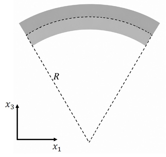
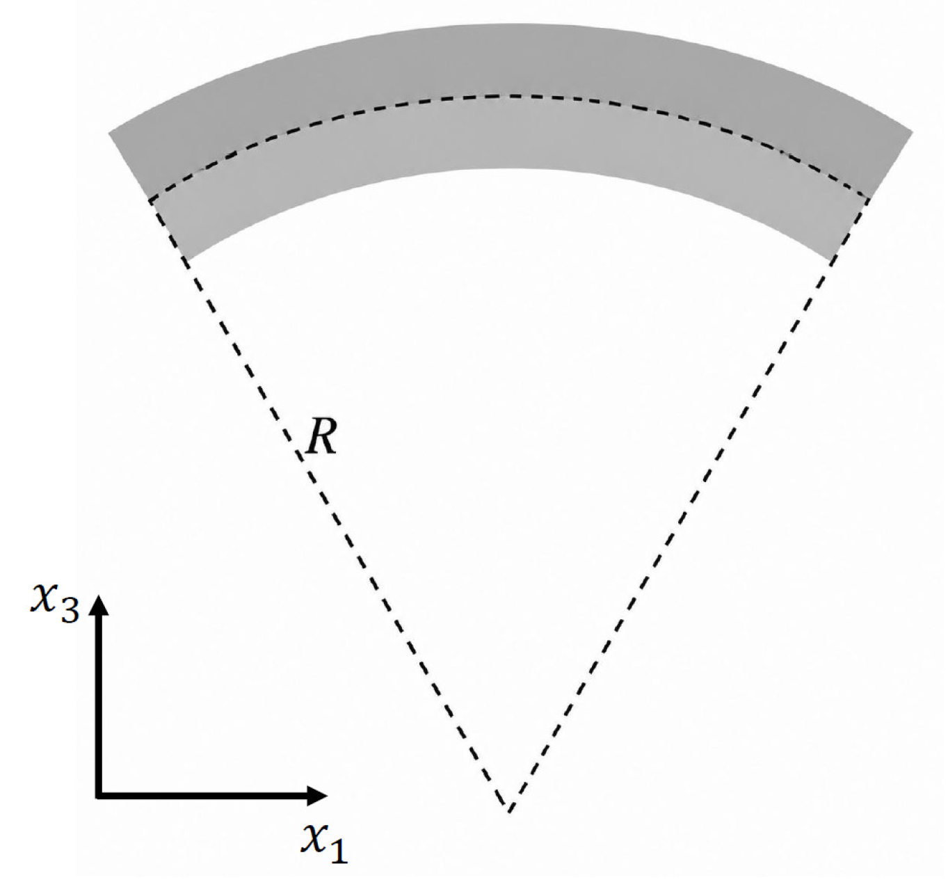
To exemplify wrinkled laminates, in Figure 1, we consider the geometry of a strain gradient produced in a layer described by

$$x_3=f(x_1)$$

with local radius, R. The radius is related to f by

$$R={\displaystyle \frac{{(1+f^{\prime 2})}^{3/2}}{|f^{″}|}}$$

where $\prime ={\partial }_{x_1}$. For small values of the slope, $f^{\prime 2}\ll 1$, we have

$$R\simeq {\displaystyle \frac{1}{|f^{″}|}}={\displaystyle \frac{1}{|{\partial }_{x_1}^2{x}_3|}}$$

Hence, we obtain the polarization in terms of the radius and the flexoelectric coefficient,

$${\displaystyle \frac{1}{\rho }}{P}_3={\displaystyle \frac{1}{2R}}\mathcal{F}.$$

Figure 1. An example of a strain gradient parameterized by the radius of a laminate.

4.3. Remarks on Flexoelectric Coefficients

According to (26), if $\mathbf{E}=\mathbf{0}$, then

$${\displaystyle \frac{1}{\rho }}{P}_q=-e_{qjk}{\mathcal{E}}_{jk}+{\mathcal{F}}_{qQjk}{\mathcal{E}}_{jk,Q},$$

represents piezoelectricity and flexoelectricity, namely the polarization induced by strain and the strain gradient, respectively. In connection with flexoelectricity, a wide range of activities have been performed to determine the flexoelectric coefficient through various methods, all of them involving various techniques for the generation of strain gradients. In this respect, I mention [22,23] and the references therein. In particular, Table 1 of [22] provides methods, values and specific references for measuring the flexoelectric coefficients of biological materials. An analogous Table 1 is established in [23], where the coefficients and the adopted methods are given for various materials, particularly ceramics.

The values of $\mathcal{F}$ for flexoelectric materials range from ${10}^{-9}$ to ${10}^{-4}$ C/m. While, e.g., the value of $\mathcal{F}$ is about ${10}^{-9}$ C/m for graphene, the best performances are found in the ceramic material BaSrTiO₃ (Barium Strontium Titanate, or BST). Furthermore, in Nb-doped ${\mathrm{TiO}}_2$, it is $\mathcal{F}\simeq {10}^{-3}$ C/m (see Figure 6 of [23]), depending on the thickness of the layer.

The main feature of the present description of flexoelectric materials is the thermodynamic consistency, derived through the CD inequality, of the dependence of higher-order spatial derivatives. Meanwhile, the scheme allows for the identification of dissipative effects through $\mathcal{T}$ and $\mathcal{P}$, as is specified in the next section. On the whole, non-locality is mathematically consistent with CD inequality through the extra-entropy flux $\mathbf{k}$, while the dissipative character of stress and polarization is provided by the entropy production, $\gamma$.

5. Representations of $\mathcal{T}$ and $\mathcal{P}$

The consequences of the reduced CD inequality (20) on the constitutive functions, ${\mathcal{T}}^{sym},\mathcal{P},\mathbf{{\rm Y}},$ and $\mathbf{q}$, are investigated by using a general representation formula for obtaining a solution to equations involving inner products of tensors or vectors.

Let $\mathbf{v}$ be a non-zero vector and $\mathbf{e}$ the unit vector $\mathbf{e}=\mathbf{v}/\left|\mathbf{v}\right|$. Any vector, $\mathbf{g}$, can be represented as

$$\mathbf{g}=(\mathbf{g}·\mathbf{e})\mathbf{e}+{\mathbf{g}}_{\perp },$$

where ${\mathbf{g}}_{\perp }$ is orthogonal to $\mathbf{e}$ in that ${\mathbf{g}}_{\perp }·\mathbf{e}=0$. Indeed,

$${\mathbf{g}}_{\perp }=\mathbf{g}-(\mathbf{g}·\mathbf{e})\mathbf{e}=(\mathbf{1}-\mathbf{e}\otimes \mathbf{e})\mathbf{g}.$$

Notice that, for any vector, $\mathbf{p}$,

$$(\mathbf{1}-\mathbf{e}\otimes \mathbf{e})\mathbf{p}$$

is orthogonal to $\mathbf{e}$. Hence, if the transverse part, ${\mathbf{g}}_{\perp }$, of $\mathbf{g}$ is undetermined, then the vector, $\mathbf{g}$, can be represented as

$$\mathbf{g}=(\mathbf{g}·\mathbf{e})\mathbf{e}+(\mathbf{1}-\mathbf{e}\otimes \mathbf{e})\mathbf{p},$$

with $\mathbf{p}$ as an arbitrary vector. Hence, in terms of the vector $\mathbf{w}$, we have

$$\mathbf{g}={\displaystyle \frac{\mathbf{g}·\mathbf{v}}{{\left|\mathbf{v}\right|}^2}}\mathbf{v}+(\mathbf{1}-{\displaystyle \frac{\mathbf{v}\otimes \mathbf{v}}{{\left|\mathbf{v}\right|}^2}})\mathbf{p}.$$

(27)

A strict analogue holds for tensors. For any tensor, $\mathbf{\Lambda }$, let $\left|\mathbf{\Lambda }\right|={(\mathbf{\Lambda }·\mathbf{\Lambda })}^{1/2}$. A tensor $\mathbf{A}$ can be split in the form

$$\mathbf{A}={\displaystyle \frac{\mathbf{A}·\mathbf{\Lambda }}{{\left|\mathbf{\Lambda }\right|}^2}}\mathbf{\Lambda }+(\mathsf{I}-{\displaystyle \frac{\mathbf{\Lambda }\otimes \mathbf{\Lambda }}{{\left|\mathbf{\Lambda }\right|}^2}})\mathbf{A},$$

where $\mathsf{I}$ is the fourth-order identity tensor. If the transverse part, with respect to $\mathbf{\Lambda }$, is undetermined, then any representation of $\mathbf{A}$,

$$\mathbf{A}={\displaystyle \frac{\mathbf{A}·\mathbf{\Lambda }}{{\left|\mathbf{\Lambda }\right|}^2}}\mathbf{\Lambda }+(\mathsf{I}-{\displaystyle \frac{\mathbf{\Lambda }\otimes \mathbf{\Lambda }}{{\left|\mathbf{\Lambda }\right|}^2}})\mathbf{B},$$

(28)

holds with $\mathbf{B}$, or any arbitrary tensor.

Let $(\mathbf{z},\mathbf{v})$ be the set of variables. Assume the CD inequality implies a relation in the form

$$\mathbf{g}·\mathbf{v}=f(\mathbf{z},\mathbf{v})$$

with $\mathbf{g}$ as the unknown vector function and f as a scalar-valued function. Hence, the representation (27) yields

$$\mathbf{g}={\displaystyle \frac{f}{{\left|\mathbf{v}\right|}^2}}\mathbf{v}+(\mathbf{1}-{\displaystyle \frac{\mathbf{v}\otimes \mathbf{v}}{{\left|\mathbf{v}\right|}^2}})\mathbf{p}.$$

(29)

A sufficient condition for the validity of the reduced CD inequality (20) is the assumption that each power satisfies a proper reduced CD inequality,

$${\mathcal{T}}^{sym}·\dot{\mathcal{E}}=\rho \theta {\gamma }_T,\mathcal{P}·\dot{\mathbf{E}}=\rho \theta {\gamma }_E,\mathbf{{\rm Y}}·\varkappa =\rho \theta {\gamma }_{\mathrm{{\rm Y}}},\mathbf{q}·\nabla \theta =\rho {\theta }^2{\gamma }_q.$$

Consider the inequality for ${\mathcal{T}}^{sym}$. Using the representation formula (28) with the identifications $\mathbf{A}={\mathcal{T}}^{sym}$ and $\mathbf{\Lambda }=\dot{\mathcal{E}}$ or $\mathbf{g}=\mathcal{P}$ and $\mathbf{v}=\dot{\mathbf{E}}$, we obtain

$${\mathcal{T}}^{sym}={\displaystyle \frac{\rho \theta {\gamma }_T}{|\dot{\mathcal{E}}{|}^2}}\dot{\mathcal{E}}+(\mathsf{I}-{\displaystyle \frac{\dot{\mathcal{E}}\otimes \dot{\mathcal{E}}}{|\dot{\mathcal{E}}{|}^2}})\mathbf{B}$$

(30)

and

$$\mathcal{P}={\displaystyle \frac{\rho \theta {\gamma }_E}{|\dot{\mathbf{E}}{|}^2}}\dot{\mathbf{E}}+(\mathbf{1}-{\displaystyle \frac{\dot{\mathbf{E}}\otimes \dot{\mathbf{E}}}{|\dot{\mathbf{E}}{|}^2}})\mathbf{p}.$$

(31)

The splitting of ${\mathcal{T}}^{sym}$ or $\mathcal{P}$ on the right-hand side allows the first term to be viewed as the dissipative part in that the coefficient is proportional to the corresponding entropy production, ${\gamma }_T$ or ${\gamma }_E$. The second term is geometrically transverse to $\dot{\mathcal{E}}$ or $\dot{\mathbf{E}}$ and is non-dissipative in that it provides a zero term for the power ${\mathcal{T}}^{sym}·\dot{\mathcal{E}}$ or $\mathcal{P}·\dot{\mathbf{E}}$. In general, for constitutive functions occurring in the CD inequality through an inner product, the general solution is a dissipative term along the power conjugate ($\dot{\mathcal{E}}$ or $\dot{\mathbf{E}}$) and any transverse term, relative to the power conjugate. For example, letting $\mathbf{p}=\lambda \nabla \theta$, we have

$$\mathcal{P}={\displaystyle \frac{\rho \theta {\gamma }_E}{|\dot{\mathbf{E}}{|}^2}}\dot{\mathbf{E}}+\lambda {(\nabla \theta )}_{\perp },{(\nabla \theta )}_{\perp }=\nabla \theta -(\nabla \theta ·\dot{\mathbf{E}}/|\dot{\mathbf{E}}{|}^2)\dot{\mathbf{E}}.$$

The dependence on any transverse part is usually ignored in the literature.

As is apparent from (30) and (31), the constitutive equations for the dissipative terms, ${\mathcal{T}}^{sym},\mathcal{P}$, are affected by the form of the entropy productions, ${\gamma }_T,{\gamma }_E$. This emphasizes the consistency and generality of allowing the entropy production, $\gamma$, to be given by a constitutive equation [3].

6. Dynamic Equations

As shown in Section 4 and Section 5, once the electric enthalpy, $\varphi$, and the entropy production, $\gamma$, are selected, the thermodynamic relations (21) and (22) determine the constitutive functions of ${\mathbf{T}}^{sym}$ and $\mathbf{P}$. To fix these ideas, we let the material be polar ($\mathbf{P}\times \mathbf{E}\ne \mathbf{0}$) but not micropolar ($\mathbf{l}=\mathbf{0}$). Hence, to describe the dynamics of the body, we apply the balance Equations (5), (A1), (A2) and (A5). Consequently, we need the entire stress tensor, $\mathbf{T}={\mathbf{T}}^{sym}+{\mathbf{T}}^{skw}$.

By condition (A5), we have

$$\mathbf{{\rm Y}}=-\mathbf{c},{\mathrm{{\rm Y}}}_i={ϵ}_{ikj}{T}_{jk}.$$

(32)

Since

$${ϵ}_{pqi}{\mathrm{{\rm Y}}}_i={ϵ}_{pqi}{ϵ}_{ikj}{T}_{jk}=({\delta }_{pk}{\delta }_{qj}-{\delta }_{pj}{\delta }_{qk})T_{jk}=T_{qp}-T_{pq}=2T_{qp}^{skw}$$

then

$$T_{qp}^{skw}=-\frac{1}{2}{ϵ}_{qpi}{\mathrm{{\rm Y}}}_i=\frac{1}{2}{ϵ}_{qpi}{c}_i.$$

Once the body couple $\mathbf{c}$ is known, ${\mathbf{T}}^{skw}$ is given by (6). If, as in dielectrics, $\mathbf{c}=\mathbf{P}\times \mathbf{E}$, then Equation (32) implies that

$${ϵ}_{ikj}{T}_{jk}=-{ϵ}_{ijk}{P}_j{E}_k$$

whence

$${ϵ}_{ijk}(T_{kj}+E_k{P}_j)=0,\mathrm{skw}(\mathbf{T}+\mathbf{E}\otimes \mathbf{P})=\mathbf{0},$$

$${\mathbf{T}}^{skw}=\frac{1}{2}(\mathbf{P}\otimes \mathbf{E}-\mathbf{E}\otimes \mathbf{P}).$$

(33)

The required constitutive equations for $\mathbf{T}$ and $\mathbf{P}$ are then given by (21), (22), and (33).

7. Conclusions

This paper addresses the models of dielectric materials with higher-order gradients and, in particular, flexoelectric materials. While the literature develops the subject through variational formulation, here the modelling is examined within a thermodynamic framework.

Owing to flexoelectricity, the dielectric material has a polar character in that the polarization, $\mathbf{P}$, need not be parallel to the electric field, $\mathbf{E}$, and then a non-zero body couple, $\mathbf{c}=\mathbf{P}\times \mathbf{E}$, happens. Accordingly, the balance equations are revisited and the joint occurrence of ${\mathbf{T}}^{skw}$ and $\mathbf{c}$ is restated in the balance of angular momentum.

The stress power is taken in the simple form, $\mathbf{T}·\mathbf{L}$, without any use of hyper-stresses or recourse to the principle of virtual work. Consistent with the modelling via strain gradient, the stretching, $\mathbf{D}=\mathrm{sym}\mathbf{L}$, is approximated with the strain rate, $\dot{\mathcal{E}}=\mathrm{sym}\dot{\mathbf{H}}$, which holds for small values of the displacement gradient, $\left|\mathbf{H}\right|\ll 1$. Hence, it follows that ${\mathbf{T}}^{sym}$ and $\mathbf{P}$ are given by the variational derivatives, ${\delta }_{\mathcal{E}}\varphi$ and ${\delta }_{\mathbf{E}}\varphi$, to within the dissipative parts, ${\mathcal{T}}^{sym}$ and $\mathcal{P}$ (Equations (18) and (19)). Hence, the model of ${\mathbf{T}}^{sym}$ and $\mathbf{P}$ is established once we select the electric enthalpy, $\varphi$. These results holds thanks to an appropriate expression of the extra-entropy flux, $\mathbf{k}$, while the entropy production, $\gamma$, enters the dissipative parts, ${\mathcal{T}}^{sym}$ and $\mathcal{P}$. Furthermore, ${\mathbf{T}}^{skw}$ in a polar material is free from thermodynamic requirements and is determined by (33) to counterbalance the action of the body couple. Instead, in a micropolar model, ${\mathbf{T}}^{skw}$ is subject to a thermodynamic requirement in the form $\mathbf{{\rm Y}}·\varkappa =\rho \theta {\gamma }_{\mathrm{{\rm Y}}}$; both the body couple and the skewed part of the stress determine the evolution of the internal spin vector, $\mathbf{l}$.

References

- Coleman, B.D.; Noll, W. The thermodynamics of elastic materials with heat conduction and viscosity. Arch. Ration. Mech. Anal. 1963, 13, 167–178. [Google Scholar] [CrossRef] [Scilit]
- Müller, I. On the entropy inequality. Arch. Ration. Mech. Anal. 1967, 26, 118–141. [Google Scholar] [CrossRef] [Scilit]
- Morro, A. Thermodynamically consistent evolution equations in continuum mechanics. Foundations 2024, 4, 494–512. [Google Scholar] [CrossRef] [Scilit]
- Giorgi, C.; Morro, A. Second law of thermodynamics and strain gradient theories of elasticity. Entropy 2026, 28, 487. [Google Scholar] [CrossRef] [Scilit] [PubMed]
- Giorgi, C.; Morro, A. A thermodynamic approach to rate-type models of elastic-plastic materials. J. Elast. 2021, 147, 113–148. [Google Scholar] [CrossRef] [Scilit]
- Giorgi, C.; Morro, A. Thermodynamically-consistent modeling of ferromagnetic hysteresis. Materials 2023, 16, 2882. [Google Scholar] [CrossRef] [Scilit] [PubMed]
- Germain, P. La méthode des puissances virtuelles en mécanique des mileux continus. Première partie: Theorie du second gradient. J. Mécanique 1973, 12, 235–274. [Google Scholar]
- Hadjesfandiari, A.R.; Dargush, G.F. Couple stress theory for solids. Int. J. Solds Struct. 2011, 48, 2496–2510. [Google Scholar] [CrossRef] [Scilit]
- Hu, T.; Yang, W.; Liang, X.; Shen, S. Wave propagation in flexoelectric microstructured solids. J. Elast. 2018, 130, 197–210. [Google Scholar] [CrossRef] [Scilit]
- Li, A.; Zhou, S.; Qi, I.; Chen, X. A flexoelectric theory with rotation gradient effects for elastic dielectrics. Model. Simul. Mater. Sci. Eng. 2016, 24, 0155009. [Google Scholar] [CrossRef] [Scilit]
- Behera, A.K.; Pillai, A.U.; Das, A.; Rahaman, M.M. A micropolar phase-field model for size-dependent electro-mechanical fracture. Int. J. Mech. Sci. 2025, 285, 109805. [Google Scholar] [CrossRef] [Scilit]
- Gurtin, M.E.; Fried, E.; Anand, L. The Mechanics and Thermodynamics of Continua; Cambridge University Press: New York, NY, USA, 2011. [Google Scholar]
- Morro, A.; Giorgi, C. Mathematical Modelling of Continuum Physics; Birkhäuser: Cham, Swizerland, 2023. [Google Scholar]
- Zemansky, M.W.; Dittman, R.H. Heat and Thermodynamics; McGraw-Hill: New York, NY, USA, 1997. [Google Scholar]
- Truesdell, C. Rational Thermodynamics; Springer: New York, NY, USA, 1984. [Google Scholar]
- Dreyer, W.; Kunik, M. Maximum entropy principle revisited. Cont. Mech. Thermodyn. 1998, 10, 331–347. [Google Scholar] [CrossRef] [Scilit]
- Gonzalez-Narvaez, R.E.; Vázquez, F.; López de Haro, M. Validity of Prigogine’s minimum entropy production principle for a rigid heat-conducting solid beyond the Fourier heat transport regime. Cont. Mech. Thermodyn. 2022, 34, 1553–1561. [Google Scholar] [CrossRef] [Scilit]
- Dyke, J.; Kleidon, A. The Maximum entropy production principle: Its theoretical foundations and applications to the earth systems. Entropy 2010, 12, 613–630. [Google Scholar] [CrossRef] [Scilit]
- Gupta, M.; Pingale, A.D.; Kundalwal, S.I. Continuum and computational modeling of flexoelectricity in nanomaterials: A review. J. Appl. Phys. 2025, 138, 190702. [Google Scholar] [CrossRef] [Scilit]
- Gao, X.-L.; Park, S. Variational formulation of a simplified strain gradient elasticity theory and its application to a pressurized thick-walled cylinder problem. Int. J. Solids Struct. 2007, 44, 7486–7499. [Google Scholar] [CrossRef] [Scilit]
- Kalinin, S.V.; Meunier, V. Electronic flexoelectricity in low-dimensional systems. Phys. Rev. B 2008, 77, 033403. [Google Scholar] [CrossRef] [Scilit]
- Mohammadkhah, M.; Slavkovich, V.; Klinge, S. Flexoelectricity in biological materials and its potential applications in biomedical research. Bioengineering 2025, 12, 579. [Google Scholar] [CrossRef] [Scilit] [PubMed]
- Kolodziej, M.; Ojha, N.; Budziałowski, M.; Załęski, K.; Fina, I.; Mishra, Y.K.; Pant, K.K.; Coy, E. CoyFundamentals of flexoelectricity, materials and emerging opportunities toward strain-driven nanocatalysts. Small 2024, 20, 2406726. [Google Scholar] [CrossRef] [Scilit] [PubMed]
Disclaimer/Publisher’s Note: The statements, opinions and data contained in all publications are solely those of the individual author(s) and contributor(s) and not of MDPI and/or the editor(s). MDPI and/or the editor(s) disclaim responsibility for any injury to people or property resulting from any ideas, methods, instructions or products referred to in the content. |
© 2026 by the author. Licensee MDPI, Basel, Switzerland. This article is an open access article distributed under the terms and conditions of the Creative Commons Attribution (CC BY) license.