


Abstract
The accurate quantification of microplastics (MPs) in aquatic environments remains challenging due to the heterogeneous distribution of MPs in different environments, making representative sampling difficult, as well as methodological variabilities in sampling, sample processing, and detection. This study examined measurement fluctuations for MP analysis across four distinct water matrices: wastewater treatment plant (WWTP) effluent, tap water (TW), combined sewer overflow (CSO), and surface water (SW). Two sampling strategies were compared: grab sampling (0.5 L, n = 5) and large-volume filtration using a particle sampling unit (PSU; 100 L, 10 µm mesh, subsampled). Samples were processed through oxidative digestion, stained with fluorescent dye, and analyzed via fluorescence microscopy with automated particle counting. Recovery experiments using polyamide (PA) reference particles (357 ± 60 µm) were conducted to assess method accuracy. PSU sampling demonstrated higher precision (mean R.S.D. 41 ± 17%) compared to grab sampling (mean R.S.D. 64 ± 19%), despite additional variability introduced by subsampling. Recovery rates reached 93 ± 7% for grab samples and 88 ± 23% for PSU samples with complete filter analysis. Statistical modeling revealed that achieving a ±25% margin of error (95% CI) required 21 PSU samples versus 51 grab samples. The quadratic relationship between the margin of error and required sample size underscores the importance of methodological optimization for cost-effective monitoring. These findings provide practical guidance for designing MP monitoring campaigns and demonstrate that fluorescent labeling combined with large-volume sampling offers a reliable approach for MP quantification in diverse aquatic environments.
1. Introduction
Microplastics (MPs), defined as plastic particles smaller than 5 mm, are ubiquitous and persistent contaminants in freshwater and marine environments, raising concerns regarding ecosystem and human health [1,2,3,4,5]. The continuous influx of primary MPs and the continuous generation of secondary MPs through the fragmentation of larger plastic debris, in combination with their slow degradation, contribute to their progressive accumulation across all environmental compartments [1,6,7]. MP detection is fundamental for environmental monitoring, risk assessment, and the development of effective mitigation strategies. However, despite more than a decade of intensive research since the term ‘microplastic’ was introduced by Thompson and colleagues in 2004, significant methodological challenges persist that compromise data comparability and reliability across studies [8,9,10,11].
MP sampling and detection comprises three main steps—collection, preparation, and analysis—and is complicated by the vast diversity of polymer types, particle shapes, and size ranges present in environmental samples [12,13]. The primary methods used for collecting water samples are net sampling, bulk water or grab sampling with subsequent filtration, and pump filtration, each with limitations and advantages, as outlined in Table 1. For wastewater treatment plants (WWTPs), pump and grab sampling are the most feasible methods and enable the detection of a wider range of MP sizes.
Table 1.
Primary methods for MP sample collection from water [14,15].
Another major challenge is the distinction of synthetic polymers from natural organic matter, such as lignin, cellulose, or chitin, which can exhibit similar physical and chemical properties, leading to false positives or signal interference. Selective separation and detection strategies that reliably distinguish plastics from biogenic particles are thus essential.
The accurate detection of MPs requires a systematic sample preparation protocol to isolate plastic particles from complex environmental matrices [12,13,16]. The processing of water samples typically begins with filtration, using sieves or membrane filters to retain particles within the MP size range. This is followed by chemical digestion, where organic matter is removed through oxidative agents such as hydrogen peroxide or enzymatic treatments. If necessary, density separation is employed, suspending the sample in a high-density solution (e.g., sodium iodide or zinc chloride), allowing plastic particles to float while heavier materials, mainly minerals, settle [12,13,16]. Despite these established steps, the field lacks standardized, harmonized protocols—a gap that significantly limits data comparability and our understanding of the true extent of MP pollution [15,17].
Thus, quality assurance and quality control (QA/QC) represent critical yet often inadequately addressed aspects of MP analysis [11,18]. Hermsen et al. (2018) conducted a comprehensive critical review of quality criteria for MP analysis in biota samples, proposing a scoring method based on ten criteria, including the sampling strategy, the sample size, laboratory preparation, clean air conditions, negative and positive controls, sample treatment, and polymer identification [11]. Their assessment revealed a strong need for stricter quality assurance, with only three studies including reliable positive controls [15,17].
Recovery rate determination through spiking experiments represents a cornerstone of analytical method validation yet remains inconsistently implemented in MP research. Way et al. (2022) reported average underestimation of 14% across multiple recovery studies reviewed and showed that recovery also depends on the sample matrix [19].
The sampling process itself introduces significant sources of error that are frequently overlooked in recovery rate assessments. Weber and Kerpen (2023) conducted one of the first comprehensive investigations of MP recovery rates, including sampling, sample preparation, subsampling, and detection under near-realistic experimental conditions [20]. Using volume-reduced sampling from an experimental flume simulating WWTP effluents, they determined average recovery rates of only 27 ± 10% for polypropylene MP particles (d = 53 ± 29 µm), with the smallest size fraction (<50 µm) showing recovery rates as low as 9%. For denser polyvinyl chloride particles (d = 151 ± 37 µm), the recovery rates reached 78 ± 14%. These findings strongly suggest that MP emissions, particularly from point sources such as WWTPs, may be substantially underestimated.
Subsampling strategies have emerged as a critical consideration for efficient and accurate MP quantification, particularly when dealing with samples containing high particle numbers. De Frond et al. (2023) established best practices for the representative subsampling of MPs for chemical identification, emphasizing that subsampling methods are driven by research objectives [21]. Their analysis revealed that fewer particles are required to identify the number of plastic particles in the sample, while a higher number of particles needs to be analyzed to representatively characterize the proportions of polymer types. Because no standardized subsampling protocols currently exist, methods vary widely and often lack evidence of representativeness, limiting conclusions and cross-study comparability.
Procedural contamination remains a challenge in MP analysis due to the ubiquitous presence of synthetic particles in laboratory environments. Munno et al. (2023) analyzed blank contamination patterns from 12 participating laboratories and found MP contamination ranging from 7 to 511 particles per sample, with a mean of 80 particles (±SD 134) [22]. The most common morphology reported was black fibers in the 20–212 µm size fraction. Brander et al. (2020) provided comprehensive guidance on sampling and quality assurance procedures, recommending that researchers implement good laboratory practices including air filtration, filtered water usage, non-synthetic clothing policies, and enclosed airflow systems to minimize secondary contamination [23].
Spectroscopic techniques, particularly Fourier-transform infrared (FTIR) and Raman microspectroscopy, are widely used as analytical detection techniques for the chemical identification of MPs [24,25]. Focal plane array-based micro-FTIR imaging has enabled the automated identification of MPs concentrated on filter membranes without presorting, providing considerable reductions in analysis times and increased accuracy through the impartial measurement of entire filter surfaces [26]. Raman spectroscopy offers a superior spatial resolution (down to 1 µm compared to FTIR’s 10–20 µm) and reduced interference from water, making it particularly suitable for analyzing smaller MP particles [27,28]. These deliver precise polymer identification but demand long processing times and specialized equipment and are sensitive to interference by chemical transformations of the plastic surfaces in the environment. Another commonly applied method is pyrolysis–gas chromatography–mass spectrometry (Py-GC-MS), which enables the polymer-specific identification and quantification of MPs [29]. While highly specific and capable of analyzing mixed polymers without prior sorting, the method is destructive and provides no information on particle size or morphology [30,31,32]. Furthermore, it suffers from high acquisition and maintenance costs and requires specialized, well-trained operators. These limitations lead to high costs and time requirements for MP monitoring, making comprehensive sampling campaigns with large sample sizes for MP analytics less viable. This has driven the development of rapid, cost-effective methods suitable for large-scale monitoring workflows.
The fluorescent staining of MPs has emerged as an attractive solution to these challenges, enabling the rapid visualization and quantification of MPs [33,34]. It was established with fluorescent dyes such as Nile red and later with improved derivatives that selectively adsorb onto polymer surfaces, producing strong fluorescence signals under specific excitation wavelengths [35]. This approach reduces background interference by discriminating stained plastics from organic or mineral particles, which show a weaker or no fluorescence signal. It enables automated image analysis for MP detection based on brightness thresholds [36]. Crucially, fluorescence-based methods can be implemented with affordable fluorescence microscopes, lowering technical barriers. Another advantage is the short imaging and processing time, allowing a high sample throughput. However, strong fluorescence from natural particles can lead to false positives. Extensive sample preparation is therefore required to reduce interference from these naturally occurring particles by completely degrading them or wakening their fluorescence signals [35].
Sturm et al. (2023) introduced a standardized fluorescence-based MP detection method employing a proprietary stain mix (MP-1) containing optimized Nile red derivatives [37]. The workflow involves the hydrogen peroxide digestion of organic matter, followed by staining with abcr eco Wasser 3.0 detect mix MP-1 (AB930015, abcr GmbH, Karlsruhe, Germany) under a controlled temperature for sample preparation. For detection, fluorescence imaging using tailored bandpass filters is applied. Automated MP detection via brightness thresholds and counting enhances reproducibility and reduces the processing time per sample. Thus, the time from a sample entering the lab until the results are available is approximately 2.5 h, of which, depending on the sample, approximately 30 min of pure working time is required for sampling, sample processing, imaging, and image analysis [38,39].
Comparing, validating, and evaluating different MP detection protocols against each other requires method validation according to established analytical criteria [40]. This is particularly important for MP analysis, as sampling and sample preparation are highly error-prone due to the heterogeneous distribution of MPs, which vary widely in density, size, and shape. This study addresses these knowledge gaps by comparing two sampling approaches for MPs in different water types using both large and small sample volumes. Sample processing involves standardized hydrogen peroxide digestion followed by fluorescence-based MP detection. Known quantities of reference MPs are spiked into various water samples and precision is assessed through recovery rate analyses and by evaluating measurement variability arising from repeated sampling and sample processing. Overall, this work contributes to ongoing efforts to establish robust, reproducible, and internationally harmonized methods for MP analysis, supporting reliable environmental monitoring and risk assessment.
2. Materials and Methods
2.1. Sampling Sites
WWTP samples were collected at the outlet of the WWTP Landau-Mörlheim, a municipal WWTP with three treatment stages (mechanical, biological, and phosphate removal) and a capacity of 80,000 population equivalents (PE).
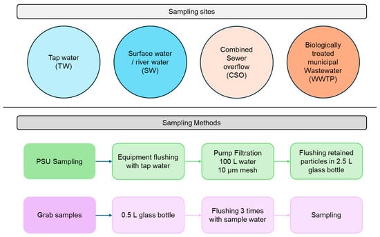
Tap water (TW) samples were collected at the TW connection of the WWTP Landau-Mörlheim. The combined sewer overflow (CSO) is located at the inlet of the WWTP and fills during heavy rain events, which leads to inflowing volumes exceeding the capacity of the WWTP. The CSO is filled with a mix of rainwater and sewage water. Surface water (SW) sampling is conducted at the River Queich, approximately 400 m downstream of the WWTP effluent. Table 2 summarizes the sampling sites and GPS coordinates, and Figure 1 provides an overview of the sampling sites and the sample methods (described in Section 2.2).
Table 2.
Sampling locations, their abbreviations, and GPS coordinates (WGS 84).
Figure 1.
Overview of the sampling sites and methods.
The differences among these water types lie in the concentrations and compositions of suspended particulate matter. Wastewater typically contains high loads of organic sludge residues, CSO includes substantial amounts of road-derived particulates and urban runoff mixed with untreated wastewater, river water carries mineral sediments but also organic residues, and TW contains only minimal particulate content due to prior treatment.
2.2. Sample Collection
2.2.1. PSU Samples—Pump Filtration Through Filter Cartridge
Particle sampling unit (PSU) sampling was performed following the protocol established by Sturm et al. (2024) [41]. The PSU is a compact system composed of a 10 µm filter cartridge (01WTGD, Wolftechnik Filtersysteme GmbH & Co., KG, Weil, Germany) integrated with a pump (MG80B C-B-CMS1B, Grundfos, Erkrath, Germany), hoses, valves, and a water meter [41]. The sampled water flows through the filter cartridge under a maximum pressure of 4 bar. All particles larger than 10 µm, including MPs, are retained by the filter, while smaller particles and water are discharged.
The inlet hose (black polyvinyl chloride) is equipped with a suction basket and positioned centrally within the sampled water. The outlet hose is placed downstream of the inlet, aligned with the flow direction. Prior to each sampling event, the PSU is flushed with tap water to prevent cross-contamination.
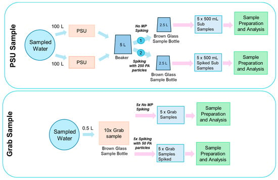
For each PSU sampling, two 100 L samples were taken, equating to a total volume of 200 L of water filtered. This resulted in volumetric loading of 60.1 for the used filter cartridge. Following filtration, the filter cartridge was removed from the housing, and retained solids were rinsed into a 2.5 L glass bottle (AB258145, abcr GmbH, Karlsruhe, Germany) using a spray bottle. After this, both samples were merged and mixed in a 5 L beaker. Using a scale, the samples were divided evenly into two 2.5 L glass bottles by alternating pouring. This was performed to prevent particles from sticking to the volumetric cylinder, which would otherwise be needed to divide the 5 L evenly by volume. To achieve as even a distribution as possible, the 5 L beaker cup was not flushed after pouring. Therefore, some of the particles and MPs remained stuck to the beaker. The 2.5 L glass bottles for sample storage had black PE bottle caps with a Teflon-coated PE foam seal. The collected samples were then transported to the laboratory for subsequent processing and analysis.
For the sampling of the CSO, the water was previously filled into an international bulk container (IBC). Since heavy rain events, which cause the CSO tank to overflow, typically occur spontaneously and unpredictably, filling the water into an IBC allows for quick and spontaneous sampling, as it requires little time and preparation. The sample (500–700 L) can then be stored. When the PSU sample is subsequently taken from the IBC, it is continuously mixed by an agitator, and the PSU is connected to the IBC outlet.
For TW sampling, the inlet hose was directly connected to the tap.
2.2.2. Grab Samples
Grab samples were collected using 0.5 L brown glass bottles (Rixius GmbH, Mannheim, Germany). Prior to sample collection, each bottle was rinsed three times with the sampled water to minimize contamination. Subsequently, the bottles were filled with water and sealed immediately. Sample bottle caps were equipped with Teflon-coated liners to prevent chemical interference (Rixius GmbH, Mannheim, Germany). Ten grab samples were taken subsequently for each sample site. All samples were stored at room temperature (RT) until further analysis.
2.2.3. Spiking with PA-Based Microplastics
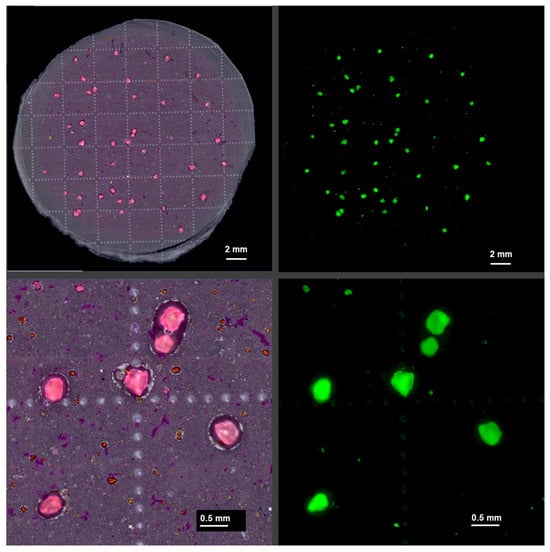
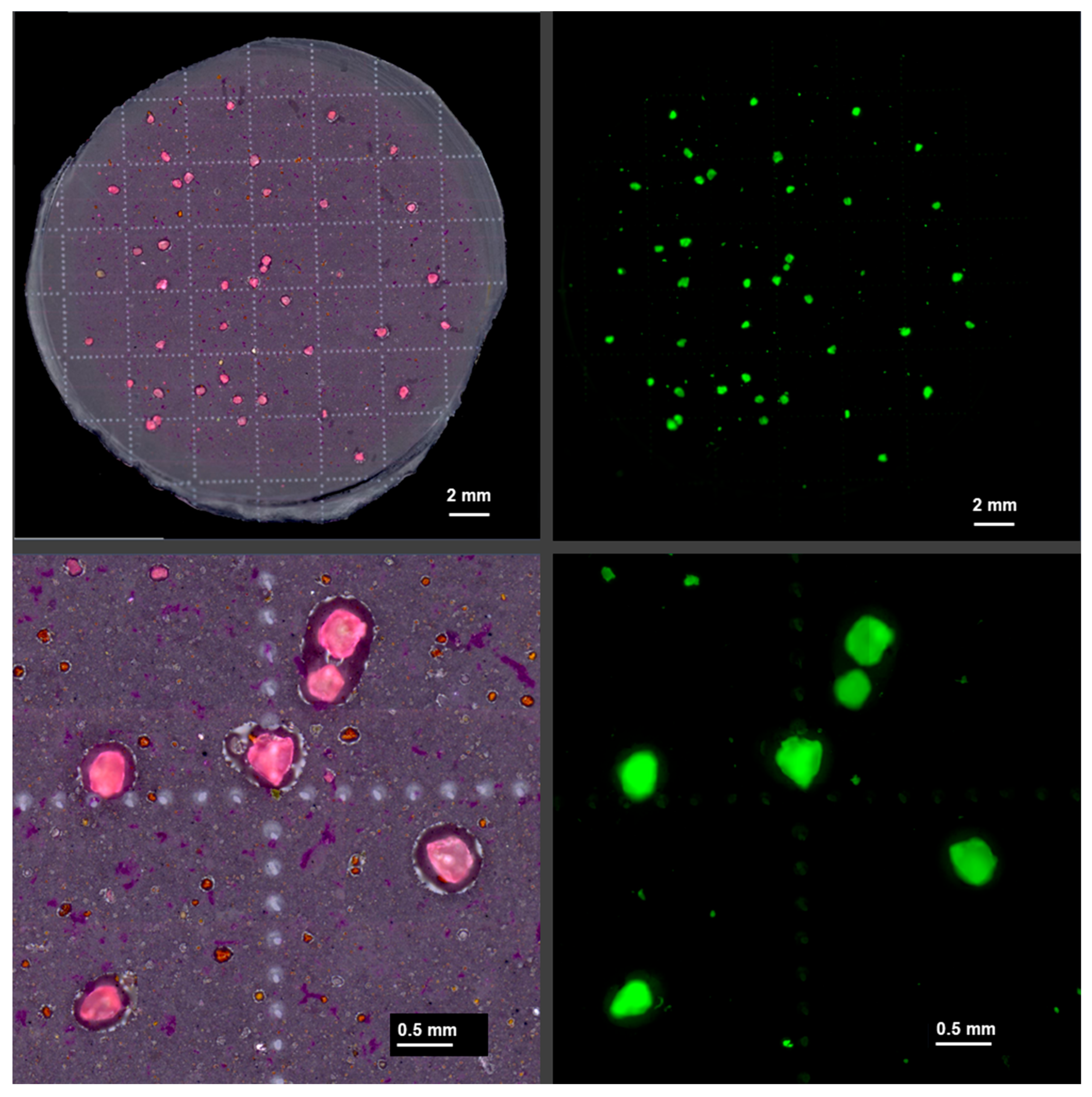
To evaluate recovery rates across different aquatic environments, polyamide (PA, EMS-Grilltech, Domat/Ems, Switzerland) granules were spiked into the samples (Figure 2). Due to their distinctive shape, bright pink color, and size, these granules are easily identifiable, allowing straightforward visual identification in light microscopy images (Figure 3). In the visual inspection of non-spiked control samples, these particles were absent. The mean size of the particles was 357 ± 60 µm, determined microscopically by measuring 10 particles. Five of the ten grab samples were spiked, adding 50 PA particles per sample into the sample bottle. For the PSU samples of each respective sampling site, 250 particles were spiked into one of the two 2.5 L sample bottles derived from the 100 L samples, while the other bottle remained unspiked (Figure 2). This allowed us to evaluate the accuracy of the subsampling process.
Figure 2.
Overview of the sampling process with different sample volumes, spiking, and evaluation.
Figure 3.
Color images (left) and corresponding fluorescence images (right, green channel) of a spiked CSO grab sample. The relatively large spiked PA particles are easily identified due to their size, shape, and strong pink color after staining.
2.3. Sample Processing
In the laboratory, all samples were initially filtered using a 10 µm stainless-steel filter (Wolftechnik Filtersysteme GmbH & Co. KG, Weil, Germany). For PSU samples, 500 mL subsamples were taken from the original 2.5 L volume by shaking it for 30 s and pouring 500 mL into a volumetric cylinder. This resulted in 5 subsamples per 2.5 L sample bottle. For the grab samples, the whole sample was filtered. Subsampling was implemented because the original 2.5 L PSU sample caused filter clogging during laboratory vacuum filtration. A reduced volume of 0.5 L was identified as the maximum amount that could be reliably filtered without excessive clogging.
The filter containing retained particulate matter was transferred to a glass beaker and further processed with oxidative digestion to eliminate organic material while preserving synthetic polymer particles. Digestion was performed using 35% hydrogen peroxide (H2O2; AB171423, abcr GmbH, Karlsruhe, Germany) in combination with iron(II) sulfate heptahydrate (FeSO4·7H2O; AB203817, abcr GmbH, Karlsruhe, Germany) as a catalytic agent. Approximately 25–30 mL of H2O2 was added to the beaker with the steel filter, followed by 3–5 grains (~8–12 mg) of solid FeSO4·7H2O. The mixture was swirled and then heated to 100 °C for 60 min. Post-digestion, the sample was re-filtered using the same stainless-steel filter and rinsed thoroughly with demineralized water into the beaker.
The retained solids were washed into a clean glass beaker and adjusted to a final volume of 100 mL. The resulting suspension was stained with the fluorescent dye abcr eco Wasser 3.0 detect mix MP-1 (AB930015, abcr GmbH, Karlsruhe, Germany), based on a mix of Nile red derivatives, at a concentration of 0.25 mg/L [41,42]. Staining was conducted at 80 °C for 60 min. Following staining, samples were filtered onto black polyester (PES) membrane filters (Metricel® Black PES, 0.80 µm pore size; Pall, Dreieich, Germany). PSU samples were processed using 47 mm diameter filters, while grab samples were filtered using 25 mm diameter filters. For the PSU samples, larger filters were used to minimize the risk of overload due to the higher sample volume and to prevent particle aggregation in cases of elevated contamination levels.
2.4. Fluorescence Imaging and Detection
Fluorescence imaging was performed using a Zeiss Axio Zoom.V16 microscope (Carl Zeiss Microscopy Deutschland GmbH, Oberkochen, Germany), equipped with a PlanNeoFluar Z 1.0× objective and an Axiocam 712 mono camera. Green fluorescence (excitation: 430–480 nm; emission: 500–570 nm; beam splitter: 495 nm) was used, using a custom-designed filter set (AHF Analysentechnik AG, Tübingen, Germany). Detailed imaging parameters are described in Sturm et al., 2025 [39].
For the quantitative analysis of PSU samples, five discrete tiles (3.9 × 3.9 mm2 each) were selected from the surface of a 47 mm diameter filter and imaged. In contrast, grab samples were analyzed in their entirety using the full 25 mm diameter filter. Image processing and MP quantification were conducted using the ZEN 3.8 software (Carl Zeiss Microscopy Deutschland GmbH), applying the ZEN Toolkit 2D particle counting module. This module facilitates the automated detection of MP particles based on predefined brightness threshold criteria [43]. The brightness threshold is calibrated by processing and staining different natural particles and microplastics from various polymers, imaging them under the fluorescence microscope, and determining a threshold that minimizes false positives. This is possible because natural particles typically show weaker fluorescence signals, while MPs exhibit distinctly brighter fluorescence, allowing high recovery rates.
2.5. Contamination Control
MP analysis was conducted under stringent contamination control protocols within a dedicated laboratory space reserved exclusively for MP detection-related procedures. Prior to each sample preparation session, the laboratory was thoroughly cleaned using lint-free cotton cloths. Personnel wore lint-free protective suits (model 4510 M, 3 M Deutschland GmbH, Ness, Germany), which were treated with adhesive lint rollers before entry to minimize fiber shedding.
To reduce airborne particulate contamination, an air filtration system was operated continuously throughout all laboratory activities. Wherever possible, glassware was used in place of plastic equipment to prevent the introduction of polymer-based artifacts. During handling and storage, all sample containers were covered with aluminum foil to further limit exposure to environmental contaminants.
Procedural lab blanks for sample processing and detection using demineralized water were routinely included to monitor background contamination. Measured MP concentrations were corrected by subtracting the values obtained from these blanks. Field blanks were not taken.
2.6. Statistical Evaluation
Statistical comparisons of spiked versus unspiked samples were performed using Welch’s t-test (R function t-test; unpaired, unequal variance), which is preferred over the standard t-test for small sample sizes (n = 5) as it adjusts for unequal variances and applies a more accurate degrees-of-freedom estimate. Standard errors, confidence intervals, and standard deviations (Excel STDEV.S) were extracted from the results.
The margin of error () of the C.I. was calculated based on beta statistics using the following formula:
with the margin of error in percent (), relative standard deviation (R.S.D.), number of samples needed (n), Z-value alpha error (), and Z-value beta error ().
3. Results and Discussion
3.1. Standard Deviations and Relative Standard Deviations
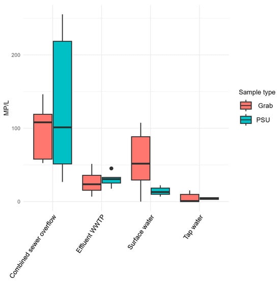
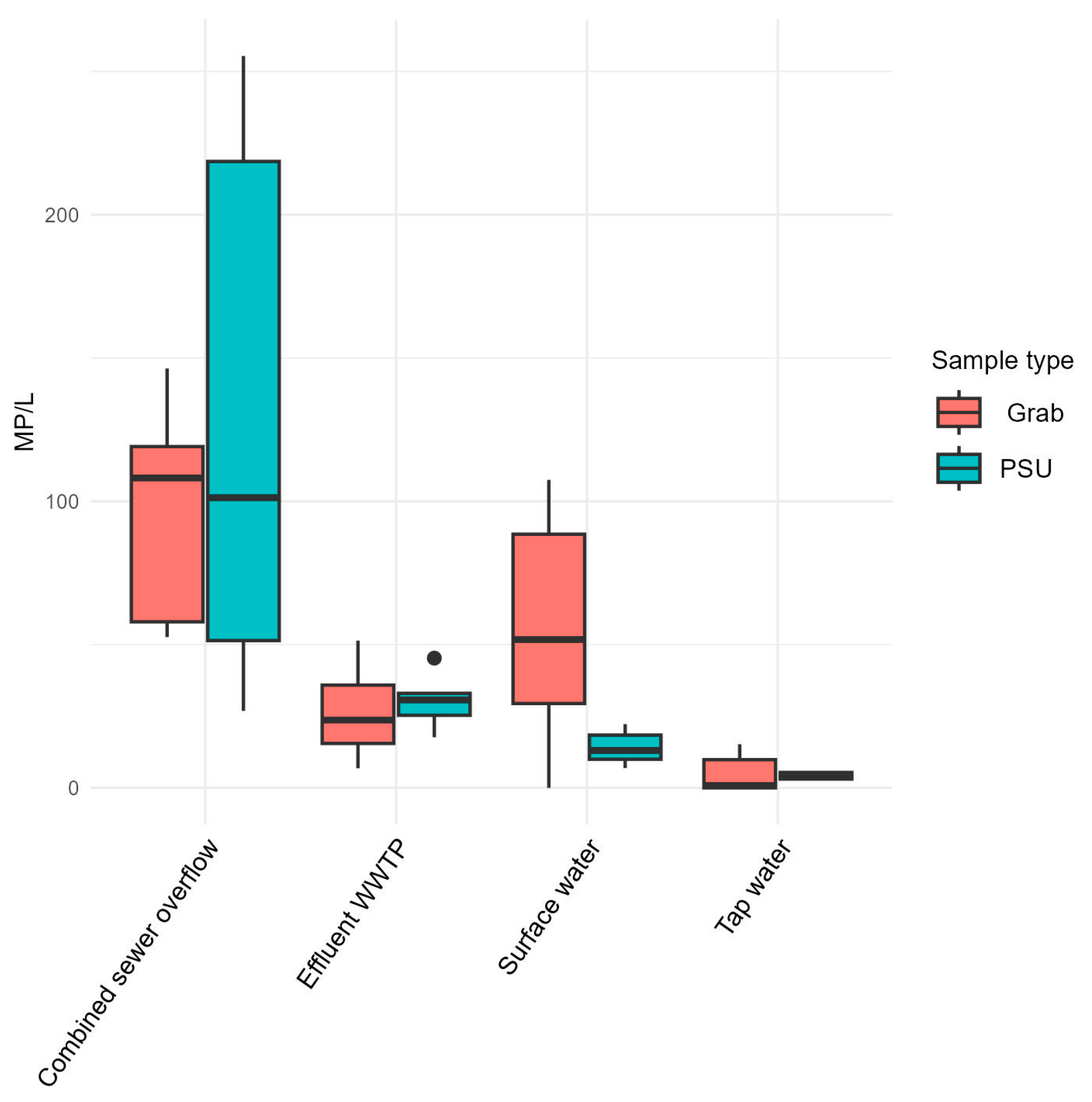
The standard deviation (S.D.) captures variability across the five replicates (grab samples) or five subsamples (PSU), while the relative standard deviation (R.S.D.) expresses this as a percentage of the mean, enabling precision comparisons across datasets of differing MP concentrations. To evaluate the effect of the sample volume, small-volume grab samples (0.5 L, analyzed in full) are compared with large-volume PSU samples (100 L, subsampled prior to analysis) using unspiked samples (Figure 4, Table 3).
Figure 4.
Comparison of detected MP/L of grab and PSU samples without spiking.
Table 3.
MP concentrations per sample for the different sample locations, sample types, and spiking conditions.
Grab samples show an absolute S.D. ranging from 7.7 MP/L for TW to 38.9 MP/L for SW. Comparing the R.S.D. values, the TW samples have the highest R.S.D., with 90%, and the CSO has the lowest, with 37%. As the TW samples have the lowest levels of MP contamination, they are more susceptible to measurement fluctuations due to background contamination or blank contamination. At higher concentrations, background contamination plays a smaller role, and the uneven distribution of MPs within the samples mainly influences the variance. For TW samples, an average of 8.6 MP/L was detected. In comparison, CSO samples had an average of 96.8 MP/L. Because no sampling or field blanks were included, the number of MPs detected in the TW samples may be overestimated. As TW had the lowest MP contamination, it was expected to be impacted the most by possible contamination during sampling.
For the PSU samples, the S.D. ranges from 1 MP/L for TW to 90.8 MP/L for CSO samples. The TW samples have the lowest R.S.D., with 25%, and CSO has the highest R.S.D., with 70%. Because the S.D. reflects the variability among the five subsamples taken from the same sample bottle, it results from the uneven distribution of MPs during subsampling. In addition, analyzing only part of the filter represents another subsampling step, which can introduce further variability, as particles are not evenly distributed across the filter surface. Scanning of the five squares of the filter covers 7% of the filter’s total surface. Regarding the high R.S.D. of the CSO, one possible explanation is that the heterogeneity of the particles in the CSO sample leads to a more irregular distribution compared to the other samples. Confirmation of this hypothesis would require further investigation, e.g., polymer-specific analysis or examination of particle sizes and shapes.
Comparing the R.S.D. values from the grab and PSU samples directly, the grab samples show an average R.S.D. of 64 ± 19%, while the PSU samples show a lower R.S.D of 41 ± 17%. For three of the four sampling locations (WWTP, SW, and TW), the PSU samples have a lower S.D. (Figure 5). Thus, despite the subsampling and partial analysis of the filter, the larger sampling volume of the PSU leads to higher precision compared to the 0.5 L grab samples for these applications.
Figure 5.
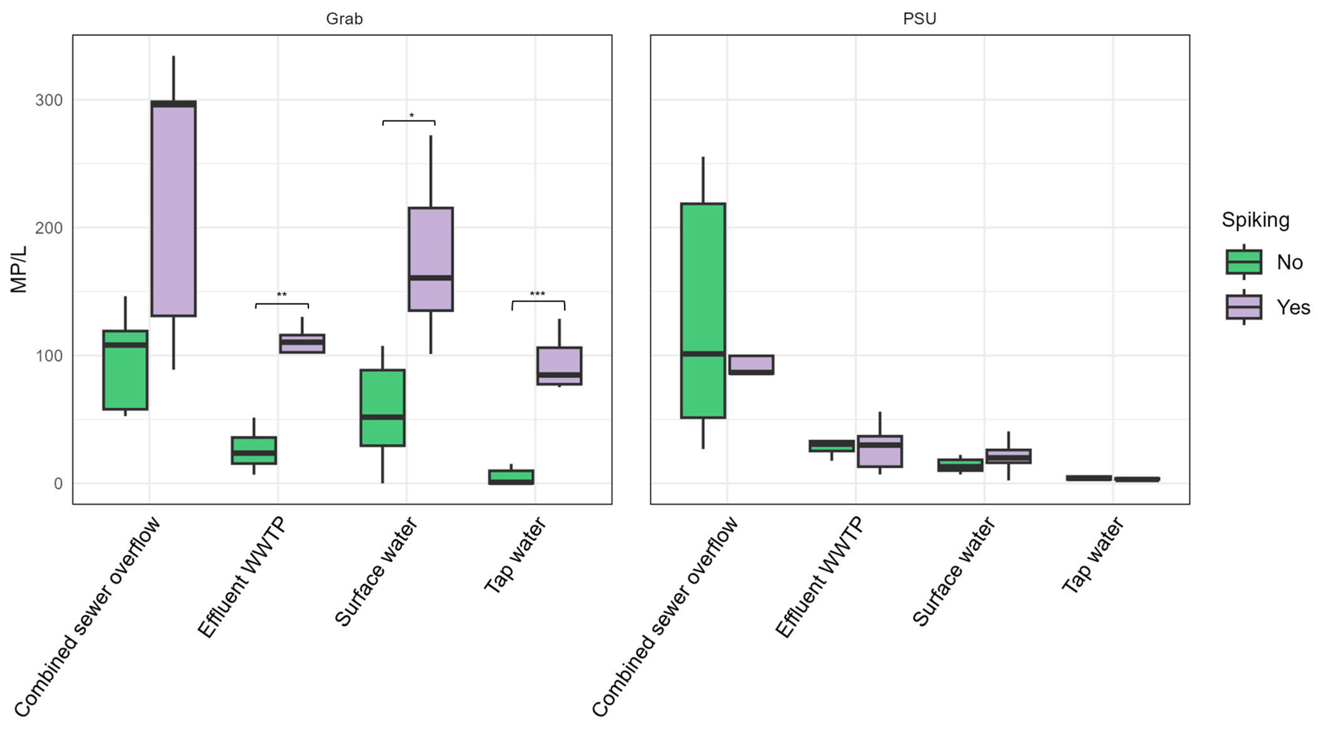
Comparison of detected MP/L for spiked and non-spiked samples. * = p < 0.05, ** = p < 0.01, *** = p < 0.001 (unpaired, two-sided Welch’s t-test).
Only CSO samples show a lower S.D. among the grab samples. This may be influenced by the IBC-based sampling procedure as an additional subsampling step (compared in the discussion in Section 3.3). The water in the IBC is mixed by a stirrer; subsequently, the PSU and grab samples were taken. Here, the additional subsampling and partial analysis of the filter surface for the PSU samples seems to have introduced higher uncertainties than the full sample processing and analysis from the grab samples, despite their lower volumes.
Comparing these results to those of other studies, in general, larger sample volumes were found to be more reliable for waters with low MP contamination, while small sample volumes are suitable for highly contaminated waters [15,44,45]. In addition, small sample volumes result in higher variability between replicates [44]. Cross et al. (2025) found a negative correlation between the sample volume and detected MPs and therefore recommend higher sample volumes for representative sampling [46]. However, this trend could not be observed in the current study, as there were no statistically significant differences between grab and PSU samples when comparing the levels of MP pollution at the respective sampling locations.
Subsampling, as conducted in the PSU samples, can introduce additional uncertainty and variability because MP particles are not evenly distributed within each sample, and every additional processing step increases the risk of error [47,48,49]. Despite these drawbacks, subsampling can significantly reduce the time and cost of analysis. Subsampling can involve taking only a portion of the original MP sample or analyzing only part of the material, such as examining a limited number of squares on a filter. In cases where particle loads are extremely high, subsampling may even be necessary to make the analysis more manageable [49]. Feng et al. (2025) reported that random grid subsampling of a 4–8% area resulted in 8–17% errors regarding particle numbers [48].
Furthermore, an interlaboratory study by Ciornii et al. (2025) among 56 laboratories worldwide, comparing the recovery of spiked pure water samples, found overall average R.S.D. values of 14–28% for µFTIR, 12–40% for µRaman, and 14–28% for GC-MS-based methods [50].
3.2. Spiking Experiments
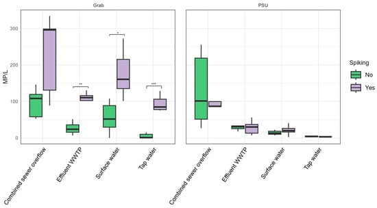
For the 0.5 L grab samples, the total difference between spiked and unspiked samples ranges from 76 ± 14 MP/L for WWTP samples to 133 ± 47 MP/L for CSO samples (Figure 5, Table 2). These deviate from the expected difference of 100 MP/L, due to the spiking with 50 MPs, by -24 MP for WWTP and +33 MP for CSO samples.
This corresponds to relative accuracy for spiking of 76% (WWTP) and 133% (CSO), respectively, indicating over- and underestimations. The SW samples show values within 121 ± 32, indicating a similar range to the CSO samples. The TW samples, which have the lowest background contamination with MPs, reach 91 ± 10 MP/L, with 91% relative accuracy for targeted spiking.
For the PSU samples, the 250 spiked particles were distributed in one of the 2.5 L sample bottles derived from the 100 L sample, resulting in targeted spiking of 2.5 MP/L. PSU samples exhibited substantial deviations, with differences ranging from −23.5 ± 49.5 MP/L (CSO) to 6.9 ± 6.1 MP/L (SW). Compared to the grab samples, the PSU samples had a higher total particle load (e.g., >2000 MP/L in the CSO) due to the large sample volume. Thus, the added particles represent only a small fraction of the total MP content in each of the five PSU subsamples. Therefore, measurement fluctuations (as discussed in Section 3.1) mask the spiking effect. In contrast, grab samples contain fewer background particles and a higher relative spike concentration (100 MP/L), resulting in a more pronounced spiking effect and more consistent recovery.
Accurate recovery can only be achieved if the spiked MPs exceed the fluctuations of the particles in the samples or if a large number of samples provides a close approximation of the true mean value, compensating for the large measurement fluctuations. Grab sampling showed greater accuracy because the spiked particles accounted for a much higher proportion of the total particles per sample than in the PSU.
Lares et al. (2019) conducted spiking experiments on wastewater, adding 70 MP particles to 0.1–1 L of wastewater. The reported recovery rates were 91.4% and 92.9%, and this strategy was found to be helpful to evaluate the accuracy of the detection method [51]. Hampton et al. (2023) conducted spiking experiments in different environmental matrices and found 60–70% recovery for particles >212 μm but 2% recovery for particles <20 μm [52]. Furthermore, the more complex the matrix was, the lower the recovery due to the additional processing steps. Extraction from sediment was the most problematic.
Another important factor to consider regarding accurate results is the risk of false positives caused by natural particles that can be mistakenly identified as MPs. A previous study that developed the method used here for sample processing and fluorescence staining-based detection also evaluated the risk of false positive results [43]. After hydrogen peroxide treatment (1 h at 100 °C) and fluorescence-based detection, the false positive rate ranged from 6% for chitin to 5% for chalk and wood.
Furthermore, the fluorescent staining method used in this study can only distinguish MPs based on a brightness threshold applied to the fluorescence images [43]. As a result, the method allows the quantification of MP particles in the sample, but it does not enable the identification of the polymer types. Recent research shows that polymer differentiation may become possible through AI-based analysis of solvatochromic shifts in fluorescent dyes or through fluorescence lifetime imaging approaches [36,53].
3.3. Recovery Rates
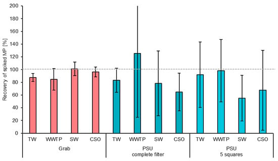
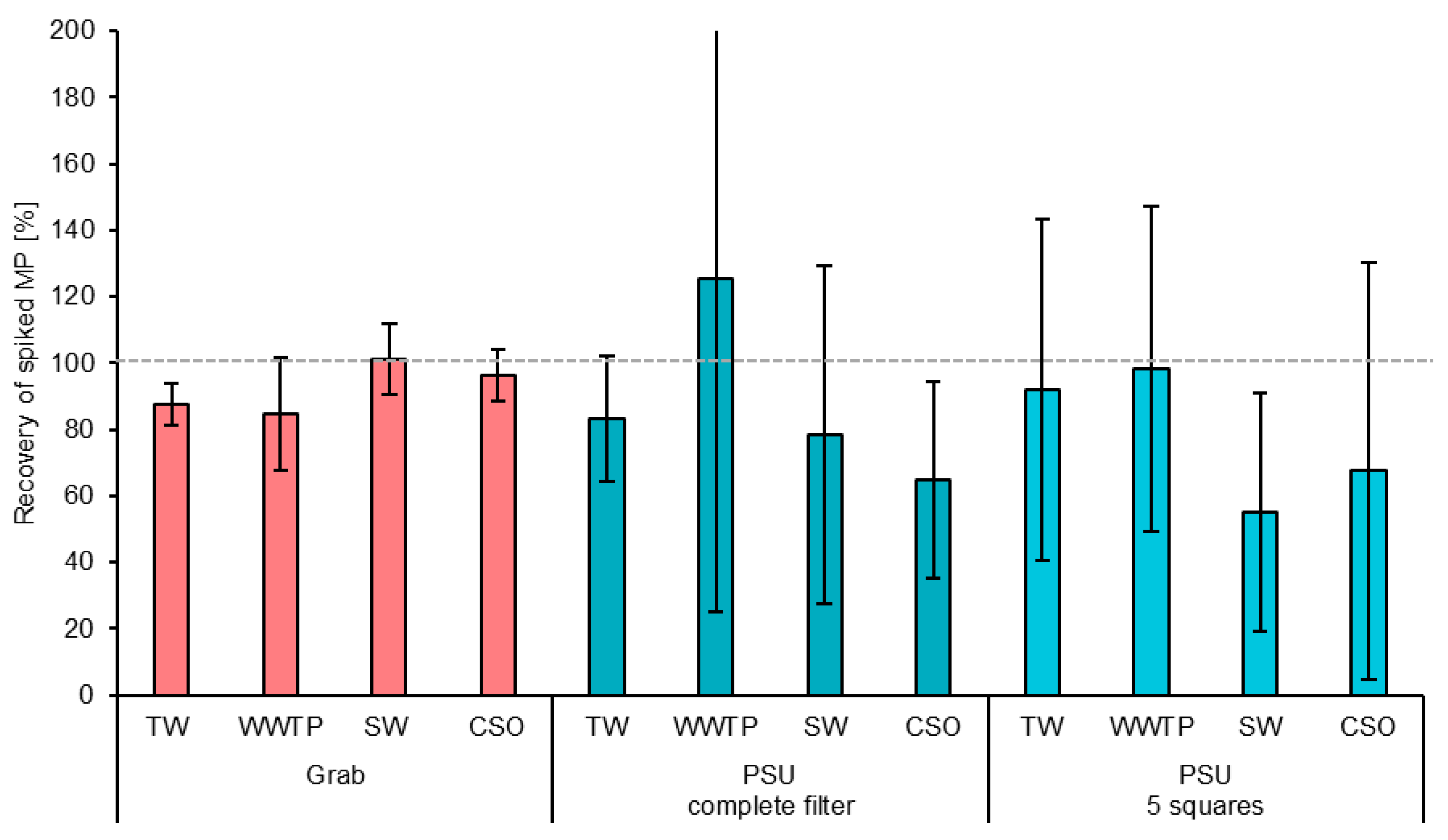
Recovery rates were calculated through the optical identification of the spiked PA particles based on their typical size, shape, and color. Grab samples with the complete filter analyzed were compared to PSU samples, whereby five squares of the filter were analyzed in addition to the complete filter (Figure 6).
Figure 6.
Recovery rates of spiked PA particles in different samples. Recovered PA was detected by optical identification of PA particles by their typical shape, size, and color.
The grab samples showed average recovery of 93 ± 7%, followed by the PSU samples with the complete filter analyzed, with 88 ± 23%. The lowest recovery was found for the PSU samples with five squares, with 78 ± 18%. The five analyzed squares represented 7% of the total filter surface. Although no statistically significant differences were observed between the average recovery rates (t-test, two-sided, unpaired, p > 0.05), subsampling only five squares appears to lead to the underestimation of MP contamination. This is most likely because more particles tended to accumulate at the contact area between the black filter membrane and the funnel during the final vacuum filtration of the processed and stained samples. These edge areas are not representatively covered by the five squares.
The MPs used in this study, with an average size of 357 µm, remained visible to the naked eye, which reduced the likelihood of particle loss during sample processing and transfer. It is well established that recovery rates decline for smaller MPs that can no longer be visually detected [20].
A previous study evaluating the recovery performance of the sample processing and detection method presented here reported recovery rates between 93.3% (polypropylene) and 101.7% (polyester) for industrial polymer granulates composed of polyethylene, polypropylene, polyamide, polyvinyl chloride, and polyester [43]. However, it should be noted that hydrogen peroxide digestion at 100 °C may degrade certain types of microplastics. Very small particles and polymers that are sensitive to heat or oxidation, as well as aged or environmentally transformed MPs, may be more susceptible to degradation under these conditions [54].
To assess the distribution of the spiked MPs across the five samples and subsamples at each location, the S.D. of each sampling was first calculated (see error bars in Figure 4); subsequently, the average of these S.D. values was calculated. The grab samples showed a lower average S.D. of 11% compared to the PSU samples, with an average S.D. of 50% for both complete and partial filter analysis. This suggests that measuring five squares reduces accuracy, reflected in the lower mean recovery, but does not reduce the precision, which is reflected in the S.D. values. The higher variability in the PSU samples compared to the grab samples is likely due to the additional subsampling step, during which MPs were unevenly distributed across the five subsamples.
The comparison with the R.S.D. values of the detected MPs in unspiked grab samples and PSU samples (Section 3.1) shows higher precision for the PSU samples, reflected in their lower overall R.S.D. values. This difference can be attributed to the source of variability in each sampling approach. MPs are highly heterogeneously distributed in aquatic environments. For grab samples, the variability is mainly driven by natural fluctuations in MP concentrations in the water, caught in the five subsequent samples. In contrast, PSU samples combine all subsamples from a single collected sample, so their variability is introduced solely through the subsampling process. Consequently, the variability between the five grab samples exceeds the variability caused by subsampling in the PSU samples.
An exception occurred in the CSO samples, where PSU samples showed a greater R.S.D. than grab samples. This can be explained by the sampling setup: the CSO water was collected in a single large IBC container. In this situation, the grab samples effectively functioned as subsamples of the same container, making them more similar to the PSU subsamples.
Way et al. (2022) conducted a meta-analysis of recovery rate studies and found that the recovery rates varied substantially depending on the sample matrix and extraction methodology [19]. Their analysis revealed that the recovery rates were the highest for plant material, whole organisms, and excrement (>88%), while significantly lower rates were observed for fishmeal, water, and soil matrices (58–71%). Critically, their findings suggest overall underestimation of MP concentrations of approximately 14% across the studies reviewed. Dimante-Deimantovica et al. (2022) demonstrated that 100 µm particles exhibited recovery rates ranging between 40% and 80%, declining further with increasing numbers of transfer steps during sample preparation [55].
Interlaboratory comparison exercises have proven essential in assessing the state of the art in MP detection and quantification methods. Isobe et al. (2019) conducted an interlaboratory comparison across 12 experienced laboratories worldwide using standardized seawater samples containing known quantities of MPs [56]. Their results revealed that MPs < 1 mm were underestimated by approximately 20%, even when using best practices. Van Mourik et al. (2021) reported the first global interlaboratory study on MPs under the WEPAL-QUASIMEME/NORMAN framework, finding that the analysis of particle numbers in soda tablets varied considerably between laboratories (29–91% recovery) [57]. These findings highlight the complexity of MP analysis and the urgent need for the harmonization of both reporting formats and analytical methods.
El Khatib et al. (2023) systematically investigated filter subsampling methods for Raman-based spectroscopic analysis and determined that analyzing a 12.5% fraction of the filter in a wedge shape provides an appropriate representation of the entire filter while substantially reducing the analysis time [58]. However, Brandt et al. (2021) demonstrated, through an assessment of various subsampling strategies, that a maximum subsampling error of 20% requires the analysis of either 50% of all particles or a minimum of 7000 particles in total [47]. Their findings further emphasize the critical importance of effective sample purification measures to increase the MP fraction, which not only shortens the analysis time but also improves the reliability of extrapolation when applying subsampling methods.
The development of reference materials represents another crucial step toward method standardization. Martinez-Frances et al. (2023) presented innovative reference materials for method validation in MP analysis, including dissolvable soda capsules and soda tablets containing known quantities of MP particles [59]. Their approach demonstrated that soda tablets and capsules containing MPs > 50 µm could be produced with sufficient precision (relative standard deviation 8–21%) for internal recovery tests and external interlaboratory comparison studies. More recently, Badzoka et al. (2025) introduced a novel method utilizing potassium bromide pellets embedded with MPs for precise particle count determination, achieving recovery rates above 95% for different polymer types, including LDPE, PVC, and polystyrene beads [40].
3.4. Confidence Interval and Beta Error
In this section, we discuss how the measured S.D. can be used to obtain insights into the precision of measurements and measurement campaigns. For simplification, the average R.S.D. values across all four sampling locations for grab and PSU samples from Section 3.1 are considered. All variables and assumptions are listed in Table 4.
Table 4.
Assumptions for the calculation of the margin of error of the C.I. for multiple sampling with PSU and grab samples.
The confidence interval (C.I.) is a range of values, derived from sample data, that is likely to contain the true mean value with a specified probability, called the confidence level. Under these assumptions, this means that, with 95% confidence (α = 5%) and in 8 out of 10 experiments (β = 20%), the true mean lies within the calculated margin of error.
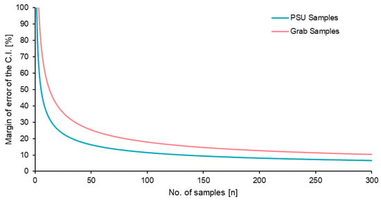
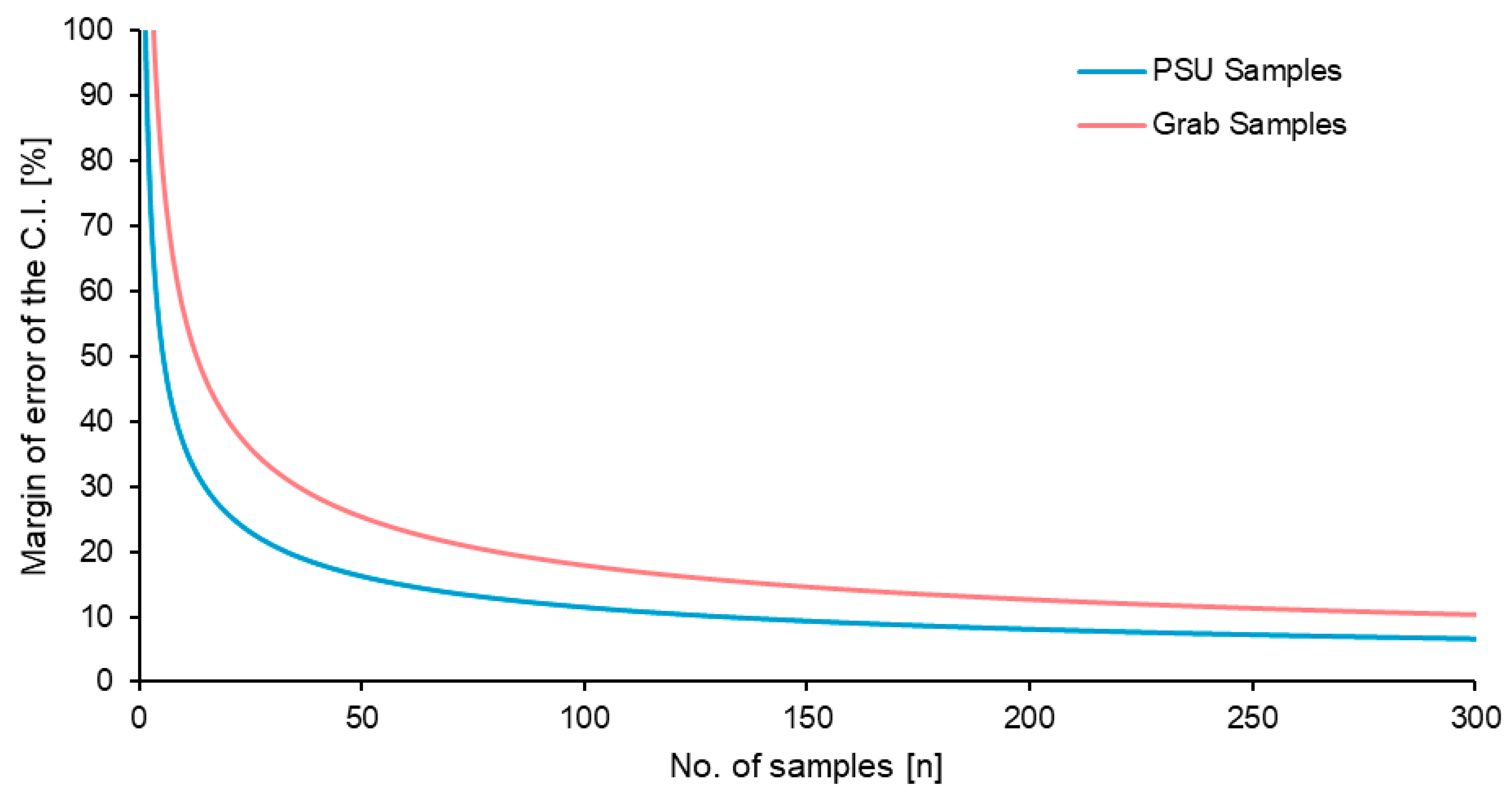
For five samples, as used in this study, a margin of error for the PSU of ±51% was found; for grab sampling, this was ±80% (Figure 7). To reach a margin of error of 25%, for the PSU, 21 samples would be needed, while 51 grab samples would be required. A 10% margin of error would need 131 PSU and 312 grab samples. These values further demonstrate the challenges of monitoring MPs in aquatic environments, where their heterogeneous distributions lead to substantial variability. They also underline that multiple measurements are essential to obtain reliable and accurate results.
Figure 7.
Margin of error for the confidence interval (C.I.) calculated for the number of sample replicates (n). Assumptions for the calculations are listed in Table 3.
It is noteworthy that the relationship between the R.S.D. or S.D. and the number of samples required to achieve a given margin of error is quadratic. As a result, halving the standard deviation reduces the required sample size to one quarter. This means that even small improvements in the measurement procedure that reduce measurement variability can substantially increase the precision of the results.
PSU samples generally provide higher precision, making them more suitable for obtaining accurate single-point measurements. In contrast, grab samples are easier to collect but less precise. Their reduced accuracy can be compensated for by increasing the number of samples taken, thereby improving overall reliability.
A literature review by Greenshields et al. (2024) found that only one replicate was used in 62% of studies, and they recommended that a minimum of three replicates should be used over the area of interest [60]. She at al. (2022) demonstrated that trawl datasets exhibited spatiotemporal sampling errors of approximately 25% for microlitter concentrations, 36% for MP fiber concentrations, and 40–56% for MP particle concentrations [61].
Lyykemark et al. (2025) conducted Monte Carlo simulations on an MP dataset from marine sediments [62]. Their analysis showed that, with only 10 sampling points, there is a 50% probability that the sample mean will fall within 94–119% of the true mean, defined as the overall mean in their study. Klemmensen et al. (2024) used Monte Carlo simulations to show that relying on a single soil sample can lead to substantial errors [63]. In their analysis, 50% of single-sample measurements deviated by as much as 70% from the true mean particle concentration. With ten sampling points, the deviation decreased to 26%, and, with 20 sampling points, it was further reduced to 14%. These results highlight the need for sufficiently large sample numbers to reliably characterize MP pollution.
4. Conclusions
The comparison of grab samples (0.5 L) and PSU samples (100 L) revealed substantial differences in measurement precision across all sampling locations. Despite the additional variability introduced by the subsampling procedures, PSU sampling demonstrated superior precision compared to conventional grab sampling. The mean relative standard deviation (R.S.D.) for grab samples was 64 ± 19%, whereas PSU samples exhibited a significantly lower R.S.D. of 41 ± 17%. This finding was consistent across three of the four sampling locations (WWTP, SW, and TW), with the exception of CSO samples, where the PSU variability exceeded that of grab sampling, most likely due to the specific sampling protocol employed.
The enhanced precision of PSU sampling can be attributed to the larger sample volume, which effectively captures a more representative fraction of the heterogeneously distributed MP particles in the water column. The natural fluctuation in MP concentrations between individual grab samples exceeded the variability introduced by the PSU subsampling process, indicating that spatial heterogeneity in aquatic environments represents the dominant source of measurement uncertainty in MP monitoring.
In MP recovery, grab sampling showed substantially higher accuracy than PSU sampling. Grab sampling with complete filter analysis achieved the highest mean recovery of 93 ± 7%. PSU sampling with complete filter analysis showed comparable performance (88 ± 23%), while partial filter analysis (five discrete tiles representing 7% of the filter surface) resulted in reduced recovery (78 ± 18%). In grab samples, spiked particles represented a much larger proportion of the total particle load. These results highlight that reliable recovery is only achievable when the spiked MPs exceed the natural variability or when a sufficiently large number of samples is analyzed.
Notably, while partial filter analysis decreased accuracy (as reflected in the lower mean recovery), it did not significantly affect the precision, as evidenced by the comparable standard deviations for complete filter analysis. This observation suggests that the tile-based scanning approach introduces systematic underestimation rather than random errors, which may be addressed through appropriate correction factors in routine monitoring applications.
Based on the measured R.S.D. values, the number of samples required to achieve defined margins of error was calculated using beta statistics (α = 0.05, β = 0.2). For the five replicate samples employed in this study, the margin of error at 95% confidence was ±51% for PSU samples and ±80% for grab samples.
The quadratic relationship between the standard deviation and required sample number has important practical implications. Consequently, methodological improvements that reduce analytical variability, such as optimized subsampling procedures, enhanced homogenization protocols, or increased filter coverage during microscopic analysis, can substantially improve the cost-effectiveness of MP monitoring programs.
In conclusion, PSU sampling provides higher precision for single-point measurements, making it more suitable for applications requiring accurate concentration estimates from limited sampling events. Grab sampling, while less precise, offers practical advantages in terms of ease of collection and can achieve comparable accuracy through increased replication. Thus, grab sampling is preferable if a high number of samples is needed or if the application of a PSU is impractical. The choice between methods should be guided by the specific objectives of the monitoring program, the available resources, and the acceptable margin of error for the intended application.
Author Contributions
Conceptualization, M.T.S., M.W., and K.S.; methodology, M.T.S. and K.S.; validation, M.T.S. and K.S.; formal analysis, A.K., M.T.S., and K.S.; investigation, M.W., P.R., and M.T.S.; resources, K.S.; data curation, M.T.S., E.M., and K.S.; writing—original draft preparation, M.T.S., E.M., and K.S.; writing—review and editing, A.K., M.T.S., E.M., and K.S.; visualization, E.M. and M.T.S.; supervision, K.S.; project administration, K.S.; funding acquisition, K.S. All authors have read and agreed to the published version of the manuscript.
Funding
The authors gratefully acknowledge the financial support of the Horizon Mission project UPSTREAM (GA 101112877), co-funded by the European Union and UK Research and Innovation. This publication reflects the views only of the authors, and the European Commission cannot be held responsible for any use that may be made of the information contained herein. The project also received part of its funding from the Veolia Foundation (Germany) project konti|detect.
Data Availability Statement
Full data are available on reasonable request from the corresponding author.
Acknowledgments
The authors thank Entsorgungs und Wirtschaftsbetriebe Landau (EWL, Germany) and abcr GmbH Karlsruhe for the project-related support.
Conflicts of Interest
The authors Michael Toni Sturm, Pieter Ronsse, Erika Myers, and Katrin Schuhen were employed by the company Wasser 3.0 gGmbH. Mirjam Wielandt was an intern for a 10-week period at Wasser 3.0 gGmbH. She supported the research work as part of her training at Heinrich-Lanz-Schule, Mannheim, Germany. All authors declare that the research was conducted in the absence of any commercial or financial relationships that could be construed as a potential conflict of interest.
Abbreviations
The following abbreviations are used in this manuscript:
| CSO | Combined sewer overflow |
| FTIR | Fourier-transform infrared |
| m% | Margin of error in percent |
| MP | Microplastic |
| PA | Polyamide |
| PE | Population equivalents |
| PSU | Particle sampling unit |
| QA | Quality assurance |
| QC | Quality control |
| R.S.D. | Relative standard deviation |
| S.D. | Standard deviation |
| SW | Surface water |
| TSS | Total suspended solids |
| TW | Tap water |
| WWTP | Wastewater treatment plant |
References
- Pulusu, V.S.; Chilamula, S.; Holkunde, A.; Gunturi, R.; Vidiyala, P.; Bashetty, S.R. Microplastics and Nanoplastics: Environmental Pathways, Ecological Impacts, and Regulatory Perspectives. Open Access Libr. J. 2025, 12, e13696. [Google Scholar] [CrossRef]
- Horton, A.A.; Walton, A.; Spurgeon, D.J.; Lahive, E.; Svendsen, C. Microplastics in freshwater and terrestrial environments: Evaluating the current understanding to identify the knowledge gaps and future research priorities. Sci. Total Environ. 2017, 586, 127–141. [Google Scholar] [CrossRef] [Scilit]
- Thompson, R.C.; Courtene-Jones, W.; Boucher, J.; Pahl, S.; Raubenheimer, K.; Koelmans, A.A. Twenty years of microplastic pollution research-what have we learned? Science 2024, 386, eadl2746. [Google Scholar] [CrossRef] [Scilit]
- Wagner, M.; Scherer, C.; Alvarez-Muñoz, D.; Brennholt, N.; Bourrain, X.; Buchinger, S.; Fries, E.; Grosbois, C.; Klasmeier, J.; Marti, T.; et al. Microplastics in freshwater ecosystems: What we know and what we need to know. Environ. Sci. Eur. 2014, 26, 12. [Google Scholar] [CrossRef] [Scilit]
- Zhang, K.; Hamidian, A.H.; Tubić, A.; Zhang, Y.; Fang, J.K.H.; Wu, C.; Lam, P.K.S. Understanding plastic degradation and microplastic formation in the environment: A review. Environ. Pollut. 2021, 274, 116554. [Google Scholar] [CrossRef] [Scilit]
- Yousafzai, S.; Farid, M.; Zubair, M.; Naeem, N.; Zafar, W.; Zaman Asam, Z.U.; Farid, S.; Ali, S. Detection and degradation of microplastics in the environment: A review. Environ. Sci. Adv. 2025, 4, 1142–1165. [Google Scholar] [CrossRef] [Scilit]
- Bhowmik, A.; Saha, G. Microplastics in Our Waters: Insights from a Configurative Systematic Review of Water Bodies and Drinking Water Sources. Microplastics 2025, 4, 24. [Google Scholar] [CrossRef] [Scilit]
- Thompson, R.C.; Olsen, Y.; Mitchell, R.P.; Davis, A.; Rowland, S.J.; John, A.W.G.; McGonigle, D.; Russell, A.E. Lost at sea: Where is all the plastic? Science 2004, 304, 838. [Google Scholar] [CrossRef] [Scilit] [PubMed]
- Hidalgo-Ruz, V.; Gutow, L.; Thompson, R.C.; Thiel, M. Microplastics in the marine environment: A review of the methods used for identification and quantification. Environ. Sci. Technol. 2012, 46, 3060–3075. [Google Scholar] [CrossRef] [Scilit] [PubMed]
- Koelmans, A.A.; Mohamed Nor, N.H.; Hermsen, E.; Kooi, M.; Mintenig, S.M.; de France, J. Microplastics in freshwaters and drinking water: Critical review and assessment of data quality. Water Res. 2019, 155, 410–422. [Google Scholar] [CrossRef] [Scilit] [PubMed]
- Hermsen, E.; Mintenig, S.M.; Besseling, E.; Koelmans, A.A. Quality Criteria for the Analysis of Microplastic in Biota Samples: A Critical Review. Environ. Sci. Technol. 2018, 52, 10230–10240. [Google Scholar] [CrossRef] [Scilit]
- Singh, B.; Kumar, A. Advances in microplastics detection: A comprehensive review of methodologies and their effectiveness. TrAC Trends Anal. Chem. 2024, 170, 117440. [Google Scholar] [CrossRef] [Scilit]
- Löder, M.G.J.; Gerdts, G. Methodology Used for the Detection and Identification of Microplastics—A Critical Appraisal. In Marine Anthropogenic Litter; Bergmann, M., Gutow, L., Klages, M., Eds.; Springer International Publishing: Cham, Switzerland, 2015; pp. 201–227. ISBN 978-3-319-16509-7. [Google Scholar]
- Cai, M.; Liu, M.; Hossain, K.B.; Wang, J.; Zhou, Y.; Yan, M.; Leung, K.M. Current status and emerging techniques for sampling, separating, and identifying microplastics in freshwater environments. TrAC Trends Anal. Chem. 2025, 184, 118151. [Google Scholar] [CrossRef] [Scilit]
- Prata, J.C.; Da Costa, J.P.; Duarte, A.C.; Rocha-Santos, T. Methods for sampling and detection of microplastics in water and sediment: A critical review. TrAC Trends Anal. Chem. 2019, 110, 150–159. [Google Scholar] [CrossRef] [Scilit]
- Razeghi, N.; Hamidian, A.H.; Mirzajani, A.; Abbasi, S.; Wu, C.; Zhang, Y.; Yang, M. Sample preparation methods for the analysis of microplastics in freshwater ecosystems: A review. Environ. Chem. Lett. 2022, 20, 417–443. [Google Scholar] [CrossRef] [Scilit]
- de Ruijter, V.N.; Redondo-Hasselerharm, P.E.; Gouin, T.; Koelmans, A.A. Quality Criteria for Microplastic Effect Studies in the Context of Risk Assessment: A Critical Review. Environ. Sci. Technol. 2020, 54, 11692–11705. [Google Scholar] [CrossRef] [Scilit] [PubMed]
- Shao, K.; Zou, R.; Zhang, Z.; Mandemaker, L.D.B.; Timbie, S.; Smith, R.D.; Durkin, A.M.; Dusza, H.M.; Meirer, F.; Weckhuysen, B.M.; et al. Advancements in Assays for Micro- and Nanoplastic Detection: Paving the Way for Biomonitoring and Exposomics Studies. Annu. Rev. Pharmacol. Toxicol. 2025, 65, 567–585. [Google Scholar] [CrossRef] [Scilit]
- Way, C.; Hudson, M.D.; Williams, I.D.; Langley, G.J. Evidence of underestimation in microplastic research: A meta-analysis of recovery rate studies. Sci. Total Environ. 2022, 805, 150227. [Google Scholar] [CrossRef] [Scilit] [PubMed]
- Weber, F.; Kerpen, J. Underestimating microplastics? Quantification of the recovery rate of microplastic particles including sampling, sample preparation, subsampling, and detection using µ-Ramanspectroscopy. Anal. Bioanal. Chem. 2023, 415, 2963–2973. [Google Scholar] [CrossRef] [Scilit] [PubMed]
- de Frond, H.; O’Brien, A.M.; Rochman, C.M. Representative subsampling methods for the chemical identification of microplastic particles in environmental samples. Chemosphere 2023, 310, 136772. [Google Scholar] [CrossRef] [Scilit]
- Munno, K.; Lusher, A.L.; Minor, E.C.; Gray, A.; Ho, K.; Hankett, J.; Lee, C.-F.T.; Primpke, S.; McNeish, R.E.; Wong, C.S.; et al. Patterns of microparticles in blank samples: A study to inform best practices for microplastic analysis. Chemosphere 2023, 333, 138883. [Google Scholar] [CrossRef] [Scilit] [PubMed]
- Brander, S.M.; Renick, V.C.; Foley, M.M.; Steele, C.; Woo, M.; Lusher, A.; Carr, S.; Helm, P.; Box, C.; Cherniak, S.; et al. Sampling and Quality Assurance and Quality Control: A Guide for Scientists Investigating the Occurrence of Microplastics Across Matrices. Appl. Spectrosc. 2020, 74, 1099–1125. [Google Scholar] [CrossRef] [Scilit] [PubMed]
- Xu, J.-L.; Thomas, K.V.; Luo, Z.; Gowen, A.A. FTIR and Raman imaging for microplastics analysis: State of the art, challenges and prospects. TrAC Trends Anal. Chem. 2019, 119, 115629. [Google Scholar] [CrossRef] [Scilit]
- Araujo, C.F.; Nolasco, M.M.; Ribeiro, A.M.P.; Ribeiro-Claro, P.J.A. Identification of microplastics using Raman spectroscopy: Latest developments and future prospects. Water Res. 2018, 142, 426–440. [Google Scholar] [CrossRef] [Scilit]
- Primpke, S.; Lorenz, C.; Rascher-Friesenhausen, R.; Gerdts, G. An automated approach for microplastics analysis using focal plane array (FPA) FTIR microscopy and image analysis. Anal. Methods 2017, 9, 1499–1511. [Google Scholar] [CrossRef] [Scilit]
- Käppler, A.; Fischer, D.; Oberbeckmann, S.; Schernewski, G.; Labrenz, M.; Eichhorn, K.-J.; Voit, B. Analysis of environmental microplastics by vibrational microspectroscopy: FTIR, Raman or both? Anal. Bioanal. Chem. 2016, 408, 8377–8391. [Google Scholar] [CrossRef] [Scilit]
- Cabernard, L.; Roscher, L.; Lorenz, C.; Gerdts, G.; Primpke, S. Comparison of Raman and Fourier Transform Infrared Spectroscopy for the Quantification of Microplastics in the Aquatic Environment. Environ. Sci. Technol. 2018, 52, 13279–13288. [Google Scholar] [CrossRef] [Scilit]
- Fischer, M.; Scholz-Böttcher, B.M. Simultaneous Trace Identification and Quantification of Common Types of Microplastics in Environmental Samples by Pyrolysis-Gas Chromatography-Mass Spectrometry. Environ. Sci. Technol. 2017, 51, 5052–5060. [Google Scholar] [CrossRef] [Scilit]
- Hermabessiere, L.; Himber, C.; Boricaud, B.; Kazour, M.; Amara, R.; Cassone, A.-L.; Laurentie, M.; Paul-Pont, I.; Soudant, P.; Dehaut, A.; et al. Optimization, performance, and application of a pyrolysis-GC/MS method for the identification of microplastics. Anal. Bioanal. Chem. 2018, 410, 6663–6676. [Google Scholar] [CrossRef] [Scilit]
- Primpke, S.; Fischer, M.; Lorenz, C.; Gerdts, G.; Scholz-Böttcher, B.M. Comparison of pyrolysis gas chromatography/mass spectrometry and hyperspectral FTIR imaging spectroscopy for the analysis of microplastics. Anal. Bioanal. Chem. 2020, 412, 8283–8298. [Google Scholar] [CrossRef] [Scilit]
- Käppler, A.; Fischer, M.; Scholz-Böttcher, B.M.; Oberbeckmann, S.; Labrenz, M.; Fischer, D.; Eichhorn, K.-J.; Voit, B. Comparison of μ-ATR-FTIR spectroscopy and py-GCMS as identification tools for microplastic particles and fibers isolated from river sediments. Anal. Bioanal. Chem. 2018, 410, 5313–5327. [Google Scholar] [CrossRef] [Scilit]
- Maes, T.; Jessop, R.; Wellner, N.; Haupt, K.; Mayes, A.G. A rapid-screening approach to detect and quantify microplastics based on fluorescent tagging with Nile Red. Sci. Rep. 2017, 7, 44501. [Google Scholar] [CrossRef] [Scilit]
- van den Akker, K.; Mandemaker, L.D.B.; Dorresteijn, J.M.; Amaral-Zettler, L.A.; Weckhuysen, B.M.; Meirer, F. Fluorescent nanoplastics: What steps are needed towards a representative toolkit? Micropl. Nanopl. 2025, 6, 4. [Google Scholar] [CrossRef] [Scilit] [PubMed]
- Erni-Cassola, G.; Gibson, M.I.; Thompson, R.C.; Christie-Oleza, J.A. Lost, but Found with Nile Red: A Novel Method for Detecting and Quantifying Small Microplastics (1 mm to 20 μm) in Environmental Samples. Environ. Sci. Technol. 2017, 51, 13641–13648. [Google Scholar] [CrossRef] [Scilit] [PubMed]
- Meyers, N.; Catarino, A.I.; Declercq, A.M.; Brenan, A.; Devriese, L.; Vandegehuchte, M.; de Witte, B.; Janssen, C.; Everaert, G. Microplastic detection and identification by Nile red staining: Towards a semi-automated, cost- and time-effective technique. Sci. Total Environ. 2022, 823, 153441. [Google Scholar] [CrossRef] [Scilit]
- Sturm, M.T.; Myers, E.; Schober, D.; Korzin, A.; Schuhen, K. Development of an Inexpensive and Comparable Microplastic Detection Method Using Fluorescent Staining with Novel Nile Red Derivatives. Analytica 2023, 4, 27–44. [Google Scholar] [CrossRef] [Scilit]
- Sturm, M.T.; Korzin, A.; Ronsse, P.; Myers, E.; Zernikel, O.; Schober, D.; Schuhen, K. Reliable River Microplastic Monitoring Using Innovative Fluorescence Dyes—A Case Study. Microplastics 2025, 4, 63. [Google Scholar] [CrossRef] [Scilit]
- Sturm, M.T.; Argyropoulou, D.; Myers, E.; Korzin, A.; Ronsse, P.; Zernikel, O.; Schober, D.; Schuhen, K. Comparative Long-Term Monitoring of Microplastics in the Effluent of Three Different Wastewater Treatment Plants with Two, Three, and Four Treatment Stages. Water 2025, 17, 711. [Google Scholar] [CrossRef] [Scilit]
- Badzoka, J.; Kappacher, C.; Lauß, J.; Obwaller, L.; Pavun, A.; Huck, C.W. Enabling analytical precision in microplastic analysis: Innovative solutions for precise method validation, evaluation and quality control. Micropl. Nanopl. 2025, 5, 2. [Google Scholar] [CrossRef] [Scilit]
- Sturm, M.T.; Myers, E.; Korzin, A.; Schober, D.; Schuhen, K. Long-Term Monitoring of Microplastics in a German Municipal Wastewater Treatment Plant. Microplastics 2024, 3, 492–502. [Google Scholar] [CrossRef] [Scilit]
- Sturm, M.T.; Horn, H.; Schuhen, K. The potential of fluorescent dyes-comparative study of Nile red and three derivatives for the detection of microplastics. Anal. Bioanal. Chem. 2021, 413, 1059–1071. [Google Scholar] [CrossRef] [Scilit]
- Sturm, M.T.; Myers, E.; Korzin, A.; Polierer, S.; Schober, D.; Schuhen, K. Fast Forward: Optimized Sample Preparation and Fluorescent Staining for Microplastic Detection. Microplastics 2023, 2, 334–349. [Google Scholar] [CrossRef] [Scilit]
- Rodríguez-Alegre, R.; Durán-Videra, S.; Carmona-Fernández, D.; Pérez Megías, L.; Andecochea Saiz, C.; You, X. Comparative Assessment of Protocols for Microplastic Quantification in Wastewater. Microplastics 2025, 4, 49. [Google Scholar] [CrossRef] [Scilit]
- Saikia, K.K.; Handique, S. A Global Comparative Study on Microplastics Sampling, Identification and Quantification Techniques in Freshwater Environment: A Review. Water Air Soil Pollut 2026, 237, 284. [Google Scholar] [CrossRef] [Scilit]
- Cross, R.K.; Roberts, S.L.; Jürgens, M.D.; Johnson, A.C.; Davis, C.W.; Gouin, T. Ensuring representative sample volume predictions in microplastic monitoring. Micropl. Nanopl. 2025, 5, 5. [Google Scholar] [CrossRef] [Scilit]
- Brandt, J.; Fischer, F.; Kanaki, E.; Enders, K.; Labrenz, M.; Fischer, D. Assessment of Subsampling Strategies in Microspectroscopy of Environmental Microplastic Samples. Front. Environ. Sci. 2021, 8, 579676. [Google Scholar] [CrossRef] [Scilit]
- Feng, X.; Manek, V.; Andrews, R.C.; Almuhtaram, H. Sub-sampling strategies for analysis of small (<20 µm) microplastics in water. Water Res. 2025, 283, 123846. [Google Scholar] [CrossRef] [Scilit]
- Cowger, W.; Markley, L.A.T.; Moore, S.; Gray, A.B.; Upadhyay, K.; Koelmans, A.A. How many microplastics do you need to (sub)sample? Ecotoxicol. Environ. Saf. 2024, 275, 116243. [Google Scholar] [CrossRef] [Scilit]
- Ciornii, D.; Hodoroaba, V.-D.; Benismail, N.; Maltseva, A.; Ferrer, J.F.; Wang, J.; Parra, R.; Jézéquel, R.; Receveur, J.; Gabriel, D.; et al. Interlaboratory Comparison Reveals State of the Art in Microplastic Detection and Quantification Methods. Anal. Chem. 2025, 97, 8719–8728. [Google Scholar] [CrossRef] [Scilit]
- Lares, M.; Ncibi, M.C.; Sillanpää, M.; Sillanpää, M. Intercomparison study on commonly used methods to determine microplastics in wastewater and sludge samples. Environ. Sci. Pollut. Res. Int. 2019, 26, 12109–12122. [Google Scholar] [CrossRef] [Scilit] [PubMed]
- Thornton Hampton, L.M.; de Frond, H.; Gesulga, K.; Kotar, S.; Lao, W.; Matuch, C.; Weisberg, S.B.; Wong, C.S.; Brander, S.; Christansen, S.; et al. The influence of complex matrices on method performance in extracting and monitoring for microplastics. Chemosphere 2023, 334, 138875. [Google Scholar] [CrossRef] [Scilit]
- Monteleone, A.; Schary, W.; Wenzel, F.; Langhals, H.; Dietrich, D.R. Label-free identification and differentiation of different microplastics using phasor analysis of fluorescence lifetime imaging microscopy (FLIM)-generated data. Chem. Biol. Interact. 2021, 342, 109466. [Google Scholar] [CrossRef] [Scilit]
- Prata, J.C.; Da Costa, J.P.; Girão, A.V.; Lopes, I.; Duarte, A.C.; Rocha-Santos, T. Identifying a quick and efficient method of removing organic matter without damaging microplastic samples. Sci. Total Environ. 2019, 686, 131–139. [Google Scholar] [CrossRef] [Scilit] [PubMed]
- Dimante-Deimantovica, I.; Suhareva, N.; Barone, M.; Putna-Nimane, I.; Aigars, J. Hide-and-seek: Threshold values and contribution towards better understanding of recovery rate in microplastic research. MethodsX 2022, 9, 101603. [Google Scholar] [CrossRef] [Scilit] [PubMed]
- Isobe, A.; Buenaventura, N.T.; Chastain, S.; Chavanich, S.; Cózar, A.; DeLorenzo, M.; Hagmann, P.; Hinata, H.; Kozlovskii, N.; Lusher, A.L.; et al. An interlaboratory comparison exercise for the determination of microplastics in standard sample bottles. Mar. Pollut. Bull. 2019, 146, 831–837. [Google Scholar] [CrossRef] [Scilit]
- van Mourik, L.M.; Crum, S.; Martinez-Frances, E.; van Bavel, B.; Leslie, H.A.; de Boer, J.; Cofino, W.P. Results of WEPAL-QUASIMEME/NORMANs first global interlaboratory study on microplastics reveal urgent need for harmonization. Sci. Total Environ. 2021, 772, 145071. [Google Scholar] [CrossRef] [Scilit] [PubMed]
- El Khatib, D.; Langknecht, T.D.; Cashman, M.A.; Reiss, M.; Somers, K.; Allen, H.; Ho, K.T.; Burgess, R.M. Assessment of filter subsampling and extrapolation for quantifying microplastics in environmental samples using Raman spectroscopy. Mar. Pollut. Bull. 2023, 192, 115073. [Google Scholar] [CrossRef] [Scilit]
- Martínez-Francés, E.; van Bavel, B.; Hurley, R.; Nizzetto, L.; Pakhomova, S.; Buenaventura, N.T.; Singdahl-Larsen, C.; Magni, M.-L.T.; Johansen, J.E.; Lusher, A. Innovative reference materials for method validation in microplastic analysis including interlaboratory comparison exercises. Anal. Bioanal. Chem. 2023, 415, 2907–2919. [Google Scholar] [CrossRef] [Scilit]
- Greenshields, J.; Anastasi, A.; Irving, A.D.; Capper, A. A systematic review to assess current surface water and sediment microplastic sampling practices in seagrass and mangrove ecosystems. Environ. Sci. Pollut. Res. Int. 2024, 31, 66615–66629. [Google Scholar] [CrossRef] [Scilit]
- She, J.; Buhhalko, N.; Lind, K.; Mishra, A.; Kikas, V.; Costa, E.; Gambardella, C.; Montarsolo, A.; Faimali, M.; Garaventa, F.; et al. Uncertainty and Consistency Assessment in Multiple Microplastic Observation Datasets in the Baltic Sea. Front. Mar. Sci. 2022, 9, 886357. [Google Scholar] [CrossRef] [Scilit]
- Lykkemark, J.; Simon-Sánchez, L.; Liu, F.; Vianello, A.; Chand, R.; Vollertsen, J.; Christensen, M.L.; Nielsen, A.H. How many samples do we need to be representative? Grid sampling in Danish waters for assessing the distribution of microplastics and tire wear particles in seabed sediments. Mar. Pollut. Bull. 2025, 223, 119044. [Google Scholar] [CrossRef] [Scilit] [PubMed]
- Klemmensen, N.D.R.; Chand, R.; Blanco, M.S.; Vollertsen, J. Microplastic abundance in sludge-treated fields: Variance and estimated half-life. Sci. Total Environ. 2024, 922, 171394. [Google Scholar] [CrossRef] [Scilit] [PubMed]

Disclaimer/Publisher’s Note: The statements, opinions and data contained in all publications are solely those of the individual author(s) and contributor(s) and not of MDPI and/or the editor(s). MDPI and/or the editor(s) disclaim responsibility for any injury to people or property resulting from any ideas, methods, instructions or products referred to in the content. |
© 2026 by the authors. Licensee MDPI, Basel, Switzerland. This article is an open access article distributed under the terms and conditions of the Creative Commons Attribution (CC BY) license.