Multi-Layer Network Optimization of Data Centers Siting and Capacity Development

Abstract

The rapid growth of artificial intelligence applications and digital ecosystems, especially in industry, has highlighted the need for proposing new data centers. Data center siting requires consideration of many different factors including power grid capacity, fiber network resources, and environmental and regional considerations. This research proposes a multi-layer network optimization in which the master plan optimizes data center siting and their capacity decisions while the other lower-level layers analyze the feasibility and optimality of these decisions in terms of grid congestion and transmission network expansion, fiber routing and latency, and cooling resources. The efficiency of the proposed plan and its reliability will be evaluated by simulating different scenarios including unexpected power grid outages because of natural disasters. The results of the model highlight the importance of integrated decision making for siting data centers while considering zoning restrictions and required capacities and operation costs of water, fiber/optic, and power networks.

1. Introduction

Modern data centers have become critical infrastructure supporting artificial intelligence (AI), cloud computing, and large-scale digital services. The rapid growth of AI workload has significantly increased computational demand and intensified pressure on supporting infrastructure systems, mostly land availability for data centers, fiber connectivity, cooling resources, water availability, and electricity supply. Data centers now include enterprise, cloud, hyperscale, colocation, micro, and edge facilities, each imposing different requirements related to power consumption, thermal management, network latency, reliability, and geographic placement [1]. As AI adoption accelerates, future data center expansion is expected to require substantial infrastructure investment and significantly increase electricity demand [2]. Consequently, data center planning has evolved into a large-scale systems engineering challenge involving multiple interconnected infrastructure layers. Recent operational studies such as [3,4] show that the load generated by AI operations creates regional transmission congestions and highlights the importance of grid expansion and the integration of renewables.

Data centers are increasingly facing constraints not only in energy, cooling, water, and fiber connectivity, but also in zoning regulations and land availability, which determine where facilities can legally and physically be built. Zoning ordinances restrict industrial development near residential areas, environmentally sensitive zones, and regions with limited utility access. Land availability further shapes feasible siting options, especially as hyperscale AI data centers require large footprints for GPUs, cooling plants, substations, and fiber aggregation points. Studies such as Vabson [5] and Kseibati [6] highlighted that geographic placement is no longer driven solely by cost or proximity to demand; instead, it must account for regulatory constraints, land use compatibility, and regional infrastructure readiness. These factors form the foundational layer of siting feasibility, influencing all subsequent decisions related to fiber connectivity, cooling, water, and power. Studies such as the one by Wu [7] and recent DOE Grid Modernization reports [8] demonstrate that zoning restrictions, transmission bottlenecks, renewable availability, and environmental limits highly affect the feasibility and efficiency of data center deployment strategies.

As computational workloads became increasingly distributed across cloud and edge environments, fiber connectivity also emerged as a major factor influencing data center deployment. Optical network infrastructure directly affects workload distribution, latency performance, and interconnection efficiency between geographically distributed facilities. Sticca [9] demonstrated that improvements in metro-scale optical fiber infrastructure could significantly reduce infrastructure requirements and operational costs. Agarwal [10] proposed hybrid optical switching architectures combined with predictive scheduling to improve network energy efficiency, while Zhu [11] reduced latency and blocking in cloud-edge optical networks through adaptive modulation methods. Survey studies by Baziana [12] and Srikandabala [13] identified the absence of integrated AI-driven frameworks for data center network optimization. Despite these advances, most optical network studies optimized communication performance independently of environmental conditions, cooling demand, or power availability constraints. Operational fiber-routing research increasingly showed that regeneration placement, reach constraints, and backbone congestion directly influence feasible siting decisions and must be jointly considered [14,15].

Cooling systems represent another major operational challenge because the performance of data centers depends heavily on regional climate conditions and water availability. As data centers expand into geographically diverse regions, water stress has become an increasingly important environmental and operational consideration. Chen [16] introduced the Water Stress Usage Effectiveness (WSUE) metric and demonstrated that cooling strategies can significantly affect regional water stress. Mytton [17] further highlighted major gaps in water usage transparency and reporting practices across the industry. Research on cooling optimization has shown that advanced control methods can substantially improve operational efficiency. Lazic [18] applied model predictive control mixed integer linear programing (MPC) for cooling optimization, while Li [19] demonstrated that deep reinforcement learning (DRL) could improve cooling-related energy management. Rostami [20] proposed a linearized MILP framework for thermal-aware workload placement to reduce cooling power demand. However, most cooling-focused studies assumed fixed facility locations and did not integrate renewable intermittency, water scarcity, or power grid constraints into decision-making models. All these studies show that cooling feasibility is tightly coupled with water availability, heat-injection limits, and local climate conditions. These operational constraints directly shape siting decisions but are rarely integrated with fiber or power-grid considerations.

Power grid availability has also emerged as one of the most immediate challenges affecting data center expansion. Existing electrical grid infrastructure increasingly struggles to support AI-driven load growth and large-scale computational demand. Siegle [21] emphasized that traditional grid expansion alone may be insufficient and highlighted the growing importance of microgrids, small modular reactors, and virtual power plants for maintaining reliability. Research on renewable integration further demonstrated that fully autonomous renewable systems are often economically impractical, while hybrid grid-connected systems provide more balanced reliability and operational performance [22]. Additional studies focused on operational optimization under renewable intermittency. Gao [23] combined Long Short-Term Memory (LSTM) forecasting, reinforcement learning, and linear programming to improve workload scheduling under fluctuating renewable conditions, while Haddad [22] applied MILP for hybrid renewable energy scheduling. Reinforcement learning approaches proposed by Ran [24] and Yi [25] further demonstrated that joint workload and cooling optimization could improve overall energy efficiency. Most power-focused studies considered electricity management independently and rarely incorporated cooling demand, water stress, or network connectivity constraints into infrastructure planning decisions. These operational studies collectively show that power-grid constraints, renewable variability, and transmission congestion fundamentally shape feasible siting options and need to be integrated with fiber routing, cooling demand, and zoning considerations.

Since land availability, fiber connectivity, cooling efficiency, water stress, and power availability vary significantly across geographic regions, selecting suitable locations for future data centers has become an increasingly complex optimization problem. Studies such as the one by Vabson [5] showed that optimal siting decisions depend heavily on renewable availability, water stress conditions, and fiber backbone accessibility. Liang [26] demonstrated that regional energy constraints can substantially reshape deployment strategies, while Wu [7] proposed a bilevel GA–NLP framework for joint siting optimization. Aziz [27] further incorporated uncertainty-aware multi-criteria decision-making using neutrosophic TOPSIS–MABAC approaches. Recent multi criteria siting studies such as Li et al. (2021) further highlight the need for integrated models that jointly consider energy, water, and network constraints [28]. Although these studies improved infrastructure planning, most existing siting models still optimized economic, environmental, or infrastructural objectives independently without fully representing the interactions between zoning, network performance, cooling demand, renewable variability, water stress, and power availability.

Despite substantial advances across individual domains, existing approaches remain fragmented and largely optimized in isolation. AI-driven compute demand has accelerated the construction of hyperscale and edge data centers, but determining where these facilities should be placed has become an increasingly complex optimization problem. Traditional siting approaches focused on land cost, zoning compliance, or proximity to users are no longer sufficient. Modern AI data centers require massive, stable electrical supply, high-capacity fiber backbones, low-latency routing paths for distributed training and inference, and cooling systems that remain viable under local climate and water availability constraints. Each of these factors is deeply interdependent: power availability shapes cooling feasibility, fiber network reach determines viable geographic zones, and routing patterns influence both energy consumption and thermal load. As a result, siting cannot be treated as a single-domain engineering decision but rather a multi-layer systems problem.

To meet these requirements and fill the existing gap in the literature, this research proposed an integrated framework for optimizing data center siting decisions. The main contributions of this research are listed below:

• Proposing an integrated framework for siting GPU-intensive AI data centers and their unique requirements in fiber bandwidth, cooling demand, water usage, and large-scale power consumption while ensuring their feasibility under environmental and regulatory constraints.
• Presenting multi-layer network formulations including zoning, fiber, cooling, and power layers with their flow-based modeling and capacity expansions decisions as well as interactions between these layers and their effects on each other.
• Modeling fiber routing variations including demand to data center, data-center-to-data-center east–west training, hub-to-data-center backbone flow, and data-center-to-edge/storage offload in traffic planning of AI data centers and their latency, bandwidth, and regeneration requirements.

Including these considerations in placing AI data centers with their high computation and power and cooling requirements and their effects on environmental factors ensures that decisions remain feasible over time and robust under future load growth, climate variability, network expansion needs, and evolving regulatory constraints. Our proposed framework differs from existing real-time resource management frameworks allocating compute and network resources for interactive applications. In fact, our model focuses on the upstream planning problem of determining feasible data center locations and multi-layer capacity limits before any real-time scheduling or allocation. The rest of the paper is organized as follows. Section 2 states the problem and the specific requirements of AI data center siting. Section 3 introduces the proposed integrated model followed by computation results for case study and different settings and scenarios presented in Section 4 and Section 5. The last section concludes the research and presents directions for future research.

2. Problem Statement

The rapid expansion of AI and high-performance computing has drastically increased the demand for graphics processing unit (GPU) capacities, requiring the strategic deployment of modern data centers. Optimizing the placement of these facilities is an extremely complex, multi-dimensional problem. Traditional site selection often overlooks the simultaneous, interconnected constraints of regional infrastructure, environmental impacts, and resource availability in fragmentation. To address this gap, the problem is modeled as a multi-layered optimization challenge across four critical domains:

• Master Zoning Layer: Data center placement must balance variable installation costs against local geographic resistance factors including humidity levels, heat indexes, and flood risks while strictly following residential noise pollution constraints.
• Fiber (Optical) Layer: Infrastructure configuration must minimize traffic routing costs and the capital expenditure required for network upgrades and adding fiber bandwidth.
• Cooling Layer: Site selection must account for water availability, local environmental resources, humidity, and water temperature, operating within strict limits of water conservation, cooling node capacities and emergencies.
• Power Layer: Expansion plans must optimize the high cost of creating new power generation capacities and expanding transmission lines to increase flow limits, while satisfying voltage angle constraints, limited line capacities, and the competing baseload demands of residential and industrial sectors.

The goal is to determine the optimal geographic placement and capacity allocation for GPU-intensive data centers by optimizing a comprehensive objective function minimizing total capital and operational costs while satisfying all local environmental, legal, and technical grid constraints.

3. Network Optimization Model

The proposed optimization model tries to optimize data center siting and capacity allocations in the following main layers:

• Master zoning layer.
• Fiber/optical layer.
• Cooling layer.
• Power layer.

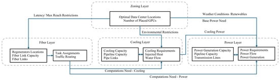
Although each layer has its own objective and constraints, the model is solved as a single integrated optimization model in which decisions propagate across layers through shared decisions. Figure 1 depicts these layers and their interactions. In the proposed framework, the decisions start with the master zoning layer when sitings and GPU assignments are defined after exchanging information with the fiber, cooling, and power layer. Required computations, traffic flow feasibility, latency considerations, cooling demand, water availability, environmental considerations like heat injection limits, and transmission system capacity are critical factors in determining the best siting decisions. Since changes in any of these factors and siting decisions simultaneously affect other variables, they are solved at the same time instead of sequential solving.

Figure 1. Overview of decisions and layer interactions.

In fact, the proposed model considers all interactions between zoning considerations, fiber/optical layer requirements, cooling needs and the water network, and power grid features at the same time. Sequential solving of the model or single-layer optimization without including cross-layer interactions can lead to infeasible or suboptimal siting decisions. For example, considering only zoning requirements can lead to a siting decision with a cheaper and more convenient location, but providing fiber, cooling, and power support for this location might be challenging or impossible.

3.1. Master Zoning Layer

The objective function in the zoning layer minimizes the total fixed cost for placing data centers and variable costs for installing GPU capacities.

$$Z^{Zone}={\displaystyle \sum _{i=1}^I}{F}_i^{DC}{x}_i+{\displaystyle \sum _{i=1}^I}{F}^{GPU}{y}_i$$

(1)

This layer is subject to the following constraints:

$$G^{min}{x}_i\le y_i\le G^{max}xi\forall i$$

(2)

$$x_i\le Z_i\forall i$$

(3)

$$B_1{y}_i\le (B_i^{Ave}-B_0)x_i\forall i$$

(4)

$$N{y}_i-\pi R_i\le N_i^{lim}+M(1-x_i)\forall i$$

(5)

Equation (2) defines limitations for GPU placement for opened data centers. Opening these centers is economically justified by placing limits on the minimum number of installed GPUs. On the other hand, increasing these GPUs from certain limits decreases their efficiency. There are some zoning factors such as local resistance, high levels of humidity and heat level, flood, and other extreme risks that prevents placing data centers in certain nodes of the network (Equation (3)). Depending on the availability of land in some areas, the number of GPUs installed in each location is limited. This limitation is enforced in Equation (4) for the base area of the data center and the area for placing GPUs. Cooling towers produce noise in data centers that can make them annoying for local people. This noise is equivalent to the computation limits of these centers expressed in terms of GPUs installed and the distance between the center and residential areas. Noise impact decreases by increasing the distance from residential areas. Equation (5) ensures that these considerations are included in the model to limit noisy data centers close to residential areas.

3.2. Fiber/Optical Layer

The nest layer is related to fiber infrastructure modeling and its traffic routing. The model for this layer is listed below:

$$Z^{Fiber}={\displaystyle \sum _{i=1}^I}{F}^{Reg}{r}_i+{\displaystyle \sum _{k=1}^K}{F}^{Pen}(1-s_k)+{\displaystyle \sum _{i=1}^I}{\displaystyle \sum _{j=1}^I}{F}^{Fbr}{u}_{ij}^{Fbr}+{\displaystyle \sum _{i=1}^I}{\displaystyle \sum _{j=1}^I}{F}^{Fln}{D}_{ij}{a}_{ij}^{Fbr}+{\displaystyle \sum _{k=1}^K}{\displaystyle \sum _{i=1}^I}{\displaystyle \sum _{j=1}^I}{F}_{ij}^{Rt}{D}_{ij}{f}_{ij}^k$$

(6)

Constraints:

$$c_i^{Com}={\displaystyle \sum _{k=1}^K}{v}_{ik}{C}_k\forall i\in I^{DC}$$

(7)

$$c_i^{Com}\le \beta y_i\forall i\in I^{DC}$$

(8)

$${\displaystyle \sum _{k=1}^K}{f}_{ij}^k\le u_{ij}^{Fbr}\forall i,j$$

(9)

$${\displaystyle \sum _{j=1}^I}{f}_{ji}^k{\displaystyle \sum _{j=1}^I}{f}_{ij}^k=\left\{\begin{array}{cc}-C_k{\gamma }_k{s}_k\hfill & \mathrm{if}i=S\left(k\right),\hfill \\ C_k{\gamma }_k{s}_k\hfill & \mathrm{if}i=T\left(k\right)\in I^{Hb},\hfill \\ v_{ik}{C}_k{\gamma }_k\hfill & \mathrm{if}i\in I^{DC},\hfill \\ 0\hfill & \mathrm{otherwise},\hfill \end{array}\right.\forall i,k$$

(10)

$$z_{ijk}\le f_{ji}^k\le M{z}_{ijk}\forall i,j$$

(11)

$$u_{ij}^{Fbr}\le M(A_{ij}^{Fbr}+a_{ij}^{Fbr})\forall i,j$$

(12)

$${\displaystyle \sum _{i=1}^I}{v}_{ik}=s_k\forall k$$

(13)

$${\displaystyle \frac{{\sum }_{i=1}^I{\sum }_{j=1}^I{f}_{ij}^k\left(\frac{D_{ij}}{\rho }\right)}{C_k}}\le L_k\forall k$$

(14)

$$l_j^k\ge l_i^k+D_{ij}-M(1-z_{ijk})-M{r}_j\forall i,j$$

(15)

$$l_i^k\le R^{Mx}(1-r_i)+\epsilon r_i\forall i,k$$

(16)

The fiber network capacity can increase support data center traffic by adding regenerators to some nodes or increasing fiber line capacity by adding wavelength or upgrading their modulation formats. The costs for these upgrades and routing are reflected in Equation (6). Total computation of each data center node is calculated in Equation (7). Equation (8) ensures that this computation is less than the total computation capacity of each data center defined by its installed GPUs. Equation (9) limits the total traffic passing from each link for all demand-DC pairs to be less than the designed capacity. For every node in the network, flow conservation ensures that incoming traffic is equal to outgoing traffic except for the source and sink node for the traffic (Equation (10)). This equation is designed to reflect any form of routing including demand center to data centers, data centers requesting training services from other data centers, and sending or receiving services from and to hub nodes (IXPs, cloud gateways) by data centers. For source nodes demanding services, the equation injects total traffic generated by residential or industrial areas. For destination nodes such as hubs, the constraint absorbs incoming backbone traffic associated with metro ingress/egress and cloud gateway connectivity. For AI data centers, the equation simultaneously accounts for east–west training flows, multi-site gradient exchange, and proportion of service assigned to the data centers. These assignments are reflected by the variable v in the equation.

Traffic can be routed over many paths and tasks can be split across multiple data centers in this model. Equation (11) is designed to introduce an artificial binary variable that shows if flows exist in certain links or not. Flow capacity is defined only for the existing fiber links shown in the network’s adjacency matrix (Equation (12)). Equation (13) ensures that the computation distributed between multiple data centers is fully assigned and is equal to one. There is also a limit in each service that ensures the average latency is below certain values (Equation (14)). The latency for each fiber line is equivalent to its length and propagation speed in fiber. In long haul optical networks signals, signals must be regenerated after maximum reach. Equations (15) and (16) are designed to guarantee that the total length of links used by commodity k between its source and sink does not exceed some effective reach unless they are reset by regenerators. In this formulation, each service is identified by commodity k where its passed cumulative distance should remain under certain limits. This cumulative distance is reset by placed regenerators given boosted service quality in the nodes with this equipment. This ensures that the total optical distance between consecutive regenerators never exceeds the maximum allowed reach to fully capture the physical behavior of long-haul optical transmission.

3.3. Cooling Layer

The next layer is the water pipeline network that includes the cooling mechanism of the data centers. This layer is modeled using the following equations:

$$Z^{Cool}={\displaystyle \sum _{i=1}^I}{F}^{LC}{u}_i^{LC}+{\displaystyle \sum _{i=1}^I}{F}^{EC}{u}_i^{EC}+{\displaystyle \sum _{i=1}^I}{\displaystyle \sum _{j=1}^I}{F}^{Pipe}{u}_{ij}^{pip}+{\displaystyle \sum _{i=1}^I}{\displaystyle \sum _{j=1}^I}{F}^{Pln}{D}_{ij}{a}_{ij}^{pip}+{\displaystyle \sum _{i=1}^I}{F}^{LO}{c}_i^{LC}+{\displaystyle \sum _{i=1}^I}{F}^{EO}{c}_i^{EC}$$

(17)

Constraints:

$$w_i^{draw}+{\displaystyle \sum _{j=1}^I}{f}_{ji}^{wtr}-{\displaystyle \sum _{j=1}^I}{f}_{ij}^{wtr}=w_i^{Cool}+W_i^{Use}\forall i$$

(18)

$$w_i^{draw}\le W_i^{Ave}\forall i$$

(19)

$$w_i^{Cool}\le W_i^{lim}\forall i$$

(20)

$$f_{ij}^{wtr}\le u_{ij}^{pip}\forall i$$

(21)

$$u_{ij}^{pip}\le M(A_{ij}^{Cool}+a_{ij}^{pip})\forall i,j$$

(22)

$$w_i^{Cool}={\phi }^{LC}{c}_i^{LC}+{\phi }^{EC}{c}_i^{EC}\forall i$$

(23)

$$c_i^{LC}\le u_i^{LC}$$

(24)

$$c_i^{EC}\le u_i^{EC}$$

(25)

$${\delta }^{LC}{c}_i^{LC}+{\delta }^{EC}{c}_i^{EC}\le H_i\forall i$$

(26)

$$u_i^{LC}+u_i^{EC}\le M{x}_i\forall i$$

(27)

$$u_i^{LC}+u_i^{EC}\ge H^{GPU}{y}_i+H^{Base}{x}_i\forall i$$

(28)

$$c_i^{LC}+c_i^{EC}=Q{x}_i+{\alpha }^{Cool}{c}_i^{Com}\forall i$$

(29)

In the above model, water-related variables ($f_{i,j}^{wtr},w_i^{Cool}$) are expressed in volumetric flow units (lit) while other variables such as cooling demand, heat injection, and installed capacity ($c_i^{Cool},h_i,u_i^{wtr}$) are expressed in power units (kW) with conversion factor linking them. The objective function in Equation (17) reflects investments in the installed cooling capacities in nodes and water pipeline capacities. It also includes total cost of providing cooling for the network using both liquid and evaporative technologies. Water flow balance equations considering local water availability and water usage for cooling are reflected in Equation (18). Water draw from local water sources is limited by their availability in each node (Equation (19)). The model includes both evaporative and liquid cooling mechanisims. Evaporative cooling is water-intensive and constrained by node-level water availability, while liquid cooling is a closed loop system with minimal make up water requirements. This dual representation allows the optimization to select feasible cooling strategies under varying hydrological conditions. In each zone, there are certain environmental considerations that limit the water usage for cooling the data centers (Equation (20)). Equation (21) limits the flow in each pipeline by its flow capacity. Pipeline capacities are defined only for existing links shown by the water network’s adjacency matrix (Equation (22)). Equation (23) calculates water used for cooling in both technologies. Total cooling demand of each node should be less than its cooling capacity availability (Equations (24) and (25)). There are limitations on heat injections created using both technologies which are reflected in Equation (26). The cooling capacity is considered only for nodes with data centers (Equation (27)), and it should be more than the required emergency capacity, which is the sum of the fixed and variable heat generation in each center for emergency cases (Equation (28)). Actual cooling is defined in Equation (29) based on the required base cooling and cooling for the received computation.

3.4. Power Layer

The objective function for the power network is listed below:

$$Z^{Power}={\displaystyle \sum _{i=1}^I}{F}^{Gen}{u}_i^{Gen}+{\displaystyle \sum _{i=1}^I}{\displaystyle \sum _{j=1}^I}{F}^{Line}{u}_{ij}^{Flw}+{\displaystyle \sum _{i=1}^I}{\displaystyle \sum _{j=1}^I}{F}^{Trn}{D}_{ij}{a}_{ij}^{Trn}+{\displaystyle \sum _{i=1}^I}{F}^{Gen}{p}_i$$

(30)

Constraints:

$$f_{ij}^p=S_{ij}({\theta }_i-{\theta }_j)\forall i,j$$

(31)

$$p_i\le u_i^{Gen}\forall i$$

(32)

$$-u_{ij}^{Flw}\le f_{ij}\le u_{ij}^{Flw}\forall i,j$$

(33)

$$u_{ij}^{Flw}\le M(A_{ij}^{Flow}+a_{ij}^{Trn})\forall i,j$$

(34)

$${\displaystyle \sum _{j=1}^I}{f}_{ji}-{\displaystyle \sum _{j=1}^I}{f}_{ij}-p_i-P_i+e_i+c_i^{Cur}=0\forall i$$

(35)

$$e_i=E_i^{Base}+e_i^{DC}\forall i$$

(36)

$$e_i^{DC}=D^{Base}{x}_i+{\alpha }^{Power}{c}_i^{Com}+{\pi }^{LC}{c}_i^{LC}+{\pi }^{EC}{c}_i^{EC}\forall i$$

(37)

The objective function in Equation (30) calculates the cost of creating a power generation capacity and the expansion of transmission lines to increase the power flow limit, plus the total cost of power generation. Equation (31) is the DC power flow defined based on the voltage angles connected to the from-bus and the to-bus. Power generation in each bus is limited by its capacity (Equation (32)). Equation (33) ensures that power flow in each transmission line is within the capacity considered for power flow. The capacity is defined only for existing transmission lines shown by the grid network’s adjacency matrix (Equation (34)). Power flow balance between nodes is shown in Equation (35) considering power generation and consumption in each node. The total power in each node includes the residential or industrial base load and the power required for data centers (Equation (36)). Power consumption in data centers is a summation of the base energy and the energy required for computations and the cooling of the data center (Equation (37)).

The proposed multi-layer network is solved by integrating all objective functions subject to all constraints in these layers and setting a minimum number of data centers that we are planning to build.

$$Z=Z^{Zone}+Z^{Fiber}+Z^{Cool}+Z^{Power}$$

(38)

$$\sum _{i\in I}{x}_i\ge 2$$

(39)

The last equation is added to the model to ensure at least two candidates are selected to place the data centers. This setting can be adjusted to reflect a baseline planning of technical requirements for redundancy and operational resilience or strategic goals of the decision makers.

4. Case Study

The efficiency of the proposed model is evaluated in a set of experiments and sensitivity analysis scenarios. These experiments are implemented in a modified 14-Bus IEEE test system with 14 different nodes. Settings for costs and parameters are listed in Table 1 and Table 2. The parameter ranges reported in these tables are collected from industry reports [29,30,31,32,33] and peer-reviewed studies [5,20,34]. In model settings, the electrical parameters follow the standard IEEE Bus transmission settings and the additional settings for cooling, water and fiber layers were extended using physically justified land use and infrastructure logics and simulated scenarios consistent with the under-lying power transmission layer.

Table 1. Cost settings of the model.

Parameter	Setting
Fixed cost of opening DC ($F_i^{DC}$ )	8000–25,000 $k
Cost of placing each GPU ($F^{GPU}$ )	30 $k per GPU
Fixed cost of enabling regeneration	50 $k per site
Cost per fiber capacity (wavelength/Gbps)	5 $k per 100 G
Cost of routing traffic on fiber link ($F^{RT}$)	0.05 $k per Gb/s on km
Cost per kW cooling capacity ($F^{Cool}$ )	1 $k per kW
Cost per unit pipe capacity ($F^{Pipe}$ )	0.05 $k per (lit/h)
Cost of providing cooling ($F_i^C$)	0.5 $k per kW used
Cost per kW generation capacity ($F^{Gen}$)	0.5 $k per kW
Cost per kW transmission upgrade ($F^{Line}$)	0.5 $k per kW
Variable cost of power generation ($F_i^G$)	0.05 $k per kWh
Fixed cost of adding new transmission line	50$ per km
Fixed cost of adding new pipeline	100$ per km
Fixed cost of adding a new fiber line	20$ per km

Table 2. Parameter settings of the model.

Parameter	Setting
Base area per DC	2000 m2
Base DC load	100 kW
Extra area per GPU	1 m2/GPU
Noise per GPU	50 dB/GPU
Noise reduction per km	60 dB/km
Compute capacity per GPU	1 compute units/GPU
Propagation speed in fiber	200 km/ms
Max reach without regeneration	100 km
Fixed cooling requirement	100 kW
Heat per GPU	0.08 kW/GPU
Base heat per DC	100 kW

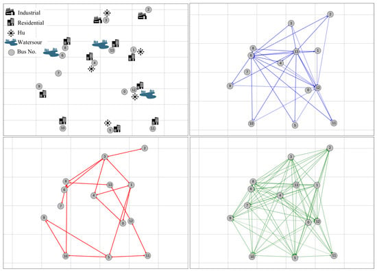
In the case study set up, the parameters are generated based on the 14-Bus IEEE case through a structured role-based mapping of technical features of the case into multi-layer settings for the fiber, zoning, and water network. Technical features of buses such as their load magnitude, generator location, voltage level, and graph features such as node degrees classified them into residential, industrial, power plants, hubs, and DC candidates. Spatial coordinates are generated based on a weighted Kamada–Kawai layout to generate distance-based settings such as fiber reach, pipeline connections, adjacency metrics, and residential proxy. Other than water sources, which are selected randomly from existing buses, other environmental and resource parameters are calculated based on bus types and their categories. The fiber communication layer is constructed using distance-based connectivity rules that reflect the expected deployment density of different node types. Base energy usages are set to normal loads defined in the IEEE cases while renewable availabilities are generated randomly for a limited number of buses in the transmission system suitable for renewable energy injection. Noise limits reflect standard zoning practice with strict thresholds for residential nodes, moderate limits for industrial nodes, and loose thresholds for the remaining places. Heat-injection limits also follow similar zoning limits with industrial nodes tolerating higher thermal loads. Zoning permission restrictions are set only for residentials with 25% chance of getting accepted by people living on that residence. These rules are set to generate parameters consistent with both engineering practice and multi-layer infrastructures in data siting problems. The resultant multi-layer network based on these rules for the 14-bus IEEE case is presented in Figure 2.

Figure 2. IEEE 14 Network; zoning layer (upper left), water layer (upper right), power transmission layer (lower left), and fiber layer (lower right).

The AI data centers in this research will support the county with 4 different classes of services (Figure 2). Class A inferences services are dedicated to traffic from demand centers to data centers that residential/industrial areas send their AI queries such as search, user prompts, chatbots, factory analytics, and automations to the available data centers. This class is latency-sensitive and light in bandwidth. Class B of the traffic is known as east–west traffic between AI data centers for model training, gradient synchronization, check points, replications, and distributed computation. This class is bandwidth-intensive, has a long duration, and is latency-tolerant. Class C of the traffic is between hubs and data centers and includes hubs/IXPs/cloud gateways used for the county’s incoming or outgoing traffic and connecting the county to national and global networks. The reverse traffic from data centers to some edge/storage/regional small-scale data centers is a small proportion of traffic labeled as Class D and mostly is used for caching, backup, replication, and low-latency inference offload. Each service is instantiated by sampling its class type, selecting an origin node from the corresponding node category, and assigning its destination dynamically through the optimization model based on the optimal data-center selection. For the first three classes of traffic, the origin nodes are selected randomly while the destinations are determined in the model based on the optimal service assignments between data centers. A certain portion of requests per node is modeled to reflect similar county-level AI services in a representative peak hour with traffic simulated based on the ratios and distributions listed in Table 3. The computation requirement is simulated using lognormal distributions to reflect realistic network demand consistent with empirical observations in fiber networks [35]. Latency and other service parameters are simulated using uniform distributions to ensure existing variabilities in traffic without adding unnecessary complexities to the model.

Table 3. Traffic variations and settings.

Traffic Class	Service Ratio	Compute Requirement (${\mathit{C}}_{\mathit{k}}$)	Traffic per Compute (${\mathit{\gamma }}_{\mathit{k}}$)	Latency Tolerance (${\mathit{L}}_{\mathit{k}}$)
A	60%	Residentials: Lognormal (50, 0.5)	Uniform (0.1, 1)	10 ms
		Industrial: Lognormal (200, 0.6)
B	25%	Lognormal (1000, 0.8)	Uniform (100, 300)	50 ms
C	10%	Lognormal (500, 0.7)	Uniform (10, 50)	20 ms
D	5%	Lognormal (1000, 0.7)	Uniform (1, 20)	30 ms

The model is run on a desktop equipped with an Apple M4 Pro14 Core CPU, 20 core GPU, and 24 GB RAM with macOS 26.6.2. The model is coded in Python 3.10 and is solved using IBM CPLEX 22.1 solver. The computation time, optimality gap and model size are reported in Table 4. The result for the default case study is presented in Table 5.

Table 4. Computation details of the model for default case.

Computation Time (s)	Optimality Gap	Total Constraints	Binary Variables	Total Variables
0.9375	0	68,027	21,410	46,028

Table 5. Results for default case study.

Total Cost ($k)	Siting Nodes	Total GPU Installed	Service Rate	Water Usage (lb)	Fiber Operations Costs ($k)	Power Operations Costs ($k)
4,262,076	0 and 7	8428	80%	8628	10,135	569

These results showed that adding two fiber links to the network helps the system to achieve better results while other water and power networks stay unchanged. This is mainly because cooling systems mostly rely on local capacities rather than global connections with the rest of the network. Based on the results, the links connecting data centers to demand centers forced them to increase their capacities, and these capacity investments are mostly in links connected to the power generation nodes of the power network.

5. Results

To analyze the effects of various settings on siting decisions, a complete set of experiments is designed and run to record the behavior of the model in different scenarios.

5.1. Noise Effects

One of the influencing factors in data center siting decisions is the effect of noise on close-by residential areas. These limits are usually set locally through municipal noise ordinances, zoning setbacks, and permit-specific conditions. This is especially important for AI data centers as their cooling and backup systems run 24/7, disturbing nearby residential areas. To check the effects of such settings on total costs, we set different levels of noise limits as shown in the table. To capture noise effects, we set up residential and industrial noise limits of 40 and 70 accordingly and 5000 for the rest of the nodes. The results for these experiments are listed in Table 6:

Table 6. Results for changing noise restriction levels.

Noise Setting	Total Cost	Selected Nodes	GPUs
20X Increase	$6,366,143	0, 7	4003
10X Increase	$8,979,862	0, 7	2005
5X Increase	$10,903,705	0, 7	1005
Default	$13,146,991	0, 7	200
20% Decrease	Infeasible	-	-

The results suggest that reducing noise restrictions decreases the related costs of data center siting decisions, but these changes do not change the node selections of the data centers. This is mainly because only certain nodes are at an adequate distance from residential and industrial areas and these changes can only affect GPU installation decisions of the system.

5.2. Latency Effects

Service latency is unavoidable due to traffic flow in fiber networks. Latency requirements for various levels are tested to see if they have a significant influence on infrastructure and operation costs of the system. The latency considerations in this model focus on propagation delay, which is the influencing factor in wide-area fiber networks and their placement decisions. Other types of latencies such as processing, transmission, queueing, and switching delays are not included in the model. This is mainly because these delays are not significant and they are independent of the geographical layout of the network. To analyze the effects of propagation delays, the threshold level is changed for all four different service types at the same level, and the model is solved with and without possibility of placing regenerators. Table 7 summarizes the results for these experiments where default settings are slightly modified to capture latency effects.

Table 7. Cost results for changing latency restrictions with and without placing regenerators.

	Without Regenerators			With Regenerators
Latency Setting	Total Cost	Routing Cost	New Links	Total Cost	Routing Cost	New Links
50% Increase	$63,384,486	$5,051,862	11	$63,257,970	$4,952,806	10
20% Increase	$57,725,157	$4,205,688	9	$57,609,937	$4,197,293	8
Default	$56,480,330	$3,564,142	7	$56,367,595	$3,557,028	6
20% Decrease	$53,763,627	$3,368,114	5	$53,656,314	$3,361,391	3
50% Decrease	$48,968,447	$3,166,027	2	$48,008,281	$3,159,708	0

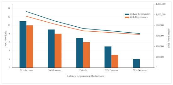
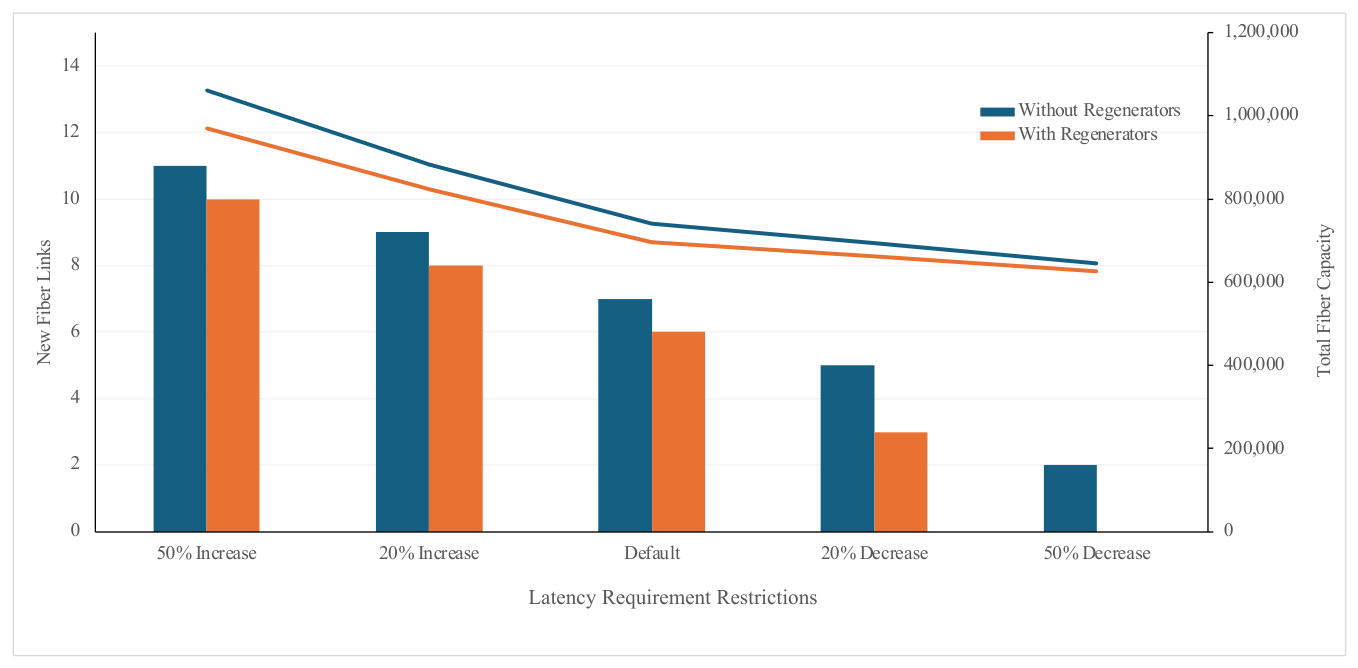
In each experiment, all latency limits are changed for all four different service types at the same level, and the model is solved to record the results of new settings with and without placing regenerators. The capacity changes for the fiber links are shown in Figure 3:

Figure 3. Topology and capacity change for different levels of latency restrictions.

Results show that latency requirements reshape fiber network topology more than changing GPU installations in data centers. Regenerators are like local enablers that remove increasing routing costs and force shorter links to be placed to preserve the latency requirements of the supported services.

5.3. Natural Effects

The effect of nature on data centers is another important factor that can influence data center siting strategies. Abundant water availability determines if a center can support the cooling of the center without stressing local rivers or aquifers. Similarly heat level can also limit heat injection and increase cooling costs of the data centers. In cooler climates with stable freshwater supplies, data centers can operate more efficiently.

Data centers can be supported by renewable energies and the potential of using such low-cost resources can affect the siting decisions of these centers. Utilizing green energy can also influence community resistance by reducing the negative environmental effects of these centers. These effects are checked in the three following scenarios:

• Water scarcity: decreasing water availability in all sites to half of the current setting.
• Heat restriction: reducing heat injection level by 50% due to high temperatures in candidate sites.
• Renewables restriction: Reducing renewable energy availability by 50% due to weather changes.

The results for these scenarios are summarized in Table 8.

Table 8. Results for simulating nature effects.

Scenario	Total GPU	Total Cost	Total Cooling Cap	Total Generation Cap
Default	300	$56,367,595	216	88,500
Water Scarcity	6200	$60,877,002	320	90,100
Heat Restriction	5500	$62,185,200	420	96,830
Renewables Restriction	5840	$58,993,202	228	95,458

In these nature-effect-related scenarios, the network responded by reshaping the network structure and changing computation placements. Water scarcity pushes data centers toward nodes close to water resources and requires increased cooling capacities in these centers. Similarly pipelines and routings are adjusted to meet the required cooling capacity. This scenario increases the total cost by 8%. Heat restriction is another disrupting factor that forces data centers to spread their cooling resources thinner. As a result, transmission and power generation upgrades are needed to support such cooling systems. Weather changes and restrictions in the availability of renewables forces data centers to be at sites close to power generation nodes and increase their power generation. All nature-related factors trigger network-level adaptations and increases in total infrastructure and operation costs of the system.

5.4. Effects of Traffic Splitting

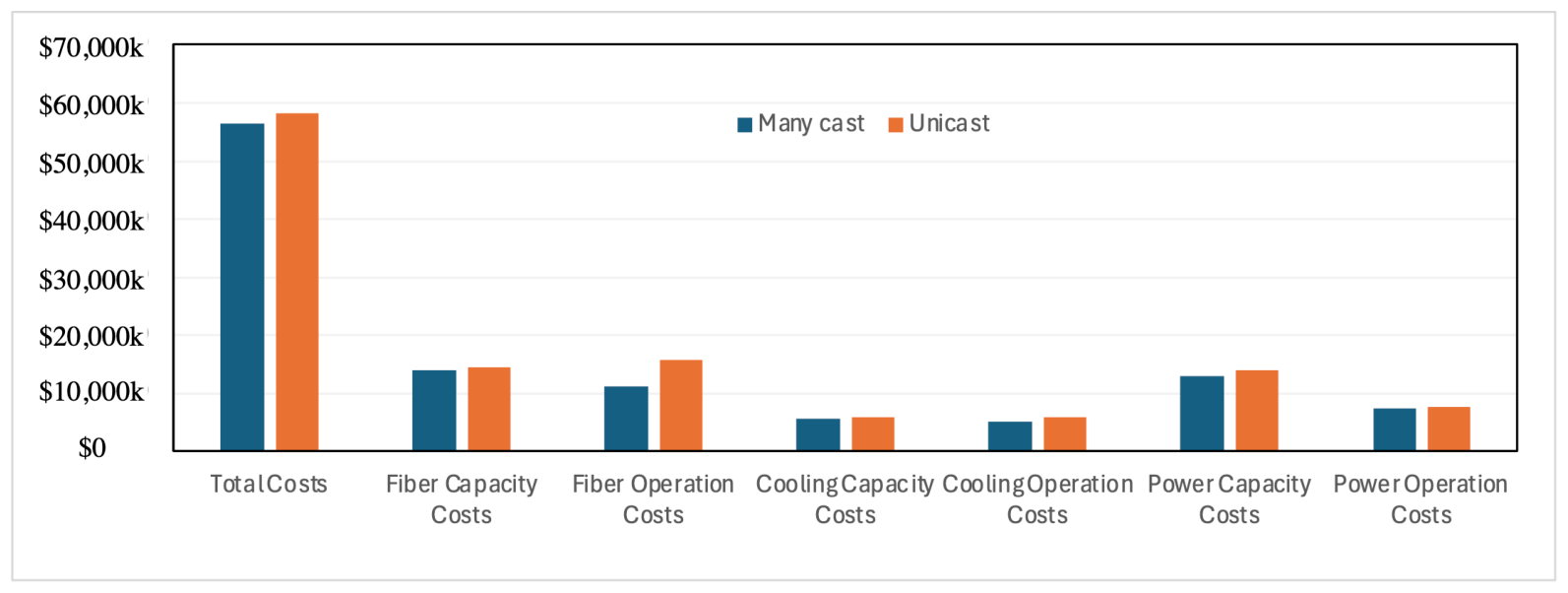
We also tested unicast versus many-cast scenarios in the proposed model by restricting traffic routing and splitting in the network. In the unicast scenario, traffic for different services cannot be split between multiple data centers. This condition is set by adding the following constraints:

$${\displaystyle \sum _{j=1}^I}{z}_{i,j,k}=1\forall i,k$$

(40)

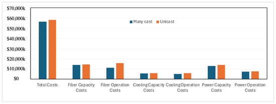
Different costs for both scenarios are reflected in Figure 4:

Figure 4. Results for comparing many-cast versus unicast traffic routing.

As the results show restricting optical network flow to unicast slightly increases the cost of placing power generation in more dense nodes and increases optical network routing costs due to less parallel, cheaper routes.

5.5. Uncertainty Effects

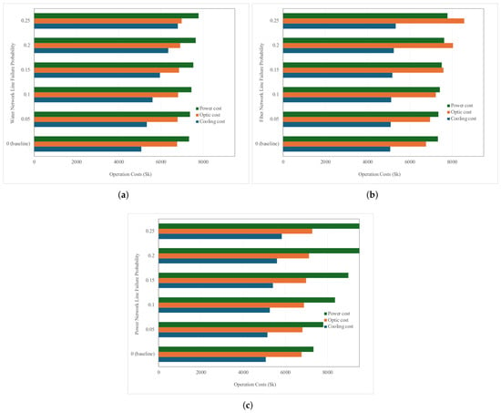
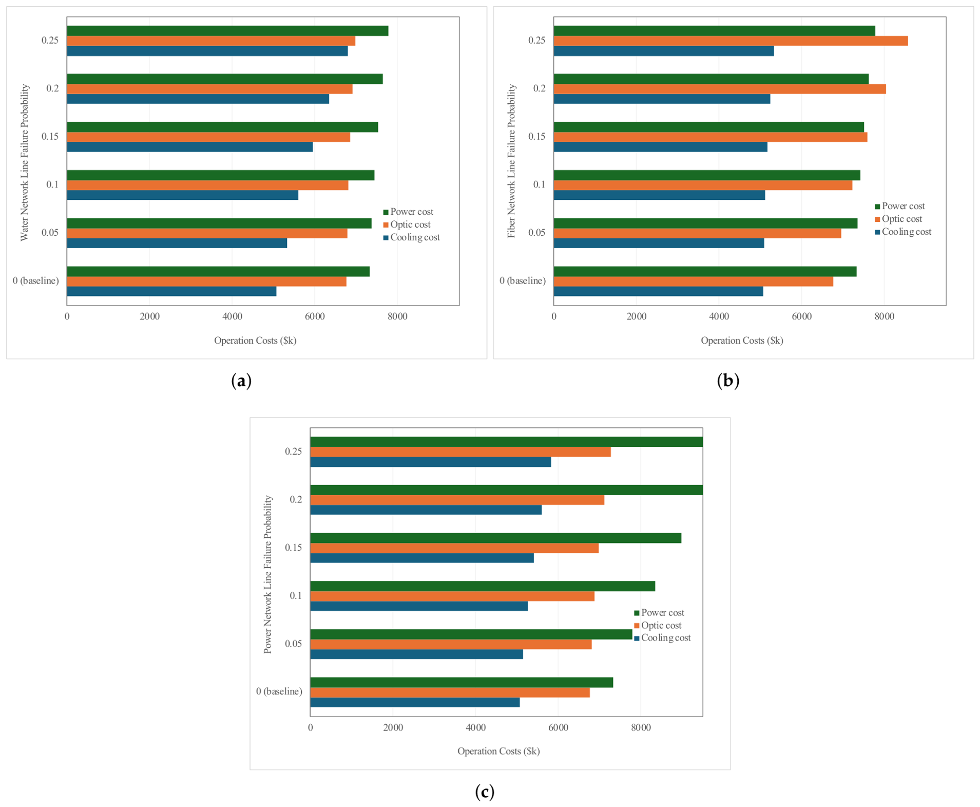
One of the most influential factors is the effect of the uncertainty of the successful operation of data centers. To investigate uncertainty effects such as failures, a set of experiments is implemented by removing random links of the networks from each layer and recording how operation costs are affected when the data center system and its related element are set based on the optimized variables. It is assumed that these failures happen with equal probability for all links. Figure 5 presents the results.

Figure 5. Operation costs changes in different failure scenarios: (a) Water pipeline failure scenarios. (b) Fiber link failure scenarios. (c) Transmission line failure scenarios.

The results show that any failure in the water network forces the rerouting of water and the activation of expensive cooling options and in some cases loosening cheap computation capacities. These changes are small, because water networks are mostly local variables and are mostly affected by local factors. These changes are more visible in optical network failures, because any failure in the optical network changes the computation hosts and forces longer paths, and, as a result, increases routing costs. These changes may require placing more expensive regenerators to ensure the feasibility of services with the required latency limits. Changing computation hosts also increases power generation costs in expensive options. The fiber network is a workload distribution backbone and any failure in this layer significantly increases the operation costs of the system. Similarly, failures in transmission lines increase power operation costs sharply by using more expensive power plants and expensive computation hosts.

5.6. Scalability Test

To ensure that the proposed framework is also applicable for larger networks, it was run on larger IEEE cases in the existing library. The results for computation times and other technical considerations are reported in Table 9 and are compared with the default case with 14-bus setting. As the results show, increasing network size considerably increases the computation time of the system and we may need to use meta-heuristics to find suboptimal solutions.

Table 9. Computation details of the model for default case.

Case	Computation Time (s)	Optimality Gap	Total Constraints	Binary Variables	Total Variables	Total Cost
IEEE 14-Bus	0.9375	0	68,027	21,410	46,028	4,262,076
IEEE 39-Bus	779	1.523 × 10−5	1,575,264	515,400	1,061,713	25,778,670
IEEE 57-Bus	1869.95	0.000209	5,239,690	1,726,044	3,518,179	27,466,564

6. Conclusions and Future Work

This research proposes an integrated decision-making framework for placing county-level AI data centers considering various cooling, zoning, fiber, and power grid network factors. The proposed multi-layer network optimization framework jointly models zoning considerations for noise and local restrictions, fiber routing, water cooling feasibility, and power grid capacities to find the best locations for data centers while minimizing current investment and future operation costs of the system. Various experiments were implemented to determine effects of nature, costs, settings, and uncertainties on network capacity and topology decisions. The findings highlighted the importance of coordinating various decisions for utilities, fiber operators, and cloud providers who face shared constraints such as grid congestion, water stress, land scarcity, and latency requirements. This framework provides several practical implications for stakeholders involved in regional AI infrastructure planning. For utility operators, the model highlights how GPU-driven load growth, cooling water demand, and noise constraints influence substation upgrades and feeder reinforcement. Network providers can use the fiber routing and latency outputs to identify where east–west AI traffic will concentrate and where additional backbone capacity or diverse paths are needed. Municipalities benefit from the siting recommendations that balance industrial zoning, residential noise tolerance, and water availability, helping them evaluate land use compatibility and permitting considerations. For data center planners, the integrated power-fiber-water optimization offers guidance on selecting sites that minimize operational constraints while ensuring scalable connectivity and sustainable resource usage. Together, these insights translate the optimization results into actionable planning signals for real deployments.

The current research can be extended by incorporating future uncertainties during initial investment decisions using techniques such as two-stage stochastic programming to capture effects of factors such as link and node failures in networks, traffic and load fluctuations, and extreme weather events that can significantly affect the cooling and power generation decisions of the network. Considering path redundancies in routing decisions of the optical network can be also added to the model to increase the reliability of the proposed data center siting decisions. The proposed method was used as a basis for real-time planning of data center networks for traffic routing, power generation and cooling decisions and when the system faces frequent fluctuations in different layers and has to respond quickly while considering its effects on other related decisions and outcomes. One of the limitations of this research is that it considers independent link failures for robustness analysis which only reflect a simplified version of real-world outages. Future work can extend this idea by including more correlated failures to show regional natural disasters and analyze the effects of these events on data center siting decisions and network infrastructure adjustments.

References

- Chen, D.; Zhou, Z.; Cai, Y.; Qin, J.; Katchova, A.; Chen, L. Concentrated siting of AI data centers drives regional power-system stress under rising global compute demand. arXiv 2026, arXiv:2604.06198. [Google Scholar]
- Ran, Y.; Zhou, X.; Hu, H.; Wen, Y. Optimizing data center energy efficiency via event-driven deep reinforcement learning. IEEE Trans. Serv. Comput. 2022, 16, 1296–1309. [Google Scholar] [CrossRef] [Scilit]
- Davenport, C.; Singer, B.; Mehta, N.; Lee, B.; Mackay, J.; Modak, A.; Corbett, B.; Miller, J.; Hari, T.; Ritchie, J.; et al. AI, data centers and the coming US power demand surge. Goldman Sachs 2024, 26, 10–20. [Google Scholar]
- Xiao, X.; Jiang, S.; Zheng, Z.; Zhang, M.; Chen, Y.; Chen, X. Integrated decision-making methodology for low-carbon data center siting, dispatch, and transmission based on wind-solar-hydro-computing synergy. IEEE Trans. Ind. Appl. 2026. [Google Scholar] [CrossRef] [Scilit]
- Vabson, M.; Zater, M.E.; Sajadi, A.; Baker, K.; Hodge, B.-M. Optimal County-Level Siting of Data Centers in the United States. arXiv 2026, arXiv:2601.16315. [Google Scholar]
- Kseibati, R. Cooling Innovation and Circularity: Addressing Water Stress in the Age of AI-Driven Data Centers. Ph.D. Thesis, Massachusetts Institute of Technology, Cambridge, MA, USA, 2025. [Google Scholar]
- Wu, Y.; Li, Z.; Wang, Y.; Feng, Q.; Zhao, J.; Liu, S. Optimizing Data Center Locations: A Bi-level Approach. In Proceedings of EIECS 2025; IEEE: New York, NY, USA, 2025; pp. 1318–1321. [Google Scholar]
- U.S. Department of Energy. Grid Modernization Initiative; U.S. Department of Energy: Washington, DC, USA, 2023. Available online: https://www.energy.gov/gmi (accessed on 25 June 2026).
- Sticca, G.S.; Ibrahimi, M.; Musumeci, F.; Di Cicco, N.; Tornatore, M. Hollow-core fibers for latency-constrained and low-cost edge data center networks. IEEE Trans. Netw. Serv. Manag. 2025, 23, 443–455. [Google Scholar] [CrossRef] [Scilit]
- Agarwal, A.K.; Kaur, H.; Rakesh, N.; Krishna, K.R.; Dewangan, B.K.; Sahana, S. Energy-efficient optical network design for next-generation data centers. In Proceedings of OPTIMA 2025; IEEE: New York, NY, USA, 2025; pp. 195–201. [Google Scholar]
- Zhu, C.; Yang, S.; Chen, H.; Shao, W.; Wang, X.; Ju, W.; Chen, B. Resource-Level Task Offloading with Adaptive Modulation. In Proceedings of PGC 2025; IEEE: New York, NY, USA, 2025; pp. 1–3. [Google Scholar]
- Baziana, P.A. Optical data center networking: A comprehensive review on traffic, switching, bandwidth allocation, and challenges. IEEE Access 2024, 12, 186413–186444. [Google Scholar] [CrossRef] [Scilit]
- Srikandabala, K.; Prabagar, K.; Jayatilleke, S.; Zhang, P.; Ellerbrock, R.; Rinas, S.; De Silva, D.; Alahakoon, D. Optimization and management of data center networks: A scoping review. IEEE Access 2025, 13, 134699–134720. [Google Scholar] [CrossRef] [Scilit]
- Singh, K.D. Role of optical network in cloud/fog computing. In Telecommunication Systems—Principles and Applications of Wireless–Optical Technologies; IntechOpen: London, UK, 2019. [Google Scholar]
- Marmat, A.; Thankachan, D. Design of an integrated unified intelligence-driven method for low-latency, energy-efficient, and secure cloud-integrated optical broadband access networks. Int. J. Inf. Technol. 2025. [Google Scholar] [CrossRef] [Scilit]
- Chen, L.; Wemhoff, A.P. Characterizing data center cooling system water stress in the United States. In Proceedings of the ASHRAE Annual Conference Papers, Toronto, ON, Canada, 25–29 June 2022. [Google Scholar]
- Mytton, D. Data centre water consumption. npj Clean Water 2021, 4, 11. [Google Scholar] [CrossRef] [Scilit]
- Lazic, N.; Boutilier, C.; Lu, T.; Wong, E.; Roy, B.; Ryu, M.K.; Imwalle, G. Data center cooling using model-predictive control. NeurIPS 2018, 31, 3814–3823. [Google Scholar]
- Li, Y.; Wen, Y.; Tao, D.; Guan, K. Transforming cooling optimization for green data center via deep reinforcement learning. IEEE Trans. Cybern. 2019, 50, 2002–2013. [Google Scholar] [CrossRef] [Scilit] [PubMed]
- Rostami, S.; Down, D.G.; Karakostas, G. Linearized data center workload and cooling management. IEEE Trans. Autom. Sci. Eng. 2024, 22, 3502–3514. [Google Scholar] [CrossRef] [Scilit]
- Siegle, A. The Data Center as a Power Plant. SSRN 2025. [Google Scholar] [CrossRef] [Scilit]
- Haddad, M.; Nicod, J.-M.; Péra, M.-C.; Varnier, C. Stand-alone renewable power system scheduling for a green data center. J. Sched. 2021, 24, 523–541. [Google Scholar] [CrossRef] [Scilit]
- Gao, J.; Wang, H.; Shen, H. Smartly handling renewable energy instability in cloud datacenters. In Proceedings of IPDPS 2020; IEEE: New York, NY, USA, 2020; pp. 769–778. [Google Scholar]
- Ran, Y.; Hu, H.; Wen, Y.; Zhou, X. Optimizing energy efficiency for data center via parameterized deep reinforcement learning. IEEE Trans. Serv. Comput. 2022, 16, 1310–1323. [Google Scholar] [CrossRef] [Scilit]
- Yi, D.; Zhou, X.; Wen, Y.; Tan, R. Toward efficient compute-intensive job allocation for green data centers. In Proceedings of ICDCS 2019; IEEE: New York, NY, USA, 2019; pp. 634–644. [Google Scholar]
- Liang, J.; Chen, D.; Xu, S. Energy-Constrained optimization of data center layouts. Energies 2025, 18, 5040. [Google Scholar] [CrossRef] [Scilit]
- Aziz, A.S.; Emad, M.; Ismail, M.; Rashad, H.; Ali, A.M.; Abdelhafeez, A.; Mohamed, S.S. An Intelligent Multi-Criteria Decision-Making Model for selecting an optimal location for a data center. J. Intell. Syst. IoT 2023, 9, 23–35. [Google Scholar] [CrossRef] [Scilit]
- Li, C.; Yu, X.; Zhao, W.-X. An integrated approach to site selection for a big data center using PROMETHEE–MCGP methodology. J. Intell. Fuzzy Syst. 2021, 41, 6495–6515. [Google Scholar] [CrossRef] [Scilit]
- Cushman & Wakefield. Data Center Development Cost Guide; Cushman & Wakefield: Hong Kong, China, 2026; Available online: https://www.cushmanwakefield.com (accessed on 18 July 2026).
- EIA. Annual Electric Generator Report; EIA: Washington, DC, USA, 2024. Available online: https://www.eia.gov/electricity/generatorcosts/ (accessed on 15 August 2026).
- NVIDIA. NVIDIA H100 Tensor Core GPU Product Specifications and Pricing; NVIDIA: Santa Clara, CA, USA, 2026; Available online: https://www.nvidia.com (accessed on 18 June 2026).
- Zable Cable. Fiber Optical Cable Cost Guide; Zable Cable: Shanghai, China, 2025; Available online: https://zablecable.com (accessed on 21 August 2026).
- Federal Communications Commission. Fiber Infrastructure Cost Benchmarks; Federal Communications Commission: Washington, DC, USA, 2025. Available online: https://broadbandmap.fcc.gov (accessed on 20 August 2026).
- Chen, T.; Wang, X.; Giannakis, G.B. Cooling-aware energy and workload management in data centers via stochastic optimization. IEEE J. Sel. Top. Signal Process. 2015, 10, 402–415. [Google Scholar] [CrossRef] [Scilit]
- Alasmar, M.; Clegg, R.; Zakhleniuk, N.; Parisis, G. Internet traffic volumes are not Gaussian—They are log-normal. IEEE/ACM Trans. Netw. 2021, 29, 1266–1279. [Google Scholar] [CrossRef] [Scilit]
Disclaimer/Publisher’s Note: The statements, opinions and data contained in all publications are solely those of the individual author(s) and contributor(s) and not of MDPI and/or the editor(s). MDPI and/or the editor(s) disclaim responsibility for any injury to people or property resulting from any ideas, methods, instructions or products referred to in the content. |
© 2026 by the authors. Licensee MDPI, Basel, Switzerland. This article is an open access article distributed under the terms and conditions of the Creative Commons Attribution (CC BY) license.