


Abstract
This paper presents a measurement-driven study of end-to-end latency in an indoor private standalone 5G network deployed at TU Wien IFT TEC-Lab. The testbed combines pico radio units, edge computing resources, and a local 5G core to form a campus-scale private network architecture designed for low-latency communication. To characterize network performance, TCP throughput and UDP one-way latency measurements were collected in a single-user, constant-bit-rate downlink setting at seven predefined indoor locations using iPerf-based tests at six traffic levels (1–500 Mbps), with five repetitions per condition. Based on these measurements, a compact parametric model was calibrated for this deployment to describe latency as a function of achieved bandwidth and location-dependent effects. The results show that latency remained low and relatively stable at low and medium traffic levels, generally staying below 20 ms between 1 and 200 Mbps, but increased more strongly as the operating point approached the practical throughput limit of the setup. The fitted model captured the overall latency trend with an in-sample MAE of 2.52 ms, an RMSE of 3.13 ms, and an of 0.842, while retaining comparable predictive performance under a trial-based test split () and leave-one-location-out validation (). The compact model also achieved lower out-of-sample errors than the minimal M/M/1-type and polynomial-regression baselines under both validation schemes. Overall, the findings indicate that traffic load was the main driver of latency growth in the studied environment, while spatial effects remained measurable but secondary. The resulting formulation should be understood as an interpretable empirical model of end-to-end latency for one indoor private standalone 5G deployment under single-user, constant-bit-rate downlink conditions, rather than as a general latency model for private 5G networks. Within that scope, the model provides an interpretable description of the measured latency behavior and a basis for preliminary capacity assessment in this deployment. Its applicability to another private 5G network has not been established and would require a new measurement campaign, complete parameter re-estimation, and independent validation.
1. Introduction
The advent of fifth-generation (5G) wireless networks marks a transformative era in mobile communications, characterized by unprecedented data rates, ultra-low latency, and massive device connectivity. These capabilities are pivotal for supporting a diverse range of applications, including enhanced mobile broadband (eMBB), ultra-reliable low-latency communications (URLLC), and massive machine-type communications (mMTC) [1,2]. In particular, private standalone 5G networks deployed in indoor environments, such as factories, campuses, and hospitals, offer high degrees of control, data privacy, and tailored configuration suited to specific operational requirements [3,4]. These networks are particularly suited for latency-sensitive applications such as augmented reality (AR), virtual reality (VR), industrial automation, and real-time control systems, where stringent quality of service (QoS) requirements must be met [5].
End-to-end latency, defined as the time taken for a data packet to travel from source to destination, is a critical performance metric in 5G networks. It directly influences user experience and the feasibility of applications requiring near-instantaneous response times [5]. For instance, variations in signal strength due to walls or other obstacles, as well as differing bandwidth demands from applications such as video streaming versus IoT sensor data, can significantly impact latency. Accurately predicting latency based on these factors is essential for optimizing network performance, ensuring efficient resource allocation, and meeting the QoS demands of diverse applications.
Despite the importance of latency prediction, the existing literature reveals a significant research gap. While numerous studies have explored latency management and monitoring in 5G networks [5,6,7,8], few have focused on predicting end-to-end latency in indoor private 5G networks using mathematical modeling techniques and machine learning that incorporate user location and application-specific bandwidth requirements [3,4,8]. Existing models often address broader 5G scenarios, such as vehicular communications or public networks, and may not adequately account for the unique challenges of indoor environments, including multi-path fading and signal attenuation due to physical obstructions [8]. This paper addresses this gap using measurements collected at seven distinct locations within the studied private 5G campus deployment to calibrate and validate an empirical latency model for the evaluated operating conditions.
Beyond this application-domain context, the deployment-calibrated model is positioned relative to two research strands identified in the recent literature on 5G latency modeling. As comprehensively surveyed by Mostafavi [8], work on latency prediction and characterization in communication networks broadly divides into abstract queueing-theoretic approaches and data-driven approaches, with recent efforts increasingly bridging the two. Representative examples of the first strand include Coll-Perales et al. [7], who derive a closed-form end-to-end latency model for 5G V2X communications grounded in classical queueing theory, and Abdullah et al. [9], who develop a discrete-time queueing model to compute outage probability for URLLC traffic under heterogeneous radio conditions. Representative examples of the second strand, and of the emerging hybrid direction, include Skocaj et al. [6], who derive the 5G user-plane latency as a Hypoexponential distribution from an M/M/1 queueing formulation and subsequently calibrate it against real network KPIs using machine learning. These studies are methodologically related to the present work but address different application domains, deployment contexts, or modeling objectives. The contribution of the present study does not arise from introducing a new queueing or regression component in isolation. Rather, it lies in integrating a linear traffic term, a physically motivated capacity-saturation term, and a limited additive location adjustment within an interpretable, measurement-driven model for an indoor private standalone 5G deployment. The model is calibrated using end-to-end latency measurements collected at seven indoor locations and is evaluated using both a trial-based train/test split and leave-one-location-out (LOLO) cross-validation. The relative contribution of its components and the trade-off among predictive accuracy, model complexity, and interpretability are examined through the ablation and baseline comparisons presented in Section 5.4. The scope of the resulting model is deliberately narrow. It is an empirical description of end-to-end latency for one indoor private standalone 5G deployment, calibrated under single-user, constant-bit-rate downlink traffic, and it is not proposed as a general latency model for private 5G networks. The fitted parameter values are specific to this deployment and to the measured operating range. The measurement and validation procedure can be repeated in another deployment, but neither the present parameter estimates nor the transferability of the functional form is claimed.
The objectives of this research are threefold:
- 1.
- To document the physical and logical architecture of a private indoor 5G network, including hardware specifications and topological layout.
- 2.
- To collect and analyze UDP one-way latency and TCP throughput data from seven predefined indoor measurement points.
- 3.
- To develop and validate an interpretable empirical latency model for this deployment, using achieved throughput and measurement location as predictors, under single-user, constant-bit-rate downlink conditions.
This paper makes the following contributions:
- It provides a comprehensive overview of the hardware and network layout of TU Wien IFT TEC-Lab private 5G campus deployment, serving as a testbed for latency analysis.
- It introduces a measurement-based methodology that leverages latency and bandwidth data collected via iPerf from seven indoor locations, offering measurement-based insights.
- It proposes and evaluates an interpretable empirical latency model for the studied deployment, using achieved throughput and measurement location as predictors under single-user, constant-bit-rate downlink conditions.
The remainder of this paper is structured as follows: Section 2 details the methodology, providing an overview of the physical and logical architecture of the private 5G campus network used in this study, including a topological map, alongside the experimental setup and measurement configurations. Section 3 presents a statistical analysis of the collected latency and bandwidth data, exploring spatial and application-level variations. Section 4 introduces the mathematical models developed for latency estimation, outlining their theoretical basis, modeling assumptions, and integration of achieved throughput and measurement-location effects. Section 5 discusses the results, comparing estimated latency values with empirical measurements and evaluating model accuracy. Section 6 offers a broader interpretation of the findings, highlights practical implications for the 5G network optimization, and identifies limitations and future research directions. Finally, Section 7 concludes the paper by summarizing the main contributions and outcomes.
2. Methodology
2.1. Network Setup
The private standalone 5G network deployed at the TU Wien IFT TEC-Lab in Vienna, Austria, has a layered architecture comprising radio access, edge computing, core network, transport, and security layers. It integrates commercial-grade ZTE hardware and network-management solutions to support low-latency, high-throughput, and mission-critical communication. The reported configuration values were obtained through the ZTE UME R80 network-management platform and from the technical specifications of the deployed equipment. The exact installed software-release number and procurement location of the equipment were not recorded in the measurement documentation. The entire system operates independently from public mobile networks, offering complete control over configuration, quality of service (QoS), and data privacy.
2.1.1. Radio Access Network Layer (RAN)
The Radio Access Network (RAN) is the primary interface between user equipment (UE) and the 5G network. It manages wireless signal transmission and reception, radio resource scheduling, radio link adaptation, handovers, and baseband processing functions such as modulation and demodulation [10,11,12,13]. The RAN comprises base stations (gNodeBs) that process radio-interface traffic before forwarding it to the core network.
In a typical standalone 5G deployment, the RAN operates on New Radio (NR) frequency bands, such as 3.5 GHz (n78), using advanced antenna technologies like massive MIMO and beamforming to provide high throughput and low-latency connectivity. In contrast, the indoor deployment in this study utilizes ceiling or wall-mounted pico cells to deliver targeted, short-range coverage suitable for dense indoor environments [14].
Figure 1 (Section 2.1.6) illustrates the physical configuration of the indoor RAN, including the interconnection between pRRUs, the P-Bridge, and the baseband unit (BBU) via fiber and hybrid cables, within the overall system architecture. To facilitate reproducibility, Table 1 summarizes the available RAN configuration parameters used during the measurement campaign. The reported values were obtained from the ZTE UME R80 management interface and the technical specifications of the deployed equipment.
Figure 1.
Schematic topology of the TU Wien IFT TEC-Lab private standalone 5G network; three of the seven deployed pRRUs are shown for clarity.
Table 1.
Radio access network configuration used during the measurement campaign.
The parameters reported in Table 1 affect the latency characteristics of the deployment in several ways. First, the configured numerology determines the temporal granularity of radio transmission. For a 100 MHz NR channel with a subcarrier spacing of 30 kHz, the maximum transmission bandwidth configuration comprises 273 PRBs [15]. With this subcarrier spacing (), one NR slot lasts 0.5 ms and one OFDM symbol lasts approximately 35.7 s. Therefore, the physical transmission time of a single datagram represents only a small fraction of the millisecond-scale end-to-end delays observed in the measurements.
Second, the TDD frame structure determines when downlink and uplink transmission opportunities occur. The configured DDDDDDDSUU pattern repeats every 5 ms and contains seven downlink slots, one special slot, and two uplink slots. With six downlink, four guard, and four uplink symbols in the special slot, downlink symbols occupy 104 of the 140 symbols in each 5 ms period, corresponding to a downlink symbol share of approximately 74.3%. The longest interval without a downlink transmission opportunity is 36 symbols, or approximately 1.29 ms. The frame structure can therefore introduce a scheduling component with gaps of up to approximately 1.3 ms to downlink latency, depending on the arrival time of a packet within the TDD cycle. Uplink opportunities are more limited and concentrated toward the end of the frame period; this asymmetry can also influence control signaling and retransmission timing even though the application traffic evaluated in this study was downlink.
Third, the configured bandwidth, PRB allocation, modulation, and MIMO capabilities show that the latency increase observed at the highest traffic level should not be interpreted as direct evidence that the theoretical air-interface capacity was reached. Using the peak-data-rate formulation specified in 3GPP TS 38.306 [16], with 273 PRBs, 256QAM, four spatial layers, and the applicable overhead factor, the configuration yields a theoretical downlink rate of approximately 2.34 Gbps before applying the configured TDD downlink duty cycle. Applying the configured 74.3% downlink symbol share gives an approximate upper bound of 1.74 Gbps with four layers, or approximately 0.87 Gbps with two layers. These values are configuration-dependent theoretical bounds rather than measured data rates because the number of active layers and the instantaneous MCS were not recorded during the campaign.
Q7 achieved the highest location-level mean TCP throughput, at approximately 659 Mbps, while the effective-capacity parameter estimated from the UDP latency measurements was approximately Mbps. Both values are below the theoretical air-interface bounds. Moreover, the measured end-to-end path included the campus network, routing and firewall functions, the private 5G core and radio access network, the CPE, and an IEEE 802.11ax connection between the CPE and the receiving host. Consequently, the estimated capacity parameter characterizes the complete measured end-to-end path and cannot be attributed exclusively to the 5G air interface. The sharp latency increase at the highest offered traffic level is therefore more appropriately interpreted as saturation within the complete end-to-end measurement chain rather than as evidence that the Shannon-limited capacity of the 5G radio interface was reached.
2.1.2. Multi-Access Edge Computing Layer (MEC)
The Edge Computing Layer brings computing resources closer to where data is generated, near the radio units, rather than routing traffic to distant cloud servers. This architecture significantly reduces latency and improves the responsiveness of applications that require real-time data processing, such as industrial automation, video analytics, and environmental monitoring [17,18]. It also helps relieve core network load and ensures faster decision-making, which is essential for time-critical operations in private 5G environments [19,20].
At TU Wien’s IFT TEC-Lab, edge computing is realized through ZTE NodeEngine 2.0 module, which is directly embedded within the baseband unit (BBU). This integration allows the execution of latency-sensitive services—such as indoor positioning and real-time video processing—locally, without relying on core network traversal [21]. By processing data at the edge, the system reduces round-trip time and jitter, ensuring service continuity even under constrained backhaul conditions [18].
NodeEngine 2.0 adopts a architecture: a plug-and-play edge board (1), pre-configured intelligent services (N), and extensibility (∞) through containerized deployment of third-party applications. This design supports guaranteed latency of 10 ms at 99.999% reliability for selected use cases, and offers sub-second fail-over and robust QoS enforcement across layers [21]. Such capabilities are vital for mission-critical applications in private 5G networks, where deterministic performance and network autonomy are required. As an illustrative example of the edge-hosted services supported by the platform, a real-time indoor positioning demonstration was implemented as a qualitative system-integration showcase; it was not included in the latency measurements, modeling, or statistical analysis presented in this study.
2.1.3. Core Network Layer
At TU Wien private standalone 5G deployment, control-plane functions (AMF, SMF, UDM, PCF) run locally in containerized microservices, while the User Plane Function (UPF) is co-located at the edge beside NodeEngine to minimize data traversal through the central core. This service-based 5GC design supports flexible scaling and deterministic latency control, essential for low-latency flows [2,12,22].
With UPF at the edge, latency-sensitive traffic (e.g., indoor positioning or real-time video analytics) is processed locally, eliminating unnecessary backhaul delay and jitter [21]. Network slicing allows the 5G core to create multiple virtual networks on the same physical infrastructure. Each slice operates independently and is configured with specific QoS settings tailored to a particular service category, such as industrial control or video streaming [22,23].
The ElasticNet™ UME R80 platform provides unified management for all network domains, including RAN, edge, core, and slicing. Through a centralized dashboard, operators can monitor real-time performance, track slice-level KPIs, and detect faults. These capabilities help ensure that latency targets and service-level agreements (SLAs) are maintained consistently within the local 5G environment.
2.1.4. Transport and Integration Layer
The transport and integration layer provides the underlying connectivity between core components of the private 5G setup at TU Wien IFT TEC-Lab. It facilitates communication between the radio access infrastructure, edge computing resources, and data servers by bridging multiple subnets through centralized switching.
As illustrated in Figure 1, the local switch aggregates traffic from end devices and the campus data server, and connects upstream to a higher-layer aggregation switch via LC-LC fiber uplinks. The switching infrastructure bridges two distinct subnets: one associated with the IFT campus network and the other dedicated to the private 5G deployment. This configuration ensures logical separation between general-purpose traffic and latency-critical 5G communication, while enabling seamless data exchange where required. End devices are connected via standard Ethernet interfaces, enabling bidirectional communication between user terminals and service endpoints.
2.1.5. Security Layer
Security in the private 5G deployment at TU Wien IFT TEC-Lab is achieved through a combination of network-level segmentation, strict access control, and institutional perimeter protection. The entire system operates within the campus intranet, protected by TU Wien centralized firewall infrastructure, which filters inbound and outbound traffic at the university level. Additionally, internal network components are further isolated through subnet-level separation and access restrictions. This layered security approach eliminates common external threat vectors and ensures administrative control over internal communication flows.
2.1.6. System Architecture Overview
The individual layers described above, together, form a cohesive architecture tailored for low-latency, high-reliability communication within the TU Wien IFT TEC-Lab environment. Each layer is designed to ensure that data is transmitted, processed, and secured with minimal delay and maximum control.
Figure 1 presents the physical and logical topology of the private 5G testbed and the interconnections among its principal network components. The deployed radio access network comprises seven pRRUs connected to the same P-Bridge and BBU. The corresponding RAN configuration is summarized in Table 1.
2.2. Measurement and Modeling Basis
2.2.1. Objectives and Scope
This study calibrates an empirical model of end-to-end latency for the private indoor 5G deployment examined in this paper, using measurements collected from that deployment. The aim is to describe the latency behavior of this specific network under the evaluated operating conditions rather than to propose a general predictive model for private 5G networks. The core hypothesis is that latency can be expressed as a function of achieved throughput and measurement-location effects under the conditions represented in the measurement campaign. To support this, controlled measurements were conducted at seven predefined indoor positions, each representing a distinct spatial and physical context within the IFT TEC-Lab.
The scope of the measurements encompasses two primary metrics: bandwidth and one-way latency. These values were recorded using user equipment connected to the 5G network under diverse application load profiles. In addition to achieved throughput and measurement location, unmeasured environmental factors such as material density, obstacle geometry, and nearby machinery may have contributed to the observed latency variation. These factors were not measured or directly included in the model; therefore, their potential effects are discussed only as qualitative interpretations of the observed spatial differences.
2.2.2. Measurement Locations and Environment
Figure 2 documents the indoor test environment and the relative placement of the pico radio units used in this study. The background is the IFT TEC-Lab floor plan with functional zones (Halle 4–6, Feinstmessraum, Messraum, and FB 6B Labor), overlaid with a qualitative heatmap illustrating the predicted 3.5 GHz coverage trends. Warmer colors represent stronger predicted signal levels according to the radio-planning scale (−100 to −70 dBm), whereas cooler colors represent weaker predicted levels. White radio icons indicate the positions of the ceiling- or wall-mounted pico remote radio units (pRRUs), and the surrounding isocontours illustrate the principal predicted coverage regions and their areas of overlap.
Figure 2.
Indoor test environment at TU Wien IFT TEC-Lab. Floor plan overlaid with the predicted 3.5 GHz coverage of the seven pico radio units (white radio icons), based on the radio-planning study prepared for the deployment. Numbered markers (1–7) denote the fixed measurement points used throughout the study.
The map serves two purposes: it provides a reproducible geometric reference for all iPerf-based measurements (TCP throughput and one-way latency) reported in this paper, and it clarifies the spatial relationship between user locations and the nearest pRRU.
All radio units were operated as indoor pico cells in the n78 band, using an identical configuration across all measurement sites (see Table 1 for the full PHY/MAC configuration). Mounting was on existing ceiling or wall fixtures in each room; the exact positions are those indicated by the icons in Figure 2. The objective of this figure is an illustration of geometry and relative proximity; all quantitative results and conclusions are derived from the measurement datasets described in Section 2.2.3, not from the heatmap itself.
2.2.3. Tools and Configuration
The measurement setup consisted of two Windows laptops. The client, which acted as the traffic source, was equipped with an Intel Core i5-10300H processor (four cores and eight threads at 2.50 GHz), 64 GB RAM, and Windows 10. It was connected by Ethernet to the IFT campus network. The server, which acted as the traffic sink, was equipped with an Intel Core i5-8300H processor (four cores and eight threads at 2.30 GHz), 16 GB RAM, and Windows 11. The server was connected to a ZTE MU5002 5G CPE over an IEEE 802.11ax wireless local-area link. The CPE established a standalone 5G connection using the radio configuration reported in Table 1.
Traffic generated by the wired client traversed the IFT hardware firewall and a ZTE ZXR10 5960 Layer-3 switch, which routed traffic between the campus network and the private 5G network, before entering the 5G user plane and reaching the ZTE MU5002 CPE. Port forwarding on the CPE exposed the iPerf server to the wired client. Consequently, the reported measurements characterize the complete end-to-end path between a wired campus host and a 5G-attached endpoint. This path includes the campus routing and firewall functions, the private 5G core and radio access network, the CPE, and the IEEE 802.11ax connection between the CPE and the server laptop. The measurements should therefore not be interpreted as radio-interface-only measurements.
TCP throughput and UDP one-way latency measurements were performed using iPerf 2.2.1 in enhanced-report mode. Each throughput test lasted 60 s and used one-second reporting intervals. The server was started using:
- iperf -s -p 5201 -i 1 -e
The client command was:
- iperf -c 192.xxx.xxx.27 -p 5201 -t 60 -i 1 -e
Throughput tests were repeated five times at each of the seven predefined indoor measurement locations, resulting in 35 TCP throughput runs.
UDP one-way latency measurements used the same 60-s duration and one-second reporting interval. The iPerf 2.2.1 server was started using:
- iperf -s -u -p 5201 -i 1 -e
The client command was:
- iperf -c 192.xxx.xxx.27 -u -p 5201 -b X -t 60 -i 1 -e
Here, X represents the configured target traffic rate of 1, 10, 50, 100, 200, or 500 Mbps. For each target rate, five repetitions were conducted at each of the seven locations, resulting in 210 UDP latency runs. The UDP measurements used 1470-byte datagrams.
For both test types, the -i 1 option specifies a reporting interval of one second, while -t 60 defines the 60-s test duration on the client side. The -e option enables the extended report. In the UDP latency measurements, it provides one-way delay, jitter, delay variation, and datagram-loss statistics, whereas in the TCP throughput measurements, it provides per-interval write and error counters. In the latency measurements, the -u option selects UDP, and -b X defines the target traffic rate. All tests used port 5201.
The IP type-of-service field was left at its default value of 0x0 (DSCP 0 and ECN 0). The test traffic was therefore carried on the default non-GBR bearer with 5QI 9 rather than on a dedicated low-latency QoS flow. The configured S-NSSAI corresponded to the deployment’s SST 1 eMBB slice [24]; no measurement-specific dedicated slice, GBR flow, or delay-critical 5QI was used.
The wired client generated traffic toward the iPerf server located behind the CPE. The reported measurements therefore correspond to the downlink direction, from the campus network toward a single UE. Only one UE and one active test flow were present during each trial. Accordingly, the measurement campaign did not exercise multi-user contention or the multiplexing of competing UEs under different MAC scheduling policies. Uplink application traffic, concurrent UEs, and simultaneous heterogeneous flows were not evaluated.
For the one-way latency measurements, the client and server laptops were synchronized to a common time reference using the Network Time Protocol (NTP) before the measurement campaign. During pre-measurement verification, the NTP-reported offset between the two end systems was approximately 1 ms. Continuous NTP tracking statistics and an independent timing reference were not recorded. This value should therefore be interpreted as an indication of synchronization status rather than as a calibrated uncertainty bound. The implications of this limitation for the absolute low-load latency estimates and the fitted baseline-latency parameter are discussed in Section 6.4.
The outputs generated by iPerf 2.2.1 were stored as plain-text files and processed in MATLAB R2025b using custom parsing, aggregation, and visualization scripts. The files were converted to UTF-8 encoding without a byte-order mark to ensure compatibility with the MATLAB text-processing functions. For the TCP throughput runs, per-second throughput values reported by iPerf 2.2.1 were extracted using regular expressions. The first one-second reporting interval of each TCP throughput run was excluded from all throughput analyses to reduce the influence of session-initialization transients. Accordingly, each run-level mean was calculated over reporting intervals 2–60, corresponding to 59 retained observations per run.
For the UDP latency runs, the aggregate server report generated by iPerf 2.2.1 was parsed to obtain the achieved throughput, mean, minimum, and maximum one-way delay, delay standard deviation, jitter, and datagram-loss counts. The resulting measurements were stored in structured arrays indexed by measurement location, target traffic rate, and repetition. These processed datasets were subsequently used for the statistical analysis, model fitting, validation, and comparative visualizations reported in the following sections.
2.2.4. Test Scenarios
To evaluate network performance under varying traffic loads, a range of target bandwidth values was selected to reflect real-world usage scenarios. Specifically, tests were conducted for 1, 10, 50, 100, 200, and 500 Mbps configurations. These values correspond to usual application profiles: low-rate values (1–10 Mbps) represent IoT traffic or standard video conferencing platforms such as Zoom or Microsoft Teams; mid-range values (50–100 Mbps) reflect typical demands for high-definition (HD/Full HD) live streaming, file transfer, or augmented reality (AR) use cases; and high-throughput settings (200–500 Mbps) are aligned with 4K video streaming, multi-camera live broadcast setups, or scenarios involving low-compression real-time data transfer.
The measurements reported in this study were obtained in a single indoor private 5G deployment. The campaign covered seven predefined indoor locations, six traffic levels, and five repetitions per condition. Therefore, the dataset is suitable for measurement-driven modeling within the studied environment, but it does not represent all private 5G deployment scenarios.
3. Results and Analysis
This section reports the results of the measurement campaign at seven indoor locations in TU Wien IFT TEC-Lab. The aim is to investigate the relationship between traffic load and end-to-end latency, using measurements. The analysis has two parts.
First, TCP throughput performance at each location is assessed using run-level distributions and summary statistics. These highlight differences in stability and point to environmental or structural factors that may influence signal quality.
Second, latency performance is evaluated under different target UDP traffic rates. Graphs and summary statistics are combined to provide a clear and reliable view of the dataset.
3.1. TCP Throughput Performance Analysis
Figure 3 presents the distribution of run-level mean TCP throughput across the seven measurement points. For each of the 35 runs, the first one-second reporting interval was excluded, and the run-level mean was calculated from the remaining 59 intervals. Each box therefore summarizes five run-level means for the corresponding measurement point. The solid line inside each box represents the median, the dashed line represents the mean, and the circles show the individual run-level means. The whiskers extend to the minimum and maximum observed values.
Figure 3.
TCP throughput distributions across the seven measurement points based on five run-level means per location. The circles show individual runs; the solid and dashed lines indicate the median and mean, respectively.
Across all 35 runs, the mean TCP throughput was 648.3 Mbps, while the individual run-level means ranged from 620.7 to 666.7 Mbps. Q7 achieved the highest location-level mean throughput at 658.6 Mbps, with a median of 662.3 Mbps and a standard deviation of 9.9 Mbps. Q1 also exhibited high throughput, with a mean of 656.5 Mbps, a median of 660.5 Mbps, and a standard deviation of 7.7 Mbps. Q2 showed the lowest variability among the seven locations, with a standard deviation of 6.8 Mbps and an interquartile range of 10.2 Mbps.
The lowest location-level mean throughput was observed at Q3 (639.3 Mbps), closely followed by Q6 (639.5 Mbps). Q6 had the lowest median throughput (633.8 Mbps) and the greatest variability, with a standard deviation of 18.6 Mbps and an interquartile range of 30.9 Mbps. The standard deviations at Q4 and Q5 were 12.9 and 16.4 Mbps, respectively, also indicating greater run-to-run variability than at Q1, Q2, and Q7. The measurement points Q4–Q6 were located in areas containing metallic equipment and reflective surfaces, which may have contributed to fluctuations in radio-link quality through multipath propagation. However, because radio-layer indicators such as RSRP, RSRQ, SINR, MCS, and retransmission counts were not recorded, the underlying propagation mechanism cannot be established directly from the present dataset.
3.2. Latency Performance Analysis
Figure 4 summarizes the average one-way latency measured at seven indoor measurement points as a function of the target UDP traffic rate. The y-axis shows the seven indoor measurement points (Q1–Q7), while the x-axis indicates the six target UDP traffic rates from 1 to 500 Mbps. Each cell corresponds to the mean latency over five repetitions for a given measurement-point–traffic-rate pair, and the color intensity reflects the magnitude of the delay (lighter shades for lower latency and darker shades for higher latency). The corresponding cell-level means and standard deviations across the five repetitions are reported in Table 2.
Figure 4.
Mean one-way latency across the seven measurement points at six target UDP traffic rates. Each cell reports the mean of five repetitions.
Table 2.
Mean one-way latency and standard deviation across five repetitions for each measurement point and target UDP traffic rate.
For traffic loads between 1 and 200 Mbps, the network maintains consistently low latency across all positions, with average values ranging from 3.98 to 15.62 ms. At 1 Mbps, the average latency lies between 4 and 8 ms, indicating that propagation and processing delays dominate and queueing effects remain small. Increasing the target UDP traffic rate to 10 Mbps shifts the averages to roughly 9–11 ms, while further increases to 50, 100, and 200 Mbps lead to only a modest rise, with most values clustering around 13–15 ms. These results show that, under typical application profiles (up to 200 Mbps), the private 5G deployment can sustain end-to-end latency well below 20 ms throughout the lab.
At the highest target UDP traffic rate of 500 Mbps, the heatmap reveals a clear increase in latency at all locations. In this regime, the average latency ranges from 26.31 ms at Q4 to 35.64 ms at Q5, approximately twice the values observed at 200 Mbps. Spatial variation remains limited to a few milliseconds, but Q1, Q2, and especially Q5 exhibit the highest mean delays. This pattern suggests that location-dependent conditions may contribute to the observed latency differences when the measured end-to-end path operates near its effective capacity. However, because the delay contributions of the individual network segments were not measured separately, the observed latency increase cannot be attributed to a specific radio, core, transport, edge, CPE, or Wi-Fi component. It is therefore more appropriately interpreted as evidence of queue build-up or saturation somewhere within the complete measured end-to-end path.
3.3. Distribution of Trial-Level Latency, Jitter, and Packet Loss
While Section 3.2 characterizes the mean latency observed in each of the 42 location–traffic-rate cells, mean latency alone does not describe the variability among repeated 60-s trials or how often a trial’s mean latency exceeds a specified threshold. This section therefore reports the empirical distribution of trial-level mean latency, jitter, packet loss, and per-trial maximum delay. For each target UDP traffic rate, 35 trials obtained from seven locations and five repetitions were pooled. Uncertainty was quantified using 95% bootstrap confidence intervals based on 10,000 replications stratified by location, while threshold-exceedance proportions were accompanied by 95% Wilson confidence intervals.
Table 3 summarizes the trial-level results. Median trial-level mean latency increased from 4.93 ms at 1 Mbps to 14.06 ms at 50 Mbps, remained within 12.52–14.22 ms at 100–200 Mbps, and increased sharply to 29.23 ms at 500 Mbps. The empirical P95 of trial-level mean latency followed a similar pattern, reaching 38.70 ms at 500 Mbps. These percentiles describe the distribution of 60-s trial means and should not be interpreted as packet-level latency percentiles. The standard deviation of the 35 trial-level mean-latency values at each target UDP traffic rate was 1.347 ms at 1 Mbps, 1.783 ms at 10 Mbps, 1.337 ms at 50 Mbps, 1.419 ms at 100 Mbps, 2.026 ms at 200 Mbps, and 4.733 ms at 500 Mbps. The larger standard deviation at 500 Mbps indicates increased variability among the repeated trials as the offered traffic approached the effective capacity of the tested link.
Table 3.
Trial-level latency, jitter, packet-loss, and maximum-delay characteristics by target UDP traffic rate.
Figure 5a presents the empirical cumulative distribution functions of trial-level mean latency. Figure 5b shows the proportions of trials whose mean latency exceeded 10, 20, 30, and 50 ms. The proportion exceeding 10 ms increased from 2.9% at 1 Mbps to 45.7% at 10 Mbps and approximately 94–97% at 50–200 Mbps, reaching 100% at 500 Mbps. At 500 Mbps, all trials exceeded 20 ms and 40.0% exceeded 30 ms. No trial-level mean exceeded 50 ms. These results concern threshold exceedance by 60-s trial means and are not packet-level deadline-violation probabilities.
Figure 5.
Trial-level mean-latency distributions: (a) empirical cumulative distribution functions by target UDP traffic rate and (b) threshold-exceedance proportions with 95% Wilson confidence intervals.
Mean jitter decreased monotonically from 0.829 ms at 1 Mbps to 0.035 ms at 500 Mbps. The available trial-level summary statistics do not identify the mechanism underlying this trend; packet-level timing records and radio-scheduler measurements would be required for a conclusive explanation.
Packet loss displayed a different load-dependent pattern. The proportion of trials containing at least one lost packet increased from 0% at 1 Mbps to 37.1% at 10 Mbps, 85.7% at 50 Mbps, 94.3% at 100 Mbps, and 100% at both 200 and 500 Mbps. Although loss events became increasingly prevalent, the mean loss magnitude remained relatively small, reaching 0.304% at 500 Mbps. This result indicates that packet loss is not represented by the fitted mean-latency model and should be evaluated separately.
The maximum single-datagram delay reported for each 60-s trial was substantially larger than the corresponding trial mean. The median per-trial maximum ranged from approximately 149 to 272 ms across the tested UDP traffic rates, and the largest reported maximum was 703.29 ms. The trial-level mean latency was not monotonic across all traffic rates; for example, it decreased from 14.06 ms at 50 Mbps to 12.52 ms at 100 Mbps. The available data therefore characterize the prevalence of trials containing such high-delay observations and the magnitude of their reported maxima, but not the within-trial frequency or packet-level distribution of the underlying delay events.
The iPerf output retained for this campaign consists of one aggregate server-report record per 60-s trial rather than individual per-datagram timestamps. Consequently, genuine packet-level empirical CDFs, P95, P99, P99.9, and deadline-reliability measures cannot be calculated retrospectively. The results in this section supplement the mean-latency model with trial-level variability, loss, and maximum-delay information, but they do not constitute an evaluation of URLLC compliance.
4. Mathematical Modeling of End-to-End Latency
This section develops an interpretable empirical model of the end-to-end (E2E) latency observed in the studied indoor private standalone 5G deployment under single-user, constant-bit-rate downlink conditions. The objective is to capture how latency evolves with achieved bandwidth while accounting for location-dependent effects across multiple measurement points. Such a model is useful not only for reporting empirical performance but also for enabling consistent comparison across scenarios and supporting design decisions (e.g., real-time video surveillance and adaptive video streaming under QoS constraints, as well as capacity margin selection and operational threshold setting).
To this end, a compact parametric model is introduced to relate run-level latency to achieved throughput while accounting for location-dependent effects. Model parameters are identified from the measurement dataset via nonlinear least-squares fitting, and the fit quality is assessed using standard error metrics (e.g., MAE, RMSE, and ). The following subsections detail the model structure, parameter estimation procedure, and goodness-of-fit evaluation.
4.1. Theoretical Foundations of Latency Modeling
In private standalone 5G networks, end-to-end latency occurs due to transmission, processing, and queueing delays, which can also vary substantially at bottlenecks in the RAN, the core user plane, and the transport network [5]. Classical queueing theory, particularly the M/M/1 and M/G/1 queue models, shows that as the arrival rate of data packets () approaches the service rate capacity of the node (), the waiting time in the queue exhibits an asymptotic jump, proportional to [25]. In the present study, b denotes the achieved throughput of a single test UE over one downlink connection; it should not be interpreted as an aggregate arrival rate generated by multiple users. The implications of this single-link formulation are discussed in Section 6.4.
By mapping packet-level queueing effects to an achieved flow-level throughput indicator, the macroscopic latency behavior of the 5G network can be captured with a compact model. Furthermore, indoor environments introduce site-specific propagation and blockage effects. Variations in distance, wall penetration, and metallic clutter alter the Signal-to-Interference-plus-Noise Ratio (SINR). In 5G networks, a reduced SINR typically leads the gNB to select lower Modulation and Coding Schemes (MCS) [6]. Accordingly, the deployment-calibrated formulation considered in this study includes both throughput-driven queueing effects and location-dependent transmission offsets.
4.2. Parametric Model Structure
Let L denote the one-way end-to-end latency (ms), and let b denote the achieved throughput (Mbps) for a given measurement instance. Measurements were collected at Q distinct indoor locations ( in the present dataset), indexed by . The conditional mean latency is modeled as a function of achieved throughput and measurement location using the following compact parametric formulation:
Each term in the deployment-calibrated formulation has a queueing-inspired or empirically interpretable role. However, because the model is fitted to end-to-end measurements, its parameters should be regarded as effective empirical quantities rather than as direct measurements of individual radio access network (RAN), transport, core, multi-access edge computing (MEC), or local-network delay components.
The parameter (ms) represents the aggregate load-independent component of the observed end-to-end latency at the reference location. It may include contributions from propagation, protocol processing, transport, core-network functions, radio scheduling, the customer premises equipment (CPE), the local-network segment, and any residual constant synchronization offset. However, the present end-to-end measurements do not allow these contributions to be separated or individually quantified. Building upon this baseline, the coefficient (ms/Mbps) captures the approximately linear load-dependent latency trend observed over the measured operating range. It should therefore be interpreted as an empirical trend coefficient rather than as a direct measure of processing delay in any particular network element.
To represent the stronger latency increase observed under high load, the nonlinear term is included as a queueing-inspired saturation component. This term is motivated by the rapid increase in queueing delay that occurs as traffic approaches an effective service-capacity limit. The parameter (ms·Mbps) controls the magnitude of the nonlinear latency increase, whereas C (Mbps) is the fitted effective-capacity parameter at which the model approaches saturation. These two parameters jointly describe the curvature of the observed latency–throughput relationship. In particular, C characterizes the complete measured end-to-end path and should not be interpreted as the physical capacity of the 5G air interface or of any individual network component. The formulation mathematically requires to remain valid.
Finally, (ms) is a location-specific offset that represents systematic latency differences associated with measurement location q. These offsets summarize residual spatial differences among the measurement points after accounting for the shared bandwidth-dependent structure. Factors such as propagation conditions, blockage, radio scheduling, interference, and local connectivity may contribute to these differences; however, the end-to-end measurements do not identify or quantify their individual causal effects. The estimated location offsets therefore characterize only the sampled measurement points and should not be interpreted as a general model of spatial variability in indoor private 5G networks.
To prevent the global baseline and the local offsets from overlapping, we use one measurement location as a fixed reference. We set and estimate for . As a result, represents the baseline latency at the reference location, while shows how much the latency at location q differs from that baseline.
4.3. Parameter Estimation and Least-Squares Fitting
4.3.1. Dataset Construction
For each UDP run, the aggregate server report generated by iPerf 2.2.1 over the 60-s test duration was used to obtain the run-level mean one-way end-to-end latency L and achieved throughput b. The UE was already attached to the network before each iPerf trial; consequently, the measurements characterize the established-session operating state and do not include initial-access procedures such as random access, UE registration, or bearer establishment. There are indoor locations, target traffic rates (1, 10, 50, 100, 200, and 500 Mbps), and repetitions per location–traffic-rate combination. Thus, the dataset has aggregate samples. Three invalid one-way-latency observations from repetitions 3–5 at Q1 and 50 Mbps were replaced by the mean of the two valid repetitions in the same location–rate cell (14.2395 ms), preserving the balanced dataset of samples. As a sensitivity check, the model was refitted after excluding these observations (), with no material change in the estimated parameters or performance metrics.
4.3.2. Optimization Problem Formulation
Parameter estimation was performed using constrained nonlinear least-squares fitting. Let denote the time-averaged one-way latency of sample i, the corresponding average achieved UDP throughput, and the measurement-location index. The conditional mean latency predicted by the model is expressed as
A key modeling choice is that represents the achieved UDP throughput reported by the iPerf server rather than the configured target rate. This ensures that the model is fitted to the actual traffic load experienced by the network. The estimation error associated with sample i is defined as
The model parameters were estimated by solving
where is the total number of run-level observations. To prevent overlap between the global latency baseline and the location-specific offsets, the first measurement location was used as the reference by imposing . Accordingly, the estimated parameter vector was
The optimization problem was solved in MATLAB R2025b using the lsqcurvefit function. Because finite parameter bounds were imposed, MATLAB’s default trust-region-reflective algorithm for bounded nonlinear least-squares optimization was used. The initial parameter vector for the full-data fit was
The following lower and upper bounds were applied:
Here, and are expressed in milliseconds, in milliseconds per megabit per second, C in megabits per second, and in millisecond-megabits per second. The lower bound imposed on C ensures that remains strictly positive for every observation included in the fit. The remaining bounds were selected as broad physical and numerical safeguards rather than as physical specifications; none of the fitted parameter estimates lay on or near an imposed bound.
The maximum numbers of function evaluations and iterations were set to and , respectively. Both the function tolerance and the step tolerance were set to . All 210 observations, corresponding to seven measurement locations, six target traffic levels, and five repeated trials per location–traffic-level combination, were used for the full-data parameter estimation.
Sensitivity to the initial value of the effective capacity parameter was examined using a multi-start analysis. Specifically, the optimization was repeated using
All seven optimizations converged to practically the same solution, with Mbps and nearly identical residual sums of squares. This result indicates that the reported solution was not materially determined by the selected initial value of C.
Out-of-sample performance was evaluated using two complementary validation procedures. First, repetitions 1–3 from each location–traffic-level combination were used for model training (), whereas repetitions 4–5 were retained for testing (). The model was fitted exclusively to the training observations before its performance was evaluated on the held-out test observations.
Second, seven-fold leave-one-location-out (LOLO) cross-validation was performed. In each fold, all 30 observations from one measurement location were excluded, and the model was refitted using the observations from the remaining six locations. Because the location-specific offset of a previously unseen location is unavailable during prediction, the population-average spatial effect estimated from the six training locations was assigned to the held-out location. The same achieved-throughput predictor, parameter bounds, and optimization settings were used in every nonlinear model refit.
Parameter uncertainty was quantified using a nonparametric cell-bootstrap procedure. The dataset contained 42 design cells formed by seven measurement locations and six target traffic levels, with five repeated trials in each cell. Within each bootstrap replication, the five trials were sampled with replacement separately within every design cell. This procedure preserved the balanced structure of the measurement campaign while accounting for trial-to-trial variability.
The complete model was refitted to every resampled dataset. A total of 1000 bootstrap replications were performed using the fixed random-number seed rng(42). Percentile-based 95% confidence intervals were calculated from the resulting empirical parameter distributions. All 1000 bootstrap replications converged successfully.
4.4. Goodness-of-Fit Evaluation
To quantify the in-sample goodness of fit of the deployment-calibrated model, we use three standard error metrics commonly applied in statistical regression and network performance modeling [26]: Mean Absolute Error (MAE), Root Mean Square Error (RMSE), and the Coefficient of Determination ().
Let M denote the total number of measurement samples. For each sample i, indicates the measured latency, is the estimated latency, and is the mean of all empirical latencies.
It should be noted that these metrics describe the fit of the model to the observed dataset and do not represent independent out-of-sample validation.
4.4.1. Mean Absolute Error (MAE)
Mean Absolute Error (MAE) measures the average magnitude of the estimation error by taking the absolute difference between the measured and estimated latencies. Unlike RMSE, it does not give extra weight to larger errors, which makes it easier to interpret as a direct average error in the same unit (milliseconds). In latency modeling, MAE is highly useful because it provides a clear and balanced view of overall estimation accuracy, without being overly influenced by occasional large deviations. Therefore, MAE indicates how closely the fitted model reproduces the observed latency measurements on average.
4.4.2. Root Mean Square Error (RMSE)
Root Mean Square Error (RMSE) measures the average magnitude of the estimation error while giving greater importance to larger deviations between the measured and estimated latency values. This is achieved by squaring the individual errors before averaging and then taking the square root of the result. Because MAE and RMSE weight errors differently, reporting both provides a more informative assessment of model performance [27]. In latency modeling, this sensitivity is especially important, particularly for 5G URLLC (Ultra-Reliable and Low-Latency Communication) applications, because sudden latency increases are usually more critical than small and regular deviations. Therefore, RMSE indicates how closely the fitted model represents the observed latency measurements while assigning greater weight to larger estimation errors. In latency modeling, RMSE is useful because it assigns greater weight to larger model residuals. However, the present model predicts trial-level mean latency and does not characterize packet-level tail delay or reliability; therefore, RMSE should not be interpreted as a measure of URLLC compliance.
4.4.3. Coefficient of Determination
The Coefficient of Determination () measures the proportion of variation in the observed latency values accounted for by the fitted model. It compares the estimation errors of the model with the variation in the observed data around their mean. As a result, indicates the proportion of the total variability in latency that is captured by the model. A value closer to 1 indicates that the model accounts for a larger proportion of the observed variation, whereas a value near 0 indicates little improvement over a mean-only reference model. For the present dataset, indicates how well the overall trend of the measured latency values is represented by the fitted model. Therefore, it provides a clear indication of the model’s goodness of fit to the experimental results.
4.5. Model Scope and External Validity
The model developed in this section is calibrated for one deployment and one operating regime. Table 4 distinguishes among the measurement and validation procedure, the functional form, and the fitted parameter values according to the extent to which each can be considered beyond the present measurements.
Table 4.
Scope of the components of the present work beyond the studied deployment.
The reported parameter estimates are valid only for the measurement conditions examined in this study: one private standalone 5G deployment; one user equipment and one active flow; constant-bit-rate downlink traffic within the measured throughput range of 1–500 Mbps; seven fixed indoor positions located beneath or near the distributed pRRUs; the carrier, subcarrier-spacing, and TDD configuration reported in this paper; best-effort 5QI 9 treatment; and the complete end-to-end path terminating over the IEEE 802.11ax link between the CPE and the receiving host.
The fitted parameter values should not be assumed to remain valid when these conditions change. Multi-user contention, uplink traffic, bursty or elastic traffic sources, terminal mobility, a different terminating link, or a different radio and TDD configuration may alter the effective capacity and the load-dependent latency relationship. The model calibrated here therefore describes only the deployment and operating regime that were measured. It is not a predictor for an arbitrary private industrial 5G network. Applying the formulation elsewhere would require repeating the measurement campaign, re-estimating all parameters, and independently validating the resulting fit.
5. Results of the Deployment-Calibrated Latency Model
This section presents the results of the nonlinear latency model calibrated for the studied deployment. The model parameters were estimated in MATLAB using nonlinear least-squares optimization applied to 210 User Datagram Protocol (UDP) measurement samples collected in a private, standalone 5G network. The aim of this section is to show how well the model represents the measured end-to-end latency across different traffic levels and indoor measurement points.
5.1. Estimated Parameters and Overall Fit
The fitting process achieved a stable solution after 36 iterations. The parameter estimation results showed that the baseline latency term was 8.64 ms, the linear bandwidth coefficient was 0.0305 ms/Mbps, the nonlinear scaling parameter was 486.84 ms·Mbps, and the effective capacity parameter C was 611.39 Mbps. To characterize the uncertainty associated with these point estimates, 95% confidence intervals were computed using a nonparametric cell-bootstrap procedure ( resampled replicates, with trials sampled with replacement within each of the 42 location–bandwidth cells to preserve the balanced repeated-measures design). This parameter-bootstrap procedure is distinct from the 10,000-replicate stratified bootstrap used for the trial-level distribution statistics reported in Section 3.3. We favor the bootstrap over the conventional Jacobian-based (asymptotic) confidence intervals because the strong nonlinearity of the term causes the asymptotic approximation to produce physically implausible intervals—including negative values for , , and C—whereas the bootstrap intervals remain physically consistent and, for and C, are roughly an order of magnitude narrower. Table 5 reports the point estimates alongside their bootstrap 95% confidence intervals.
Table 5.
Model parameter point estimates and bootstrap 95% confidence intervals.
The confidence intervals for , , and the location offsets are comparatively narrow, although the intervals for , , and include zero, indicating that the corresponding location effects are not clearly distinguishable from the reference location at the 95% confidence level. The interval for is considerably wider (roughly 16-fold), reflecting a shallow ridge in the loss surface where and C trade off against one another while preserving a similar fitted curve shape, as confirmed by the strong positive correlation between their bootstrap estimates (). This wide interval does not indicate that is unidentifiable, but that it is weakly constrained relative to the other parameters; we report it transparently rather than mask it with an unreliable asymptotic approximation.
Regarding latency-distribution characterization, Section 3.3 reports empirical cumulative distribution functions and empirical P95 values for the 60-s trial-level mean latency, together with stratified-bootstrap confidence intervals and fixed-threshold exceedance proportions. Jitter, packet loss, and per-trial maximum delay are also reported as complementary indicators. These results characterize variability among repeated trials but should not be interpreted as packet-level delay distributions or packet-level latency percentiles. Because the retained iPerf output contains one aggregate server-report record per trial rather than individual per-datagram timestamps, genuine packet-level empirical CDFs, P95, P99, P99.9, and deadline-reliability measures cannot be reconstructed retrospectively. Per-datagram latency logging is therefore identified in Section 6.5 as a necessary extension for future measurement campaigns.
According to the goodness-of-fit measures introduced in Section 4.4, the fitted model achieved a Mean Absolute Error (MAE) of 2.52 ms, a Root Mean Square Error (RMSE) of 3.13 ms, and a Coefficient of Determination of 0.842. This means that the model explained approximately of the variation in the measured latency data and provided a satisfactory overall fit for the studied private 5G environment. Internal out-of-sample evaluation of these results, together with a comparison against baseline models, is presented in Section 5.4.
The estimated parameters also matched the general trend observed in the measurements. The positive value of shows that latency increased gradually as bandwidth increased. The nonlinear part of the model became more important near the upper operating range of the system. This effect can also be shown numerically. Using the mean achieved bandwidth values at each traffic level, the contribution of the term remained below about 1.3 ms between 1 and 200 Mbps, but increased to approximately 5.58 ms at the highest traffic level as Figure 6 shows. This confirms that the nonlinear effect became much stronger as the operating point approached the effective capacity limit of the system.
Figure 6.
Nonlinear contribution of the term .
5.2. Location-Dependent Effects
The fitted model also included a location-dependent offset term to represent persistent spatial differences between the seven indoor measurement points. Figure 7 summarizes the estimated location offsets relative to Q1, which was used as the reference location.
Figure 7.
Location-based offsets ().
The estimated offset was −0.47 ms for Q2, −1.45 ms for Q3, −1.31 ms for Q4, +0.78 ms for Q5, −0.48 ms for Q6, and −1.68 ms for Q7. These results indicate that location played a measurable role in latency variation.
Among the seven locations, Q5 produced the highest positive offset. This means that, after accounting for the common bandwidth-dependent behavior of the model, Q5 still exhibited slightly higher latency than the reference point, Q1. In contrast, Q7 had the most negative offset, followed by Q3 and Q4, indicating slightly lower latency contributions relative to Q1.
Overall, the location offsets ranged from −1.68 ms to +0.78 ms. This limited range suggests that spatial differences were present in the indoor private 5G environment, but they remained secondary compared with the increase caused by higher traffic demand. The relatively narrow range of the estimated location offsets is consistent with the architecture and spatial sampling of the testbed. All seven pRRUs were mapped to a single NR cell and operated as a distributed antenna system with a common radio configuration. Moreover, the measurement points were selected in well-covered indoor areas beneath or near the distributed pRRUs rather than at the cell edge. Consequently, the measurements shared the same baseband, core-network, and scheduling infrastructure, while the distributed radio deployment reduced large coverage differences among the sampled locations. This interpretation remains qualitative because direct radio-layer indicators, such as RSRP, RSRQ, SINR, and MCS, were not recorded during the campaign.
To explore whether the estimated location offsets could be represented by a more parsimonious environmental variable, we conducted a post hoc reduced-model analysis in which the six free location offsets (,…,) were replaced with a single binary metallic-environment indicator. The indicator was assigned to , , and based on the qualitative site characteristics described in Section 3.1. The resulting model,
contains five free parameters, compared with ten in the full location-offset model calibrated in this study. Under the same train/test and leave-one-location-out (LOLO) validation procedures described in Section 5.4, the reduced metallic-indicator model achieved a test of 0.831, compared with 0.835 for the full model, and a LOLO of 0.812, compared with 0.818 for the full model. The metallic-environment coefficient was positive in all seven LOLO folds, ranging from 0.009 to 1.055 ms, with a mean of 0.566 ms. As a complementary exploratory analysis, the fitted location offsets were compared with the location-specific variability of achieved bandwidth, which was used as an indirect proxy for radio-link instability in the absence of direct radio-layer measurements. This analysis yielded a moderate positive correlation (), although it was not statistically significant given the small number of locations (, ). These findings show that a parsimonious environmental grouping can recover much of the predictive performance provided by the individual location offsets. However, because the indicator is coarse and the analysis is post hoc, the results do not establish a causal radio-propagation mechanism. Direct measurements of RSRP, RSRQ, SINR, MCS, and retransmissions would be required to explain the location-dependent latency differences more rigorously.
5.3. Comparison Between Measured and Estimated Latency
Figure 8 compares the measured and estimated mean latency across six target UDP traffic rates. The model follows the overall trend of the measurement data. Both curves show relatively low latency under light-to-moderate traffic, followed by a clear increase at the highest traffic rate. This confirms that the model captures the traffic-rate-dependent latency trend of the system.
Figure 8.
Measured and estimated latency across target UDP traffic rates.
At 1 Mbps, the estimated mean latency is higher than the measured mean latency. Similar differences also appear at some other low-load conditions. This suggests that the model is designed to capture the overall latency trend rather than reproduce every local fluctuation in the dataset. This is expected from a compact parametric model.
A small local deviation appears between 50 Mbps and 100 Mbps, where the measured mean latency at 50 Mbps is slightly higher than at 100 Mbps. However, this difference is minor and does not affect the overall trend observed in the data. In general, latency remains moderate at low and medium traffic loads, while a much stronger increase appears at the highest traffic level, where the measured and estimated values are also very close.
5.4. Out-of-Sample Validation and Comparison with Baseline Models
To evaluate predictive performance on observations not used for parameter estimation, the deployment-calibrated model was assessed under two out-of-sample validation schemes: (i) a trial-based train/test split, using trials 1–3 for training and trials 4–5 for testing, and (ii) leave-one-location-out (LOLO) cross-validation, in which each of the seven measured locations was excluded in turn, the model was refitted using the remaining six locations, and predictions were generated for the excluded location. All models were evaluated using achieved bandwidth as the predictor and identical training observations, test observations, and LOLO folds.
For the deployment-calibrated model, the location-specific offset of an excluded location is unavailable during LOLO validation. Predictions for the held-out location were therefore generated using the mean spatial effect estimated from the six training locations. The LOLO results should consequently be interpreted as performance under a population-average spatial assumption rather than as an estimate of an unknown location-specific offset. For the per-location saturation model, the intercept and bandwidth-response parameters of the held-out location were similarly represented by their respective averages across the six training locations.
Under the trial-based train/test split, the deployment-calibrated model achieved a test MAE of 2.654 ms, an RMSE of 3.269 ms, and an of 0.835. These values were close to the in-sample results reported in Section 5.1 (MAE = 2.52 ms, RMSE = 3.13 ms, and ), indicating limited deterioration in performance on previously unseen trials. Under LOLO cross-validation, the same model achieved a pooled MAE of 2.622 ms, an RMSE of 3.369 ms, and an of 0.818. Thus, the model retained similar predictive performance for excluded locations when their unknown location-specific effects were represented by the population-average spatial effect estimated from the training locations. These results demonstrate internal predictive robustness within the studied dataset and measurement conditions; they do not establish transferability to independent private 5G deployments.
To assess the contribution of the individual model components and compare the full location-offset model with alternative approaches, four additional models were evaluated under the same validation schemes. First, a no-location ablation model,
retained the complete bandwidth-dependent structure of the full location-offset model while omitting the location offset . This model was included specifically to quantify the incremental contribution of the location term. Second, a minimal M/M/1-type queueing model,
retained only the baseline and queueing-inspired terms. Third, a second-order polynomial regression was defined as
In this statistical baseline, q represents the numerical location index used in the original regression formulation and should not be interpreted as a physically ordered spatial variable. Finally, a more flexible per-location saturation model,
allowed both the baseline and the bandwidth-dependent response to vary by location, with = 200 Mbps held fixed. All models were fitted using achieved bandwidth and evaluated under the same trial-based train/test and LOLO schemes. Table 6 summarizes the resulting out-of-sample performance.
Table 6.
Out-of-sample comparison of the full location-offset model, ablation model, and baseline alternatives within the studied dataset.
Within the studied dataset, the full location-offset model achieved lower out-of-sample error than the minimal M/M/1-type and polynomial regression baselines under both validation schemes. These results indicate that its combined linear and nonlinear bandwidth structure captures predictive behavior that is not fully represented by either of the simpler baselines. The per-location saturation model achieved the lowest prediction error overall but required 21 parameters and allowed the complete bandwidth-response relationship to vary across locations. Its higher predictive accuracy therefore comes at the cost of substantially greater model complexity and reduced interpretability.
The incremental contribution of the location term was evaluated by comparing the full location-offset model with the no-location ablation, which retained the same linear and nonlinear bandwidth-dependent terms but omitted . Adding the location offsets increased the test from 0.829 to 0.835 and reduced the test RMSE from 3.329 ms to 3.269 ms. Under LOLO validation, however, the corresponding improvement was much smaller: increased from 0.817 to 0.818, while RMSE decreased from 3.375 ms to 3.369 ms. These results indicate that the location offsets provide a modest improvement when predicting new trials at locations represented during training but contribute little to prediction at an unseen location when its spatial effect must be represented by a population-average value.
The per-location saturation model achieved the lowest out-of-sample error, with a test of 0.917 and a pooled LOLO of 0.880. This finding suggests that, within the studied environment, the relationship between latency and achieved bandwidth may vary in shape across locations rather than differing only through an additive offset. However, this alternative requires 21 free parameters, compared with 10 for the full location-offset model, and does not preserve the same compact queueing-inspired interpretation. It is therefore reported as evidence of an accuracy–complexity trade-off rather than adopted as the primary model.
These comparisons further clarify the role and intended contribution of the deployment-calibrated formulation. The individual components of the model are not presented as new in isolation; rather, the contribution lies in combining an interpretable linear traffic term with a physically motivated capacity-saturation term and a limited location-dependent adjustment within a measurement-driven framework for indoor private 5G latency. Within the studied dataset, the full location-offset model achieved higher out-of-sample accuracy than both the minimal M/M/1-type and polynomial regression baselines. The no-location ablation, however, showed that most of this predictive performance is attributable to the shared bandwidth-dependent structure, while the additive location offsets provide only a modest additional improvement under the studied conditions. Although the per-location saturation model achieved lower prediction error, it required substantially more parameters and did not preserve the same compact queueing-inspired interpretation. Within the studied dataset, the full location-offset formulation should therefore be viewed as a compromise among predictive accuracy, parsimony, and interpretability rather than as an unconditionally superior model.
6. Discussion
6.1. Principal Findings
This study investigated end-to-end latency behavior in a real, indoor, private, standalone 5G deployment using repeated measurements collected at seven predefined locations and six traffic levels. The results showed that the studied setup maintained low latency under low and medium traffic demand, while delay increased more sharply as the operating point approached the system’s practical throughput limit. This indicates that the network could support common campus-scale low-latency services under normal load conditions, but became more delay-sensitive under heavier traffic.
A second main finding was that the deployment-calibrated compact parametric model represented the overall latency trend observed in the measurement data. The fitted results suggest that traffic load was the dominant factor shaping latency growth in the studied environment, whereas location-dependent effects were present but smaller in magnitude. In this sense, the model provides a simple and interpretable description of latency behavior in the measured private 5G setup. It should be understood as an empirical model of the studied deployment under single-user, constant-bit-rate downlink conditions. Neither the fitted parameters nor the transferability of the functional form has been established beyond the studied deployment. Assessing applicability to another private 5G network would require new measurements, complete parameter re-estimation, and independent validation under the operating conditions of that network.
6.2. Interpretation of Bandwidth-Dependent Latency Behavior
The observed latency pattern is consistent with the expected behavior of a private, standalone 5G system operating below and near its practical capacity. At low and medium traffic levels, latency changed only modestly with increasing target traffic rate, suggesting that the complete measured end-to-end path was able to handle the offered load without substantial queue build-up. In this operating region, the delay was mainly shaped by the baseline latency of the setup, together with a weak bandwidth-dependent trend.
As the achieved throughput approached the effective system limit, latency increased more sharply. This behavior is consistent with the model’s nonlinear term, which captures the growth of queueing-related delay near capacity. From a practical point of view, this means the studied deployment can sustain stable delay for moderate traffic profiles, while high-rate services are more likely to experience a stronger latency increase when the system is driven close to its upper operating range. As clarified in Section 4.2, the fitted parameters summarize the combined behavior of the complete end-to-end measurement path rather than isolating individual RAN, transport, core, MEC, or local-network components, and their numerical values would require re-estimation and independent validation for another deployment.
These findings are also meaningful from a network engineering perspective. They show that, in this indoor private 5G environment, traffic load more strongly influences delay performance than spatial position. Therefore, capacity margin and traffic management play a more critical role in latency control than small location-dependent differences within the measured coverage area.
6.3. Spatial Effects in the Indoor Environment
Although spatial effects were not the dominant source of latency variation, the results still showed consistent differences between measurement points. The estimated location offsets remained within a relatively narrow range, indicating that the indoor environment introduced measurable but moderate latency differences across the seven test positions.
These differences are reasonable in a realistic indoor deployment. Local propagation conditions may change due to wall penetration, reflections from metallic surfaces, obstacle density, and localized radio conditions around machinery or laboratory equipment. Such factors can influence signal quality and link adaptation, leading to small but systematic differences in experienced delay. For this reason, spatial planning remains important in private 5G deployments, even though traffic load was the main factor shaping latency growth under the conditions examined in the present study.
6.4. Limitations of the Present Study
Several limitations should be considered when interpreting the present results. First, the measurement campaign was conducted in a single indoor, private, standalone 5G deployment with a specific hardware and software configuration. Therefore, the reported latency behavior and fitted parameter values represent the studied setup rather than serving as universal examples for all standalone indoor 5G environments.
In particular, the finding that traffic load dominates over spatial effects, reflected in the comparatively narrow range of estimated location offsets ( to ms), should be interpreted as a property of the studied laboratory environment rather than a general characteristic of indoor private 5G networks. The testbed comprised a single building, a single hardware configuration, and a single frequency band, with seven measurement points located within the same laboratory facility and selected from well-covered indoor areas, thereby providing limited diversity in path loss, interference, and blockage conditions. In environments with substantially different propagation characteristics—for example, multi-floor industrial facilities with thick concrete construction, dense metallic machinery, or long corridors—spatial effects could plausibly become a more dominant contributor to latency than observed here. Extending the measurement campaign to structurally diverse environments is necessary before the relative importance of traffic load versus spatial position can be generalized beyond the present setup.
The measurement methodology was also limited to a single-user, single-link scenario. The model calibrated here represents a single-user, single-link baseline for the studied deployment and does not capture multi-user contention effects. Each iPerf trial involved one UE and one active test flow, with no experiment-induced competition from additional UEs. The reported latency values therefore do not include the additional queueing and scheduling delays that can arise when multiple UEs compete for Physical Resource Blocks at the MAC scheduler. In operational deployments, the magnitude of such effects will depend on the number and traffic demands of active UEs, the available radio resources, and the scheduler policy. In addition, all reported measurements correspond to downlink traffic. Uplink latency, which is particularly relevant to sensor, control, and machine-generated traffic in private industrial 5G applications, was not evaluated and may exhibit different behavior because of UE transmit-power constraints, asymmetric TDD resource allocation, and direction-dependent radio configurations. Consequently, the model calibrated here should be interpreted as a single-user, single-flow downlink performance baseline that may support preliminary capacity-planning assessments within the studied deployment, rather than as a multi-user contention model. Developing a model that accounts for concurrent UEs and uplink traffic would require a dedicated measurement campaign with controlled user concurrency and radio-resource monitoring.
The scope of the traffic model and transport protocol introduces an additional limitation. All latency results were obtained using UDP traffic generated by iPerf under constant-bit-rate (CBR) load. This differs from many industrial and enterprise applications, in which traffic can be inherently bursty, such as adaptive-bitrate video streaming, event-driven industrial sensor data, and intermittent control traffic. Empirical measurements reported by [28] show that traffic generated by several Industrial IoT applications can deviate substantially from the fixed-size periodic and exponential inter-arrival assumptions commonly adopted in 3GPP traffic models, with some use cases exhibiting pronounced burstiness. This distinction is important for the model calibrated here because its queueing term increases nonlinearly as the achieved bandwidth b approaches the effective capacity C. Short traffic peaks may therefore cause transient queue build-up and disproportionately large latency increases even when the longer-term average load remains below the effective capacity. Consistent with this interpretation, Khorov et al. [29] show through system-level simulations that independently generated sporadic flows can create temporary overload conditions even when average resource utilization remains below capacity. Since the present model is fitted to run-level achieved throughput obtained from aggregate 60-s server reports under CBR traffic, it may underestimate transient and tail latency under bursty operational traffic. No empirical bursty traffic traces were included in the current measurement campaign; validation under such traffic conditions is therefore left for future work.
Latency was characterized using UDP only, whereas TCP was used separately for throughput benchmarking. Because TCP introduces transport-layer dynamics—including congestion control (e.g., CUBIC or BBR), retransmission timeouts, and in-order delivery that can cause head-of-line blocking—TCP-based end-to-end latency may differ substantially from the UDP results reported here, particularly under high load or packet loss. Furthermore, the campaign used a single flow per trial rather than concurrent heterogeneous traffic, such as simultaneous video, control, and IoT flows sharing the same bottleneck. Each UDP trial lasted 60 s, and the analysis used the aggregate server-report statistics generated over the complete test duration. This design is suitable for characterizing short-term behavior after flow establishment but does not capture initial-access and bearer-setup latency, longer-timescale channel and load variation, handovers, periodic network reconfiguration, or persistent scheduler adaptation. Consequently, the model calibrated here should be interpreted only as a single-flow, CBR-based, downlink steady-state baseline for the measured operating conditions, rather than as a general model of transient latency under arbitrary operational traffic. Extending the measurement and modeling framework to empirical bursty traces, TCP-based latency measurements, concurrent heterogeneous flows, uplink traffic, multiple UEs, and longer-duration observations constitutes an important direction for future work. Navarro-Ortiz et al. [30] provide a broader survey of 5G traffic models, highlighting the limitations of simplified assumptions and identifying more realistic, application-specific traffic patterns that could inform such an extension.
Second, the spatial analysis was based on seven predefined, well-covered indoor measurement points located beneath or near the distributed pRRUs. Cell-edge positions, locations behind substantial walls, and heavily obstructed areas were not sampled. The resulting narrow location-offset range therefore characterizes the selected coverage conditions and should not be generalized to the full spatial variability of the deployment. Together with the five repetitions per traffic level and 60-s trial duration, this sampling design also limits the temporal scope of the results.
The composition and QoS configuration of the measured end-to-end path should also be considered when interpreting the results. The reported delay includes not only the private 5G radio and core network but also campus-network routing, firewall and Layer-3 switching, the CPE, and the IEEE 802.11ax link between the CPE and the server. The contribution of each segment was not measured separately; consequently, the Wi-Fi segment and other non-5G components may have contributed to the observed latency and variability and to the estimated effective-capacity of approximately 611 Mbps. In addition, all latency tests used the default non-GBR 5QI 9 best-effort service on the SST 1 eMBB slice, without a dedicated GBR or delay-critical QoS flow. The results should therefore not be interpreted as an evaluation of a URLLC-configured service.
Third, the one-way delay values reported by iPerf depend on clock synchronization between the two end systems. At the pre-measurement verification, the NTP-reported offset was approximately 1 ms; however, this value was not validated against an independent timing reference and should therefore be treated as an indication of synchronization status rather than as a calibrated uncertainty bound. A timing error of 1 ms corresponds to approximately 12.5–25% of the 4–8 ms mean latency observed at 1 Mbps and thus materially limits the precision of the absolute low-load latency estimates. If the offset remained approximately stable, it would primarily introduce an additive bias and would have less effect on comparisons across traffic levels; nevertheless, continuous NTP tracking statistics were not logged, so residual drift and temporal variation cannot be quantified retrospectively. Accordingly, the low-load one-way latency estimates and the fitted baseline-latency term should be interpreted with this synchronization uncertainty in mind. Future campaigns should continuously record offset, jitter, and frequency-correction statistics or employ hardware-timestamped synchronization, such as PTP where supported, to characterize timing uncertainty directly.
Finally, the parameter estimates and goodness-of-fit metrics reported in Section 5.1 were computed using the full dataset and therefore describe fit to the observed measurements. Section 5.4 supplements these results with two internal out-of-sample evaluations. The trial-based split tests prediction on unseen repetitions of the same location–traffic configurations, whereas LOLO tests excluded locations under a population-average spatial assumption. These results reduce the risk that the reported performance is solely an artifact of full-dataset fitting, but they do not constitute external validation across independent deployments, hardware configurations, or traffic conditions. In addition, the model calibrated here characterizes trial-level mean latency and does not separately represent latency variability, jitter, packet loss, or per-trial maximum delay. Section 3.3 reports these quantities as descriptive trial-level statistics with bootstrap and Wilson confidence intervals. Because the retained iPerf measurements consist of aggregate 60-s server-report records rather than individual per-datagram timestamps, genuine packet-level percentiles, empirical packet-delay distributions, and URLLC-style deadline-reliability measures cannot be calculated retrospectively. Accordingly, the trial-level percentile, threshold-exceedance, and maximum-delay results should not be interpreted as packet-level URLLC performance measures.
6.5. Future Research Directions
This study also suggests several possible directions for future work. A logical next step is to repeat the measurement procedure in additional indoor private 5G environments with different layouts, materials, and deployment densities. Such campaigns would allow the functional form to be evaluated independently across sites. Establishing whether any part of the formulation holds more broadly would require measurements from multiple independent deployments and is beyond what the present single-deployment dataset can support. Logging per-datagram latency values, rather than only per-trial summary statistics, would also enable direct construction of empirical latency CDFs and exact percentile computation, addressing a methodological limitation of the present iPerf-based measurement approach.
Future studies could also expand the set of input variables in the model. In addition to the achieved bandwidth and location, parameters such as Reference Signal Received Power (RSRP), Reference Signal Received Quality (RSRQ), Signal-to-Interference-plus-Noise Ratio (SINR), Modulation and Coding Scheme (MCS), retransmission counts, packet loss, and distance to the serving radio unit may help explain latency behavior more fully under varying radio conditions. It would also be useful to investigate behavior across different network slices, different traffic profiles, and additional latency indicators such as jitter or percentile-based delay measures.
From a modeling perspective, the next important step is external validation using an independent measurement campaign conducted in a different private 5G deployment. Additional internal validation strategies, such as leave-one-bandwidth-level-out cross-validation, could provide a stricter assessment of predictive performance at traffic levels omitted from model fitting within the studied deployment. It would also be valuable to compare the present compact parametric approach with alternative regression or machine-learning methods using larger, multi-deployment datasets.
Overall, within the studied deployment and evaluated operating conditions, the measurement-driven analysis provided an interpretable description of the observed delay behavior. With broader datasets and independent validation, the same measurement and modeling procedure could be repeated in other deployments to support planning, performance assessment, and application-oriented QoS design for each deployment individually.
7. Conclusions
This study examined end-to-end latency in an indoor, private, standalone 5G network at TU Wien IFT TEC-Lab through a combination of infrastructure description, measurements, and modeling. The results showed that the network maintained low, stable latency at low and medium traffic levels, while latency increased more sharply as traffic approached the practical throughput limit of the setup. Within the studied deployment, the deployment-calibrated compact model described the observed latency trend, and its fitted terms indicated that traffic load and queueing were the main contributors to latency variation, while location-dependent spatial effects remained present but smaller. Taken together, these findings show that, for the deployment studied here and within the measured traffic range, measurement-driven latency analysis can support network evaluation and preliminary capacity assessment. The same conclusion cannot be extended to other private 5G networks without repeating the measurements, re-estimating the model parameters, and independently validating the resulting fit in those deployments. The contribution of this work is therefore best understood as an interpretable empirical end-to-end latency model for a specific indoor private standalone 5G deployment under single-user, constant-bit-rate downlink conditions, together with the measurement and validation methodology used to obtain it, rather than as a general latency model for private 5G networks. The numerical parameter estimates and the observed relative importance of traffic load and spatial effects should not be generalized to other indoor private 5G networks without validation using independent measurement campaigns.
Author Contributions
Conceptualization, O.B. and S.Ç.; methodology, O.B., S.Ç. and N.D.; software, S.Ç. and N.D.; validation, O.B., S.Ç. and N.D.; formal analysis, S.Ç. and N.D.; investigation, O.B. and S.Ç.; resources, S.Ç., G.P. and F.B.; data curation, O.B. and S.Ç.; writing—original draft preparation, O.B. and S.Ç.; writing—review and editing, O.B., S.Ç., N.D., G.P. and F.B.; visualization, S.Ç. and N.D.; supervision, O.B. and G.P. All authors have read and agreed to the published version of the manuscript.
Funding
This research received no external funding.
Institutional Review Board Statement
Not applicable.
Informed Consent Statement
Not applicable.
Data Availability Statement
The processed measurement datasets, the raw iPerf output files, and the analysis code are openly available in the TU Wien Research Data repository at https://doi.org/10.48436/hja53-s8y18. The datasets are licensed under CC BY 4.0 and the analysis code under the MIT License.
Acknowledgments
The private standalone 5G network used in this study was deployed at the TU Wien IFT TEC-Lab in cooperation with Hutchison Drei Austria GmbH and ZTE Austria GmbH. The authors thank both companies for providing and commissioning the radio access, core, and edge components of the deployment, for the technical support during its operation, and for access to the management-system records from which the configuration parameters in Table 1 were obtained. The authors acknowledge TU Wien Bibliothek for financial support through its Open Access Funding Programme. During the preparation of this manuscript, the authors used ChatGPT (GPT-5, OpenAI) for language refinement and editorial assistance. The authors reviewed and edited the output and take full responsibility for the content of this publication.
Conflicts of Interest
The authors declare no conflicts of interest. The private 5G infrastructure used in this study was deployed in cooperation with Hutchison Drei Austria GmbH and ZTE Austria GmbH; neither company had any role in the design of the measurement campaign, in the collection, analysis, or interpretation of the data, in the writing of the manuscript, or in the decision to publish the results.
References
- ITU-R. IMT Vision—Framework and Overall Objectives of the Future Development of IMT for 2020 and Beyond; Recommendation ITU-R M.2083-0; International Telecommunication Union: Geneva, Switzerland, 2015; Available online: https://www.itu.int/rec/R-REC-M.2083-0-201509-I/en (accessed on 9 September 2026).
- Ghosh, A.; Maeder, A.; Baker, M.; Chandramouli, D. 5G Evolution: A View on 5G Cellular Technology Beyond 3GPP Release 15. IEEE Access 2019, 7, 127639–127651. [Google Scholar] [CrossRef] [Scilit]
- Turchet, L.; Casari, P. Assessing a Private 5G SA and a Public 5G NSA Architecture for Networked Music Performances. In Proceedings of the 4th International Symposium on the Internet of Sounds (IS2 2023), Pisa, Italy, 26–27 October 2023; pp. 1–6. [Google Scholar] [CrossRef] [Scilit]
- Homayouni, S.; Paier, M.; Stangelmayer, G.; Kaipl, C.; Sulz, C.; Schweeger, T.; Rehak, J. Design and Development of Private 5G Standalone Network for Vertical Industries. In Proceedings of the 2023 International Wireless Communications and Mobile Computing Conference (IWCMC), Marrakesh, Morocco, 19–23 June 2023; pp. 369–374. [Google Scholar] [CrossRef] [Scilit]
- Parvez, I.; Rahmati, A.; Guvenc, I.; Sarwat, A.I.; Dai, H. A Survey on Low Latency Towards 5G: RAN, Core Network and Caching Solutions. IEEE Commun. Surv. Tutor. 2018, 20, 3098–3130. [Google Scholar] [CrossRef] [Scilit]
- Skocaj, M.; Conserva, F.; Sarcone Grande, N.; Orsi, A.; Micheli, D.; Ghinamo, G.; Bizzarri, S.; Verdone, R. Data-Driven Predictive Latency for 5G: A Theoretical and Experimental Analysis Using Network Measurements. In Proceedings of the 2023 IEEE 34th Annual International Symposium on Personal, Indoor and Mobile Radio Communications (PIMRC), Toronto, ON, Canada, 5–8 September 2023; pp. 1–6. [Google Scholar] [CrossRef] [Scilit]
- Coll-Perales, B.; Lucas-Estañ, M.C.; Shimizu, T.; Gozalvez, J.; Higuchi, T.; Avedisov, S.; Altintas, O.; Sepulcre, M. End-to-End V2X Latency Modeling and Analysis in 5G Networks. IEEE Trans. Veh. Technol. 2023, 72, 5094–5109. [Google Scholar] [CrossRef] [Scilit]
- Mostafavi, S. Predictability, Prediction, and Control of Latency in 5G and Beyond: From Theoretical to Data-Driven Approaches. Ph.D. Thesis, KTH Royal Institute of Technology, Stockholm, Sweden, 2025. [Google Scholar]
- Abdullah, M.; Elayoubi, S.E.; Chahed, T.; Lisser, A. Performance Modeling and Dimensioning of Latency-Critical Traffic in 5G Networks. In Proceedings of the 2023 IEEE Global Communications Conference (GLOBECOM), Kuala Lumpur, Malaysia, 4–8 December 2023; pp. 4307–4312. [Google Scholar] [CrossRef] [Scilit]
- Lopez-Perez, D.; Ding, M.; Claussen, H.; Jafari, A.H. Towards 1 Gbps/UE in Cellular Systems: Understanding Ultra-Dense Small Cell Deployments. IEEE Commun. Surv. Tutor. 2015, 17, 2078–2101. [Google Scholar] [CrossRef] [Scilit]
- Ge, X.; Tu, S.; Mao, G.; Wang, C.-X.; Han, T. 5G Ultra-Dense Cellular Networks. IEEE Wirel. Commun. 2016, 23, 72–79. [Google Scholar] [CrossRef] [Scilit]
- Zhang, H.; Liu, N.; Chu, X.; Long, K.; Aghvami, A.-H.; Leung, V.C.M. Network Slicing Based 5G and Future Mobile Networks: Mobility, Resource Management, and Challenges. IEEE Commun. Mag. 2017, 55, 138–145. [Google Scholar] [CrossRef] [Scilit]
- Abdel-Atty, H.M.; Alhumaima, R.S.; Abuelenin, S.M.; Anowr, E.A. Performance Analysis of Fog-Based Radio Access Networks. IEEE Access 2019, 7, 106195–106203. [Google Scholar] [CrossRef] [Scilit]
- IEEE Future Networks. Indoor Coverage—The Key to Delivering 5G. IEEE Future Networks Tech Focus. December 2022. Available online: https://futurenetworks.ieee.org/tech-focus/december-2022/indoor-coverage-the-key-to-delivering-5g (accessed on 31 July 2025).
- 3rd Generation Partnership Project (3GPP). NR; User Equipment (UE) Radio Transmission and Reception; Part 1: Range 1 Standalone. Technical Specification 3GPP TS 38.101-1, Version 18.14.0, 2026. Available online: https://www.3gpp.org/dynareport/38101-1.htm (accessed on 1 August 2026).
- 3rd Generation Partnership Project (3GPP). NR; User Equipment (UE) Radio Access Capabilities. Technical Specification 3GPP TS 38.306, Version 18.10.0, 2026. Available online: https://www.3gpp.org/dynareport/38306.htm (accessed on 1 August 2026).
- Xhafa, F.; Kilic, B.; Krause, P. Evaluation of IoT Stream Processing at Edge Computing Layer for Semantic Data Enrichment. Future Gener. Comput. Syst. 2020, 105, 730–736. [Google Scholar] [CrossRef] [Scilit]
- Kristiani, E.; Yang, C.-T.; Huang, C.-Y.; Wang, Y.-T.; Ko, P.-C. The Implementation of a Cloud-Edge Computing Architecture Using OpenStack and Kubernetes for Air Quality Monitoring Application. Mob. Netw. Appl. 2021, 26, 1070–1092. [Google Scholar] [CrossRef] [Scilit]
- Cao, K.; Liu, Y.; Meng, G.; Sun, Q. An Overview on Edge Computing Research. IEEE Access 2020, 8, 85714–85728. [Google Scholar] [CrossRef] [Scilit]
- Liu, F.; Tang, G.; Li, Y.; Cai, Z.; Zhang, X.; Zhou, T. A Survey on Edge Computing Systems and Tools. Proc. IEEE 2019, 107, 1537–1562. [Google Scholar] [CrossRef] [Scilit]
- ZTE Corporation. NodeEngine 2.0 Whitepaper: Building a Simplified, Intelligent, and Open Industry Private Network; ZTE Corporation: Shenzhen, China, 2022; Available online: https://www.zte.com.cn/content/dam/zte-site/res-www-zte-com-cn/mediares/zte/files/newsolution/wireless/ran/white_paper/NodeEngine20_EN.pdf (accessed on 4 August 2025).
- Choi, Y.-I.; Park, N. Slice Architecture for 5G Core Network. In Proceedings of the 2017 Ninth International Conference on Ubiquitous and Future Networks (ICUFN), Milan, Italy, 4–7 July 2017; pp. 571–575. [Google Scholar] [CrossRef] [Scilit]
- Zhang, S. An Overview of Network Slicing for 5G. IEEE Wirel. Commun. 2019, 26, 111–117. [Google Scholar] [CrossRef] [Scilit]
- 3rd Generation Partnership Project (3GPP). System Architecture for the 5G System (5GS); Technical Specification 3GPP TS 23.501. Available online: https://www.3gpp.org/dynareport/23501.htm (accessed on 23 August 2026).
- Kleinrock, L. Queueing Systems, Volume I: Theory; Wiley-Interscience: New York, NY, USA, 1975; ISBN 978-0-471-49110-1. [Google Scholar]
- Montgomery, D.C.; Peck, E.A.; Vining, G.G. Introduction to Linear Regression Analysis, 6th ed.; John Wiley & Sons: Hoboken, NJ, USA, 2021; ISBN 978-1-119-57872-7. [Google Scholar]
- Chai, T.; Draxler, R.R. Root Mean Square Error (RMSE) or Mean Absolute Error (MAE)?—Arguments Against Avoiding RMSE in the Literature. Geosci. Model Dev. 2014, 7, 1247–1250. [Google Scholar] [CrossRef] [Scilit]
- Mogensen, R.S.; Rodriguez, I.; Berardinelli, G.; Pocovi, G.; Kolding, T. Empirical IIoT Data Traffic Analysis and Comparison to 3GPP 5G Models. In Proceedings of the 2021 IEEE 94th Vehicular Technology Conference (VTC2021-Fall), Norman, OK, USA, 27–30 September 2021. [Google Scholar] [CrossRef] [Scilit]
- Khorov, E.; Krasilov, A.; Selnitskiy, I.; Akyildiz, I.F. A Framework to Maximize the Capacity of 5G Systems for Ultra-Reliable Low-Latency Communications. IEEE Trans. Mob. Comput. 2021, 20, 2111–2123. [Google Scholar] [CrossRef] [Scilit]
- Navarro-Ortiz, J.; Romero-Diaz, P.; Sendra, S.; Ameigeiras, P.; Ramos-Munoz, J.J.; Lopez-Soler, J.M. A Survey on 5G Usage Scenarios and Traffic Models. IEEE Commun. Surv. Tutor. 2020, 22, 905–929. [Google Scholar] [CrossRef] [Scilit]
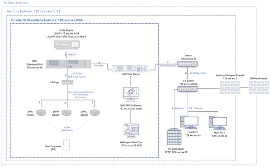
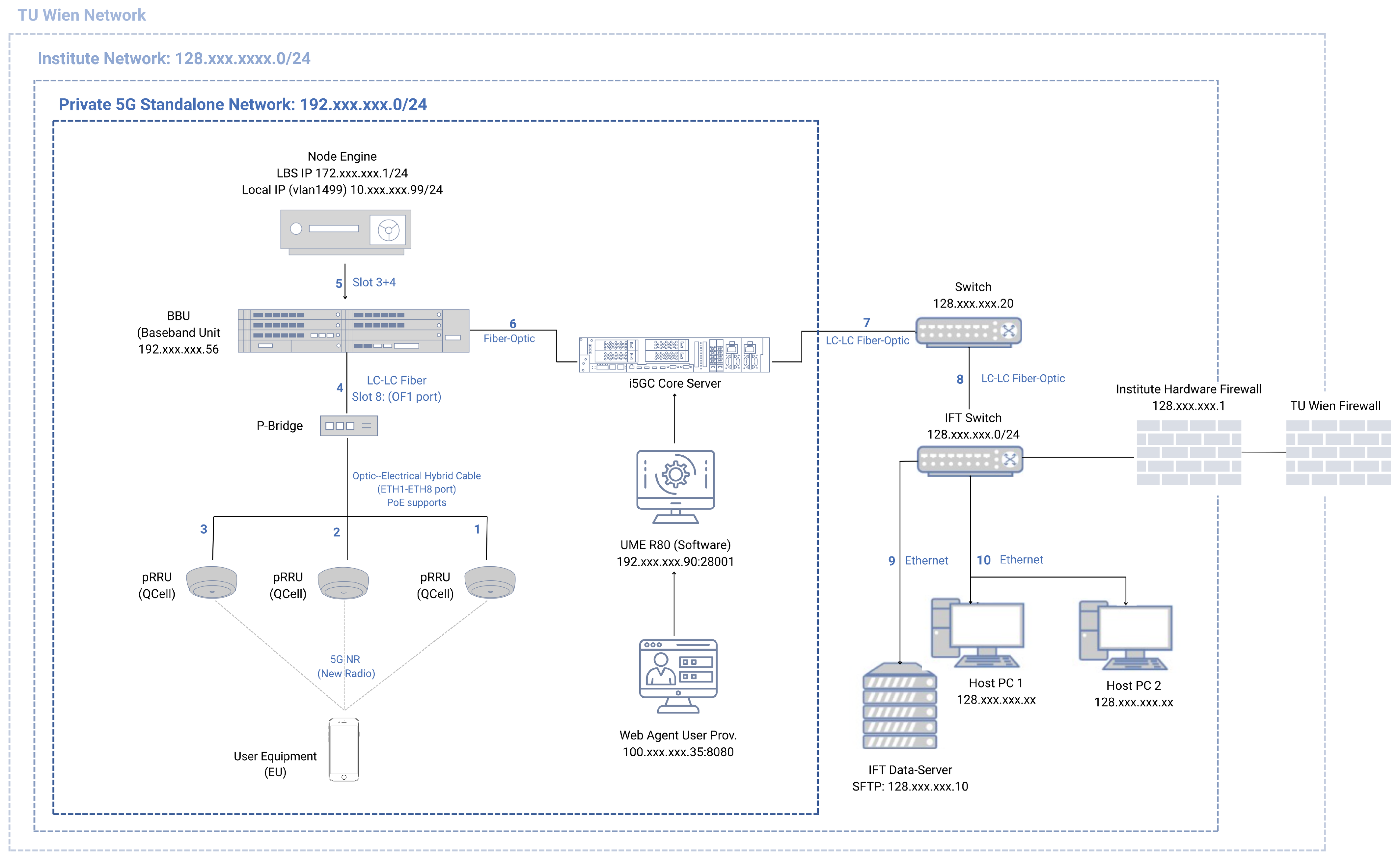
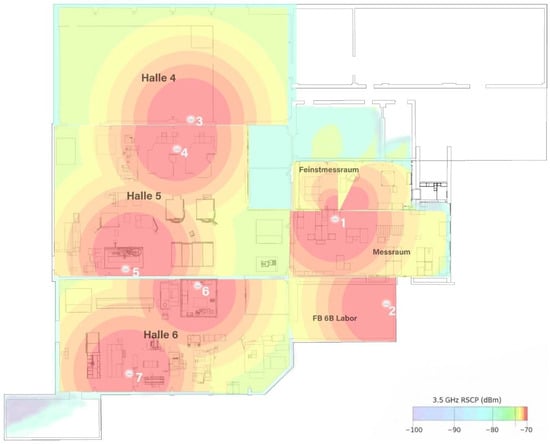
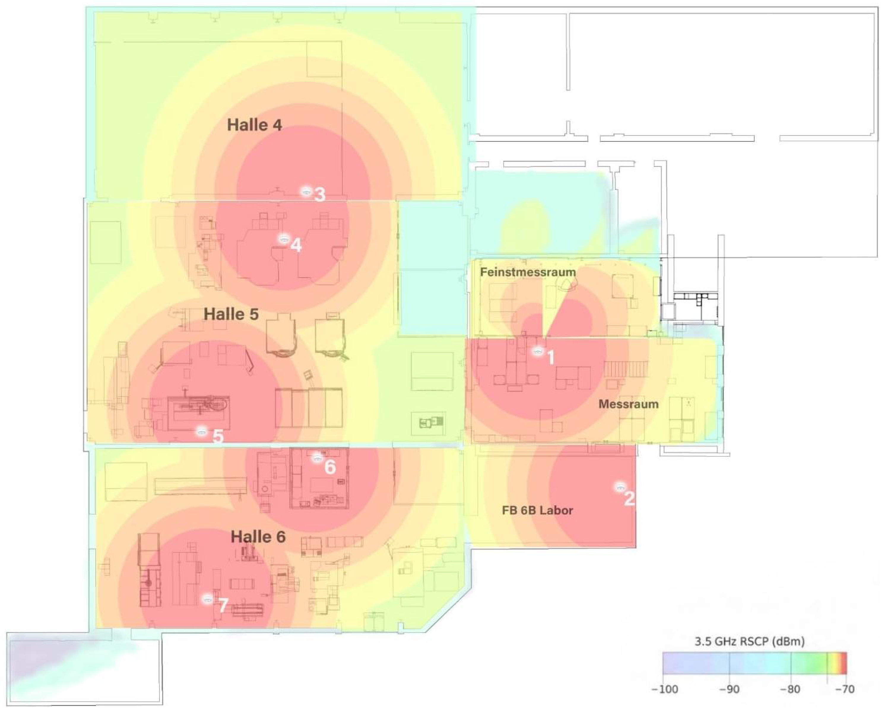
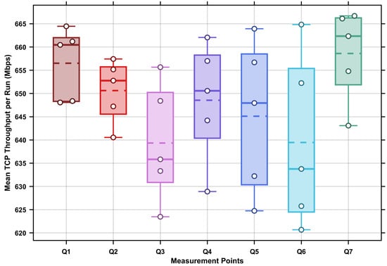
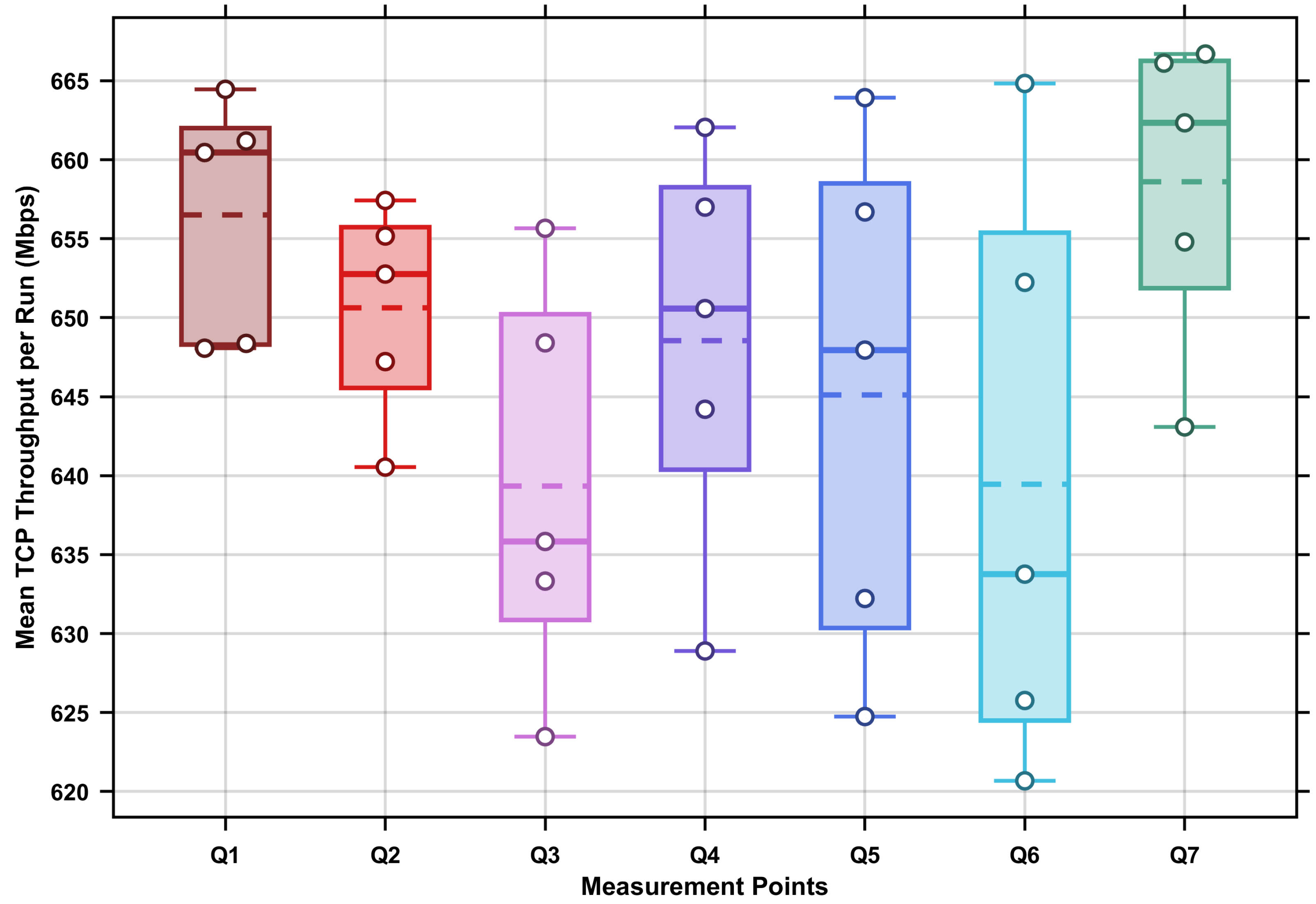
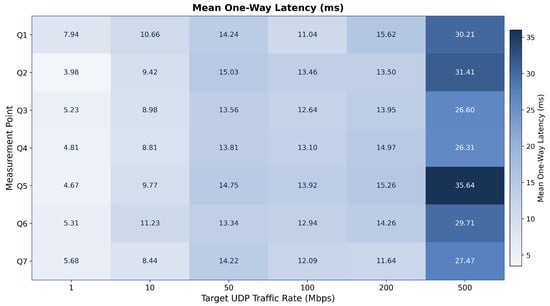
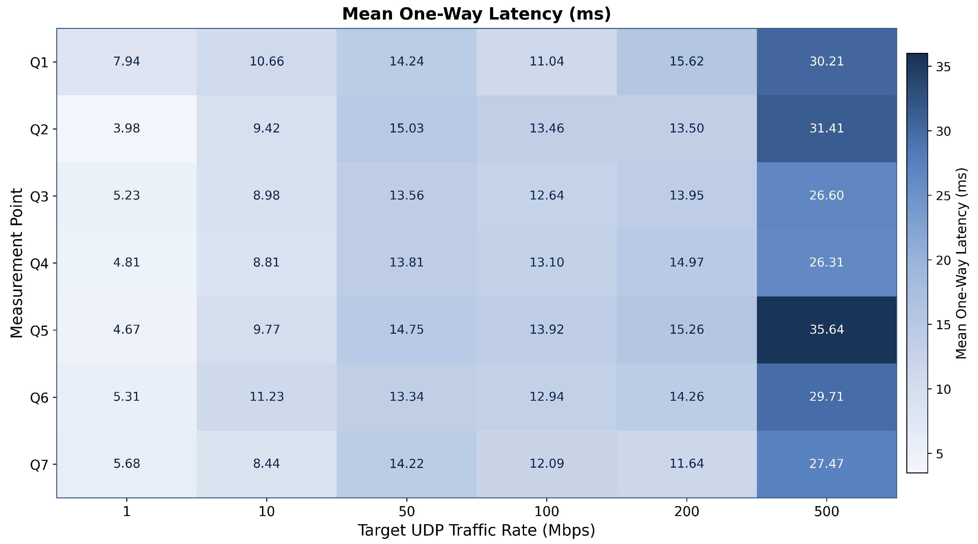
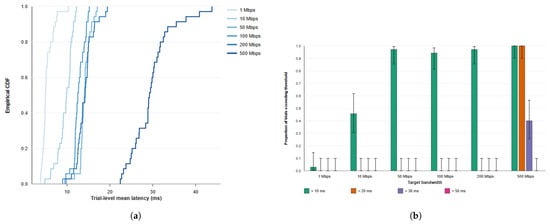
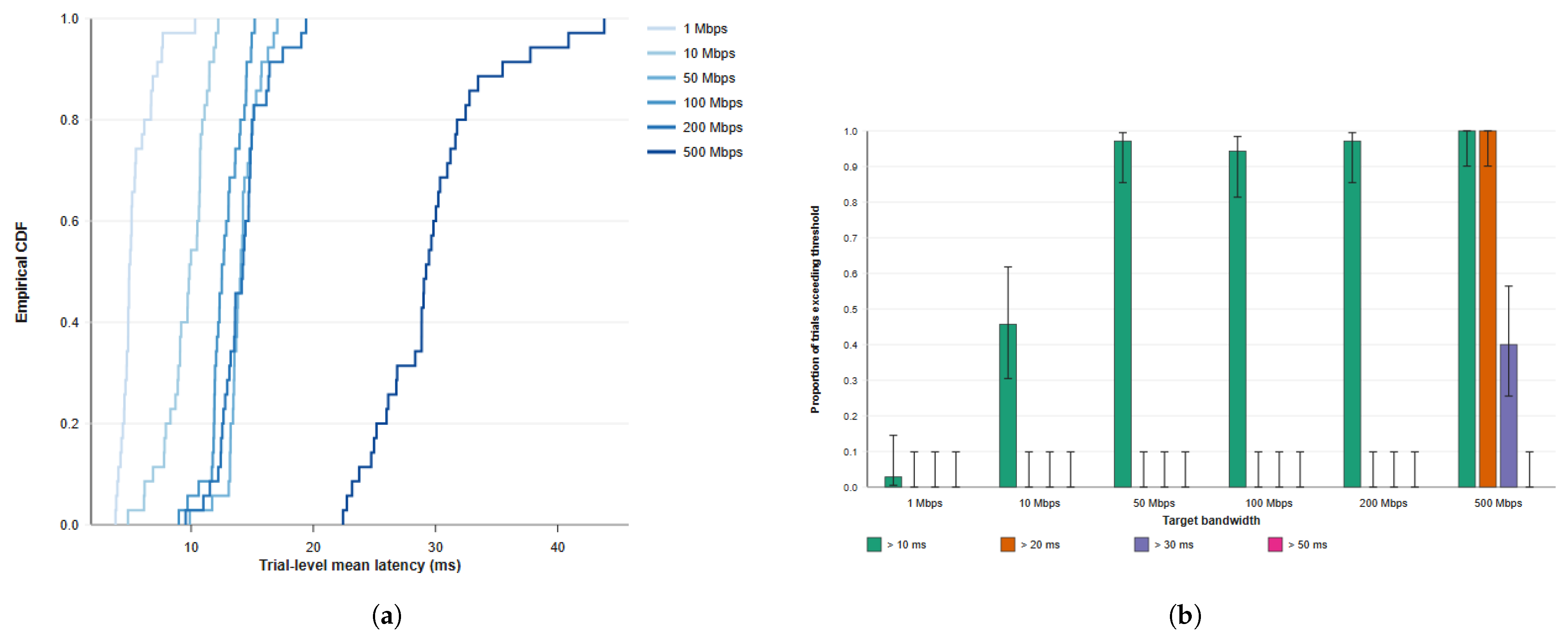
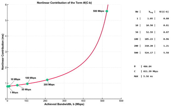
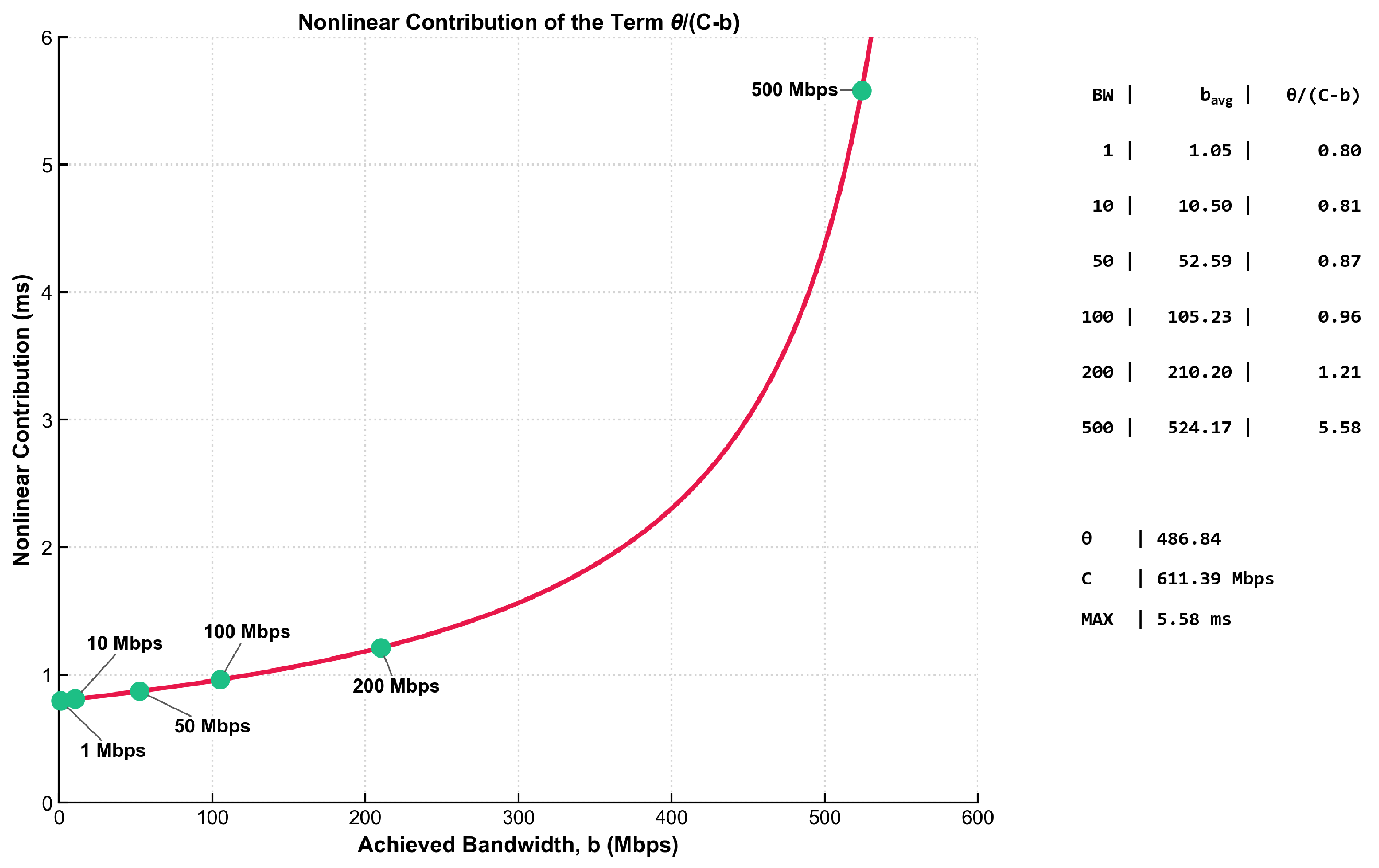
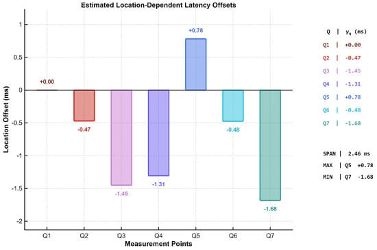
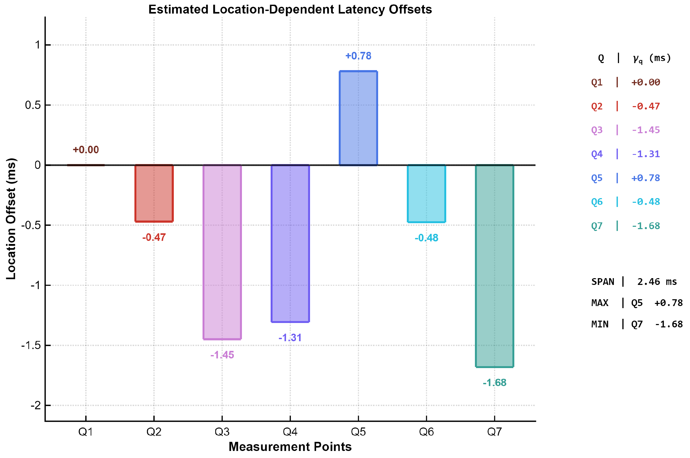
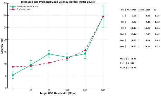
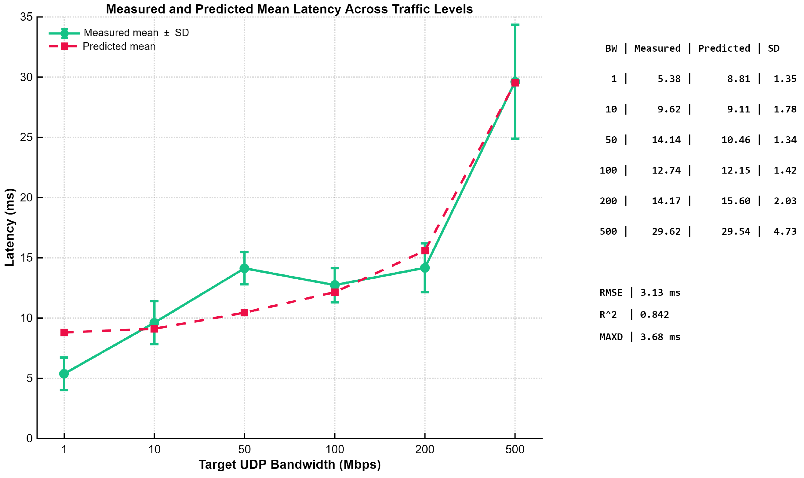

Disclaimer/Publisher’s Note: The statements, opinions and data contained in all publications are solely those of the individual author(s) and contributor(s) and not of MDPI and/or the editor(s). MDPI and/or the editor(s) disclaim responsibility for any injury to people or property resulting from any ideas, methods, instructions or products referred to in the content. |
© 2026 by the authors. Licensee MDPI, Basel, Switzerland. This article is an open access article distributed under the terms and conditions of the Creative Commons Attribution (CC BY) license.