


Abstract
Ferroresonance is a nonlinear phenomenon in power systems capable of producing irregular oscillations and severe overvoltages that threaten transformers, voltage transformers, cables, and associated equipment. This paper presents a structured comprehensive review of ferroresonance detection and mitigation techniques reported up to 2025, with particular emphasis on artificial intelligence (AI)-based approaches published during the last five years. A systematic literature search was conducted across IEEE Xplore, Scopus, Web of Science, and Google Scholar using predefined ferroresonance- and AI-related keywords. Eligible studies were screened using explicit inclusion criteria requiring demonstrated ferroresonance relevance. Numerical modeling approaches, electromagnetic transient tools, ferroresonance modes, and mitigation strategies are synthesized, followed by a critical evaluation of machine learning, deep learning, fuzzy logic, evolutionary algorithms, and hybrid intelligent frameworks. Particular emphasis is placed on signal preprocessing, data representation, real-time protection constraints, and cross-topology robustness. The review identifies key research gaps, including the scarcity of benchmark datasets, limited validation under realistic network variability, and the absence of standardized evaluation methodologies. While this work is presented as a structured comprehensive review, PRISMA-inspired screening principles were applied to enhance transparency and reproducibility. Current evidence indicates that hybrid approaches combining physics-informed preprocessing—particularly wavelet-based feature extraction—with lightweight neural classifiers offer the most practical pathway for relay-grade ferroresonance protection in modern smart grids.
1. Introduction
Ferroresonance is a nonlinear electrical phenomenon capable of producing severe and potentially damaging overvoltages. Ferroresonance can lead to severe voltage and current distortions that threaten power system reliability. It typically arises when a saturable inductance, such as a transformer, interacts with the system capacitance under specific conditions, including during switching operations or faults. The unpredictable behavior of ferroresonance produces complex system responses because its outcomes are difficult to control. The new analytical methods require complex modeling systems and detection technologies because they operate through distinct mechanisms from traditional methods.
The present-day power grid system is becoming increasingly susceptible to network failures because its evolving design introduces new points of vulnerability to ferroresonance. The implementation of Renewable Energy (RE) systems that use inverter-based distributed generation has led to different impedance patterns that modify power system and network resonance characteristics and has expanded the set of operating conditions under which ferroresonance may occur. Similarly, the proliferation of underground cables, lightly loaded lines, and capacitor-rich components has added operational difficulties for predicting and preventing ferroresonance events. Traditional analytical tools, though foundational, often fall short in capturing the nonlinear magnetization dynamics, hysteresis effects, and switching-induced transients that govern ferroresonant behavior. The system must operate effectively in both extensive power networks and in systems that undergo ongoing changes. In [1], ferroresonance was investigated in a distribution system integrated with multiple Distributed Generation (DG) and proposed an RLC shunt limiter as an effective mitigation technique.
The present Artificial Intelligence (AI) research has brought about fundamental changes, opening new possibilities for solving these problems. Machine Learning (ML), Deep Learning (DL), and hybrid intelligent systems have demonstrated strong potential in identifying early signatures of ferroresonance, extracting meaningful features from complex waveforms, and improving predictive capability under uncertainty. AI-enhanced methods enable users to monitor systems in real time while their protection systems adapt to changing system environments. The system uses advanced ML and data-driven classification methods, producing better results than conventional threshold-based and rule-based systems techniques. In addition, the deployment of AI-supported modeling frameworks improves nonlinear system modeling through their advanced capabilities. The system requires two operational functions to function properly: it must produce chaotic response patterns and exhibit transformer behavior to achieve optimal mitigation. Different mitigation strategies operate under different grid configurations. For instance, Ref. [2] introduced an algorithm that demonstrates the ability to detect faults using estimated flux analysis of voltage transformers. The study investigates the occurrence of ferroresonance oscillations that affect medium-voltage networks.
Modeling ferroresonance requires precise methods to characterize its behavior and to develop effective mitigation strategies. Traditional models fail to adequately represent the nonlinear dynamics involved. Recent research has used chaos theory to develop models of ferroresonance under nominal conditions, providing deeper insights into its unpredictable nature. These models allow users to create virtual scenarios, which enable them to develop improved design solutions for robust protection schemes.
Mitigation techniques for ferroresonance have evolved alongside advancements in detection and modeling. The system uses passive methods, including damping resistors and ferroresonance suppression circuits, which have been traditionally used. However, their effectiveness can be limited in complex systems. The effectiveness of damping devices in auxiliary power systems of high-voltage substations was analyzed in [3], emphasizing the importance of proper parameter coordination for successful mitigation. Active methods, including Static Var Compensators (SVCs), have also been explored for their ability to dynamically adjust system parameters to suppress ferroresonance.
The application of AI extends beyond detection to a mitigation phase. AI algorithms can predict which circumstances will produce specific results. The system will detect ferroresonance conditions and trigger automatic preventive measures to prevent these events. For example, morphological filtering techniques have been employed to remove high-frequency components from zero-sequence currents, thereby eliminating ferroresonance events.
The research shows promising results, but existing studies remain scattered across different fields. This includes diverse modeling methodologies, numerical simulation techniques, heuristic mitigation strategies, and a growing but heterogeneous body of AI-driven detection research. The evolution of power systems toward greater reliance on RE and automated control systems requires a new approach to power system protection.
This review addresses this gap by synthesizing recent advancements in ferroresonance detection and by focusing on emerging AI techniques during the last five years. The paper evaluates theoretical foundations, numerical approaches, electromagnetic transients (EMT) simulation tools, and contemporary mitigation strategies, while providing a comprehensive comparative analysis of AI methodologies, including neural networks, DL, fuzzy logic, evolutionary algorithms, and hybrid systems. By integrating insights from conventional engineering analysis and cutting-edge computational intelligence, this work aims to support researchers, utilities, and protection engineers in designing more resilient, adaptive, and predictive ferroresonance countermeasures suitable for next-generation smart grids.
2. Review Methodology
A structured literature search was conducted across IEEE Xplore, Scopus, Web of Science, and Google Scholar. The primary search string combined ferroresonance-specific and AI-specific keywords:
(“ferroresonance” OR “ferro-resonance” OR “VT ferroresonance”) AND (“artificial intelligence” OR “machine learning” OR “deep learning” OR “neural network”).
AI-assisted tools, SciSpace, were used in a limited capacity to support literature organization and preliminary screening. Illustrative screenshots of the search and screening interface are provided in the Supplementary Materials. All eligibility decisions, data interpretation, and technical synthesis were performed and verified by the authors to ensure methodological rigor and domain accuracy.
The review focuses on studies published between 2019 and 2025, while seminal earlier works were retained for foundational context.
Studies were included if they:
- Explicitly addressed ferroresonance phenomena.
- Presented detection, classification, modeling, or mitigation methods.
- Already peer-reviewed.
- Contained sufficient methodological detail.
On the other hand, studies were excluded if they:
- Addressed only general power system faults, without relevance to ferroresonance.
- Lacked technical validation.
- Duplicate or non-archival sources.
The initial search returned 861 papers, of which 681 were screened after deduplication, and 79 were finally included.
This work is presented as a structured, comprehensive review, rather than a full PRISMA systematic review, although PRISMA-inspired screening principles were applied. The study selection process followed PRISMA-inspired guidelines, and the detailed screening workflow is illustrated in Figure 1.
Figure 1.
PRISMA flow diagram of the literature screening and selection process.
3. Ferroresonance Phenomenon
Ferroresonance is a nonlinear electrical effect that happens when a saturable ferromagnetic inductor interacts with system capacitance during sinusoidal excitation. Its unusual harmonic levels and transient or steady-state overvoltages and overcurrents can pose significant risks to electrical devices [4,5]. It is often triggered by the interaction between nonlinear elements, such as transformers and capacitors, under specific operational conditions [5,6]. Linear resonance produces predictable steady-state responses, while ferroresonance can cause sustained overvoltages, subharmonic oscillations, and chaotic waveforms. This uncommon, nonlinear effect can also cause unknown malfunctions [7].
The physical mechanism of ferroresonance is strongly influenced by the nonlinear magnetization characteristics of transformer cores. When the core enters deep saturation, the effective inductance becomes state dependent, enabling energy exchange with network capacitances in a highly nonlinear manner. EMT studies have demonstrated that the phenomenon is sensitive to switching instant, remanent flux, system grounding configuration, and capacitive coupling, which together determine whether ferroresonance is initiated and which oscillatory regime emerges [8,9,10].
In dynamical systems, ferroresonance shows multi-stability. This means that, with the same system parameters, different steady-state responses can happen depending on the starting conditions. This feature explains why researchers have observed transitions between fundamental, subharmonic, quasi-periodic, and chaotic modes in the literature [4,11,12]. Because these modes can coexist, it is harder to predict and reliably detect them in real networks.
Unlike conventional short-circuit faults, ferroresonance waveforms typically contain rich spectral content extending beyond the fundamental frequency. Reported EMT and laboratory investigations frequently observe pronounced subharmonic components, intermittent chaotic bursts, and quasi-periodic voltage envelopes whose characteristics depend strongly on transformer magnetic behavior and network topology [13,14,15]. These features distinguish ferroresonance from many other power quality disturbances.
Unlike generic disturbance classification studies, this review focuses specifically on waveform characteristics driven by ferroresonance dynamics, as these signatures form the primary basis for data-driven detection methods.
In practical systems, ferroresonance events are complicated by measurement noise, switching transients, and load-induced harmonics. Field observations show substantial event-to-event variability even within the same substation, which reduces the effectiveness of fixed-threshold detection schemes and motivates the adoption of advanced signal processing and machine learning approaches [16,17,18].
Ferroresonance is a nonlinear phenomenon that can occur in different ways and depends on the system’s configuration. These factors make it hard to monitor and protect systems reliably. The signal-level implications of this variability are examined in Section 5.
3.1. Causes and Contributing Factors
Ferroresonance usually starts when system capacitance interacts with a saturable ferromagnetic inductance in conditions with little damping. Unlike typical disturbances, it is very sensitive to how the system is set up and switched, making its behavior irregular and hard to predict [19,20].
Several factors are known to increase the likelihood of ferroresonance. These include the presence of underground cables or grading capacitances, lightly loaded or unloaded voltage transformers, isolated or high-impedance grounding arrangements, and single-phase switching operations. The switching instant relative to the voltage waveform and the level of residual core flux can further influence whether the system enters a ferroresonant state [4].
In practical networks, these conditions may arise during routine operations such as feeder energization, transformer switching, or network reconfiguration. Because small variations in system parameters can shift the operating mode between fundamental, subharmonic, and chaotic regimes, deterministic threshold-based protection methods often struggle to provide reliable discrimination [8,9].
This strong dependence on initial conditions and network topology is a key reason why ferroresonance remains challenging to detect using conventional techniques and motivates the growing interest in advanced signal-processing and AI-based approaches discussed in later sections.
3.2. Nonlinear Magnetization Characteristic
Ferroresonance arises due to the nonlinear magnetization characteristics of ferromagnetic cores. Under typical conditions, the magnetizing branch of a transformer exhibits near-linear behavior. However, as the core approaches saturation, the magnetization curve demonstrates significant nonlinearity. In combination with system capacitance, this nonlinearity can result in multiple steady-state operating points.
The magnetizing inductance can be expressed in simplified form as a nonlinear flux–current relationship in Equation (1).
where is the magnetizing current and is the core flux. In the unsaturated region, is approximately linear, whereas near saturation it becomes highly nonlinear as depicted in Figure 2. This nonlinear characteristic is the fundamental mechanism enabling the multi-stable behavior observed in ferroresonance.
Figure 2.
Conceptual transformer hysteresis (B–H) curve relevant to ferroresonance analysis. Adapted from ref. [9].
From a modeling perspective, the magnetization curve is commonly represented using piecewise-linear, polynomial, or hysteresis-based formulations.
In practical systems, hysteresis further contributes to the energy exchange between the magnetic core and the surrounding electric network. Although detailed magnetic modeling can improve EMT accuracy, most ferroresonance studies focus primarily on capturing the saturation nonlinearity that governs the onset and modal behavior. As a result, ferroresonant voltage and current waveforms often exhibit significant distortion, intermittent bursts, and subharmonic content, motivating advanced signal-processing and AI-based detection approaches discussed in subsequent sections.
3.3. Resonance and Ferroresonance Distinction
It is important to distinguish ferroresonance from conventional linear resonance, as the two phenomena differ fundamentally in both mechanism and system response. Linear resonance occurs in networks composed of linear inductance and capacitance, producing a single predictable resonant frequency determined by circuit parameters. In its simplest form, the resonant frequency of a linear LC circuit is given in Equation (2).
where L and C represent the equivalent inductance and capacitance, respectively. Under linear conditions, the system response remains stable and uniquely defined for given parameters [21,22].
Ferroresonance, in contrast, happens when the inductive part of a system becomes magnetically saturated. When system capacitance interacts with a saturable ferromagnetic inductor, it creates strong nonlinearity, which means the system can settle into several different steady states. Because of this, the system might show fundamental, subharmonic, quasi-periodic, or even chaotic behavior, depending on the starting flux, the timing of switching, and the network’s layout [21]. Figure 3b shows a comparison between linear resonance and ferroresonance responses.
Figure 3.
Conceptual resonance slope illustrating nonlinear ferroresonance operating regions. Adapted from ref. [23]. (a) Conceptual graphical interpretation of voltage across a nonlinear inductor under ferroresonance conditions. (b) Resonance slope.
Unlike linear resonance, ferroresonance waveforms typically show severe distortion, irregular envelopes, and abrupt mode transitions that cannot be explained using linear phasor analysis. This nonlinear and multi-stable behavior significantly complicates detection and protection tasks, particularly in lightly damped or cable-rich networks [21]. Understanding this distinction provides the physical basis for the advanced signal-processing and AI-based detection techniques reviewed in the following sections.
4. Ferroresonance Modeling and Modes
Ferroresonance behavior has been extensively investigated using nonlinear equivalent circuit models and EMT simulation tools.
Ferroresonance can appear in multiple distinct operational configurations, determined by the structural organization of the network, the excitation parameters, and the initial magnetic flux conditions, with each configuration being defined by its distinctive waveform features and nonlinear dynamic behaviors.
4.1. Ferroresonance Modeling
Due to the phenomenon’s nonlinear and complex nature, modeling ferroresonance is challenging. Accurate modeling of ferroresonance is essential for predicting and mitigating its effects. Theoretical models are crucial to understanding and analyzing ferroresonance phenomena. These models help in designing effective mitigation strategies. A necessary element of the theoretical models is the detailed core model for step-down transformers, developed to investigate ferroresonance behavior. These models account for hysteresis, eddy current effects, and remnant flux, providing insights into the impact of passive and active suppression circuits [24]. Nonlinear inductance models are essential for analyzing ferroresonance in distribution networks. Nonlinear inductance models are used in voltage transformer (VT) to model nonlinear inductance. These models capture the dynamic behavior of VTs and their response to system disturbances. Dynamic models for ferroresonance are generalized, nonlinear inductance models aimed at studying ferroresonance in power networks, specifically 6–35 kV networks. These models provide accurate representations of ferroresonance modes, including fundamental frequency and subharmonic resonances [25].
Various modeling techniques have been developed to analyze and predict ferroresonance, each with strengths and limitations. The choice of modeling technique depends on the system’s complexity, the required level of accuracy, and the specific characteristics of the ferroresonant circuit. The following sections provide a detailed comparison of these modeling techniques, and a list of them is in Table 1.
Table 1.
Comparative analysis of modeling techniques used in ferroresonance studies.
4.1.1. Numerical Methods for Ferroresonance Modeling
Numerical methods use mathematical equations to describe how ferroresonant circuits work. They help explain the main mechanisms of ferroresonance, but they have limitations when modeling complex systems [19,39]. These methods can identify important parameters and show how they affect the system, but they usually work best for simple setups and are difficult to apply to real-world systems with complex nonlinear behavior.
Backward Differentiation Formula (BDF)/Numerical Differentiation Formula (NDF)
The Backward Differentiation Formula (BDF) and Numerical Differentiation Formula (NDF) are widely used for solving stiff differential equations arising in ferroresonance simulations. These methods are particularly effective at handling the stiffness inherent in transformer models. The NDF2 method, combined with the trapezoidal method, has been shown to suppress numerical oscillations and provide accurate results for voltage and current waveforms during both steady-state and transient ferroresonance [11].
Fractional-order models are often chosen over integer-order models because they describe capacitance and inductance more accurately. This results in a better understanding of how the system works [12,40].
The single-phase equivalent circuit is utilized for the analysis of series ferroresonance, comprising a series capacitance C and a nonlinear inductance L [23].
The numerical approach to solving the resonance expression when accounting for a nonlinear inductance is more intricate compared to finding a numerical solution for a straightforward RLC circuit. This is because the current depends on the magnetic flux (), which means that the saturation curve of the nonlinear inductance needs to be represented as a function of the magnetic flux. The saturation curve is normally represented as a polynomial Equation (3) [22,23].
The Equation (4) is a nonlinear second-order differential equation, and finding an analytical solution is quite intricate. In general, capacitance exhibits considerable sensitivity to ferroresonance [23].
A more detailed analytical framework is developed in [10] in which single-phase ferroresonant oscillations are represented by a nonlinear second-order differential equation. The model is solved over a range of excitation frequencies, including both the fundamental network frequency and subharmonic components.
Explicit Euler Method
The Explicit Euler method is a straightforward numerical integration technique used to solve differential equations describing ferroresonant circuits. This method is simple to implement but may require small time steps to maintain stability, especially when modeling nonlinear inductive elements with hysteresis [36]. Despite its simplicity, the explicit Euler method has been successfully applied to simulate ferroresonance modes in circuits with capacitive and inductive elements.
4.1.2. Numerical and Simulation-Based Models
The Electromagnetic Transients Program (EMTP) and PSCAD/EMTDC are powerful software tools for simulating ferroresonance in power systems. These tools are particularly useful for analyzing complex systems, such as three-phase transformers and distribution networks [16,17]. EMTP has been used to study the dynamics of ferroresonance in radial distribution systems and the impact of DG on the phenomenon [16].
Furthermore, time-domain simulation is a widely used method for analyzing ferroresonance. This approach involves solving the differential equations that describe the system’s behavior over time. Tools such as the Alternative Transients Program (ATP) are commonly used for this purpose [18,38]. It offers accurate modeling of nonlinear elements, including magnetic hysteresis and saturation. This makes it suitable for analyzing both transient and steady-state behavior. This comes at the expense of efficiency, as it is computationally intensive, especially for large-scale systems. This stems from the need for detailed models of system components, which can be challenging to obtain.
4.1.3. Nonlinear Electromagnetic (Magnetization) Models
Nonlinear dynamic analysis is a valuable tool for understanding the complex behavior of ferroresonant systems. It uses concepts such as phase portraits, Poincaré sections, and Lyapunov indices to analyze system dynamics [32,33]. This approach enables the identification of bifurcations and chaotic behavior, and facilitates examination of resonant conditions in the frequency domain. It is particularly useful for analyzing interactions between nonlinear inductance and capacitive elements [20,34].
It is difficult to apply to large-scale systems, and it requires advanced mathematical knowledge and computational tools, though. For instance, the Preisach theory is a physically correct hysteresis model that has been applied to ferroresonance modeling. This approach provides a precise representation of the hysteresis behavior of magnetic materials, making it suitable for studying the dynamic behavior of ferroresonant circuits [35]. The Preisach model has been shown to outperform the EMTP hysteretic model in terms of accuracy when simulating experimental results.
Improved models, such as the modified inverse Jiles-Atherton model, account for major and minor hysteresis loops, enhancing simulation accuracy. These models are crucial for predicting transient and steady-state ferroresonance behavior [32,36,41,42].
Ritz’s method of harmonic balance is an example of the frequency-domain analysis used to formulate closed-form solutions for ferroresonance problems. This method is particularly effective for fundamental-frequency ferroresonance and involves representing the transformer core’s magnetization characteristic using a polynomial [43]. The derived solutions enable the construction of stability maps that define the boundaries between safe and ferroresonant regions as functions of system parameters.
4.1.4. Tools for Ferroresonance Modeling and Analysis
Several tools support the analysis and simulation of power system dynamics, including ferroresonance. EMTP is widely used for simulating EMTs and is valued for its accurate modeling of nonlinear elements [14,18,38]. ATP offers a reliable alternative for transient simulations, especially in distribution systems [26,38]. Simulink provides a user-friendly interface, making it suitable for educational modeling and analysis of ferroresonance [18,27]. PSCAD/EMTDC is also commonly used for EMT analysis and excels at modeling complex nonlinear systems [29,41]. The latest version of ETAP integrates with PSCAD to enable both RMS and transient simulations.
Analytical models support conceptual understanding, whereas EMT-type simulations are the practical choice for system-level studies. Hysteresis-based magnetization models improve accuracy but increase computation time. Numerical stability analyses offer insight into chaotic and bifurcation behavior. A hybrid approach that combines detailed magnetic modeling with fast numerical solvers is the most effective strategy.
The selection of a modeling technique should match the system’s needs and the required accuracy. Future research should aim to improve modeling accuracy and efficiency, and to identify more effective methods to mitigate ferroresonance in power systems.
4.2. Ferroresonance Modes and Types
Ferroresonance can occur in several forms, each with distinct dynamic characteristics and system impacts. Understanding these modes supports effective detection and control. The most common is fundamental resonance, which arises when the resonant frequency of the nonlinear LC circuit matches the system’s main frequency [8,21,32]. This mode produces distorted but periodic waveforms that can persist if left unaddressed. It typically occurs during transformer energization or under light load conditions.
Subharmonic modes arise when the oscillation frequency becomes a fraction of the system’s fundamental frequency (e.g., 1/2, 1/3). These modes are often characterized by greater energy exchange between the inductive and capacitive components. Subharmonic behavior introduces severe waveform distortion and can evolve into chaotic resonance under certain conditions [21,33,36,41].
Multiple ferroresonance operating modes—including fundamental, subharmonic, and chaotic responses—have been analytically demonstrated using hysteresis-based transformer models, as reported in [44].
Chaotic ferroresonance exhibits non-periodic, unpredictable oscillations caused by nonlinear magnetic dynamics and hysteresis. This mode poses the greatest threat to system reliability, as protection systems often misinterpret chaotic waveforms, leading to false tripping or failure to operate. Chaotic resonance is difficult to predict and highly sensitive to switching conditions and remnant flux [8,21,44].
In the case of RLC circuits, ferroresonance can be divided into two main types: series ferroresonance and parallel ferroresonance [21]. An example of series ferroresonance occurs when a voltage transformer is energized through the grading capacitors of an open-circuit breaker, with the transformer placed between the phase and ground. Parallel ferroresonance can occur during a single phase to ground fault in an isolated neutral system, where inductance and capacitance are configured in parallel [21,23]. In addition to the series and parallel categories, ferroresonance can be classified as sustained or transient. Sustained ferroresonance behaves similarly to the second-order step response of an RLC circuit, in which a source provides the resonant effect, which can originate from the system’s voltage. This type of ferroresonance will persist indefinitely until the voltage source is disconnected. In contrast, transient ferroresonance diminishes over time because the source that supplies the resonant effect is a limited-energy source, such as the cable capacitance isolated from the network [21].
Transient ferroresonance occurs when the disturbance source is of limited duration or magnitude, resulting in oscillations that decay over time. Sustained ferroresonance persists indefinitely because of a continuous energy source, typically the system voltage or capacitor banks. Distinguishing between these behaviors is critical for designing mitigation strategies [4].
Series ferroresonance commonly arises when a transformer is energized through a capacitive element, creating a nonlinear series LC circuit. On the other hand, parallel ferroresonance occurs when inductive and capacitive elements are connected in parallel, often during ground faults in isolated or resonant-grounded systems. Understanding these configurations helps engineers identify vulnerable topologies [4].
5. Ferroresonance Data Characteristics
AI-driven ferroresonance identification is complicated by the phenomenon’s inherent electromagnetic nonlinearity and its marked dependence on prevailing system conditions. Unlike conventional short-circuit faults, ferroresonance is governed by the interaction between a saturable magnetic inductance and network capacitance, which can produce multiple steady-state solutions, bifurcations, and chaotic responses under identical system parameters [21,39]. Extensive EMT studies have shown that the resulting waveforms are highly sensitive to initial flux conditions, switching instants, and network topology, making deterministic pattern recognition significantly more difficult [8,22].
From a signal-analysis perspective, ferroresonance events typically exhibit the following distinguishing characteristics:
- Strong nonlinearity arising from core saturation.
- Multi-stable operating regions with abrupt mode transitions.
- Chaotic and quasi-periodic regimes under certain parameter ranges.
- Pronounced sensitivity to switching instant and remanent flux.
- Topology-dependent modal behavior influenced by grounding and cable capacitance.
Unlike conventional short-circuit disturbances, ferroresonance waveforms frequently contain rich spectral content extending beyond the fundamental frequency. Reported EMT and laboratory investigations consistently observe [11,13]:
- Pronounced subharmonic components (e.g., 1/2, 1/3, and fractional harmonics).
- Quasi-periodic voltage envelopes.
- Intermittent chaotic bursts with broadband spectra.
- Waveform distortion strongly coupled to VT core magnetization characteristics.
A significant real-world characteristic is the variability in behavior across individual events within the same network. Minor changes in factors such as residual flux, the angle at which breakers close, or system capacitance can cause the system to transition among fundamental, subharmonic, and chaotic ferroresonance states [12,18]. This inconsistency undermines detection methods that rely solely on threshold values and supports the adoption of data-driven techniques that can account for nonlinear dynamics.
Additional measurements indicate that ferroresonance waveforms are commonly corrupted by environmental noise, transients from switching events, and load harmonic distortion [32,41]. As a result, reliable feature extraction must simultaneously provide precise time localization, clear spectral separation, and noise-rejection capabilities. Time–frequency decomposition methods—wavelet techniques in particular—have proven more effective at extracting ferroresonance patterns than purely time-based statistical measures [26,30].
Collectively, these attributes explain both the widespread preference for sophisticated machine learning and signal processing tools for identifying ferroresonance and the ongoing challenges of ensuring that models generalize well and perform robustly across different system configurations.
The unique characteristics of these signals necessitate specialized preprocessing to extract robust, discriminative features for AI-driven detection systems.
6. Signal Preprocessing for AI-Based Detection
Preprocessing of input signals is an essential step in ML-based ferroresonance detection systems. Since ferroresonance waveforms exhibit significant nonlinear behavior, non-stationary properties, and are frequently corrupted by transient switching events and harmonic background interference, effective signal preparation and feature formulation are necessary to achieve consistent model accuracy. The sections that follow discuss key preprocessing methodologies reported in the academic literature, covering data collection considerations, joint time-frequency transformations, self-adjusting decomposition algorithms, and complementary strategies for reliable ML applications.
The surveyed literature consistently demonstrates that raw waveform input rarely provides sufficient discriminative power for reliable ferroresonance detection, particularly under noisy operating conditions and across varying network topologies. Practical detection pipelines, therefore, rely on preprocessing to [24,31]:
- Isolate informative components (subharmonics, interharmonics, chaotic signatures).
- Improve robustness to noise and switching transients.
- Produce feature representations compatible with classical ML or DL models.
6.1. Practical Acquisition and Conditioning
In relay and monitoring applications, preprocessing begins with robust signal conditioning. The selection of the sampling rate is critical and depends on the application. Sampling frequencies between 2–10 kHz are typically adequate for recording subharmonic frequencies and transient development. However, a more detailed analysis of transient characteristics may require sampling frequencies of 20 kHz or higher, depending on the specific measurement equipment used [33,40]. Anti-aliasing and filtering are typically applied where necessary, with notch filtering for persistent interference. Caution must be exercised to prevent the attenuation of subharmonic frequencies that are typical indicators of ferroresonance [34]. Segmentation/event detection is another stage typically found in relay systems. Their techniques rely on switching occurrences, root-mean-square variations, or change-point identification, which are commonly employed to distinguish between initiation phases and developmental periods. Dynamic segmentation methods enhance the ability to detect early-stage emergence and shifts between operational modes [37,42]. Normalization, in which per-window scaling (z-score, min–max, or per-phase normalization) is applied, improves cross-case comparability and stabilizes learning, especially under varying VT ratios and measurement gains. This practice appears to be necessary for ferroresonance detection [44].
These steps are particularly important because ferroresonance signatures can be masked by switching transients and background harmonics, and because event-to-event variability makes fixed thresholds unreliable.
6.2. Discrete Wavelet Transform (DWT)
Discrete Wavelet Transform (DWT) remains one of the most widely adopted techniques because it:
- Isolates subharmonic energy bands;
- Provides excellent time localization;
- It is computationally compatible with relay implementation;
- Exhibits strong noise robustness.
Wavelet-energy features (e.g., band energies, entropy measures, coefficient statistics) have repeatedly been shown to be sensitive to early ferroresonance onset and to discriminate between fundamental, subharmonic, and chaotic modes when appropriately selected [45,46]. In practice, compact feature sets derived from a small number of decomposition levels are preferred for relay-grade latency constraints.
6.3. Wavelet Scalograms and Time–Frequency Images for Convolutional Neural Networks (CNN) Input
For DL approaches, voltage or current signals are commonly converted into time–frequency images using Continuous Wavelet Transform (CWT) scalograms, Short-Time Fourier Transform (STFT) spectrograms, or synchrosqueezed transforms for enhanced frequency localization [47,48,49].
Convolutional Neural Network (CNN)-based ferroresonance detection generally requires a signal-to-image transformation stage; direct input of raw waveforms rarely achieves comparable performance with limited datasets [47,50]. Recommended practices include consistent color map scaling (or a fixed dynamic range), standardized window lengths, and careful avoidance of information leakage when windows overlap.
6.4. Variational Mode Decomposition (VMD)
Recent studies indicate that Variational Mode Decomposition (VMD) provides improved modal separation, enhanced robustness under noisy conditions, and superior handling of chaotic ferroresonance regimes. VMD is particularly effective when ferroresonance signatures overlap with nonstationary switching artifacts. Typical pipelines extract intrinsic mode function-like modes and compute energy/entropy descriptors or feed modal components into lightweight classifiers. The primary limitation remains increased computational burden relative to DWT; thus, practical use often limits the number of modes and iterations [51,52,53].
6.5. Short-Time Fourier Transform (STFT)
STFT is useful for fundamental versus subharmonic discrimination, quasi-steady ferroresonance analysis, and rapid spectral screening in monitoring applications. However, the fixed window length constrains performance during fast transient evolution. Multi-resolution approaches (e.g., wavelets) typically outperform STFT in onset detection, whereas STFT can remain competitive for steady regimes when parameterized appropriately [54,55,56].
6.6. Additional Preprocessing Techniques
Denoising improves robustness under field conditions. Common approaches include wavelet thresholding, median filtering, and robust smoothing. Care must be taken not to remove informative subharmonic content; therefore, adaptive denoising tuned to preserve low-frequency components is preferred [57,58,59].
Some models, including Support Vector Machine (SVM), decision trees, or lightweight Artificial Neural Network (ANN) models, typically combine effective features. Time-domain descriptors (RMS, crest factor, zero-crossing irregularity), frequency-domain descriptors (subharmonic ratios, spectral flatness), and time–frequency descriptors (wavelet energies, entropies) provide distinct dimensions for assessing waveform performance. Hybrid feature sets consistently outperform single-domain approaches, particularly for discriminating chaotic ferroresonance [60,61].
Because ferroresonance datasets are often small and imbalanced, augmentation is frequently employed, including additive noise consistent with measurement chains, random amplitude scaling, and time shifts that preserve physical plausibility [62]. For imbalanced classes, cost-sensitive learning, resampling, and calibrated decision thresholds are preferred over naive oversampling, which can inflate performance estimates [63].
7. Artificial Intelligence Techniques
Expanding on the preprocessed representations delineated in Section 6, a wide range of AI techniques have been meticulously examined for detecting ferroresonance in contemporary power systems. Due to ferroresonance’s complex characteristics—including significant nonlinearity, multiple stable states, and occasional chaotic behavior—traditional threshold-based or rule-driven techniques frequently demonstrate insufficient reliability across different network scenarios. As a result, researchers have investigated data-driven methods to improve detection accuracy and flexibility. Unlike generic disturbance classification studies, the following discussion focuses specifically on ferroresonance-driven waveform characteristics and protection requirements.
The AI approaches are organized by learning method and design features into three categories: classical machine learning techniques, such as SVM, decision trees, and fuzzy systems; DL models, including CNN and RNN/LSTM; and hybrid or optimization-assisted frameworks, such as Genetic Algorithm (GA)-tuned models and ensemble methods. This classification clarifies how these models are developed and applied in ferroresonance detection studies.
7.1. Machine Learning (ML)
ML encompasses algorithms that learn input-to-output mappings or discover structure from data rather than following fixed, pre-programmed rules. ML includes supervised learning (learning from labeled examples), unsupervised learning (finding patterns in unlabeled data), and reinforcement learning (learning through interaction and rewards) [50,51].
ML algorithms process features extracted from voltage and current waveforms, protection relay signals, and system measurements to classify fault types, predict equipment failures, and support protective decision-making [50,51].
A large portion of published studies relies primarily on EMT simulation datasets (EMTP/PSCAD), with limited availability of hardware-in-the-loop or utility field measurements.
7.2. Deep Learning (DL)
DL refers to multi-layer (deep) neural network architectures that automatically learn hierarchical feature representations from raw signals such as time series, images, or spectrograms. Unlike traditional ML that requires manual feature engineering, DL methods learn features automatically from data, though they typically require large labeled datasets for effective training [50,51].
DL excels at processing raw waveform data, automatically extracting relevant features without manual signal processing, making it particularly valuable for complex phenomena like ferroresonance where feature engineering is difficult [52,53].
7.3. Artificial Neural Networks (ANNs)
ANNs are computational models inspired by biological neural networks particularly for modeling nonlinear ferroresonance waveforms in protection applications, consisting of interconnected layers of nodes (neurons) with weighted connections. Common architectures include Multi-Layer Perceptrons (MLPs), CNNs, and Recurrent Neural Networks (RNNs). ANNs are trained through optimization algorithms (typically backpropagation) to approximate complex nonlinear functions, making them suitable for both classification and regression tasks in power system protection [51,54,64].
ANNs are widely used for fault classification, protective relay decision-making, and pattern recognition in power system signals due to their universal approximation capability and ability to learn from historical data [51,54,55].
7.4. Support Vector Machines (SVMs)
SVMs are margin-based supervised learning algorithms that find optimal hyperplanes to separate different classes in feature space. SVMs can handle nonlinear classification using kernel functions (e.g., Radial Basis Function (RBF) or polynomial) that implicitly map inputs to higher-dimensional spaces. SVMs are particularly effective with moderate-sized feature sets and are relatively robust to overfitting compared to some other methods. SVMs have been successfully applied to fault type classification, fault location, and protection zone identification, particularly when working with carefully engineered features from time-domain or frequency-domain signal analysis [51,65,66].
7.5. Decision Trees and Ensemble Methods
Decision trees use if–then rules to split data into different regions. Each internal node checks a feature, branches show possible outcomes, and leaf nodes give class labels or regression values. Ensemble methods like Random Forests combine several decision trees to boost prediction accuracy and help prevent overfitting. These approaches make it easier to understand the rules and analyze which features matter most. In power systems, decision trees are useful because they are easy to understand, run quickly, and can handle both numerical and categorical data. They are especially important when explaining protection decisions [51,66].
7.6. Fuzzy Logic
Fuzzy logic is a reasoning framework that handles uncertainty and imprecision by allowing variables to have degrees of membership in sets rather than binary (true/false) membership. Fuzzy systems use linguistic rules (e.g., “IF voltage is high AND current is medium THEN fault is likely”) that mimic human expert reasoning. Fuzzy inference systems combine multiple fuzzy rules to make decisions under uncertainty [51,67].
Fuzzy logic is particularly valuable in power system protection for handling uncertain measurements, noisy signals, or situations where exact thresholds are difficult to define. It enables robust decision-making under imprecision [51,54,67].
7.7. Genetic Algorithms (GAs) and Evolutionary Methods
GAs are population-based optimization techniques inspired by biological evolution. They maintain a population of candidate solutions and iteratively improve them via selection, crossover (recombination), and mutation. GAs are used for parameter tuning, feature selection, hyperparameter optimization, and solving complex optimization problems where gradient-based methods are unsuitable. In power system applications, GAs are commonly used to optimize neural network architectures, select optimal feature subsets, tune protection relay settings, and optimize power system controller parameters [50,68].
7.8. Expert Systems
Expert systems are knowledge-based systems that encode domain expertise as if–then rules and use inference engines for diagnostic or decision-making tasks. Traditional expert systems depend on knowledge engineering, which involves extracting and formalizing expert knowledge. Although once essential for power system protection, expert systems are now less common in recent literature due to challenges in knowledge acquisition and maintenance.
Expert systems were among the first AI applications in power systems, used for fault diagnosis, alarm processing, and protection coordination. Modern approaches often combine expert rules with machine learning for improved adaptability [51,69].
7.9. Comparative Analysis of AI Techniques
Each of the above-discussed AI techniques offers distinct strengths in modeling complexity, interpretability, and computational demand. A synthesis of comparative findings across performance, robustness, and implementation dimensions highlights the varying suitability of these techniques for different protection contexts. Table 2 lists strengths and weaknesses of these AI techniques for ferroresonance detection application. A common challenge across AI-based ferroresonance detectors is maintaining robust performance under varying network configurations and limited availability of labeled field data.
Table 2.
Strengths and limitations of AI techniques specifically reported for ferroresonance detection applications.
Also, Table 3 presents a quantitative comparison of the listed AI approaches across key performance dimensions. The qualitative ratings are gathered from literature reviews. These ratings offer a comparative qualitative overview rather than a strict quantitative benchmark, as the underlying studies employ heterogeneous datasets and varying evaluation conditions.
Table 3.
Comparative assessment of AI techniques for ferroresonance detection considering accuracy, computational burden, and relay suitability.
The performance ranges reported in Table 3 are directly synthesized from the cited ferroresonance-focused studies referenced in the table. Because the underlying works employ different datasets, network configurations, and evaluation protocols, the reported values are not statistically aggregated but instead reflect representative ranges observed in the literature. The Table is intended to provide comparative qualitative insight into relative method performance rather than strict quantitative benchmarking.
ANNs, including multilayer perceptrons and their DL extensions, have been widely studied for modeling complex transient behaviors. Their capacity for universal function approximation and rapid inference makes them strong candidates for high-speed protection schemes [56,57]. DL architectures such as CNNs and Long Short-Term Memory (LSTM) networks further enhance these capabilities by automating feature extraction and capturing temporal patterns. Their demonstrated high accuracy in classifying disturbance signatures has positioned them at the forefront of ferroresonance detection research [59,60]. However, these methods suffer from well-documented limitations, including extensive data requirements, high training costs, and limited interpretability, which constrain their deployment in environments where transparency and auditability are essential [59,60,62].
Rule-based systems, such as fuzzy logic frameworks and expert systems, are valued for their clarity and reliability when working with uncertain or incomplete data. Fuzzy logic systems use clear language rules and membership structures, so domain experts can check results and trust the system’s decisions [70]. Expert systems offer transparent reasoning but cannot learn from new data, which makes it hard for them to adapt to changes in the grid [70]. Hybrid neuro-fuzzy systems bring together the accuracy of fuzzy logic and the flexibility of neural networks. This approach can improve accuracy and keep some interpretability, but as the system gets more complex, it can become harder to understand because there are more rules [62].
Margin-based and tree-based methods balance interpretability and predictive performance. SVMs generalize well with limited data and excel in high-dimensional spaces, but their performance depends on kernel selection and training time increases with larger datasets [61]. Decision trees provide transparent, hierarchical rules and fast inference, making them suitable for real-time protection. Random forests address overfitting by using ensemble averaging to enhance robustness and accuracy. These ensembles, including boosting-based techniques, deliver high detection performance, especially with imbalanced or noisy data, though they reduce interpretability and require greater computational resources [61,70].
Comparative analyses across performance metrics further underscore these distinctions. DL and ensemble methods generally yield the highest classification accuracies [59,60], while logic-based systems provide the greatest interpretability. Inference time is critical for sub-cycle protection, favoring ANNs, fuzzy logic systems, expert systems, and decision trees, all of which achieve millisecond-scale response times. Data requirements vary dramatically across methods, with DL models requiring orders of magnitude more training data than SVMs, decision trees, or transfer learning-based approaches. Complexity profiles follow similar patterns, with deep models exhibiting the highest architectural and computational demands [56,57,61,70].
Interpretability remains a central concern in the application of AI to protection systems, where operators and regulators require transparent justification for automated decisions. Fuzzy logic, expert systems, and decision trees offer the clearest reasoning mechanisms [61,70], while neural networks and DL architectures rely on post hoc explainability tools such as saliency maps and relevance propagation [56,57,59,60]. Although these techniques improve comprehension, they do not fully resolve the models’ intrinsic opacity. This limitation has implications for regulatory compliance and operator trust, particularly in high-stakes applications such as ferroresonance mitigation.
Studies of various power system tasks show that no single AI method performs best across all applications. Techniques with strong nonlinear modeling, like DL, neuro-fuzzy systems, and ensembles, are most useful for detecting ferroresonance, where it is important to identify complex modal interactions. Faster, more interpretable methods, such as artificial neural networks, fuzzy systems, and decision trees, are better suited for real-time protection. Table 4 gives an overview of AI tools used in power system protection, including for ferroresonance detection.
Table 4.
Application suitability matrix for AI techniques in ferroresonance protection.
Implementation considerations highlight several trade-offs. DL and ensemble models have high development and deployment costs due to computational demands [59,61,62]. In contrast, decision trees, SVMs, and ANNs are more cost-effective [56,61,70]. Expert systems are easy to deploy but require significant ongoing maintenance as system conditions evolve [70]. DL, random forests, and ensembles perform well with large-scale or diverse data, while fuzzy logic and decision trees are effective in noisy or incomplete data environments. Transfer learning is useful when training data is limited, though it poses risks if there is a domain mismatch [62,70].
Because the reported metrics originate from heterogeneous test systems and datasets, the comparisons in Table 3 and Table 4 should be interpreted as qualitative performance trends rather than strict quantitative benchmarks.
Based on comparative criteria, the MLP combined with DWT is a highly practical candidate for real-time ferroresonance detection, with respect to accuracy, inference time, hardware feasibility, and stability. The ANN technique provides sub-millisecond inference (ideal for real-time relays), effectively models ferroresonance signatures, and has moderate data requirements (1k–10k samples), thereby making it trainable even with limited ferroresonance data. On the other hand, wavelet preprocessing significantly improves reliability, reduces noise sensitivity, and extracts modal energy components that are crucial for identifying the initiation of ferroresonance. This combination has already been shown in practice for detecting voltage transformer ferroresonance and transformer differential anomalies.
8. Sensitivity to Network Configuration
AI-based ferroresonance detection methods reported in the literature generally demonstrate high accuracy under the specific conditions for which they are trained and validated. However, ferroresonance behavior is inherently sensitive to system configuration and operating conditions, raising important questions regarding model generalization and field robustness [10,29,38,39]. This sensitivity is a well-known characteristic of nonlinear ferroresonant systems and must be explicitly considered when evaluating AI model portability.
From a physical perspective, the initiation and dynamic properties of ferroresonance are markedly influenced by various network parameters, including grounding configurations, cable and line capacitance, the magnetic properties inherent in VT, switching angles, remanent flux, system loading, and the network topology [18,32,41].
While such studies provide substantial evidence of concept validation, they may not fully represent the variability of real-world conditions encountered within operational power systems [59,72].
Furthermore, only a minor fraction of the academic literature incorporates validation through hardware-in-the-loop (HIL) systems or empirical utility field measurements, both of which are crucial for assessing deployment readiness [65,66,71].
To enhance practical reliability, future research should prioritize the development of multi-topology training datasets, systematic parameter-sensitivity studies, and cross-system validation protocols. Physics-informed feature design and hybrid modeling–learning frameworks may also improve robustness by embedding known ferroresonance dynamics into the learning process. In addition, uncertainty quantification and explainable AI techniques should be incorporated to support protection-engineering confidence [66,71].
Overall, while AI-assisted ferroresonance detection has shown significant promise, sensitivity to network configuration remains a key barrier to widespread field deployment and represents a high-priority direction for future investigation.
9. Artificial Neural Networks for Ferroresonance Detection
Owing to the extensive body of work and practical relevance of ANN-based approaches in ferroresonance detection, they are discussed in detail. ANNs have become indispensable tools in modern power system protection, offering powerful pattern recognition and nonlinear function approximation capabilities. Neural networks were inspired by biological neural systems and have evolved through multiple generations from simple perceptrons in the 1950s to modern DL architectures. In power systems, ANNs have been applied since the 1990s for fault detection, classification, and protection [73,74]. The evolution from shallow to deep architectures, combined with advances in optimization algorithms and computational power, has dramatically expanded ANN capabilities for complex power system applications [58,63]. Backpropagation is the main algorithm for computing gradients of the loss function with respect to network parameters. It uses the chain rule to efficiently send error signals backward through the network layers [58,74]. In ferroresonance applications, ANN models are primarily employed to classify nonlinear voltage waveform patterns derived from time–frequency preprocessing.
Early studies showed that shallow neural networks, such as MLPs, can detect nonlinear behavior in voltage transformers when using features selected by experts [56]. This supports the strengths listed for MLPs in Table 5, which highlights their low computational needs and real-time suitability. RBF networks also train quickly and are easier to interpret, but they struggle to model highly irregular resonant waveforms. Recurrent networks are better at following changes in ferroresonant oscillations over time, as recent power system monitoring studies have shown [73]. These findings are consistent with Table 5, which rates RNN-based models highly for analyzing sequential waveforms.
Table 5.
Strengths and weaknesses of major ANN architectures.
9.1. Comparative Analysis of ANN Architectures
ANN architectures vary in accuracy, training speed, and inference speed, making some more suitable for specific applications. Shallow models such as MLPs and RBFs train and run quickly with moderate data, making them ideal when speed and efficiency are priorities. Convolutional networks and RNNs offer higher pattern recognition accuracy with spatial or temporal data but require more data, longer training times, and often Graphics Processing Unit (GPU) support. Hybrid CNN–RNN models achieve the highest accuracy by combining both learning types, but they demand even more data, train slowly, and are less interpretable. Generally, detecting raw ferroresonance voltage waveforms does not apply directly to CNNs. Instead, signals are converted into time–frequency representations, such as continuous wavelet transform scalograms or STFT spectrograms. These representations reveal spectral features associated with subharmonic and chaotic ferroresonance. This approach is effective because ferroresonance is nonstationary, and image-based data facilitates feature extraction compared to time-domain data. Ensemble methods enhance accuracy and robustness by combining multiple models, though this increases complexity and slows inference. Ultimately, selecting a model for ferroresonance detection requires balancing accuracy, efficiency, and transparency.
Table 6 provides a comprehensive performance comparison of major ANN architectures across key metrics, including accuracy, training speed, inference speed, data requirements, and interpretability. This comparison guides architecture selection based on specific application requirements.
Table 6.
Performance comparison of major ANN architectures.
9.1.1. Application Suitability
Various ANN architectures are best suited for different power system tasks, such as real-time protection, waveform analysis, sequential processing, and ferroresonance detection. Shallow architectures such as MLPs and RBFs work well for fast, real-time protection and waveform analysis because they offer low latency and stable results. RNNs, including LSTM and GRU networks, perform better on sequential and time-based tasks because they can track changes over time, but they require more computing power. Hybrid CNN-RNN models combine spatial and temporal features, making them especially useful for detecting ferroresonance, which involves complex dynamics. Ensemble methods are reliable across many applications, showing strong robustness and the ability to generalize.
Task-specific suitability analysis in Table 7 reinforces these conclusions: models with strong temporal representation capabilities are best aligned with ferroresonance detection, while shallow ANNs remain appropriate for simpler real-time monitoring tasks. These observations are consistent with recent system-level assessments of ferroresonance mitigation strategies, which increasingly favor hybrid architectures that fuse modal decomposition with adaptive neural inference. It is worth noting that the qualitative ratings in the suitability matrices (e.g., Excellent, Good, Fair, Poor) are based on collective evidence from the reviewed literature. The assessment considers factors such as detection accuracy, robustness to waveform variability, computational complexity, and applicability to ferroresonance scenarios. These ratings provide a comparative qualitative overview rather than strict quantitative benchmarking, since the underlying studies use heterogeneous datasets and evaluation conditions.
Table 7.
Application suitability matrix for ANN architectures.
9.1.2. Computational Requirements
When deploying algorithms, it is important to consider computational limits, as these affect which methods can be used. Lightweight models such as MLPs and RBF networks require little computational power and memory. This makes them suitable for real-time use on standard Central Processing Unit (CPU) and easy to add to embedded protection devices. On the other hand, DL models such as CNNs and RNNs need much more computing and memory, especially during training, which usually requires GPU acceleration. Although inference can be improved with edge accelerators such as Tensor Processing Units (TPUs), using these models in embedded systems is often limited by hardware costs and power consumption. Hybrid CNN-RNN and ensemble methods also impose additional computational demands, so they are mostly used for offline analysis or in central monitoring systems.
Table 8 compares architectures in terms of hardware requirements, memory usage, real-time feasibility, and embedded deployment potential-critical factors for relay implementation. Overall, the Table highlights the trade-off between model complexity and deployment feasibility, indicating that simpler architectures remain the most practical option for real-time ferroresonance detection in protection-oriented power system applications.
Table 8.
Computational requirements and hardware considerations.
Table 6 and Table 8 show the balance between accuracy, computational cost, and real-time use. Deep models like CNNs and LSTMs are more accurate, but their hardware needs make them less practical for standard protection relays. In contrast, MLPs, RBF networks, and lightweight Elman models can deliver results in milliseconds with only basic CPU resources, making them better suited for protective relay applications.
9.1.3. Training Characteristics
ANNs vary in data requirements affecting their training characteristics. Shallow models, such as MLPs and RBF networks, require relatively small training datasets and exhibit fast training times with stable convergence behavior, making them suitable for rapid development and real-time applications. Architectures that incorporate temporal or spatial feature learning, including convolutional and RNNs, require substantially larger datasets and longer training durations, reflecting increased model complexity and greater sensitivity to hyperparameter selection. Hybrid CNN–RNN structures and ensemble methods exhibit the highest data and training-time requirements, with convergence behavior that is more difficult to control, particularly in limited-data scenarios. These trends highlight a clear trade-off between modeling capacity and training efficiency, emphasizing that data availability and convergence stability are critical considerations when selecting AI-based ferroresonance detection methods for practical power system applications.
Table 9 summarizes training characteristics, including data requirements, feature engineering needs, training time, and convergence stability. This information is essential for planning ANN development projects and estimating resource needs.
Table 9.
Training characteristics and data requirements.
9.1.4. Performance Trade-Offs
Accuracy vs. Speed: Deep architectures (CNNs, hybrid CNN-RNN) achieve highest accuracy but slower inference; shallow MLPs offer fast real-time response suitable for sub-cycle protection [57,59,77].
Accuracy vs. Interpretability: Complex models (CNNs, ensembles) are more accurate but less interpretable; RBF networks and shallow MLPs provide greater transparency [70,74,75].
Data Requirements: RBF networks and shallow MLPs are effective, with hundreds to thousands of samples; DL requires tens of thousands [57,63].
9.1.5. ANN Approaches for Ferroresonance Detection
ANN-based architectures vary in their effectiveness for detecting ferroresonance. The field has shifted from manually designed feature-based classifiers to hybrid and DL frameworks that automatically extract features and model temporal patterns. Early models, whether using direct system identification or manual feature extraction, trained quickly and were easy to interpret, but they struggled with complex ferroresonant behavior. Hybrid methods that combine signal processing techniques, such as wavelet or VMD, with neural networks offer higher detection accuracy and greater robustness to noise and transformer saturation. DL and transfer learning models further improve performance through hierarchical feature learning and pretrained representations, though they require more computing power and offer less transparency.
Table 10 looks at ferroresonance detection and shows that hybrid VMD-CNN, VMD-LSTM, and wavelet–LSTM systems have the highest detection accuracy found in the literature. It also shows that traditional MLP-based methods, though a bit less accurate, remain appealing because they use less computing power, making them well-suited for real-time use. In summary, the table shows a balance among how easy models are to understand, how much computing they require, and how accurate they are. This highlights why hybrid and DL models are becoming more popular for high-accuracy detection, but also shows the benefits of simpler models for real-time protection.
Table 10.
ANN architectures for ferroresonance detection—detailed comparison.
The comprehensive comparisons presented in Table 5, Table 6, Table 7, Table 8, Table 9 and Table 10 reveal that no single architecture is universally superior; selection depends on specific application requirements, including accuracy needs, real-time constraints, data availability, interpretability requirements, and computational resources. These tables are derived from a range of testing environments and diverse datasets, so their evaluations should be regarded as qualitative performance trends rather than rigid quantitative standards.
10. Ferroresonance Mitigation Techniques
Researchers study ways to reduce ferroresonance because it can cause high overvoltages and damage equipment. The study and mitigation of ferroresonance have evolved significantly over the years, with initial research focusing on understanding its fundamental principles and effects on power systems. Experimental studies and theoretical analyses laid the foundation for the development of mitigation techniques [8]. Early mitigation methods relied on passive devices such as damping resistors and capacitors. These methods were effective but had limitations in terms of power losses and system complexity [78]. The following development of active suppression circuits and advanced control strategies marked a significant advancement in ferroresonance mitigation. These methods offered faster response times and improved system stability [24,72]. Recent advancements include the use of solid-state circuits, Static Synchronous Compensator (STATCOM), and superconducting coils. These techniques provide highly effective and efficient solutions for ferroresonance mitigation in modern power systems [45,72,79]. A list of the mitigation techniques, including recent advancements are in Table 11.
Table 11.
Comparative assessment of ferroresonance mitigation techniques with emphasis on practical advantages and limitations.
Typical solutions include preventive design, passive damping, switching and grounding methods, and active compensation. The effectiveness of each approach depends on the system, its operation, and real-world constraints.
10.1. Passive Damping Methods
Passive damping techniques aim to suppress ferroresonance by increasing system losses or modifying the effective damping of the nonlinear LC circuit. Common approaches include the use of damping resistors, burden resistors across voltage transformers, and neutral grounding resistances.
These methods are attractive because of their simplicity, low implementation cost, and inherent reliability. In many practical installations, properly sized damping resistors can effectively prevent sustained oscillations or reduce overvoltage magnitude [8,24,78].
However, passive solutions exhibit limited adaptability. Fixed damping values may not remain optimal across varying network configurations or loading conditions, leading to continuous losses during normal operation. In addition, improper resistor sizing can either fail to suppress ferroresonance or unnecessarily increase thermal stress.
10.2. Switching and Grounding Strategies
Another widely reported class of mitigation techniques involves controlled switching practices and grounding configurations designed to reduce the likelihood of ferroresonance initiation. Examples include controlled breaker closing, sequential phase energization, and appropriate grounding of voltage transformer neutrals.
These methods address the initiation conditions of ferroresonance and mitigate its occurrence without incurring continuous losses. Effective switching control is particularly important in lightly loaded or cable-fed systems, where the risk of ferroresonance is elevated [8,45].
However, the effectiveness of switching-based methods depends on operational discipline and system conditions. In real-world networks, switching instants are not always controllable, and configuration changes can reintroduce risk. These methods are typically used with additional preventive measures.
10.3. Active Compensation Techniques
Active mitigation approaches employ power-electronic devices—such as STATCOMs, controlled reactors, or other dynamic compensation equipment—to modify system conditions and suppress ferroresonant oscillations [24,45]. These methods provide adaptive control capability and can respond to changing network conditions more effectively than purely passive solutions.
Reported studies indicate that active devices can significantly reduce overvoltage severity and improve damping under certain scenarios. Their controllability makes them attractive for modern smart grid environments [72,79].
However, active compensation introduces higher capital cost, increased control complexity, and coordination requirements with existing protection systems. Moreover, their deployment specifically for ferroresonance mitigation may not always be economically justified unless integrated with broader voltage regulation or stability functions.
10.4. Protection-Oriented Mitigation and Monitoring
In addition to preventive and suppressive measures, protection-oriented approaches aim to detect ferroresonance conditions and initiate corrective actions such as alarm generation, controlled switching, or temporary system reconfiguration [47,72,78]. These methods do not eliminate the underlying nonlinear interaction but can limit equipment exposure and improve operational awareness.
With the increasing availability of high-resolution measurements and digital relays, data-driven detection methods—including machine learning and DL approaches—are receiving growing attention. Such schemes are particularly valuable in systems where complete prevention through passive design is impractical.
10.5. Practical Considerations and Emerging Trends
In real-world utility settings, choosing how to reduce ferroresonance means weighing effectiveness, cost, solution complexity, and how well it fits with current protection systems. As a result, more attention is being given to hybrid approaches that combine preventive design with smart monitoring. This trend highlights the importance of reliable detection and advanced monitoring, which will be covered in the next sections [45,79].
In summary, many mitigation techniques work well in certain situations, but none provide complete protection across all network setups. This shows why strong detection, flexible monitoring, and physics-based protection strategies remain important in today’s power systems.
In practical utility environments, selecting ferroresonance mitigation measures requires balancing effectiveness, cost, operational complexity, and compatibility with existing protection schemes. Consequently, hybrid strategies that integrate preventive design with intelligent monitoring are gaining increasing attention, thereby reinforcing the need for reliable detection and advanced monitoring frameworks.
11. Ferroresonance in Renewable Energy Resources Integration
As more RE resources are added to power systems, the way ferroresonance starts and is detected can change. In contrast to traditional grids that mainly use synchronous generators, networks with greater reliance on renewables often have more variable loads, more underground cables, and greater reliance on power electronic devices. These changes can affect system capacitance and transformer operation, thereby influencing the likelihood of ferroresonance [8,45].
When a lot of RE is added to distribution systems, feeders are often lightly loaded, and generation can vary. This makes nonlinear interactions between transformer magnetizing inductance and network capacitance more likely, especially during switching or unusual events. Also, connecting more renewable plants via cables increases shunt capacitance, thereby altering the network’s resonance characteristics [24,45,72].
Inverter-dominated environments can cause more waveform distortions and make system behavior less predictable. This makes it harder to distinguish ferroresonance events from other power quality issues, especially when using traditional threshold-based detection methods. As a result, integrating renewables underscores the need for robust signal-processing and data-driven detection methods that can handle changing system conditions and diverse network configurations.
However, the quantitative impact of inverter-based resources on ferroresonance characteristics remains insufficiently characterized in the current literature. Most published studies continue to rely on conventional network models, with limited validation in high-renewable-penetration scenarios. This gap highlights the need for expanded investigation using realistic renewable-rich system models and measurement data.
Adding RE does not change the fundamental nonlinear nature of ferroresonance, but it can affect the conditions that trigger it. As the grid becomes more dynamic, there is a greater need for adaptive, AI-assisted detection systems to maintain network reliability. The conceptual relationship between renewable integration, operating condition changes, and the resulting detection challenges is illustrated in Figure 4.
Figure 4.
Impact of renewable energy integration on ferroresonance risk and detection complexity.
12. AI-Based Ferroresonance Detection Frameworks
The surveyed literature indicates that the performance of ferroresonance detection systems is governed less by the choice of a single classifier and more by the coherence of the overall processing pipeline. Across studies, successful implementations consistently integrate measurement conditioning, physics-informed signal representation, and lightweight decision models tailored to the nonlinear and topology-dependent nature of ferroresonance behavior [60,70,72,79].
A key cross-study observation is that preprocessing strategy often exerts a dominant influence on detection robustness. Methods that explicitly isolate subharmonic and nonstationary components—particularly wavelet-based representations and adaptive modal decompositions—tend to improve class separability before classification is performed. In contrast, studies relying primarily on raw waveform statistics frequently report reduced robustness under noise, switching transients, or varying system configurations [49,51,53,56]. This trend underscores the importance of physics-guided feature design in ferroresonance applications.
From an implementation perspective, relatively few publications evaluate protection-grade constraints such as latency, computational footprint, and measurement uncertainty. Many reported DL approaches achieve high accuracy in controlled simulation environments but lack validation under relay-class sampling rates, embedded hardware constraints, or cross-topology operating conditions. Consequently, the practical deployability of some high-complexity models remains uncertain despite promising offline results [66,72].
Another recurring limitation is the narrow operating envelope used in model training. Ferroresonance behavior is highly sensitive to network capacitance, transformer magnetic characteristics, grounding configuration, and switching instant. However, many datasets are generated from single-scenario EMT simulations, raising legitimate concerns regarding model generalization to field conditions. This issue becomes increasingly important in renewable-rich and dynamically reconfigured distribution networks.
Emerging research directions, therefore, emphasize hybrid and physics-informed detection frameworks that balance discrimination capability with implementation feasibility. Lightweight neural classifiers supported by time–frequency preprocessing currently appear to offer a favorable compromise for relay-oriented applications, although broader validation using hardware-in-the-loop platforms and utility measurements remains an open research need.
In general, the literature suggests that future progress in ferroresonance detection will depend less on incremental classifier refinement and more on the development of robust, cross-topology evaluation methodologies and deployment-aware signal processing pipelines suitable for real-world protection environments.
13. Conclusions
This review confirms that AI-based ferroresonance detection has advanced substantially but remains constrained by three structural limitations: absence of standardized benchmark datasets, insufficient validation across diverse network configurations, and limited explainability for protection-critical deployment.
Among currently reported solutions, physics-informed hybrid pipelines—particularly wavelet-assisted MLP architectures—provide the most favorable balance of detection accuracy, computational efficiency, relay feasibility, and data practicality.
Notably, the majority of reported AI-based ferroresonance studies remain simulation-driven, highlighting the need for expanded hardware-in-the-loop and field validation.
Future research should prioritize the development of benchmark datasets, cross-topology robustness, and explainable AI frameworks tailored specifically to protection engineering requirements.
The development of publicly available benchmark datasets for ferroresonance would significantly enhance reproducibility and fair comparison of AI-based methods.
Supplementary Materials
The following supporting information can be downloaded at https://www.mdpi.com/article/10.3390/encyclopedia6030058/s1.
Author Contributions
Conceptualization, S.G.A., M.R.Q. and F.A.A.; methodology, S.G.A.; formal analysis, S.G.A.; investigation, S.G.A.; writing—original draft preparation, S.G.A.; writing—review and editing, S.G.A., M.R.Q. and F.A.A.; visualization, S.G.A.; supervision, M.R.Q. and F.A.A. All authors have read and agreed to the published version of the manuscript.
Funding
This research received no external funding.
Institutional Review Board Statement
Not applicable.
Informed Consent Statement
Not applicable.
Data Availability Statement
No new data were created or analyzed in this study. Data sharing is not applicable.
Acknowledgments
During the preparation of this manuscript, the authors used Scispace for collecting related references. The authors have reviewed and edited the output and take full responsibility for the content.
Conflicts of Interest
The authors declare no conflicts of interest.
Abbreviations
The following abbreviations are used in this manuscript:
| AI | Artificial Intelligence |
| ANN | Artificial Neural Network |
| ATP | Alternative Transients Program |
| BDF | Backward Differentiation Formula |
| CNN | Convolutional Neural Network |
| CRGO | Cold-Rolled Grain-Oriented (steel) |
| CT | Current Transformer |
| DG | Distributed Generation |
| DL | Deep Learning |
| DRL | Deep Reinforcement Learning |
| ELU | Exponential Linear Unit |
| EMTP | Electromagnetic Transients Program |
| ETAP | Electrical Transient Analyzer Program |
| FEM | Finite Element Method |
| GA | Genetic Algorithm |
| GRU | Gated Recurrent Unit |
| HV | High Voltage |
| IGBT | Insulated Gate Bipolar Transistor |
| LC | Inductor–Capacitor |
| LSTM | Long Short-Term Memory |
| ML | Machine Learning |
| MLP | Multi-Layer Perceptron |
| NDF | Numerical Differentiation Formula |
| GPU | Graphics Processing Unit |
| CPU | Central-Processing Unit |
| TPU | Tensor Processing Unit |
| PI | Proportional–Integral |
| PSCAD/EMTDC | Power Systems Computer Aided Design/Electromagnetic Transients including DC |
| RBF | Radial Basis Function |
| RLC | Resistor–Inductor–Capacitor |
| MV | Medium Voltage |
| RMS | Root Mean Square |
| RNN | Recurrent Neural Network |
| SVC | Static Var Compensator |
| STATCOM | Static Synchronous Compensator |
| SVM | Support Vector Machine |
| VMD | Variational Mode Decomposition |
| VT | Voltage Transformer |
| RE | Renewable Energy |
| DWT | Discrete Wavelet Transform |
| CWT | Continuous Wavelet Transform |
| STFT | Short-Time Fourier Transform |
References
- Abdel-Hamed, A.M.; El-Shafhy, M.M.; Badran, E.A. A new method for ferroresonance suppression in an IEEE 33-bus distribution system integrated with multi distributed generation. Sci. Rep. 2023, 13, 3381. [Google Scholar] [CrossRef] [Scilit]
- Solak, K.; Rebizant, W.; Kereit, M. Detection of ferroresonance oscillations in medium voltage networks. Energies 2020, 13, 4129. [Google Scholar] [CrossRef] [Scilit]
- Tarko, R.; Nowak, W.; Gajdzica, J.; Czapp, S. Analysis of Ferroresonance Mitigation Effectiveness in Auxiliary Power Systems of High-Voltage Substations. Energies 2024, 17, 2423. [Google Scholar] [CrossRef] [Scilit]
- Temiz, I.; Tarkan, N. Ferroresonance Phenomena in Power Systems. J. Mechatron. Artif. Intell. Eng. 2024, 5, 23810. [Google Scholar] [CrossRef] [Scilit]
- Noğay, H. Forecasting of voltage disturbances at the beginning of ferroresonance phenomena in power systems using by a new approach of long-short term memory (LSTM): LSTM for Ferroresonance in power systems. J. Eng. Res. 2023, 11, 297–306. [Google Scholar] [CrossRef] [Scilit]
- Akinci, T.C.; Akgun, O.; Yilmaz, M.; Martinez-Morales, A.A. High order spectral analysis of ferroresonance phenomena in electric power systems. IEEE Access 2023, 11, 61289–61297. [Google Scholar] [CrossRef] [Scilit]
- Ferracci, P. Ferroresonance. In Cahier Techniques; Groupe Schneider: Rueil-Malmaison, France, 1998; Volume 190, pp. 1–28. [Google Scholar]
- Kosarev, B. Ferroresonance overvoltages in electrical installations 6–220 kV: Theory and results of experimental studies. Electr. Data Process. Facil. Syst. 2022, 18, 45–55. [Google Scholar] [CrossRef] [Scilit]
- Kutija, M.; Pravica, L. Effect of harmonics on ferroresonance in low voltage power factor correction system—A case study. Appl. Sci. 2021, 11, 4322. [Google Scholar] [CrossRef] [Scilit]
- Minkner, R.; Schmid, J.; Däumling, H.; Prucker, U.; Bräunlich, R.; Hofstetter, M. Ferroresonace Oscillations in Substations; VDE-Verlag: Berlin, Germany, 2018. [Google Scholar]
- Tokić, A.; Smajić, J. Modeling and Simulations of Ferroresonance by Using BDF/NDF Numerical Methods. IEEE Trans. Power Deliv. 2015, 30, 342–350. [Google Scholar] [CrossRef] [Scilit]
- Yang, N.; Han, Y.; Wu, C.; Jia, R.; Liu, C. Dynamic Analysis and Fractional-Order Adaptive Sliding Mode Control for a Novel Fractional-Order Ferroresonance System. Chin. Phys. B 2017, 26, 080503. [Google Scholar] [CrossRef] [Scilit]
- Patsios, C.; Tsampouris, E.; Beniakar, M.; Rovolis, P.; Kladas, A.G. Dynamic finite element hysteresis model for iron loss calculation in non-oriented grain iron laminations under PWM excitation. IEEE Trans. Magn. 2011, 47, 1130–1133. [Google Scholar] [CrossRef] [Scilit]
- Jacobson, D.A. Examples of ferroresonance in a high voltage power system. In Proceedings of the 2003 IEEE Power Engineering Society General Meeting (IEEE Cat. No. 03CH37491); IEEE: Piscataway, NJ, USA, 2003; Volume 2, pp. 1206–1212. [Google Scholar]
- Rudenberg, R. Saturation of Iron in Oscillatory Circuits. In Transient Performance of Electric Power System; McGraw-Hill, Inc.: New York, NY, USA, 1950. [Google Scholar]
- El-Shafhy, M.M.; Abdel-Hamed, A.M.; Badran, E.A. Ferroresonance in Distribution Systems—State of the Art. Prz. Elektrotech. 2022, 11, 3–17. [Google Scholar] [CrossRef] [Scilit]
- Araujo, J.A.C. Modeling and Analysis of Power Transformers Under Ferroresonance Phenomenon. Ph.D. Thesis, Universitat Politècnica de Catalunya, Barcelona, Spain, 2015. [Google Scholar]
- Pérez Pineda, R.E.; Rodrigues, R.; Aguila Tellez, A. Analysis and Simulation of Ferroresonance in Power Transformers Using Simulink. IEEE Lat. Am. Trans. 2018, 16, 460–466. [Google Scholar] [CrossRef]
- Rezaei-Zare, A.; Iravani, R. Ferroresonance in power and instrument transformers. In Electromagnetic Transients in Transformer and Rotating Machine Windings; IGI Global Scientific Publishing: Palmdale, PA, USA, 2013; pp. 184–237. [Google Scholar]
- Iravani, M.; Chaudhary, A.; Giesbrecht, W.; Hassan, I.; Keri, A.; Lee, K.; Martinez, J.; Morched, A.; Mork, B.; Parniani, M.; et al. Modeling and analysis guidelines for slow transients. III. The study of ferroresonance. IEEE Trans. Power Deliv. 2000, 15, 255–265. [Google Scholar] [CrossRef] [Scilit]
- Martinez, R.; Arroyo, A.; Pigazo, A.; Manana, M.; Bayona, E.; Azcondo, F.J.; Bustamante, S.; Laso, A. Acoustic noise-based detection of ferroresonance events in isolated neutral power systems with inductive voltage transformers. Sensors 2022, 23, 195. [Google Scholar] [CrossRef] [Scilit]
- Kulaklı, G. Ferroresonance Fault Detection in Electric Power Networks by Artificial Neural Networks. Master’s Thesis, Istanbul Technical University, Istanbul, Türkiye, 2020. [Google Scholar]
- Torres-García, V.; Solís-Ramos, N.; González-Cabrera, N.; Hernández-Mayoral, E.; Guillen, D. Ferroresonance modeling and analysis in underground distribution feeders. IEEE Open Access J. Power Energy 2023, 10, 583–592. [Google Scholar] [CrossRef] [Scilit]
- Ajaei, F.B.; Sanaye-Pasand, M.; Rezaei-Zare, A.; Iravani, R. Analysis and suppression of the coupling capacitor voltage transformer ferroresonance phenomenon. IEEE Trans. Power Deliv. 2009, 24, 1968–1977. [Google Scholar] [CrossRef] [Scilit]
- Begmatov, S.; Khalmanov, D.; Dusmukhamedova, S.A.; Nabizhonov, E. Analysis of Ferroresonance in 6–35 kV Electric Networks Including Dynamic Model of Non-Linear Inductivity of Power Transformer. AIP Conf. Proc. 2023, 2552, 040011. [Google Scholar] [CrossRef] [Scilit]
- Zhang, R.; Li, H.; Ang, S.P.; Wang, Z. Complexity of Ferroresonance Phenomena: Sensitivity Studies from a Single-Phase System to Three-Phase Reality. In Proceedings of the International Conference on High Voltage Engineering and Application, New Orleans, LA, USA, 11–14 October 2010; pp. 172–175. [Google Scholar] [CrossRef] [Scilit]
- Valverde, V.; Mazon, A.J.; Zamora, I.; Buigues, G. Ferroresonance in Voltage Transformers: Analysis and Simulations. Renew. Energy Power Qual. J. 2007, 1, 465–471. [Google Scholar] [CrossRef] [Scilit]
- Koledowo, S.; Ashigwuike, E.; Bawa, A. A study of ferroresonance in underground distribution network for 15 MVA, 33/11 kV injection substation. Niger. J. Technol. 2020, 39, 219–227. [Google Scholar] [CrossRef] [Scilit]
- Rezaei-Zare, A.; Iravani, R.; Sanaye-Pasand, M. Impacts of Transformer Core Hysteresis Formation on Stability Domain of Ferroresonance Modes. IEEE Trans. Power Deliv. 2009, 24, 177–186. [Google Scholar] [CrossRef] [Scilit]
- Hepziba, R.J.; Balaji, G.; Muralikrishna, R.; Rathinavel, S. A Case Study on Transformer Ferroresonance for Subsea Cable Connected 230 kV Substations Using PSCAD. Electr. Power Syst. Res. 2024, 230, 110192. [Google Scholar] [CrossRef] [Scilit]
- Rodrigues, B.T.A.; Wanderlay Neto, E.T.; Nogueira, T.A.; Nascimento, W.T.A. Development of a Ferroresonance Testing System for Instrument Voltage Transformers: Experimental Investigation in Laboratory and EMTP Modeling. In Proceedings of the International Conference on High Voltage Engineering and Application (ICHVE), Berlin, Germany, 18–22 August 2024; pp. 1–4. [Google Scholar] [CrossRef] [Scilit]
- Zou, M.; Sima, W.; Yang, M.; Yang, Q.; Li, L.; Li, J. Nonlinear Dynamic Analysis of Periodic Ferroresonance Based on a Novel Hysteresis Approach. Mod. Phys. Lett. B 2016, 30, 1650164. [Google Scholar] [CrossRef] [Scilit]
- Zhang, B.; Lu, T.; Du, X. Nonlinear Dynamic Analysis of Ferroresonance in Neutral-Grounded Power System. High Volt. Eng. 2007, 33, 31–35. [Google Scholar]
- Majka, Ł. Applying a Fractional Coil Model for Power System Ferroresonance Analysis. Bull. Pol. Acad. Sci. Tech. Sci. 2018, 66, 467–474. [Google Scholar] [CrossRef]
- Rezaei-Zare, A.; Sanaye-Pasand, M.; Mohseni, H.; Farhangi, S. Ferroresonance Modeling in Transformers Based on a Novel Hysteretic Core Model. J. Iran. Assoc. Electr. Electron. Eng. 2007, 4, 14–22. [Google Scholar]
- Podbereznaya, I.; Tkachev, A. Simulation of ferroresonance modes in nonlinear electrical circuits taking into account magnetic hysteresis. Izv. Vuzov. Elektromekh. 2022, 13–24. [Google Scholar]
- Ang, S.P.; Md Ja’afar, S.B.H.; Yeo, K.S.K.; Muhamad, N.A.; Law, K.H.; Dani, M.N. A Simulation Study of Initiation of Ferroresonant Modes of a Single-Phase Transformer. In Proceedings of the Asia-Pacific Electrical Engineering Conference (APEE), Johor Bahru, Malaysia, 10–11 September 2024; pp. 108–111. [Google Scholar] [CrossRef] [Scilit]
- Viena, L.B.; Moreira, F.A.; Ferreira, N.R.; de Castro, A.C.; de Jesus, N.C. Analysis and Application of Transformer Models in the ATP Program for the Study of Ferroresonance. In Proceedings of the IEEE/PES Transmission and Distribution Conference and Exposition, Sao Paulo, Brazil, 8–10 November 2010; pp. 738–744. [Google Scholar] [CrossRef]
- Miličević, K. Ferroresonance: Systems, Analysis and Modeling. In Power System Transients; Wiley: Hoboken, NJ, USA, 2014; pp. 1–8. [Google Scholar] [CrossRef] [Scilit]
- Yang, J.; Fan, Y.; Mu, A.; Xiong, J. Dynamic Analysis and Suppression Strategy Research on a Novel Fractional-Order Ferroresonance System. Fractal Fract. 2023, 8, 24. [Google Scholar] [CrossRef] [Scilit]
- Moses, P.S.; Masoum, M.A.S. Modeling Subharmonic and Chaotic Ferroresonance with Transformer Core Model Including Magnetic Hysteresis Effects. WSEAS Trans. Power Syst. 2009, 4, 89–107. [Google Scholar]
- Moses, P.S.; Masoum, M.A.S. Experimental and Simulation Analysis of Ferroresonance in Single-Phase Transformers Considering Magnetic Hysteresis Effects. In Proceedings of the 2010 IEEE Power & Energy Society General Meeting, Minneapolis, MN, USA, 25–29 July 2010; pp. 1–6. [Google Scholar] [CrossRef] [Scilit]
- Marti, J.R.; Soudack, A.C. Ferroresonance in Power Systems: Fundamental Solutions. IEE Proc. C Gener. Transm. Distrib. 1991, 138, 321–329. [Google Scholar] [CrossRef] [Scilit]
- Rezaei-Zare, A.; Sanaye-Pasand, M.; Mohseni, H.; Farhangi, S.; Iravani, R. Analysis of Ferroresonance Modes in Power Transformers Using Preisach-Type Hysteretic Magnetizing Inductance. IEEE Trans. Power Deliv. 2007, 22, 919–929. [Google Scholar] [CrossRef] [Scilit]
- Abdel-Hamed, A.M.; El-Shafhy, M.M.; Badran, E.A. Elimination of Ferroresonance in the Distribution Zone by High Ohmic Reactor-Shunt Limiter. Indones. J. Electr. Eng. Comput. Sci. 2022, 28, 1286–1296. [Google Scholar] [CrossRef] [Scilit]
- Kraszewski, W.V.; Syrek, P.; Mitoraj, M. Methods of Ferroresonance Mitigation in Voltage Transformers in a 30 kV Power Supply Network. Energies 2022, 15, 9516. [Google Scholar] [CrossRef] [Scilit]
- Mosaad, M.I.; Sabiha, N.A. Ferroresonance Overvoltage Mitigation Using STATCOM for Grid-Connected Wind Energy Conversion Systems. J. Mod. Power Syst. Clean Energy 2022, 10, 407–415. [Google Scholar] [CrossRef] [Scilit]
- Abdullahi, J.; Abdulhamid, A. Optimized Design of a 50 kva Transformer for Ferroresonance Mitigation and Power Quality Enhancement. Int. J. Innov. Sci. Res. Technol. 2024, 9, 1455–1477. [Google Scholar] [CrossRef] [Scilit]
- Heidary, A.; Rouzbehi, K.; Radmanesh, H.; Pou, J. Voltage Transformer Ferroresonance: An Inhibitor Device. IEEE Trans. Power Deliv. 2020, 35, 2731–2733. [Google Scholar] [CrossRef] [Scilit]
- Rahangdale, R. Comparative analysis of fault diagnosis in power system using evolutionary computation and machine learning. Int. J. Sci. Res. Eng. Manag. 2024, 8, 1–5. [Google Scholar] [CrossRef] [Scilit]
- Wang, F.; Zhang, Z.; Wu, K.; Jian, D.; Chen, Q.; Zhang, C.; Dong, Y.; He, X.; Dong, L. Artificial intelligence techniques for ground fault line selection in power systems: State-of-the-art and research challenges. Math. Biosci. Eng. 2023, 20, 14518–14549. [Google Scholar] [CrossRef] [Scilit]
- Key, S.; Son, G.W.; Nam, S.R. Deep learning-based algorithm for internal fault detection of power transformers during inrush current at distribution substations. Energies 2024, 17, 963. [Google Scholar] [CrossRef] [Scilit]
- Nogay, H.S.; Akinci, T.C.; Akbas, M.I.; Tokić, A. Diagnosis of chaotic ferroresonance phenomena using deep learning. IEEE Access 2023, 11, 58937–58946. [Google Scholar] [CrossRef] [Scilit]
- Rezapour, H.; Jamali, S.; Bahmanyar, A. Review on artificial intelligence-based fault location methods in power distribution networks. Energies 2023, 16, 4636. [Google Scholar] [CrossRef] [Scilit]
- Rezaei, S. An intelligent algorithm for negative sequence directional element of DFIG during ferroresonance in smart grid. Technol. Econ. Smart Grids Sustain. Energy 2021, 6, 26. [Google Scholar] [CrossRef] [Scilit]
- Gao, J.; Chen, L.; Guan, M. Ferromagnetic Resonance Fault Identification of 10 kV Electromagnetic Voltage Transformer. In Proceedings of the 2024 7th International Conference on Electric Power Equipment-Switching Technology (ICEPE-ST); IEEE: Piscataway, NJ, USA, 2024; pp. 304–309. [Google Scholar]
- Assadi, K.; Slimane, J.B.; Chalandi, H.; Salhi, S. Shunt faults detection and classification in electrical power transmission line systems based on artificial neural networks. COMPEL Int. J. Comput. Math. Electr. Electron. Eng. 2023, 42, 1518–1530. [Google Scholar] [CrossRef] [Scilit]
- Yousif, M.; Ai, Q.; Gao, Y.; Wattoo, W.A.; Jiang, Z.; Hao, R. An optimal dispatch strategy for distributed microgrids using PSO. CSEE J. Power Energy Syst. 2019, 6, 724–734. [Google Scholar] [CrossRef] [Scilit]
- Afsharisefat, R.; Jannati, M.; Shams, M. A power transformer differential protection method based on variational mode decomposition and CNN-BiLSTM techniques. IET Gener. Transm. Distrib. 2024, 18, 767–778. [Google Scholar] [CrossRef] [Scilit]
- Alhamd, Q.; Saniei, M.; Seifossadat, S.G.; Mashhour, E. Advanced Fault Detection in Power Transformers Using Improved Wavelet Analysis and LSTM Networks Considering Current Transformer Saturation and Uncertainties. Algorithms 2024, 17, 397. [Google Scholar] [CrossRef] [Scilit]
- Harvey, F. Artificial Intelligence in Power System Operation and Optimization: Current Trends and Future Directions. J. Electr. Electron. Syst. 2023, 12, 45. [Google Scholar]
- Li, F.; Du, Y. Deep Learning for Power System Applications: Case Studies Linking Artificial Intelligence and Power Systems; Power Electronics and Power Systems; Springer International Publishing: Cham, Switzerland, 2024. [Google Scholar]
- Khodayar, M.; Liu, G.; Wang, J.; Khodayar, M.E. Deep learning in power systems research: A review. CSEE J. Power Energy Syst. 2020, 7, 209–220. [Google Scholar] [CrossRef] [Scilit]
- Albalooshi, F.A.; Qader, M. Deep Learning Algorithm for Automatic Classification of Power Quality Disturbances. Appl. Sci. 2025, 15, 1442. [Google Scholar] [CrossRef] [Scilit]
- Onu, P.; Mbohwa, C.; Pradhan, A. Machine Learning: A Comprehensive Exploration of Fault Detection and Diagnosis in Smart Grids. In Proceedings of the 2023 International Conference on Electrical, Computer and Energy Technologies (ICECET); IEEE: Piscataway, NJ, USA, 2023; pp. 1–6. [Google Scholar]
- Hallmann, M.; Pietracho, R.; Komarnicki, P. Comparison of artificial intelligence and machine learning methods used in electric power system operation. Energies 2024, 17, 2790. [Google Scholar] [CrossRef] [Scilit]
- Zadeh, L.A. Fuzzy sets. Inf. Control 1965, 8, 338–353. [Google Scholar] [CrossRef] [Scilit]
- Khan, A. Optimisation methods based on soft computing for improving power system stability. J. Electr. Syst. 2024, 20, 1051–1058. [Google Scholar] [CrossRef] [Scilit]
- Gros, I.C.; Lü, X.; Oprea, C.; Lu, T.; Pintilie, L. Artificial intelligence (AI)-based optimization of power electronic converters for improved power system stability and performance. In Proceedings of the 2023 IEEE 14th International Symposium on Diagnostics for Electrical Machines, Power Electronics and Drives (SDEMPED); IEEE: Piscataway, NJ, USA, 2023; pp. 204–210. [Google Scholar]
- Machlev, R.; Heistrene, L.; Perl, M.; Levy, K.Y.; Belikov, J.; Mannor, S.; Levron, Y. Explainable Artificial Intelligence (XAI) techniques for energy and power systems: Review, challenges and opportunities. Energy AI 2022, 9, 100169. [Google Scholar] [CrossRef] [Scilit]
- Alhamrouni, I.; Abdul Kahar, N.H.; Salem, M.; Swadi, M.; Zahroui, Y.; Kadhim, D.J.; Mohamed, F.A.; Alhuyi Nazari, M. A comprehensive review on the role of artificial intelligence in power system stability, control, and protection: Insights and future directions. Appl. Sci. 2024, 14, 6214. [Google Scholar] [CrossRef] [Scilit]
- Bakhshi, A.; Bigdeli, M.; Moradlou, M.; Behdani, B.; Hojabri, M. Innovative Solid-State Ferroresonance-Suppressing Circuit for Voltage Transformer Protection in Wind Generation Systems. Energies 2023, 16, 7684. [Google Scholar] [CrossRef] [Scilit]
- Mokryani, G.; Haghifam, M.R.; Esmaeilpoor, J. Identification of ferroresonance based on wavelet transform and artificial neural network. Eur. Trans. Electr. Power 2009, 19, 474–486. [Google Scholar] [CrossRef] [Scilit]
- IEEE. Neural Networks for Signal Processing. In Proceedings of the IEEE Workshop on Neural Networks for Signal Processing; Front Matter; IEEE: Piscataway, NJ, USA, 1994; pp. i–xvi. [Google Scholar] [CrossRef] [Scilit]
- Haque, M.T.; Kashtiban, A.M. Application of Neural Networks in Power Systems: A Review. IEE Proc. Gener. Transm. Distrib. 2000, 147, 371–376. [Google Scholar] [CrossRef] [Scilit]
- Yousef, L.A.; Yousef, H.; Rocha-Meneses, L. Artificial intelligence for management of variable renewable energy systems: A review of current status and future directions. Energies 2023, 16, 8057. [Google Scholar] [CrossRef] [Scilit]
- Saha, M.M.; Rosolowski, E.; Izykowski, J. Artificial intelligent application to power system protection. In Proceedings of the 11th National Power Systems Conference (NPSC 2000); Allied Publishers: Bangalore, India, 2000; Volume 2, pp. 597–600. [Google Scholar]
- Shemshadi, A.; Khorampour, P. The Investigation of Ferro Resonance Voltage Fluctuation Considering Load Types and Damping Factors. Energy Harvest. Syst. 2022, 9, 203–210. [Google Scholar] [CrossRef] [Scilit]
- Mosaad, M.I.; Sabiha, N.A.; Taha, I.B.M. Application of Superconductors to Suppress Ferroresonance Overvoltage in DFIG-WECS. IEEE Trans. Energy Convers. 2022, 37, 766–777. [Google Scholar] [CrossRef] [Scilit]
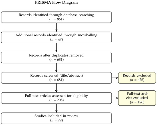
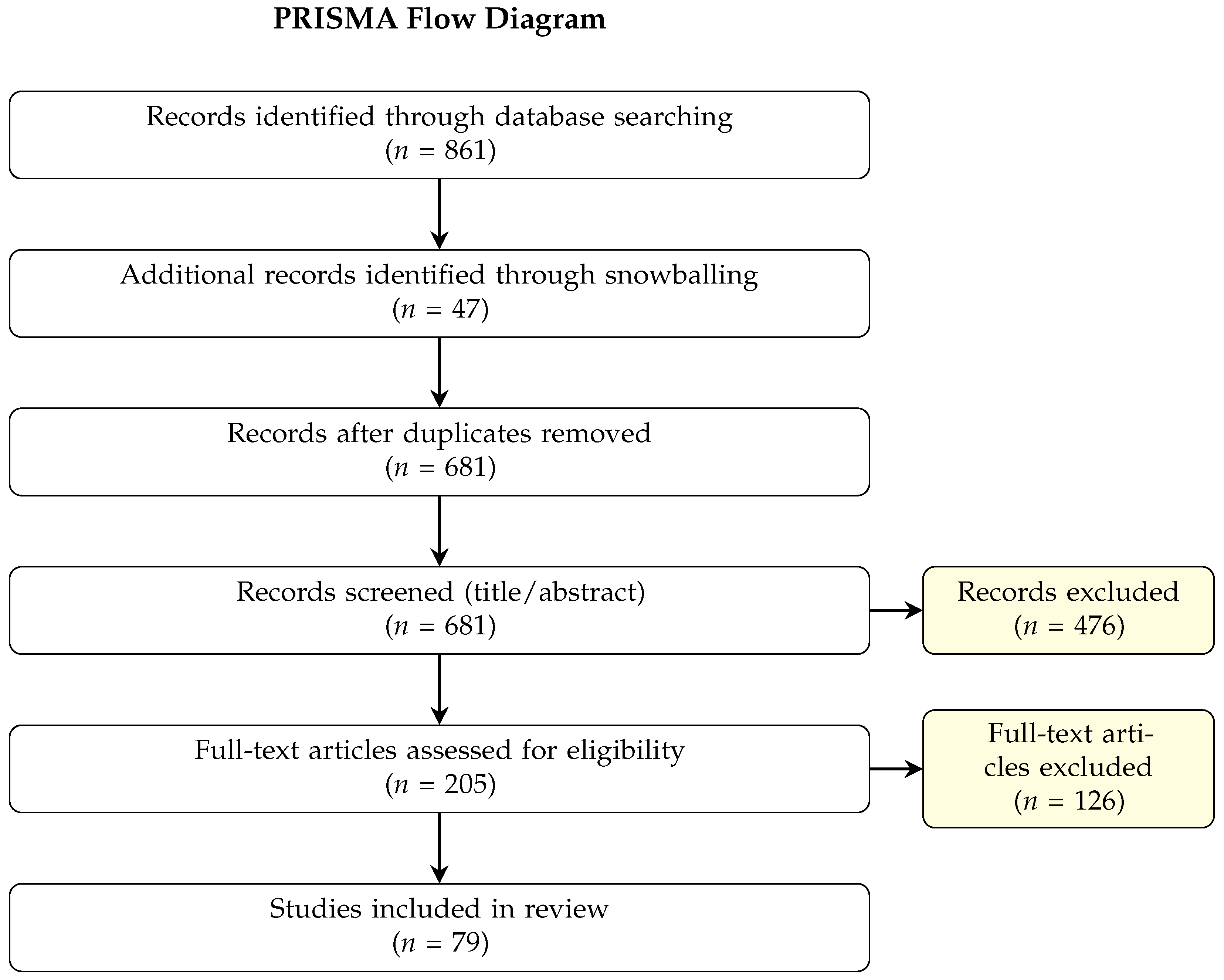
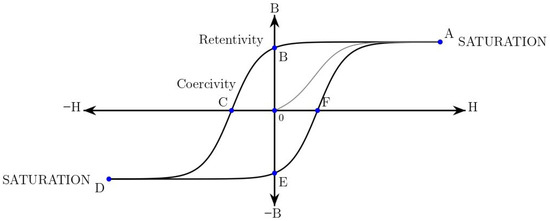
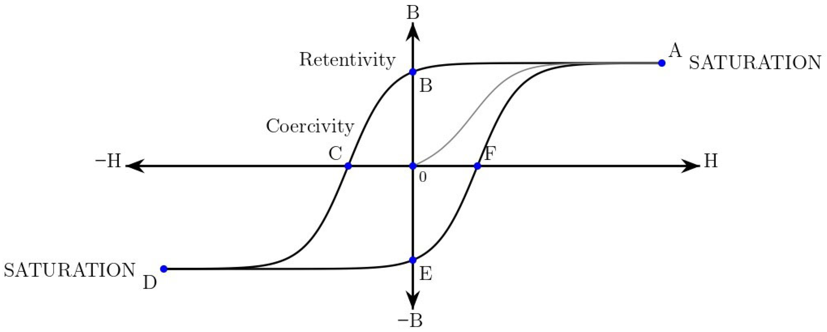
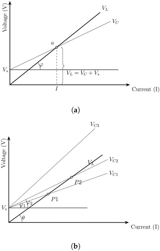
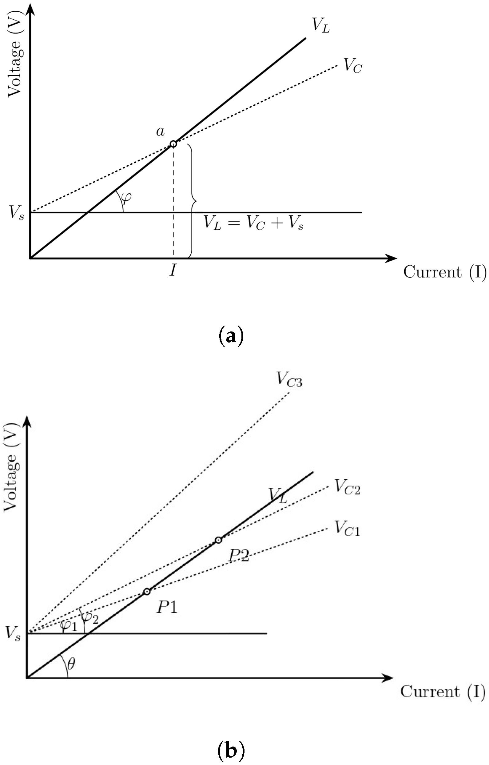
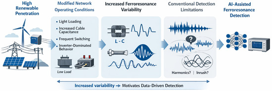
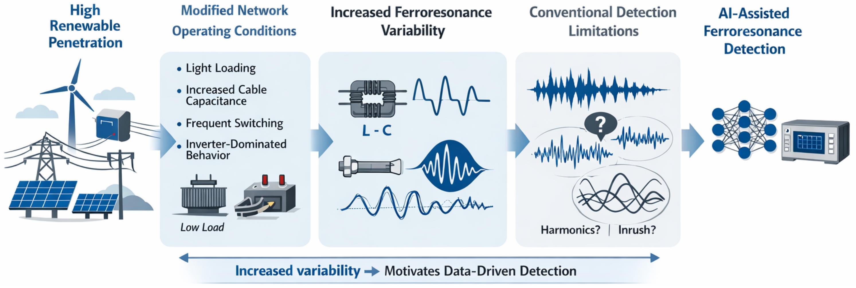

Disclaimer/Publisher’s Note: The statements, opinions and data contained in all publications are solely those of the individual author(s) and contributor(s) and not of MDPI and/or the editor(s). MDPI and/or the editor(s) disclaim responsibility for any injury to people or property resulting from any ideas, methods, instructions or products referred to in the content. |
© 2026 by the authors. Licensee MDPI, Basel, Switzerland. This article is an open access article distributed under the terms and conditions of the Creative Commons Attribution (CC BY) license.