Extra Dimensions in Quantum Newtonian Cosmology

Definition

This entry surveys the role of extra dimensions in Newtonian quantum cosmology, with particular emphasis on large, compactified, and warped dimensional geometries and their impact on the Newtonian potential in the early universe. The discussion begins with a review of Kaluza–Klein type toy models, followed by models with large extra dimensions in which gravity propagates into a higher-dimensional bulk, producing Yukawa-like modifications to the inverse-square law at submillimeter scales. Compactification schemes on toroidal and spherical dimensions are then examined, yielding the spectrum of Kaluza–Klein modes and quantifying their corrections to the Newtonian potential. Warped extra dimensions of the Randall–Sundrum type are also considered, in which a warp factor dimension is introduced; the resulting modifications to the Newtonian interaction in quantum-corrected cosmological settings are discussed in detail.

1. Introduction

Over the past century, nature has yielded tantalizing hints that our universe may be made up of more than the three familiar spatial dimensions that are directly accessible by traditional observation. In the early twentieth century, Kaluza and Klein [1,2,3,4,5,6,7] attempted to extend spacetime to five dimensions to unify gravitational and electromagnetic interactions.

Extra dimensions have since been invoked across a wide range of contexts, including

• addressing the hierarchy between the electroweak and Planck scales [8,9,10];
• providing the additional compact dimensions required by string theory [11,12,13,14];
• generating fermion and neutrino mass hierarchies [15] and additional sources of CP violation [16,17];
• supplying new mechanisms for inflation or other early-universe dynamics [18,19,20,21].

Although these additional dimensions are not directly perceived, their presence may be inferred through their influence on physical laws. Klein originally suggested that an extra dimension could be compactified on a circular geometry ($S^1$), with a radius on the order of the Planck length—small enough to remain hidden at observable energies. This idea has been expanded by modern theories, compactifying higher-dimensional spaces on more complex geometries such as tori, spheres, or Calabi–Yau shapes. The momentum along these compactified dimensions becomes quantized, much like a particle in a box. This results in a discrete spectrum of excitations known as Kaluza–Klein (KK) modes [2]. Although KK modes correspond to massive excitations, they are undetectable at current energies because their mass is inversely proportional to the compactification radius. With a radius near the Planck scale, the first KK excitation lies far beyond the reach of present-day accelerators. While these modes are currently beyond direct detection, they offer a distinctive prediction of extra-dimensional models.

Several theories have emerged with the goal of exploring the implications of higher-dimensional spacetimes [4,22,23,24]. Universal Extra Dimensions (UED) models allow Standard Model fields to propagate through all dimensions [25]. Other frameworks, like the Arkani-Hamed, Dimopoulos, Dvali (ADD) model, confine matter fields to a four-dimensional “brane” within a higher-dimensional bulk, allowing only gravity to access the full spacetime [8,26]. Randall–Sundrum (RS) models go further by introducing a warped geometry that localizes gravity near the brane [9,10].

The existence of extra dimensions has profound consequences for both classical and quantum theories of gravity. One of the most direct consequences is a modification to Newton’s inverse-square law at small distances, often expressed through Yukawa-type corrections [27,28,29]. These modifications to the gravitational potential are testable through precision experiments and may provide evidence for—or constraints on—extra-dimensional physics. This entry reviews several representative extra-dimensional frameworks and their gravitational signatures, focusing on how compactification and warping alter the Newtonian potential through Kaluza–Klein modes and short-distance departures from the inverse-square law, with applications to Newtonian quantum cosmology.

2. Toy Examples of Kaluza–Klein Extra Dimensions

This section introduces simple Kaluza–Klein toy models to motivate how extra dimensions influence physical observables in a controlled and transparent setting. Before analyzing the full gravitational consequences of higher-dimensional spacetimes, it is essential to understand how compact dimensions modify even the most elementary quantum mechanical systems. These models—such as a particle on a cylinder or a particle in a box with a compact extra coordinate—demonstrate explicitly how periodic boundary conditions quantize momentum along the compact dimension and give rise to a characteristic tower of massive KK modes. The resulting band structure, energy gaps, and suppression of extra-dimensional excitations at low energies provide intuitive insight into why extra dimensions may remain hidden at observable scales. Establishing these basic mechanisms lays the conceptual groundwork for later sections, where compactification geometries, KK spectra, and Newtonian potential corrections are developed in full generality. By starting with solvable toy examples, a foundation is established that clarifies how higher-dimensional physics manifests in both quantum and classical gravitational contexts.

The spacetime manifold is taken to be the direct product

$$M_4\times S^1,$$

where $M_4$ denotes the usual four-dimensional Minkowski space and $S^1$ is a circle of radius R. Equivalently, one may view this as a five-dimensional cylindrical geometry of radius R (see Figure 1 and Figure 2).

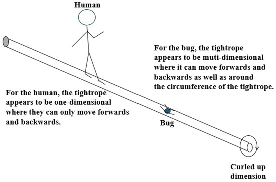
Figure 1. A heuristic analogy of a compactified circular Kaluza–Klein dimension along an infinite length dimension. At large scale, only the extended dimension can be observed, but at smaller scales the circular dimension can be probed.

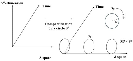
Figure 2. Compactification of an additional spatial dimension on $S^1$. The extra dimension is taken to be circular with radius R, so that the spacetime is effectively lower-dimensional at distances much larger than the compactification scale.

2.1. Free Particle on a Cylinder

One useful example that illustrates Kaluza–Klein compactification is a free particle that can move along an infinite cylinder with a finite radius R [30,31]. The wave function, $\psi (x,y)$, must obey periodic boundary conditions,

$$\psi (x,y)=\psi (x,y+2\pi R).$$

The dimension x is the infinite dimension in length, and the dimension y corresponds to $R\times \theta$. The free particle Hamiltonian for this system is given by

$$\widehat{H}=-{\displaystyle \frac{{\hslash }^2}{2m}}\left({\displaystyle \frac{{\partial }^2}{\partial x^2}}+{\displaystyle \frac{{\partial }^2}{\partial y^2}}\right),$$

(1)

where ℏ is the reduced Planck’s constant and m is the mass of the particle.

The wavefunctions $\psi (x,y)$ that satisfy this Hamiltonian are given by

$$\widehat{H}\psi (x,y)=E\psi (x,y),$$

(2)

along with the periodicity condition in y. The separation-of-variables technique is employed with a plane-wave ansatz,

$$\psi (x,y)=e^{i{k}_{x}x}{e}^{i{k}_{y}y},$$

(3)

where $k_x$ and $k_y$ are the wave numbers in the $x-$ and $y-$directions.

Substituting the ansatz into the Schrödinger equation,

$$\widehat{H}\psi (x,y)=-{\displaystyle \frac{{\hslash }^2}{2m}}\left(-k_x^2-k_y^2\right)\psi (x,y)$$

(4)

$$={\displaystyle \frac{{\hslash }^2}{2m}}(k_x^2+k_y^2)\psi (x,y),$$

(5)

yields the energy eigenvalues,

$$E(k_x,k_y)={\displaystyle \frac{{\hslash }^2}{2m}}\left(k_x^2+k_y^2\right).$$

(6)

The periodicity condition in y requires

$$\psi (x,y+2\pi R)=e^{i{k}_{x}x}{e}^{i{k}_y(y+2\pi R)}$$

(7)

$$\begin{array}{cc}\hfill & =e^{i{k}_{x}x}{e}^{i{k}_{y}y}{e}^{i2\pi R{k}_y}\hfill \end{array}$$

(8)

$$\begin{array}{cc}\hfill & =\psi (x,y)e^{i2\pi R{k}_y}.\hfill \end{array}$$

(9)

In order to preserve periodicity,

$$e^{i2\pi R{k}_y}=1\Rightarrow k_y={\displaystyle \frac{n}{R}},n\in \mathbb{Z}.$$

Thus, momentum in the compact direction is quantized. The energy levels allowed as a function of the quantum number n become

$$E_n\left(k_x\right)={\displaystyle \frac{{\hslash }^2}{2m}}\left(k_x^2+{\displaystyle \frac{n^2}{R^2}}\right),k_x\in \mathbb{R},n\in \mathbb{Z}.$$

(10)

Each value of the quantum number n defines a band of energy levels, continuous in the wave number $k_x$ but with a discrete offset. The minimum energy in each band is given by

$$E_n^{\min }={\displaystyle \frac{{\hslash }^2{n}^2}{2m{R}^2}}.$$

(11)

Although the Kaluza–Klein spectrum scales quadratically with n and the band spacings are therefore not evenly spaced, the compactification radius R defines a natural energy scale ${\hslash }^2/\left(2m{R}^2\right)$. This scale characterizes the lowest excitation above the ground band and determines the energy at which extra-dimensional effects first become relevant.

At low energies, only the quantum-number $n=0$ band is populated. This leads to

$$E\left(k_x\right)= {\displaystyle \frac{{\hslash }^2}{2m}}{k}_x^2,$$

(12)

$$\psi (x,y)= e^{i{k}_{x}x},$$

(13)

which is independent of the coordinate y. In this regime, the particle does not exhibit any dependence on the compact coordinate. The particle’s dynamics are effectively confined to the non-compact direction, corresponding to that of a one-dimensional free particle.

Furthermore, the $x-$ and $y-$momenta are

$${\widehat{p}}_x\psi =-i\hslash {\displaystyle \frac{\partial }{\partial x}}{e}^{i{k}_{x}x}=\hslash k_x\psi ,$$

(14)

$${\widehat{p}}_y\psi =-i\hslash {\displaystyle \frac{\partial }{\partial y}}{e}^{i{k}_{x}x}=0.$$

(15)

This confirms that there is no motion around the cylinder when the particle is in the ground state. The energy scale at which extra-dimensional effects become visible is

$$E_1={\displaystyle \frac{{\hslash }^2}{2m{R}^2}}.$$

(16)

Thus, for energies $E\ll E_1$, the compact dimension does not contribute to the dynamics, and the particle’s behavior is effectively that of a one-dimensional system.

2.2. Particle in a Box with a Kaluza–Klein Extra Dimension

Consider a particle of mass m in an infinite square well of width a in the x-direction, with an extra spatial dimension y compactified on a circle of radius R [11,31,32]. The time-independent Schrödinger equation in two dimensions is

$$-{\displaystyle \frac{{\hslash }^2}{2m}}\left({\displaystyle \frac{{\partial }^2}{\partial x^2}}+{\displaystyle \frac{{\partial }^2}{\partial y^2}}\right)\psi (x,y)=E\psi (x,y),$$

(17)

where the potential is given as

$$V(x,y)=\left\{\begin{array}{cc}0,\hfill & 0<x<a,\hfill \\ \infty ,\hfill & \mathrm{otherwise},\hfill \end{array}\right.y\sim y+2\pi R.$$

Assuming the separation of variables can be applied in this situation,

$$\psi (x,y)=X\left(x\right)Y\left(y\right).$$

This yields

$$-{\displaystyle \frac{{\hslash }^2}{2m}}\left(Y{X}^{″}+X{Y}^{″}\right)=EXY\Rightarrow -{\displaystyle \frac{{\hslash }^2}{2m}}{\displaystyle \frac{X^{″}}{X}}-{\displaystyle \frac{{\hslash }^2}{2m}}{\displaystyle \frac{Y^{″}}{Y}}=E,$$

where a prime indicates a spatial derivative. Defining

$$-{\displaystyle \frac{{\hslash }^2}{2m}}{\displaystyle \frac{X^{″}}{X}}=E_x,-{\displaystyle \frac{{\hslash }^2}{2m}}{\displaystyle \frac{Y^{″}}{Y}}=E_y,E_x+E_y=E,$$

the resulting equations separate.

Inside the infinite well, $0<x<a$, the x-equation along with its boundary conditions is given as

$$-{\displaystyle \frac{{\hslash }^2}{2m}}{X}^{″}\left(x\right)=E_{x}X\left(x\right),X\left(0\right)=X\left(a\right)=0.$$

Its normalized eigenfunctions and eigenvalues are familiar from the standard infinite particle-in-a-box solutions:

$$X_k\left(x\right)=\sqrt{{\displaystyle \frac{2}{a}}}sin\left({\displaystyle \frac{k\pi }{a}}x\right),k=1,2,\dots ,$$

(18)

$$E_x^{\left(k\right)}= {\displaystyle \frac{{\hslash }^2}{2m}}{\left({\displaystyle \frac{k\pi }{a}}\right)}^2.$$

(19)

On the circle $y\sim y+2\pi R$, the equation is

$$-{\displaystyle \frac{{\hslash }^2}{2m}}{Y}^{″}\left(y\right)= E_{y}Y\left(y\right),$$

or

$$Y^{″}+k_y^{2}Y=0,k_y^2={\displaystyle \frac{2m{E}_y}{{\hslash }^2}},$$

with periodic boundary condition $Y(y+2\pi R)=Y\left(y\right)$. Hence,

$$k_y={\displaystyle \frac{\mathcal{l}}{R}},\mathcal{l}\in \mathbb{Z},$$

and the wavefunction components may be taken as

$$Y_{\mathcal{l}}\left(y\right)=\left\{\begin{array}{cc}{\displaystyle \frac{1}{\sqrt{2\pi R}},}\hfill & \mathcal{l}=0,\hfill \\ {\displaystyle \frac{1}{\sqrt{\pi R}}cos\left(\frac{\mathcal{l}y}{R}\right)\mathrm{or}\frac{1}{\sqrt{\pi R}}sin\left(\frac{\mathcal{l}y}{R}\right),}\hfill & \mathcal{l}=1,2,\dots \hfill \end{array}\right.$$

(20)

The full wavefunctions and energies are

$${\psi }_{k,\mathcal{l}}(x,y)=X_k\left(x\right)Y_{\mathcal{l}}\left(y\right),$$

(21)

$$E_{k,\mathcal{l}}= E_x^{\left(k\right)}+E_y^{\left(\mathcal{l}\right)}= {\displaystyle \frac{{\hslash }^2}{2m}}\left[{\left({\displaystyle \frac{k\pi }{a}}\right)}^2+{\left({\displaystyle \frac{\mathcal{l}}{R}}\right)}^2\right].$$

(22)

For $\mathcal{l}=0$, this reduces to the usual 1D square-well spectrum.

The first excited extra-dimensional level has $\mathcal{l}=\pm 1$,

$$E_{1,1}= {\displaystyle \frac{{\hslash }^2}{2m}}\left[{\left({\displaystyle \frac{\pi }{a}}\right)}^2+{\left({\displaystyle \frac{1}{R}}\right)}^2\right]\approx {\displaystyle \frac{{\hslash }^2}{2m{R}^2}}(\mathrm{if}R\ll a),$$

provided that

$$E\ll {\displaystyle \frac{{\hslash }^2}{2m{R}^2}},$$

Thus, there are no $\mathcal{l}\ne 0$ excited modes and the system behaves effectively as an infinite one-dimensional square well.

3. Extra Dimension Models for Newtonian Potentials

The quantum-mechanical toy models introduced in the previous section demonstrate how compact extra dimensions lead to discrete Kaluza–Klein spectra and characteristic excitation scales. These same mechanisms reappear in the gravitational sector, where compactification modifies the form of the Newtonian potential through the exchange of massive KK modes.

Having established the basic quantum-mechanical consequences of compact extra dimensions through simple Kaluza–Klein toy models, the discussion turns to the implications for gravitational interactions at the Newtonian level. This section examines how the presence of additional spatial dimensions modifies the Poisson equation and, consequently, the form of the Newtonian potential [33,34,35,36] generated by a point mass. Both large and compactified extra-dimensional geometries are considered, with particular emphasis on how Kaluza–Klein excitations and image-mass constructions give rise to Yukawa-type corrections to the inverse-square law. These modified potentials provide a natural framework for incorporating extra-dimensional effects into Newtonian quantum cosmology and establish the groundwork for the warped geometries discussed in later sections.

For reference, Table 1 provides a compact summary of the extra-dimensional frameworks reviewed in this section, emphasizing how the underlying geometry and Kaluza–Klein spectrum translate into characteristic deviations from the inverse-square law. This table is intended as a guide to the detailed discussions presented in the following subsections.

Table 1. Schematic comparison of extra-dimensional scenarios and their leading modifications to the Newtonian potential.

Scenario	Geometry/Setup	KK Spectrum	Newtonian Potential
Large (uncompactified) dimensions	${\mathbb{R}}^d$ with $d=D-1$ spatial dimensions	continuous	${\mathrm{\Phi }}_D\left(r\right)\propto r^{-(d-2)}$ ($d>2$),   ${\mathrm{\Phi }}_3\left(r\right)\propto lnr$ $(d=2)$
Single compact dimension (circle)	${\mathbb{R}}^3\times S^1$ with period R	discrete tower/images	${\displaystyle V\left(r\right)\simeq -\frac{G_{4}M}{r}}$${\displaystyle \times \left[1+\mathcal{O}\left(e^{-2\pi r/R}\right)\right]}$
Toroidal compactification	${\mathbb{R}}^3\times T^n$ (radii $R_i$)	discrete KK	${\displaystyle V\left(r\right)\simeq -\frac{G_{4}M}{r}}$${\displaystyle \times \left[1+\sum _{\overrightarrow{m}\ne 0}{C}_{\overrightarrow{m}}{e}^{-m_{\overrightarrow{m}}r}\right]}$
Spherical compactification	${\mathbb{R}}^3\times S^n\left(R\right)$	discrete Laplacian spectrum	${\displaystyle V\left(r\right)\simeq -\frac{G_{4}M}{r}}$${\displaystyle \times \left[1+C_1{e}^{-{\mu }_{1}r}+\dots \right]}$
Calabi–Yau compactification	$M_4\times {\mathcal{X}}_6$ with vanishing Ricci curvature on a Kähler manifold	model-dependent discrete spectrum	${\displaystyle V\left(r\right)\simeq -\frac{G_{4}M}{r}}$${\displaystyle \times \left[1+\sum _{j\ge 1}{c}_j{e}^{-m_{j}r}\right]}$
Warped extra dimensions (RS1/RS2)	AdS5 bulk with warp scale k; brane-localized observers	RS1: discrete; RS2: continuum (suppressed coupling)	${\displaystyle V\left(r\right)\simeq -\frac{G_{4}M}{r}}$${\displaystyle \times \left[1+\frac{\alpha }{{\left(kr\right)}^2}+\dots \right]}$

3.1. Large Dimensions

In this section, Newtonian gravity is reviewed in a D–dimensional spacetime with $d=D-1$ spatial dimensions. Treating the gravitational field as a flux field in ${\mathbb{R}}^d$, Gauss’ law fixes the radial falloff of the field sourced by a point mass: the flux through the boundary of a d-ball is constant, so the field scales as $g_D\left(r\right)\propto r^{-(d-1)}$. The radial integration then yields the corresponding gravitational potential ${\mathrm{\Phi }}_D\left(r\right)\propto r^{-(d-2)}$ for $d>2$, with logarithmic behavior recovered in the special case $d=2$. These results provide a baseline against which compactification and localization mechanisms can be compared, since any extra dimensions that remain large and flat at macroscopic scales would produce deviations from the observed inverse-square law.

For a point mass M at the origin, the mass density is

$$\rho \left(\mathbf{x}\right)=M{\delta }^{\left(d\right)}\left(\mathbf{x}\right),d=D-1,$$

where D is the number of spacetime dimensions and d is the number of spatial dimensions.

The D-dimensional Poisson equation is

$${\nabla }_{\left(d\right)}^2{\mathrm{\Phi }}_D\left(\mathbf{x}\right)={\mathrm{\Omega }}_d{G}_D\rho \left(\mathbf{x}\right),$$

where $G_D$ is the fundamental gravitational constant in D spacetime dimensions and ${\mathrm{\Omega }}_d$ is the total solid angle in d spatial dimensions (equivalently, the surface area of the unit $(d-1)$-sphere).

Integrating over a d-ball $B_d\left(R\right)$ of radius R and applying the divergence theorem gives Gauss’ law

$${\oint }_{S^{d-1}\left(R\right)}{\mathbf{g}}_D·d\mathbf{A}=-{\mathrm{\Omega }}_d{G}_{D}M,$$

with ${\mathbf{g}}_D=-\nabla {\mathrm{\Phi }}_D$ the gravitational field and

$$d\mathbf{A}=\widehat{\mathbf{r}}dA,dA=R^{d-1}d{\mathrm{\Omega }}_d.$$

The volume of the unit d-ball and the solid angle of the unit $(d-1)$-sphere (see Solid Angle, Surface Area, and Volume) are

$$V_d\left(1\right)={\displaystyle \frac{{\pi }^{d/2}}{\Gamma \left(\frac{d}{2}+1\right)}},{\mathrm{\Omega }}_d={\displaystyle \frac{2{\pi }^{d/2}}{\Gamma \left(\frac{d}{2}\right)}}.$$

Hence, the surface area of the radius-R sphere $S^{d-1}\left(R\right)$ is

$$A_d\left(R\right)={\oint }_{S^{d-1}\left(R\right)}dA={\mathrm{\Omega }}_d{R}^{d-1},\mathrm{so}\mathrm{that}{A}_d\left(1\right)={\mathrm{\Omega }}_d.$$

Spherical symmetry implies ${\mathbf{g}}_D\left(r\right)=g_D\left(r\right)\widehat{\mathbf{r}}$, so Gauss’ law reads

$$g_D\left(r\right)A_d\left(r\right)=-{\mathrm{\Omega }}_d{G}_{D}M.$$

Therefore,

$$g_D\left(r\right)=-{\displaystyle \frac{G_{D}M}{r^{d-1}}}=-{\displaystyle \frac{G_{D}M}{r^{D-2}}}.$$

Because $g_D\left(r\right)=-d{\mathrm{\Phi }}_D/dr$, integration yields

$${\mathrm{\Phi }}_D\left(r\right)=-{\displaystyle \frac{G_{D}M}{(d-2)r^{d-2}}}+C,d>2,$$

where the additive constant, C, is chosen so that ${\mathrm{\Phi }}_D\left(r\right)\to 0$ as $r\to \infty$. For $d=2$, the potential becomes logarithmic, ${\mathrm{\Phi }}_2\left(r\right)\propto -G_{D}Mln(r/r_0)$.

The corresponding magnitude of the force between two point masses is

$$F_D\left(r\right)={\displaystyle \frac{G_D{m}_1{m}_2}{r^{d-1}}}={\displaystyle \frac{G_D{m}_1{m}_2}{r^{D-2}}}.$$

For $D=4$ and $d=3$, one identifies $G_4$ with the usual four–dimensional spacetime Newton gravitational constant and obtains the usual inverse-square law. Experiments [28,37,38,39] confirm this behavior down to submillimeter scales, so truly infinite extra dimensions are excluded by observation, which motivates the compactification mechanisms considered in the next section.

3.2. Compactified Dimensions

Although the specific geometry of the compact internal space differs between toroidal, spherical, and Calabi–Yau compactifications, the resulting corrections to Newtonian gravity share a common physical origin. In each case, deviations from the inverse-square law arise from the spectrum and degeneracies of Kaluza–Klein modes associated with the compact dimensions.

In many phenomenologically viable models, the extra spatial dimensions are compactified with characteristic radii small enough to evade current experimental bounds. In the context of ADD-type scenarios, the number of extra dimensions n is typically taken between 2 and 7: with only a single extra dimension, deviations from Newtonian gravity would extend over astronomical distances, while $n=7$ corresponds to the highest-dimensional consistent supergravity theory in eleven dimensions [8,27,29,40].

A common parameterization of short-distance deviations from Newtonian gravity is

$$V\left(r\right)=-{\displaystyle \frac{G_{4}M}{r}}\left(1+\alpha e^{-r/\lambda }\right),$$

where $\alpha$ sets the strength and $\lambda$ the range of the Yukawa correction.

3.2.1. Compactification on a Torus

When considering toroidal compactification [41,42,43,44,45], the parameter

$$\alpha =2n,$$

where n is the number of extra spatial dimensions. With n being between 2 and 7, this allows $\alpha$ to take values of 4, 6, 8, ..., and 14 [46].

Toroidal compactification entails compactifying each extra dimension on a circle, producing a flat, periodic geometry (see Figure 3). This is an analytically convenient choice, as these periodic conditions give rise to a discrete and symmetric KK spectrum [41].

Figure 3. The above graphic gives a schematic illustration of the periodic boundary conditions associated with a torus.

In a toroidal geometry, the parameters governing the compactified dimensions can be separated into size moduli and shape moduli. The size modulus is determined by the physical lengths of the compactification radii $R_i$, while the shape modulus describes the relative orientation of the compact dimensions. In the case of two compact dimensions, the shape modulus specifies the angle $\theta$ between their fundamental cycles. Together, these moduli influence both the gravitational potential and the spectrum of KK modes [12,47].

For two orthogonal extra dimensions, the KK masses are given by

$$m_{\mathrm{KK}}^2={\displaystyle \frac{p^2}{R_1^2}}+{\displaystyle \frac{q^2}{R_2^2}},$$

where p and q are the lattice indices counting the number of loops along $R_1$ and $R_2$, respectively.

The corresponding gravitational potential for two orthogonal extra dimensions with radii $R_1$ and $R_2$ is

$$V\left(r\right)=-G_{6}M\sum _{q=-\infty }^{\infty }\sum _{p=-\infty }^{\infty }{\displaystyle \frac{1}{{\left(r^2+p^2{R}_1^2+q^2{R}_2^2\right)}^{3/2}}},$$

where $G_6$ is the six-dimensional Newton’s constant, analogous to $G_4$ but in a spacetime with two extra spatial dimensions. This double sum accounts for the contributions of all images of the source mass across the compact space. The index pair $(p,q)$ denotes the mirrored mass being considered: $(0,0)$ represents the “real” mass, $(1,0)$ is the image one loop around the first dimension, and $(0,1)$ is the image one loop around the second. Negative integers correspond to loops in the opposite direction. The $r^{-3}$ dependence reflects the falloff in the Newtonian potential as the winding numbers increase, ensuring the series converges.

These indices form the periodic lattice of image masses that characterize the compact space. The magnitude and pattern of deviations from Newtonian gravity in such a configuration are determined by $R_1$, $R_2$, and $\theta$, and can be probed in short-range gravitation experiments [48,49]. This formalism will be useful when comparing toroidal compactification to other geometries, including spherical compactification, which is covered in the following section.

3.2.2. Compactification on a Sphere Using Poisson’s Equation

Consider a scenario in which n extra spatial dimensions are compactified on an n-dimensional sphere $S^n$ of radius R (see Figure 4).

Figure 4. The above graphic gives a schematic illustration of the periodic boundary conditions associated with a sphere.

In the Newtonian limit of Einstein gravity in $D=(4+n)$ spacetime dimensions, the gravitational potential $V_{4+n}(\overrightarrow{r},\overrightarrow{x})$ generated by a point mass M satisfies the Poisson equation in $d=(3+n)$ spatial dimensions:

$${\nabla }_{(3+n)}^2{V}_{4+n}(\overrightarrow{r},\overrightarrow{x})={\mathrm{\Omega }}_{n+3}{G}_{4+n}M{\delta }^{(3+n)}(\overrightarrow{r},\overrightarrow{x}),$$

(23)

where $\overrightarrow{r}\in {\mathbb{R}}^3$ denotes the coordinates in the extended spatial dimensions, $\overrightarrow{x}\in S^n$ are the coordinates on the compact internal space, $G_{4+n}$ is the Newton constant in $(D=4+n)$ dimensions, and ${\mathrm{\Omega }}_{n+3}$ denotes the surface area of a unit $(n+2)$-sphere (see Solid Angle, Surface Area, and Volume)

$${\mathrm{\Omega }}_{n+3}={\displaystyle \frac{2{\pi }^{(n+3)/2}}{\mathrm{\Gamma }\left(\frac{n+3}{2}\right)}}.$$

(24)

The potential can be expanded in a complete set of orthonormal eigenfunctions of the Laplace operator on $S^n$:

$$V_{4+n}(\overrightarrow{r},\overrightarrow{x})=\sum _{m=0}^{\infty }{V}_m\left(r\right){\mathrm{\Psi }}_m\left(\overrightarrow{x}\right),$$

(25)

where the eigenfunctions, so-called scalar hyper-spherical harmonics—which are a generalization of the standard spherical harmonics $Y_{\mathcal{l}m}(\theta ,\varphi )$ (note that is m the quantum number, not the KK index)—${\mathrm{\Psi }}_m$ satisfy the eigenvalue equation,

$${\nabla }_{S^n}^2{\mathrm{\Psi }}_m\left(\overrightarrow{x}\right)=-{\mu }_m^2{\mathrm{\Psi }}_m\left(\overrightarrow{x}\right),$$

(26)

with corresponding eigenvalues ${\mu }_m^2$. Inserting this ansatz into the Poisson equation leads to the radial equation for each mode,

$${\nabla }_3^2{V}_m\left(r\right)-{\mu }_m^2{V}_m\left(r\right)={\mathrm{\Omega }}_{n+3}{G}_{4+n}M{\mathrm{\Psi }}_m^{*}\left(0\right){\delta }^{\left(3\right)}\left(\overrightarrow{r}\right).$$

(27)

The solution to this Yukawa-type equation in three spatial dimensions is given by

$$V_m\left(r\right)=-{\displaystyle \frac{{\mathrm{\Omega }}_{n+3}{G}_{4+n}M{\mathrm{\Psi }}_m^{*}\left({\overrightarrow{x}}_0\right)}{4\pi }}{\displaystyle \frac{e^{-{\mu }_{m}r}}{r}}.$$

(28)

Consequently, the full potential takes the form

$$V_{4+n}(\overrightarrow{r},\overrightarrow{x})=-{\displaystyle \frac{{\mathrm{\Omega }}_{n+3}{G}_{4+n}M}{4\pi r}}\sum _{m=0}^{\infty }{\mathrm{\Psi }}_m^{*}\left(0\right){\mathrm{\Psi }}_m\left(\overrightarrow{x}\right)e^{-{\mu }_{m}r}.$$

(29)

Evaluating the potential at the source location in the compact space, $\overrightarrow{x}=0$, the sum over hyper-spherical harmonics in Equation (29) reduces to a sum over all degenerate eigenfunctions sharing the same eigenvalue ${\mu }_m^2$,

$$V_4\left(r\right)=-{\displaystyle \frac{G_{4}M}{r}}\sum _{m=0}^{\infty }\left(\sum _{\mathrm{degenerate}{\mathrm{\Psi }}_m}{\mathrm{\Psi }}_m^{*}\left(0\right){\mathrm{\Psi }}_m\left(0\right)\right)e^{-{\mu }_{m}r}.$$

(30)

By orthonormality and completeness of the scalar hyper-spherical harmonics, the inner sum evaluates to the degeneracy factor $d_m$, resulting in the four-dimensional effective potential,

$$V_4\left(r\right)=-{\displaystyle \frac{G_{4}M}{r}}\sum _{m=0}^{\infty }{d}_m{e}^{-{\mu }_{m}r},$$

(31)

where $G_4$ denotes the four-dimensional Newton constant, obtained by integrating out the compact internal space. For compactification on an n-sphere $S^n$ of radius R, the higher-dimensional gravitational constant $G_{(4+n)}$ is related to $G_4$ by

$$G_4={\displaystyle \frac{G_{(4+n)}}{\mathrm{Vol}\left(S^n\right)}}={\displaystyle \frac{G_{(4+n)}}{\frac{{\mathrm{\Omega }}_{n+1}}{n+1}{R}^{n+1}}},$$

(32)

where ${\mathrm{\Omega }}_{n+1}=2{\pi }^{(n+1)/2}/\mathrm{\Gamma }\left((n+1)/2\right)$ is the total solid angle of the unit n-sphere.

The eigenvalues and degeneracies of the Laplacian on the n-sphere are known analytically,

$${\mu }_m={\displaystyle \frac{\sqrt{m(m+n-1)}}{R}},m=0,1,2,\dots ,$$

(33)

$$d_m={\displaystyle \frac{(2m+n-1)(m+n-2)!}{(n-1)!m!}}.$$

(34)

Thus, the four-dimensional gravitational potential becomes

$$V_4\left(r\right)=-{\displaystyle \frac{G_{4}M}{r}}\sum _{m=0}^{\infty }{d}_{m}exp\left(-{\displaystyle \frac{\sqrt{m(m+n-1)}}{R}}r\right).$$

(35)

At large distances ($r\gg R$), the contribution of the lowest nontrivial Kaluza–Klein mode ($m=1$) dominates, leading to a Yukawa-type correction to Newton’s inverse-square law,

$$V_4\left(r\right)\approx -{\displaystyle \frac{G_{4}M}{r}}\left[1+(n+1)e^{-\sqrt{n}r/R}+\cdots \right].$$

(36)

This result demonstrates that compactification on $S^n$ modifies the gravitational potential in four dimensions through an infinite tower of exponentially suppressed Yukawa corrections. The strength of the leading-order correction is determined by the degeneracy of the first excited Kaluza–Klein level, given by $n+1$, while the range is controlled by the inverse of its mass, $R/\sqrt{n}$.

3.2.3. Compactification on a Circle Using Gauss’ Law

In order to see how a single compact extra dimension modifies Newtonian gravity, one may first analyze a toy model with four spatial dimensions $(x,y,z,w)$ in which the w-direction is compactified on a circle of circumference R:

$$w\equiv w+R.$$

(37)

The Gauss’ law for the gravitational field ${\mathbf{g}}_D$ of a point mass M in d spatial dimensions reads as follows.

$${\oint }_{S^{d-1}\left(r\right)}{\mathbf{g}}_D·d\mathbf{A}=-{\mathrm{\Omega }}_d{G}_{D}M,$$

(38)

where $G_D$ is Newton’s constant in $D=d+1$ spacetime dimensions and

$${\mathrm{\Omega }}_d={\displaystyle \frac{2{\pi }^{d/2}}{\mathrm{\Gamma }(d/2)}}$$

(39)

is the total solid angle in d-dimensions (equivalently, the surface area of the unit $(d-1)$-sphere). Because the gravitational field, ${\mathbf{g}}_D$, is spherically symmetric, its magnitude depends only on the radial coordinate r; Equation (38) implies the magnitude

$$g_D\left(r\right)={\displaystyle \frac{G_{D}M}{r^{d-1}}}.$$

(40)

With one extra dimension, the relevant spatial dimensionalities are

$$d=4(r\ll R),d=3(r\gg R).$$

Hence

$$r\ll R:g_4\left(r\right)={\displaystyle \frac{G_{5}M}{r^3}},V\left(r\right)=-{\displaystyle \frac{G_{5}M}{2r^2}},$$

(41)

$$r\gg R:g_3\left(r\right)={\displaystyle \frac{G_{4}M}{r^2}},V\left(r\right)=-{\displaystyle \frac{G_{4}M}{r}}.$$

(42)

For $r\gg R$, the string of “image” masses looks like a homogeneous line of density

$$\lambda ={\displaystyle \frac{M}{R}}.$$

Choose a four-dimensional Gaussian cylinder of length L and three-sphere end-caps of radius r. The total four-dimensional flux is $4\pi r^{2}L{g}_5\left(r\right)$, while the enclosed mass equals $\left({\displaystyle \frac{ML}{R}}\right)$. Substituting into Equation (38) with $d=4$ gives

$$4\pi r^{2}L{g}_5={\mathrm{\Omega }}_4{G}_5{\displaystyle \frac{ML}{R}}\Rightarrow g_5\left(r\right)={\displaystyle \frac{{\mathrm{\Omega }}_4}{4\pi }}{\displaystyle \frac{G_{5}M}{R{r}^2}}.$$

Comparing with the familiar $g_4=G_{4}M/r^2$, one finds

$$G_4={\displaystyle \frac{{\mathrm{\Omega }}_4}{4\pi }}{\displaystyle \frac{G_5}{R}}\Rightarrow G_5={\displaystyle \frac{4\pi }{{\mathrm{\Omega }}_4}}R{G}_4={\displaystyle \frac{2}{\pi }}R{G}_4,$$

(43)

because ${\mathrm{\Omega }}_4=2{\pi }^2$.

A point mass M at $(r,w)=(0,0)$ is accompanied by an infinite tower of image masses at $w=lR$ ($l\in \mathbb{Z}$). The four-dimensional potential therefore reads

$$V\left(r\right)=-{\displaystyle \frac{G_{5}M}{2}}\sum _{l=-\infty }^{\infty }{\displaystyle \frac{1}{r^2+l^2{R}^2}},$$

(44)

with $G_5$ already expressed via Equation (43). Introduce the dimensionless ratio $\mathrm{\Delta }\equiv r/R$, factor out $R^2$ from the denominator, and convert the summation to the standard form

$$V\left(r\right)=-{\displaystyle \frac{G_{4}M}{\pi R}}\sum _{l=-\infty }^{\infty }{\displaystyle \frac{1}{l^2+{\mathrm{\Delta }}^2}}.$$

(45)

These results reproduce the expected limiting behaviors: for $r\ll R$, the potential reduces to the four-spatial-dimensional form $V\left(r\right)\simeq -G_{5}M/\left(2r^2\right)$, while for $r\gg R$, the image sum approaches the three-dimensional Newtonian potential $V\left(r\right)\simeq -G_{4}M/r$ with corrections that are exponentially suppressed in $r/R$. Accordingly, compactification on a circle provides a simple benchmark illustrating how a finite compactification scale interpolates between higher- and lower-dimensional gravitational laws.

3.3. Compactification on Calabi–Yau Manifolds

A Calabi–Yau manifold is a compact, Kähler complex manifold with vanishing first Chern class [50,51,52,53]. A manifold is a geometric space that, near each point, looks like ordinary Euclidean space. For example, an ant walking on Earth’s surface experiences its surroundings as flat, even though the planet is a curved sphere. A Calabi–Yau manifold is a complex geometric space (see Figure 5) that ensures it admits a Ricci-flat metric—meaning its Ricci curvature tensor is zero. Calabi–Yau manifolds are central to string theory—they compactify the extra dimensions into shapes that determine fundamental particle interactions [54,55,56,57].

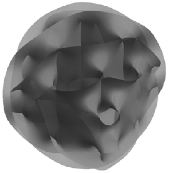
Figure 5. A visual representation of a Calabi–Yau manifold, shown as a three-dimensional projection to illustrate its intricate, folded geometry.

The geometry of moduli spaces of Calabi–Yau manifolds, including their deformations and mirror symmetry, is developed in Refs. [58,59,60,61,62,63,64]. As a simple example of a compact manifold (not necessarily Calabi–Yau), a d-sphere may be embedded in ${\mathbb{R}}^{d+1}$ as

$$x_1^2+\cdots +x_{d+1}^2=R^2,$$

(46)

where R is the radius of the sphere.

In specific Calabi–Yau constructions that possess enhanced discrete symmetries, most notably symmetric product orbifolds, the structure of low-lying states can be organized by discrete global symmetry groups generated by products of permutation groups ${\mathfrak{S}}_d$ and cyclic factors ${\mathbb{Z}}_{\mathcal{l}}^d$ [65].

Irreducible representations (irreps) of ${\mathfrak{S}}_d$ are specified by integer partitions $\left\{m_i\right\}$ of d obeying

$$m_1\ge m_2\ge \cdots \ge m_d\ge 0,m_1+m_2+\cdots +m_d=d,$$

(47)

with dimension given by

$$d_m={\displaystyle \frac{d!}{h_1!h_2!\cdots h_n!}}\prod _{i<j}(h_i-h_j),h_i\equiv m_i+d-i.1$$

(48)

3.3.1. Massless State

The trivial representation with $m_1=d$, $m_{2,3,\dots ,d}=0$ corresponds to the universal CY property $h^{0,0}=1$. This state is a singlet under both ${\mathfrak{S}}_d$ and ${\mathbb{Z}}_{\mathcal{l}}^d$.

3.3.2. First Massive State

The lowest nontrivial irrep occurs for

$$m_1=m_2=\cdots =m_d=1.$$

This representation is one-dimensional under ${\mathfrak{S}}_d$, but degeneracy arises from the action of ${\mathbb{Z}}_{\mathcal{l}}^d$, so its multiplicity is at least $d^{\mathcal{l}}$.

3.3.3. Bounds on Degeneracy

In the absence of any symmetries, the degeneracy of the first massive state is of order unity [66]:

$$d_{\mathrm{lower}}=\mathcal{O}\left(1\right).$$

(49)

For a “maximally symmetric” case, namely the isotropic quintic, the global symmetry is isomorphic to the semi-direct product ${\mathfrak{S}}_5⋉{\mathbb{Z}}_5^4$. In this case, the degeneracy of the first massive state attains the upper bound

$$d_{\mathrm{upper}}=20.$$

(50)

In summary, Calabi–Yau compactifications provide a broad and geometrically rich class of internal spaces in which both topology and symmetry can strongly influence the organization and degeneracies of low-lying states. Although the discussion above highlights idealized symmetry limits, most Calabi–Yau manifolds possess only limited discrete symmetry, so the generic expectation is that degeneracies are modest, with occasional enhancements in highly symmetric examples. These observations motivate treating Calabi–Yau compactification as a complementary benchmark to the toroidal and spherical cases discussed previously, and they provide context for the more model-dependent scenarios considered next.

4. Warped Extra Dimensions

The compactification scenarios considered thus far assume factorizable geometries characterized by a fixed compactification scale. Warped extra-dimensional models represent a qualitatively distinct realization, in which the background geometry itself localizes gravity and alters the contribution of massive modes to the effective four-dimensional potential.

In warped extra-dimensional models, the higher-dimensional spacetime is not a simple direct product but instead possesses a non-factorizable metric of the form

$$d{s}^2=e^{-2k\left|y\right|}{g}_{\mu \nu }\left(x\right)d{x}^{\mu }d{x}^{\nu }+d{y}^2,$$

where $g_{\mu \nu }\left(x\right)$ is the induced four-dimensional metric on the brane and y parametrizes the extra spatial dimension. The manifold $M_4$ denotes the effective four-dimensional spacetime experienced by observers confined to the brane, while the parameter k sets the curvature scale of the five-dimensional Anti–de Sitter (AdS₅) bulk and controls the strength of the warping along the extra dimension. Physically, $k^{-1}$ defines the characteristic length scale over which gravitational interactions transition from higher-dimensional behavior to the effective four-dimensional Newtonian regime. In the context of Newtonian quantum cosmology, this warping scale determines both the localization of the graviton zero mode responsible for recovering Newton’s inverse-square law and the magnitude of quantum and semiclassical corrections arising from the continuum of massive Kaluza–Klein modes.

Randall and Sundrum Warped Dimensions

In 1999, Randall and Sundrum [9,10,67,68,69,70] proposed a five-dimensional warped-geometry scenario to resolve the hierarchy problem. This framework also admits a natural solution to the flavor problem and permits gauge–coupling unification of the Standard Model. Two variants of the model exist: RS I [71,72,73,74], in which two four-dimensional boundary branes are embedded in an AdS₅ bulk (see Figure 6), and RS II [75,76,77], which contains a single brane. In both cases, Standard Model fields are confined to the brane(s), while gravity propagates throughout the five-dimensional bulk, modifying the Newtonian potential at large separations:

$$V\left(r\right)\simeq -{\displaystyle \frac{G_4{m}_1{m}_2}{r}}\left(1+{\displaystyle \frac{2}{3k^2{r}^2}}\right),r\gg {\displaystyle \frac{1}{k}},$$

where k is a parameter that characterizes the curvature of the extra dimension and $k^{-1}$ sets the curvature (or “warping”) scale of the extra dimension.

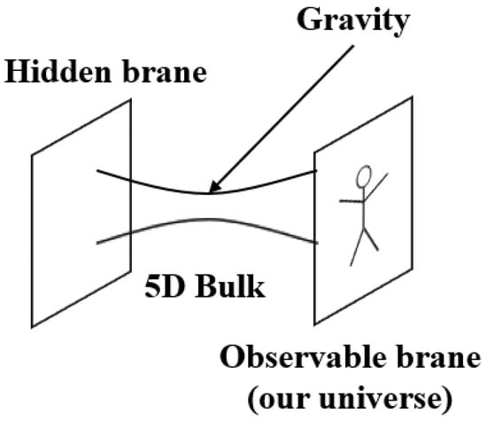
Figure 6. A schematic illustration of the Randall–Sundrum warped extra dimension, showing the localization of gravity near the brane.

The extra dimension itself is compactified on an $S^1/{\mathbb{Z}}_2$ orbifold: one begins with a circle of circumference $2\pi R$, parameterized by $y\sim y+2\pi R$, and then identifies $y\sim -y$. This “folds” the circle into the interval $0\le y\le \pi R$, with the endpoints $y=0$ and $y=\pi R$ fixed under the reflection $y\mapsto -y$. These fixed points correspond to the Planck brane, at which the four-dimensional Planck scale is defined and where gravity is most strongly localized, and the TeV brane, where the local energy scales are red-shifted by the warp factor

$$e^{-\pi kR},$$

thereby generating a large hierarchy between the Planck and electroweak scales.

This section presents a heuristic treatment of the Newtonian potential’s modification. In the single-brane Randall–Sundrum model (RS II), the background metric is given by

$$d{s}^2=e^{-2k\left|y\right|}{\eta }_{\mu \nu }d{x}^{\mu }d{x}^{\nu }+d{y}^2,$$

(51)

where $k^{-1}$ is the curvature length of the bulk and the visible brane is located at $y=0$, ${\eta }_{\mu \nu }$ is the Minkowski metric, $d{x}^{\mu }$ are the infinitesimal coordinate differentials, and $dy$ is the coordinate differential of the extra dimension.

The linearized graviton fluctuation in 5D is decomposed as

$$h_{\mu \nu }(x,y)=\sum _{n=0}^{\infty }{h}_{\mu \nu }^{\left(n\right)}\left(x\right){\psi }_n\left(y\right),$$

(52)

where $h_{\mu \nu }^{\left(n\right)}\left(x\right)$ are the four-dimensional graviton modes, and the extra–dimensional profiles of ${\psi }_n\left(y\right)$ satisfy a one-dimensional Schrödinger equation. A normalizable zero mode (where N is the normalization factor) ${\psi }_0\left(y\right)=N{e}^{-2k\left|y\right|}$ reproduces four-dimensional gravity, while the continuum of massive KK modes, labeled by a continuous mass parameter $m>0$, is suppressed on the brane,

$$|{\psi }_m{\left(0\right)|}^2\simeq {\displaystyle \frac{m}{2k}}.$$

(53)

For two point masses $m_1$ and $m_2$ fixed at $y=0$ the potential is obtained from the 00-component of the propagator evaluated on the brane,

$$V\left(r\right)=-{\displaystyle \frac{m_1{m}_2}{M_5^3}}\left[|{\psi }_0{\left(0\right)|}^2{\mathcal{G}}_0\left(r\right)+{\int }_0^{\infty }dm\rho \left(m\right){\left|{\psi }_m\left(0\right)\right|}^2{\mathcal{G}}_m\left(r\right)\right],$$

(54)

where $\rho \left(m\right)dm$ is the continuum density of KK states,

$${\mathcal{G}}_0\left(r\right)={\displaystyle \frac{1}{4\pi r}}$$

(55)

is the massless Green function, and

$${\mathcal{G}}_m\left(r\right)={\displaystyle \frac{e^{-mr}}{4\pi r}}$$

(56)

is the effective massive (Yukawa) Green’s function.

The first term reproduces Newton’s law. Matching $m_1{m}_2/M_5^3{\left|{\psi }_0\left(0\right)\right|}^2=G_4{m}_1{m}_2$ fixes the four-dimensional Newton constant,

$$G_4={\displaystyle \frac{k}{M_5^3}}\left(1-e^{-2k\pi R}\right),$$

(57)

which reduces to $G_4=k/M_5^3$ in the non-compact limit $R\to \infty$.

Making the heuristic replacements

$$\rho \left(m\right)dm\simeq dm,|{\psi }_m{\left(0\right)|}^2\simeq {\displaystyle \frac{m}{2k}},$$

(58)

and inserting ${\mathcal{G}}_m\left(r\right)$, the KK integral in (54) becomes

$$\begin{array}{cc}\hfill \delta V\left(r\right)& \equiv -{\displaystyle \frac{m_1{m}_2}{M_5^3}}{\displaystyle \frac{1}{2k}}{\int }_0^{\infty }dmm{\displaystyle \frac{e^{-mr}}{4\pi r}}\hfill \\ \hfill & =-{\displaystyle \frac{G_4{m}_1{m}_2}{r}}{\displaystyle \frac{1}{2k}}{\int }_0^{\infty }dmm{e}^{-mr}\hfill \\ \hfill & =-{\displaystyle \frac{G_4{m}_1{m}_2}{r}}{\displaystyle \frac{1}{2k{r}^2}},\hfill \end{array}$$

(59)

since ${\int }_0^{\infty }m{e}^{-mr}dm=1/r^2$.

A careful tensor analysis multiplies (59) by $4/3$ [71,72]. This yields

$$V_{\mathrm{RS}\mathrm{II}}\left(r\right)=-{\displaystyle \frac{G_4{m}_1{m}_2}{r}}\left[1+{\displaystyle \frac{2}{3{\left(kr\right)}^2}}+\mathcal{O}\left({\left(kr\right)}^{-4}\right)\right].$$

(60)

Thus, the leading correction scales as $1/r^3$, matching the exact result obtained from the full five-dimensional propagator.

The exponential warp factor in (51) localizes the massless graviton near the brane, explaining the recovery of $1/r$ gravity at large distances $r\gg k^{-1}$. Massive KK modes, whose overlap with the brane is suppressed by (53), contribute the sub-dominant power-law tail (60). At distances $r\ll k^{-1}$, the integral in (54) is dominated by $m\gg k$ and the potential crosses over to five-dimensional behavior $V\propto 1/r^2$.

5. Discussion

This entry surveys several classes of extra-dimensional models and their implications for the Newtonian potential in both classical and quantum settings. Toy Kaluza–Klein systems illustrate how compact dimensions give rise to discrete towers of massive modes, while higher-dimensional Poisson and Gauss-law analyses show explicitly how short-distance deviations from the inverse-square law emerge from compactification on tori, spheres, and more intricate manifolds such as Calabi–Yau spaces. Warped Randall–Sundrum constructions further demonstrate that gravity can be localized on a brane via an exponential warp factor, leading to characteristic power-law corrections to Newton’s law at intermediate scales.

These results complement existing experimental programs that test Newtonian gravity at submillimeter distances and constrain possible extra dimensions. Future work may combine the Newtonian limits developed here with fully quantum mechanical treatments in cosmological backgrounds, exploring, for example, how KK spectra and warp factors modify quantum Newtonian cosmology, early-universe dynamics, and potential signatures in precision tests of gravity.

Despite the diversity of geometries examined, all extra-dimensional scenarios discussed in this work admit a unified interpretation at the level of their induced modifications to Newton’s inverse-square law. The observable phenomenology in each case is governed by the structure of the associated Kaluza–Klein spectrum and the manner in which massive modes contribute to the effective four-dimensional gravitational interaction.

6. Conclusions

Extra dimensions provide a rich framework for addressing foundational questions in gravitation, high-energy physics, and cosmology. Even in the Newtonian limit, compactification geometries fix the Kaluza–Klein spectrum and the coupling strength of massive modes, which in turn determine Yukawa-type and power-law corrections to the inverse-square law. By presenting explicit toy models—ranging from quantum particles on cylinders and boxes with compact dimensions to higher-dimensional Poisson and Gauss’ law constructions—this entry clarifies how such corrections arise and how they may be constrained experimentally.

Including these extra-dimensional corrections in quantum Newtonian cosmology provides a controlled way to explore how higher-dimensional physics could leave observable imprints in the early universe. Although current experiments have not detected deviations from Newtonian gravity attributable to extra dimensions, the benchmark scenarios summarized here provide concrete targets for future high-precision tests of gravity.

References

- Kaluza, T. Zum Unitätsproblem der Physik. Sitzungsber. Preuss. Akad. Wiss. Berl. 1921, 966, 1–9. [Google Scholar]
- Klein, O. Quantentheorie und fünfdimensionale Relativitätstheorie. Z. Phys. 1926, 37, 895–906. [Google Scholar] [CrossRef]
- Bailin, D.; Love, A. Kaluza–Klein Theories. Rep. Prog. Phys. 1987, 50, 1087–1170. [Google Scholar] [CrossRef]
- Overduin, J.M.; Wesson, P.S. Kaluza–Klein Gravity. Phys. Rep. 1997, 283, 303–378. [Google Scholar] [CrossRef]
- Cheng, H.-C.; Feng, J.L.; Matchev, K.T. Kaluza–Klein Dark Matter. Phys. Rev. Lett. 2002, 89, 211301. [Google Scholar] [CrossRef] [PubMed]
- Hooper, D.; Profumo, S. Dark matter and collider phenomenology of universal extra dimensions. Phys. Rep. 2007, 453, 29–115. [Google Scholar] [CrossRef]
- Particle Data Group; Workman, R.L.; Burkert, V.D.; Crede, V.; Klempt, E.; Thoma, U.; Tiator, L.; Agashe, K.; Aielli, G.; Allanach, B.C. Review of Particle Physics. Prog. Theor. Exp. Phys. 2022, 2022, 083C01. [Google Scholar] [CrossRef]
- Arkani-Hamed, N.; Dimopoulos, S.; Dvali, G. The Hierarchy Problem and New Dimensions at a Millimeter. Phys. Lett. B 1998, 429, 263–272. [Google Scholar] [CrossRef]
- Randall, L.; Sundrum, R. An Alternative to Compactification. Phys. Rev. Lett. 1999, 83, 4690–4693. [Google Scholar] [CrossRef]
- Randall, L.; Sundrum, R. Large Mass Hierarchy from a Small Extra Dimension. Phys. Rev. Lett. 1999, 83, 3370–3373. [Google Scholar] [CrossRef]
- Zwiebach, B. A First Course in String Theory; Cambridge University Press: Cambridge, UK, 2009. [Google Scholar]
- Polchinski, J. String Theory, Vol. I; Cambridge University Press: Cambridge, UK, 1998. [Google Scholar]
- Greene, B. String Theory on Calabi–Yau Manifolds. arXiv 1997, arXiv:hep-th/9702155. [Google Scholar]
- Han, T.; Lykken, J.; Zhang, R.J. Kaluza–Klein States from Large Extra Dimensions. Phys. Rev. D 1999, 59, 105006. [Google Scholar] [CrossRef]
- Grossman, Y.; Neubert, M. Neutrino masses and mixings in non-factorizable geometry. Phys. Lett. B 2000, 474, 361–371. [Google Scholar] [CrossRef]
- Gherghetta, T.; Pomarol, A. Bulk fields and supersymmetry in a slice of AdS. Nucl. Phys. B 2000, 586, 141–162. [Google Scholar] [CrossRef]
- Agashe, K.; Perez, G.; Soni, A. Flavor structure of warped extra dimension models. Phys. Rev. D 2005, 71, 016002. [Google Scholar] [CrossRef]
- Kachru, S.; Kallosh, R.; Linde, A.; Maldacena, J.; McAllister, L.; Trivedi, S. Towards inflation in string theory. J. Cosmol. Astropart. Phys. 2003, 10, 013. [Google Scholar] [CrossRef]
- Kachru, S.; Kallosh, R.; Linde, A.; Trivedi, S. De Sitter vacua in string theory. Phys. Rev. D 2003, 68, 046005. [Google Scholar] [CrossRef]
- McAllister, L.; Silverstein, E. String cosmology: A review. Gen. Rel. Grav. 2008, 40, 565–605. [Google Scholar] [CrossRef][Green Version]
- Binetruy, P.; Deffayet, C.; Langlois, D. Non-conventional cosmology from a brane-universe. Nucl. Phys. B 2000, 565, 269–287. [Google Scholar] [CrossRef]
- Csaki, C. TASI Lectures on Extra Dimensions and Branes. arXiv 2004, arXiv:hep-ph/0404096. [Google Scholar] [CrossRef]
- Quiros, M. Introduction to Extra Dimensions. arXiv 2006, arXiv:hep-ph/0606153. [Google Scholar] [CrossRef]
- Rizzo, T. Introduction to Extra Dimensions. arXiv 2010, arXiv:1003.1698. [Google Scholar] [PubMed]
- Appelquist, T.; Cheng, H.C.; Dobrescu, B.A. Bounds on Universal Extra Dimensions. Phys. Rev. D 2001, 64, 035002. [Google Scholar] [CrossRef]
- Antoniadis, I.; Arkani-Hamed, N.; Dimopoulos, S.; Dvali, G. New Dimensions at a Millimeter to a Fermi and Superstrings at a TeV. Phys. Lett. B 1998, 436, 257–263. [Google Scholar] [CrossRef]
- Adelberger, E.G.; Heckel, B.R.; Nelson, A.E. Tests of the Gravitational Inverse-Square Law. Ann. Rev. Nucl. Part. Sci. 2003, 53, 77–121. [Google Scholar] [CrossRef]
- Hoyle, C.D.; Kapner, D.J.; Heckel, B.R.; Adelberger, E.G.; Gundlach, J.H.; Schmidt, U.; Swanson, H.E. Submillimeter Tests of the Gravitational Inverse-Square Law. Phys. Rev. Lett. 2001, 86, 1418–1421. [Google Scholar] [CrossRef]
- Kapner, D.J.; Cook, T.S.; Adelberger, E.G.; Gundlach, J.H.; Heckel, B.R.; Hoyle, C.D.; Swanson, H.E. Tests of the Gravitational Inverse-Square Law below the Dark-Energy Length Scale. Phys. Rev. Lett. 2007, 98, 021101. [Google Scholar] [CrossRef]
- Deutschmann, N. Compact Extra Dimensions in Quantum Mechanics. arXiv 2016, arXiv:1611.01026. [Google Scholar]
- Greiner, W. Quantum Mechanics: An Introduction, 4th ed.; Springer: Berlin/Heidelberg, Germany, 1994; pp. 431–450. [Google Scholar]
- Sakurai, J.J. Modern Quantum Mechanics, Revised ed.; Addison-Wesley: Reading, MA, USA, 1993. [Google Scholar]
- Sher, M.; Sullivan, K.A. Experimentally Probing the Shape of Extra Dimensions. Am. J. Phys. 2006, 74, 145–149. [Google Scholar] [CrossRef]
- Sullivan, K.A. Exploring Gravity in Extra Dimensions. Undergraduate Thesis, College of William & Mary, Williamsburg, VA, USA, 2005. [Google Scholar]
- Buhlmann, M. Gravitational Law in Extra Dimensions. Undergraduate Thesis, KTH, Stockholm, Sweden, 2013. [Google Scholar]
- Gimbrère, A. Kaluza–Klein Spectra from Compactified and Warped Extra Dimensions. Master’s Thesis, University of Amsterdam, Amsterdam, The Netherlands, 2014. [Google Scholar]
- Weld, D.M.; Xia, J.; Cabrera, B.; Kapitulnik, A. New apparatus for detecting micron-scale deviations from Newtonian gravity. Phys. Rev. D 2008, 77, 062006. [Google Scholar] [CrossRef]
- Sushkov, A.O.; Kim, W.J.; Dalvit, D.A.R.; Lamoreaux, S.K. New experimental limits on non-Newtonian forces in the micrometer range. Phys. Rev. Lett. 2011, 107, 171101. [Google Scholar] [CrossRef] [PubMed]
- Lemos, A.S. Submillimeter constraints for non-Newtonian gravity from spectroscopy. Europhys. Lett. 2021, 135, 11001. [Google Scholar] [CrossRef]
- Arkani-Hamed, N.; Dimopoulos, S.; Dvali, G. Phenomenology, Astrophysics and Cosmology of Theories with Sub-Millimeter Dimensions. Phys. Rev. D 1999, 59, 086004. [Google Scholar] [CrossRef]
- Uehara, K. Kaluza–Klein Modes and Newton’s Law in Toroidally Compactified Spaces. Prog. Theor. Phys. 2002, 107, 621–630. [Google Scholar] [CrossRef][Green Version]
- Socorro, J.; Toledo Sesma, L. Time-dependent toroidal compactification proposals and the Bianchi type II model: Classical and quantum solutions. Eur. Phys. J. Plus 2016, 131, 71. [Google Scholar] [CrossRef]
- Heidenreich, B.; Reece, M.; Rudelius, T. Sharpening the weak gravity conjecture with dimensional reduction. J. High Energy Phys. 2016, 02, 140. [Google Scholar] [CrossRef]
- Hanada, M.; Romatschke, P. Lattice Simulations of 10d Yang-Mills toroidally compactified to 1d, 2d and 4d. Phys. Rev. D 2017, 96, 094502. [Google Scholar] [CrossRef]
- Abe, H.; Yamada, Y. Roles of electric field/time-dependent Wilson line in toroidal compactification with or without magnetic fluxes. J. High Energy Phys. 2024, 10, 050. [Google Scholar] [CrossRef]
- Kehagias, A.; Sfetsos, K. Deviations from the 1/r2 Newton Law Due to Extra Dimensions. Phys. Lett. B 2000, 472, 39–44. [Google Scholar] [CrossRef]
- Johnson, C. D-Branes; Cambridge University Press: Cambridge, UK, 2003. [Google Scholar]
- Long, J.C.; Chan, H.W.; Churnside, A.B.; Gulbis, E.A.; Varney, M.C.M.; Price, J.C. Upper Limits to Submillimeter-Range Forces from Extra Dimensions. Nature 2003, 421, 922–925. [Google Scholar] [CrossRef]
- Perivolaropoulos, L. Submillimeter Gravity Tests and the New Physics. Phys. Rev. D 2017, 95, 084050. [Google Scholar] [CrossRef]
- Yau, S.T. On the Ricci Curvature of a Compact Kähler Manifold and the Complex Monge–Ampère Equation. Comm. Pure Appl. Math. 1978, 31, 339–411. [Google Scholar] [CrossRef]
- Candelas, P.; Horowitz, G.T.; Strominger, A.; Witten, E. Vacuum Configurations for Superstrings. Nucl. Phys. B 1985, 258, 46–74. [Google Scholar] [CrossRef]
- Tosatti, V.; Weinkove, B.; Yang, X. The Kähler–Ricci flow, Ricci-flat metrics and collapsing limits. Am. J. Math. 2018, 140, 653–698. [Google Scholar] [CrossRef]
- Eriksson, D.; Freixas i Montplet, G.; Mourougane, C. BCOV invariants, Ricci-flat Kähler metrics, and degenerations of Calabi–Yau manifolds. Duke Math. J. 2021, 170, 379–454. [Google Scholar] [CrossRef]
- Green, M.; Schwarz, J.; Witten, E. Superstring Theory; Cambridge University Press: Cambridge, UK, 1987. [Google Scholar]
- Hübsch, T. Calabi–Yau Manifolds: A Bestiary for Physicists; World Scientific: Singapore, 1994. [Google Scholar]
- Belavin, A.; Eremin, B.; Parkhomenko, S. Review on special geometry and mirror symmetry for Calabi–Yau manifolds (Mini-review). JETP Lett. 2023, 118, 701–709. [Google Scholar] [CrossRef]
- Coudarchet, T. Hiding the extra dimensions: A review on scale separation in string theory. Phys. Rep. 2024, 1064, 1–28. [Google Scholar] [CrossRef]
- Candelas, P.; de la Ossa, X. Moduli Space of Calabi–Yau Manifolds. Nucl. Phys. B 1990, 355, 455–481. [Google Scholar] [CrossRef]
- Cox, D.; Katz, S. Mirror Symmetry and Algebraic Geometry; American Mathematical Society: Providence, RI, USA, 1999. [Google Scholar]
- Tian, G. Smoothness of the Universal Deformation Space of Compact Calabi–Yau Manifolds and Its Petersson–Weil Metric. Math. Asp. String Theory 1987, 1, 629–646. [Google Scholar]
- Todorov, A.N. The Weil–Petersson Geometry of the Moduli Space of SU(n≥3) (Calabi–Yau) Manifolds. Commun. Math. Phys. 1989, 126, 325–346. [Google Scholar] [CrossRef]
- Hein, H.-J.; Tosatti, V. Higher-order estimates for collapsing Calabi–Yau metrics. Camb. J. Math. 2020, 8, 683–773. [Google Scholar] [CrossRef]
- Mukai, D. Mirror symmetry of nonabelian Landau–Ginzburg orbifolds with loop type potentials. J. Geom. Phys. 2021, 159, 103877. [Google Scholar] [CrossRef]
- Clawson, A.; Johnson, D.; Morais, D.; Priddis, N.; White, C.B. Mirror map for Landau–Ginzburg models with nonabelian groups. J. Geom. Phys. 2024, 199, 105161. [Google Scholar] [CrossRef]
- Dijkgraaf, R.; Moore, G.; Verlinde, E.; Verlinde, H. Elliptic Genera of Symmetric Products and Second Quantized Strings. Commun. Math. Phys. 1997, 185, 197–209. [Google Scholar] [CrossRef]
- Joyce, D. Compact Manifolds with Special Holonomy; Oxford University Press: Oxford, UK, 1999. [Google Scholar]
- Langlois, D. Brane Cosmology. Prog. Theor. Phys. Suppl. 2002, 148, 181–212. [Google Scholar] [CrossRef]
- Maartens, R.; Koyama, K. Brane-World Gravity. Living Rev. Relativ. 2010, 13, 5. [Google Scholar] [CrossRef]
- Davoudiasl, H.; Gopalakrishna, S.; Pontón, E.; Santiago, J. Warped 5-Dimensional Models: Phenomenological Status and Experimental Prospects. New J. Phys. 2010, 12, 075011. [Google Scholar] [CrossRef]
- Boos, E.E.; Bunichev, V.E.; Volobuev, I.P.; Smolyakov, M.N. Geometry, Physics, and Phenomenology of the Randall–Sundrum Model. Phys. Part. Nucl. 2012, 43, 42–78. [Google Scholar] [CrossRef]
- Giddings, S.B.; Katz, E.; Randall, L. Linearized Gravity in Brane Backgrounds. J. High Energy Phys. 2000, 2000, 023. [Google Scholar] [CrossRef]
- Garriga, J.; Tanaka, T. Gravity in the Randall–Sundrum Brane World. Phys. Rev. Lett. 2000, 84, 2778–2781. [Google Scholar] [CrossRef]
- Banerjee, I.; Paul, T.; SenGupta, S. Critical analysis of modulus stabilization in a higher dimensional F(R) gravity. Phys. Rev. D 2021, 104, 104018. [Google Scholar] [CrossRef]
- Das, A.; Maity, D.; Paul, T.; SenGupta, S. Bouncing cosmology from warped extra dimensional scenario. Eur. Phys. J. C 2017, 77, 813. [Google Scholar] [CrossRef]
- Barros, B.J.; Pinto-Neto, N.; Guedes, E.A.B. Three-form inflation in type II Randall–Sundrum. Phys. Rev. D 2016, 93, 043512. [Google Scholar] [CrossRef]
- Bilić, N.; Tupper, G.B.; Viollier, R.D. Randall–Sundrum versus holographic cosmology. Phys. Rev. D 2016, 93, 066010. [Google Scholar] [CrossRef]
- Zhao, J.-Y.; Liu, M.-J.; Yang, K. Linear perturbations and stability analysis in f(T) braneworld scenario. Phys. Lett. B 2025, 860, 139161. [Google Scholar] [CrossRef]
Disclaimer/Publisher’s Note: The statements, opinions and data contained in all publications are solely those of the individual author(s) and contributor(s) and not of MDPI and/or the editor(s). MDPI and/or the editor(s) disclaim responsibility for any injury to people or property resulting from any ideas, methods, instructions or products referred to in the content. |
© 2026 by the authors. Licensee MDPI, Basel, Switzerland. This article is an open access article distributed under the terms and conditions of the Creative Commons Attribution (CC BY) license.