Metrological Characterisation of Movella DOT Wearable Sensors for Measuring Induced and Transmitted Vibrations

Abstract

The research focuses on the dynamic calibration of off-the-shelf inertial measurement unit (IMU) triaxial accelerometers, sensors generally used for kinematic analyses in sport and biomedical engineering. The assessment of Xsens Movella DOT sensors’ performance, reliability, and limitations is presented, providing a metrological basis for their application in wearable monitoring systems. The metrological characterisation was performed to quantify the sensors’ dynamic response, their bandwidth, and measurement repeatability and reproducibility within the range of interest. Three units from the same batch were tested along three orthogonal axes under controlled excitation conditions, using a laser Doppler vibrometer as reference. The experimental protocol included harmonic excitations in the 10–45 Hz range, harmonic excitation up to 130 Hz to quantify limitations and potential errors of the sensors when measuring signals out of the nominal bandwidth, and random excitation, limited in the frequency range up to about 40 Hz, to validate their applicability in a generic dynamic environment. Thus, the acquired signals were analysed in both the time and frequency domains: in particular, the Frequency Response Function (FRF) between the IMU accelerometers and the reference system was measured, along all three measurement directions, and the corresponding Power Spectral Densities (PSDs) were computed. A numerical optimisation procedure was then applied to model the acquired FRF, providing an estimation of the FRF complex function, allowing for correction in general dynamic applications. One major result was that dynamic compensation is mandatory within the nominal bandwidth, given the attenuation of the measured amplitude of about 25% at the maximum frequency of the bandwidth; moreover, aliasing error occurs if the excitation frequency is above the Nyquist frequency, introducing frequency-dependent errors and misleading results. Thus, the proposed methodology and correction model, together with the highlighted instrumental effects, allow for accurate acceleration measurements by using the tested Xsens Movella DOT sensors (Xsens, Enschede, The Netherlands) in an induced and transmitted vibration scenario, although the defined methodology can be more generally extended to similar devices and instruments, aiming for proper dynamic characterisation.

1. Introduction

Quantitative monitoring of athletic performance and movement kinematics is essential for optimising training loads and preventing long-term musculoskeletal injuries in both professional and amateur athletes [1,2]. Within this framework, a critical challenge lies in accurately measuring the mechanical stressors to which the body is subjected during repetitive activities, such as the whole-body vibrations induced during sports activities [3]. Consequently, recent research has focused on the development and assessment of specialised instrumentation and metrological techniques designed to characterise induced vibrations [3], particularly in sports where foot–ground impacts are present, such as running and football [4,5]. Characterised by periodic impulsive loads, running generates transient mechanical shocks at each foot-strike that propagate through the kinetic chain. While these vibrations are primary factors in running-related injuries (RRIs) [6,7,8,9,10,11], they also serve as a significant stimulus for physiological adaptation. Thus, from a biomechanical perspective, lower-limb muscles act as active dampers to attenuate these vibrations, mitigating fatigue and protecting superior structures.

Even though performance during running has already been well covered in the literature in terms of kinematics and physiological indicators (e.g., maximal oxygen uptake), the relation between injuries and their risk factors is still unclear [8,9], which is highly important for designing ad hoc mitigation strategies and specific prevention methodologies for long-distance runners. Marie-Caroline Play et al. reviewed the research on running-induced vibration phenomena, focusing on soft tissue vibrations [12], which are characterised by natural frequencies between 5 and 55 Hz, in the typical range of frequencies of the foot–ground impacts [13,14]. Boyer and Nigg et al. showed that muscles adopt strategies to mitigate the amplification of the frequency amplitude by allowing the central nervous system to adjust muscular activity, particularly near resonance conditions, to enhance the damping effect [15,16]. Studies conducted on running speed and its consequences on the human body showed a possible relation between speed, impact shock, and the amplitude of vibrations transmitted to soft tissues. Trama et al. demonstrated that running speed augmentation led to a larger increase in soft tissue acceleration parameters at high frequencies, a potential hazard to induce further muscular fatigue and/or damage. Regardless of the muscle analyses, the mean power increased significantly with increasing speed [17], which supports the necessity of further investigating the prolonged exposure of the human body and expanding the research in real-world scenarios, since they are limited to testing in a controlled environment, i.e., indoor treadmill running.

Furthermore, and interestingly, the same bandwidth of low frequencies, i.e., up to around 60 Hz, can be found in studies related to enhancing human performance methodologies; i.e., the neuromuscular response has led to the investigation of whole-body vibration as a performance-enhancing warm-up technique [18]. The underlying mechanism, the tonic vibration reflex (TVR), triggers neuromuscular stimulation to improve explosive power through neural activation rather than traditional thermal increases; the technique is also proposed in the literature as an innovative methodology for training (WBVT) and warm-up [19].

However, the impact of these vibrations remains a dual concern. Repetitive energy transfer can exceed the body’s compensatory threshold, leading to chronic RRIs such as osteoarthritis, patellofemoral pain syndrome, and stress fractures [6,7,8]. While high training volumes and injury history are known risk factors, standardised metrological protocols and instrumentation are necessary to further assess the specific risk factors for runners [9,10,11].

In the presented studies and reviewing the recent technology for induced-vibration measurements, the common instrumentation for such assessment (i.e., triaxial piezoelectric accelerometer and video tracking) is suited for a controlled testing environment; it is not designed for an outdoor testing campaign [20,21]. Some recent research has shown the implementation of IMUs (inertial measurement units) technology in human performance assessment during sport activities [22,23,24,25,26], even though the literature is still scarce on their usage for induced-vibration assessment, preferring the measurement of kinetic quantities, e.g., angles and relative speed of joints and limbs. Furthermore, wearable technology has successfully moved human performance analysis from artificial laboratory settings into real-world outdoor environments. Specifically, however, while inertial measurement units (IMUs) are commonly used to measure joint movements, using them to track soft-tissue vibrations and musculoskeletal load in the field is still rarely explored. Most research has focused on joint motion or lab-based tests, leaving the performance and accuracy of commercial sensors unverified during actual running.

The potential of such technology for whole-body induced vibrations during sport activities has been shown by the authors in previous research [4], focusing on limitations and the need for further metrological assessment of an IMU off-the-shelf device used for acceleration measurements in the bandwidth of interest between 5 and 55 Hz. It has been shown that the modulus of the accelerometer transfer function is decreasing significantly even in the application’s bandwidth, reducing the accuracy by up to 40% and highlighting the need for a correction curve to correctly measure the amplitude of the input acceleration. Thus, the objective of the research is to assess the Movella DOT accelerometers (by Xsens, Enschede, The Netherlands), which are wearable devices commonly used for sport applications [22,23]. Specifically, kinematic data analysis during sporting activities has demonstrated significant potential, validating the deployment of these wearable devices for robust kinematic evaluations, particularly in real-world outdoor applications.

Furthermore, the implementation of IMUs is also present in industrial applications, such as for collaborative robots [27] and tracking machine movements. Beyond just measuring motion and kinematics parameters, there is growing interest in using IMUs to acquire machine vibrations to prevent damage and plan maintenance [28]. For instance, connecting IMU vibration data to modern AI algorithms allows factories to spot loose components, worn-out bearings, or subtle structural issues early [29]. This dual use means a single, inexpensive and off-the-shelf IMU sensor can handle both robot control and predictive maintenance [30]. In this context, assessing the reliability of the acceleration measurements provided by Xsens DOT sensors becomes essential to evaluate their potential extension from wearable motion tracking to industrial monitoring applications or to allow for studying hand-arm and whole-body vibration transmission and exposure of workers in such environments.

Hence, this paper aims to analyse and characterise the metrological performance of commercial IMUs (i.e., Movella DOT devices). Specifically, it assesses their capability to accurately measure acceleration levels within the device’s bandwidth, highlights the limitations of such wearable devices, and proposes a correction method to obtain reliable acceleration measurements for general dynamic applications.

Accordingly, the main contributions of this research are as follows: (i) the experimental characterisation of Movella DOT sensors, which has not yet been comprehensively addressed in the literature; (ii) the assessment of their response under different excitation levels, measurement directions, and sensor units; and (iii) the development of numerical models describing the sensor frequency response and providing an estimation of the corresponding phase behaviour.

Within this study, Section 2 introduces the Movella DOT sensors and describes the characterisation methodology. Next, Section 3 provides the characterisation results, whereas Section 4 discusses the obtained results, limitations of the study and future outlooks. Finally, Section 5 outlines the conclusions.

2. Materials and Methods

The dynamic behaviour of off-the-shelf micro-electro-mechanical system (MEMS) transducers is characterised using a structured three-phase experimental and analytical framework conducted within a controlled laboratory environment. The methodology first addresses sensor characterisation and the investigation of signal consistency, in which a metrological assessment of three triaxial Movella DOT accelerometers is performed under varying vibration levels and frequency conditions to evaluate the repeatability, reproducibility, linearity, directional variability, and acceleration data stability in the time domain. Then, the analysis is expanded to a cross-batch sensor for results generalisation and for dynamic behaviour modelling and optimisation, aiming to validate the obtained results. In this section, the experimental setup and protocols are described, followed by comprehensive data analyses in both the time and frequency domains, specifically utilising the Fast Fourier Transform (FFT) and Frequency Response Function (FRF) modulus computations. Furthermore, these steps feed into the numerical evaluation of the filter performance and the dynamic behaviour of the tested accelerometers.

2.1. Movella DOT Description

The Movella DOT is a compact, lightweight, wireless MEMS inertial measurement unit (IMU) designed for high-accuracy motion tracking and orientation estimation, characterised by a rectangular-shaped case of 36.3 mm × 30.35 mm × 10.8 mm and a mass of 11.2 g [31,32]. The internal architecture integrates a 3-axis accelerometer, a 3-axis gyroscope, and a 3-axis magnetometer (9 axes of data fusion). Furthermore, focusing on the accelerometer specification of interest for the presented metrological assessment, the Movella DOT features an integrated triaxial MEMS accelerometer characterised by a Full-Scale (FS) range of 160 m∙s⁻².

Specifically, the Movella DOT acquires at a maximum available sampling rate of 120 Hz, in single mode, even if the stated maximum sampling frequency for the raw data, acquired before orientation assessment processing based on the SDI (strap-down integration) method, is higher (up to 800 Hz), as stated in [31,32]. The device provides a maximum acceleration sampling rate of 120 Hz for internal logging, which drops to 60 Hz during real-time wireless streaming.

2.2. Calibration Setup and Characterisation Procedure

The calibration process of the three-axis accelerometers of the Movella DOT devices was carried out, aiming to verify the sensor characteristics within the range of interest, limited in the intended applications to 55 Hz, as shown by the literature [33] and thus to cover the bandwidth of the device, acquired at 120 Hz in internal logging mode.

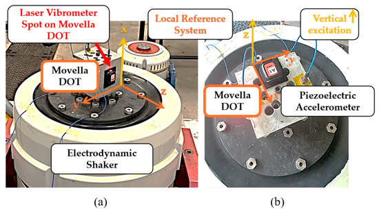
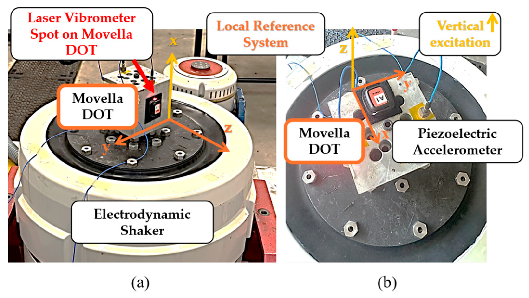
The experimental setup is illustrated in Figure 1. The Movella DOT to be assessed is mounted on a mechanical interface on an electrodynamic shaker (LDS V830, by Brüel & Kjær, Nærum, Denmark), as the controlled vibration source (acting along vertical direction Z), a piezoelectric reference accelerometer (PCB 333B30, with a nominal sensitivity of 10.2 mV/m/s², measurement range equal to ±490 m/s² pk, by PCB Piezoelectronics, Depew (NY), USA) for the controller, and a laser vibrometer (model OFV-5000 Xtra Laser Vibrometer, OFV-505 Sensor Head, by Polytec GmbH, Waldbronn, Germany) for acceleration acquisition and data comparison. The local reference system of the Movella DOT is reported. In the illustrated scenario, a Movella DOT (labelled as A1) was tested along the x-axis, aligned with the vertical direction Z. The sampling frequency of the laser vibrometer was fixed at 2048 Hz in order to verify any deviation from the nominal excitation frequency, while the Movella DOT was set at its maximum, i.e., 120 Hz. Throughout all test sessions, the excitation axis in the global reference system was kept fixed in the vertical direction. The Movella DOT sensors were mounted to receive mono-axial excitation (i.e., with their local axis parallel to the excitation axis), allowing each acceleration axis to be assessed individually, as shown in Figure 1.

Figure 1. The mechanical interface and sensing devices are mounted on the electrodynamic shaker, controlled via a piezoelectric accelerometer. The laser beam is aligned vertically with the Movella DOT sensor. The local reference frame (orange colour) and vertical excitation axis (yellow colour) are shown for: (a) Movella DOT x-direction testing, and (b) Movella DOT z-direction testing.

The experimental campaign was structured into seven distinct test sessions to systematically characterise the performance of four wearable sensors, as summarised in Table 1. The first batch comprises three identical units (A1, A2, and A3), while a fourth sensor (B1) was selected from a second batch to assess batch-to-batch reproducibility.

Table 1. Summary of the test session for Movella DOT sensors calibration.

Test Session Objective	Sensors	Excitation Type and Level *	Excitation Frequencies (Hz)	Accelerometer Axes	Acquisition and Processing Parameters
Repeatability and Reproducibility within a batch (#1)	A1	Stepped Sine (1 g)	5, 10, 18, 25, 30, 35, 38, 40, 42, 45	Monaxial (x-direction)	Sampling frequency: 120 Hz Spectral resolution: 0.1 Hz
	A2
	A3
Linearity vs. level variability within a batch (#2)	A1	Stepped Sine (1 g, 2 g, 3 g, 15 g)	5, 10, 18, 25, 30, 35, 38, 40, 42, 45	Monaxial (x-direction)	Sampling frequency: 120 Hz Spectral resolution: 0.1 Hz
	A2	Stepped Sine (1 g, 2 g, 3 g)
	A3
Directional variability (#3)	A1	Stepped Sine (1 g)	5, 10, 18, 25, 30, 35, 38, 40, 42, 45	Triaxial (y- and z-directions)	Sampling frequency: 120 Hz Spectral resolution: 0.1 Hz
Reproducibility between batches (#4)	B1	Stepped Sine (1 g)	5, 10, 18, 25, 30, 35, 38, 40, 42, 45	Monaxial (x-direction)	Sampling frequency: 120 Hz Spectral resolution: 0.1 Hz
Stability (#5)	A1	Stepped Sine (1 g)	10	Monaxial (x-direction)	Sampling frequency: 120 Hz Spectral resolution: 0.1 Hz
Aliasing conditions (#6)	A1	Stepped Sine (1 g)	70, 90, 110, 115, 117, 118, 119, 120, 121, 130, 140, 150, 160, 170, 175, 180, 185, 190, 195, 200, 220, 250, 255	Monaxial (x-direction)	Sampling frequency: 120 Hz Spectral resolution: 0.1 Hz
	A2
	A3
Dynamic Validation (#7)	A1	Random Profile (RMS: 1 g)	Bandwidth: [8–40] Hz	Monaxial (x-direction)	Sampling frequency: 120 Hz 100 spectral averages Spectral resolution: ≈ 0.17 Hz

* g is meant to be the gravitational acceleration, i.e., 9.81 m/s².

For test sessions #1 through #4, the excitation profile consisted of a stepped-sine wave at a fixed acceleration level (limited between 1 g and 15 g) and a discrete frequency. The procedure aimed to target the nominal sensor bandwidth, within the device’s bandwidth, applying excitation at specific frequencies, i.e., 5, 10, 18, 25, 30, 35, 38, 40, 42, and 45 Hz. In detail, the repeatability and reproducibility were assessed by test session #1, which investigated the performance of the three units of the primary batch (labelled respectively as A1, A2, and A3) under a nominal mono-axial excitation of 1 g (g is meant to be gravitational acceleration), for at least 1 min of excitation input for each trial. Here, the intra-sensor repeatability was assessed by comparing the sensors to three identical consecutive test trials under constant excitation conditions, as described in detail in Table 1. For each trial, continuous time-history data were recorded, from which three 1 min time windows were extracted for subsequent statistical analysis in the frequency domain.

This test session was followed by the linearity and level variability evaluation (session #2), where the linearity was evaluated with mono-axial harmonic excitation on sensor A1 across multiple levels (1 g, 2 g, 3 g, and 15 g) and on sensors A2 and A3 up to 3 g maximum sine amplitude. Moreover, the session also allowed the quantification of the inter-sensor and intra-batch reproducibility by comparing three separate sensors from the same production lot under an identical excitation level.

To assess the dynamic behaviour of the sensors across the tri-axes, the directional variability session (#3) was dedicated to additional testing of sensor A1 along its local y- and z-directions under a 1 g stepped-sine profile.

The reproducibility between batches was evaluated in test session #4 by comparing these baseline results against the secondary batch unit (i.e., sensor B1), under identical 1 g mono-axial conditions (x-direction). Short-term signal behaviour was instead evaluated during the stability check session (test session #5), which subjected sensor A1 to continuous operation at 1 g for 10 min. In order to verify the presence of an aliasing error, the three sensors A1, A2 and A3 were tested at frequencies (i.e., 70, 90, 110, and 130 Hz) higher than the Nyquist frequency. Concluding the procedure, test session #7 introduced a 10 min random excitation profile spanning a continuous 8 to 40 Hz bandwidth at an overall energy level of 1 g of RMS (Root Mean Square) input acceleration value. This latter session allowed for validation of the sensors’ behaviour with a limited-band dynamic signal.

2.3. Data Analysis Processing

2.3.1. FRF Moduli Evaluation

In order to characterise the FRF moduli in the analysed condition, the following steps were applied to the acquired time histories. As previously described, two independent acquisition systems were used for the vibrometer and the Movella DOT accelerometers, thus requiring the resampling of the vibrometer signal at the same sampling frequency (i.e., 120 Hz) as the Movella DOT sensors.

After resampling the laser vibrometer data, the frequency analyses of the Movella DOT accelerometer and the reference laser vibrometer data were evaluated by extracting the harmonic content from the acquired time series. Then, a 10 s time window was extracted for a single FFT evaluation (thus providing a spectral resolution of 0.1 Hz).

Furthermore, the transfer function of the sensor was characterised by computing the experimental Frequency Response Function (FRF, labelled as H_e) modulus, as shown in Equation (1), which was calculated as the direct ratio of the peak spectral amplitudes of the Movella DOT sensor (A_M) to the frequency-scaled acceleration amplitude spectrum of the vibrometer reference (labelled as A_v). Because the laser vibrometer measures point velocity rather than acceleration, frequency-domain differentiation was applied, which corresponds to multiplication by jω of the velocity amplitude spectrum V_v, where j is the imaginary unit, and ω is the angular frequency of the input:

$$\left|H_e\left(f\right)\right|={\displaystyle \frac{\max A_M\left(f\right)}{\max A_v\left(f\right)}}={\displaystyle \frac{\max A_M\left(f\right)}{\mathsf{\omega } \max V_v\left(f\right)}}$$

(1)

The modulus ratio was evaluated across all tested discrete frequencies to reconstruct the experimental modulus of the FRF, as well as for the aliased and stability conditions (test sessions #5 and #6).

The robustness of the obtained results was verified by computing the mean and standard deviation of the FRF modulus for each excitation frequency, considering three time histories of 15 s to be used for computing the FRF. Indeed, the metrics served to assess also the intra-sensor repeatability (A1), inter-sensor repeatability (A1, A2, and A3), consistency across various acceleration levels and directions, and reproducibility across distinct sensor batches (A1 vs. B1 comparison).

Then, to assess measurement stability, ten windows lasting 10 s each were extracted at 1 min intervals across the stability testing acquisition, lasting 10 min. The FRF amplitude was computed, and the system stability was quantified by evaluating the FRF’s variability.

2.3.2. FRF Optimisation

Using the first production batch dataset (i.e., Sensors A1, A2, and A3), a numerical optimisation was executed within the 5–55 Hz bandwidth to establish the sensor dynamic model. To account for high-frequency distortions, out-of-band aliased conditions (from 70 Hz to 130 Hz) were integrated into a secondary step of the evaluation. Because the experimental FRF data contained only amplitude values, the optimisation minimised the difference between the measured and numerical amplitudes to identify equivalent transfer-function models for the Movella DOT sensor. This approach would allow for recovering the phase, not measurable with the implemented approach, given the large uncertainty of the synchronisation between the vibrometer and the Movella DOT signals due to the limitation of the sampling rate of the Movella DOT. The optimisation problem is formulated by minimising the squared difference between the experimental and numerical transfer functions, as shown in Equation (2):

$$J\left(\theta \right)={\displaystyle {\sum }_{i=1}^N}{(\left|H_e\left({\omega }_i\right)\right|-\left|H_m\left({\omega }_i\right)\right|)}^2$$

(2)

where θ represents the model parameters, $\left|H_e\right|$ is the measured FRF amplitude, $\left|H_m\right|$ is the amplitude response of the fitted transfer function, and ω_i is the i-th considered angular frequency.

The optimisation problem was implemented in MATLAB R2025b using the lsqcurvefit function as a numerical solver, characterised by the trust-region reflective algorithm. Tight convergence tolerances and high iteration limits were used to improve convergence and reduce numerical fitting errors. In particular, the maximum number of iterations and function evaluations were both set to 20,000. The step tolerance was set to 10⁻¹⁴, while the function tolerance was set to 10⁻¹⁰. For the time-constant models, each time constant was constrained between 10⁻⁶ s and 10 s to prevent nonphysical or numerically ill-conditioned parameter estimates.

Two modelling strategies were considered. First, physically interpretable time-constant cascade models were developed using the dataset within the Nyquist frequency. These stable, low-pass filtering structures—ranging from first to third order—are defined in Equation (3), Equation (4) and Equation (5), respectively, where the time constants (${\tau }_i,$I = 1,.., 3) were the optimisation variables.

$$H_{m,1}\left(j\omega \right)={\displaystyle \frac{1}{({\tau }_{1}j\omega +1)}}$$

(3)

$$H_{m,2}\left(j\omega \right)={\displaystyle \frac{1}{({\tau }_{1}j\omega +1)({\tau }_{2}j\omega +1)}}$$

(4)

$$H_{m,3}\left(j\omega \right)={\displaystyle \frac{1}{({\tau }_{1}j\omega +1)({\tau }_{2}j\omega +1)({\tau }_{3}j\omega +1)}}$$

(5)

Furthermore, a higher-order general transfer function was modelled using the full dataset, including the results of the aliasing testing phase.

The numerical model of interest is shown in Equation (6), where the angular frequency variable is scaled to improve numerical stability (Equation (7)): ${\omega }_{max}$ is the maximum angular frequency in the fitted dataset, whereas q is the normalised angular frequency. The model utilised a sixth-order numerator and a seventh-order denominator.

$$H_{m,4}\left(jq\right)={\displaystyle \frac{b_6{\left(jq\right)}^6+b_5{\left(jq\right)}^5+b_4{\left(jq\right)}^4{+b}_3{\left(jq\right)}^3{+b}_2{\left(jq\right)}^2+b_1\left(jq\right)+b_0}{{{a_7\left(jq\right)}^7+a}_6{\left(jq\right)}^6+a_5{\left(jq\right)}^5+a_4{\left(jq\right)}^4{+a}_3{\left(jq\right)}^3{+a}_2{\left(jq\right)}^2+a_1\left(jq\right)+a_0}}$$

(6)

$$q={\displaystyle \frac{\omega }{{\omega }_{max}}}$$

(7)

The presented optimisation settings (i.e., maximum number of iterations, function evaluations, step tolerance, and function tolerance) were applied consistently to the first-, second-, and third-order time-constant models and to the general transfer-function model; then, the coefficients of the general transfer-function model were estimated without explicit lower or upper bounds.

Finally, to evaluate the accuracy of the numerical models, the residual Root Mean Square Error (RMSE) was computed based on the differences between the numerical predictions and the experimental dataset, within the instrument’s bandwidth.

2.3.3. PSD Measurement and FRF Model Validation

Random vibration data were processed using the previously described procedure, which first converts time-domain signals into the frequency domain via Fast Fourier Transform (FFT). Then, the Power Spectral Density (PSD) was determined by taking the ensemble average of these 100 power spectra and dividing by the frequency bandwidth. Furthermore, to evaluate the performance of the data acquisition system, the numerical models derived from the calibration phase were applied directly to the Movella DOT’s PSD, according to the linear system relation [34]:

$${PSD}_c={PSD}_e/{\left|H_{m,i}\right|}^2$$

(8)

where H_m,i is the i-th modelled FRF, as in Section 2.3.2, and PSD_e is the measured PSD by the Movella DOT sensor.

The resulting corrected PSDs (PSD_c) were then compared to the experimental PSD_v extracted from the vibrometer. Finally, the discrepancy between the vibrometer and corrected data from the Movella DOT was quantified by calculating the mean PSD values and their standard deviations across the reference, uncorrected, and corrected signals.

Hence, the objective of this analysis is to compensate for the limited measurement bandwidth of the Movella DOT sensor by using a reference vibrometer to validate a dynamic correction model, thereby restoring the underestimated PSD to its correct values.

3. Results

3.1. FRFs Repeatability, Reproducibility and Linearity

In this section, the measured FRFs are shown, presenting the repeatability, reproducibility, variability in the measurement directions and non-linearity analyses.

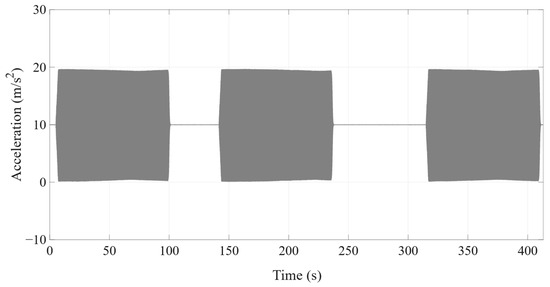
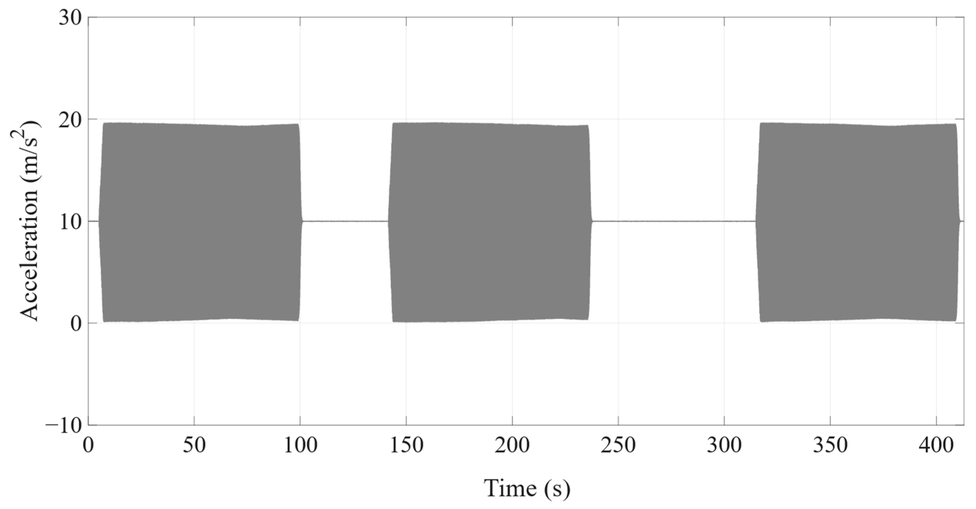
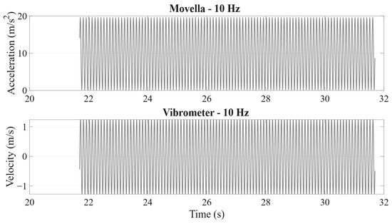
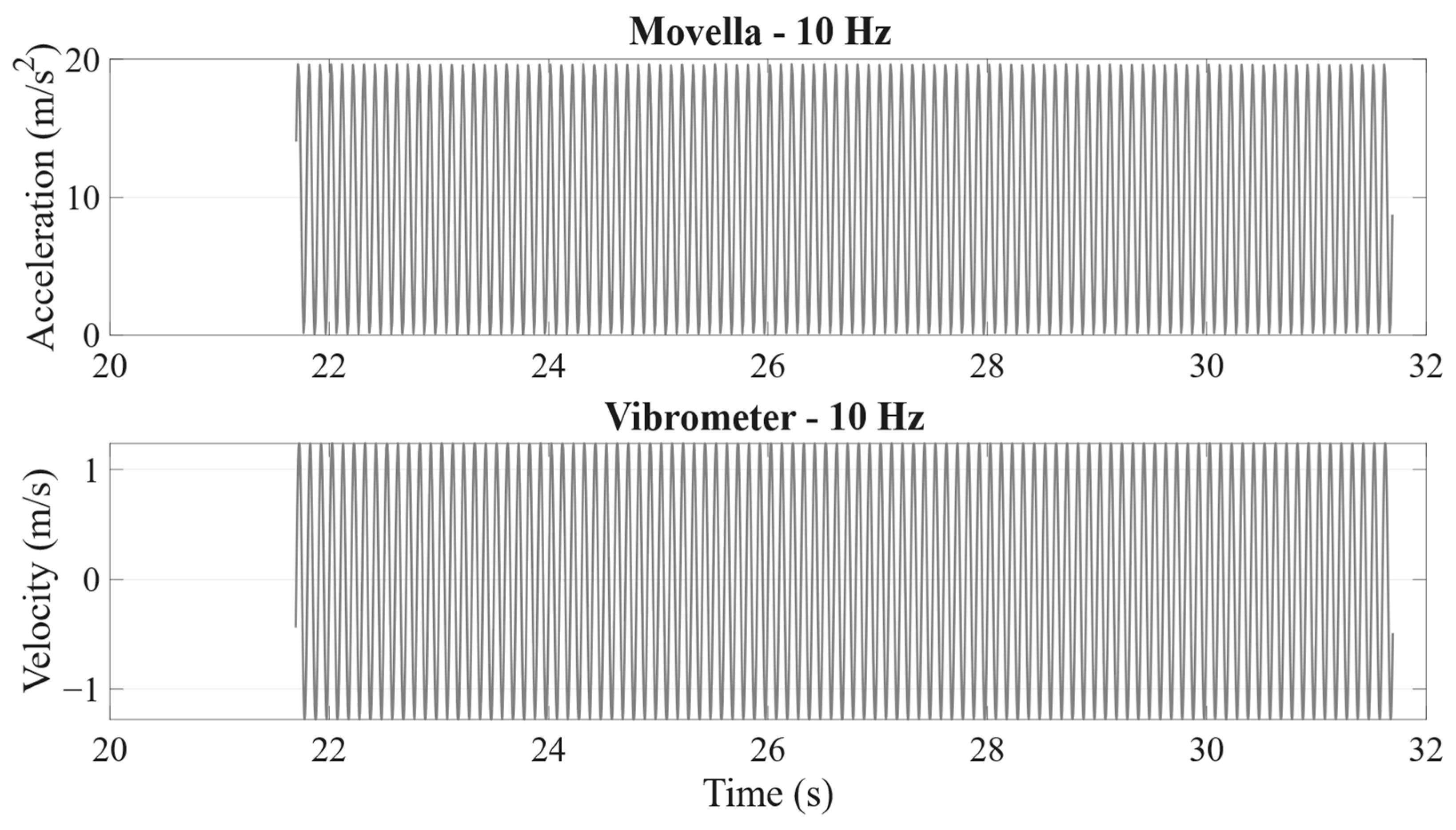
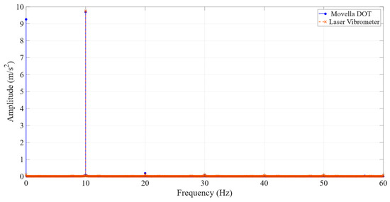
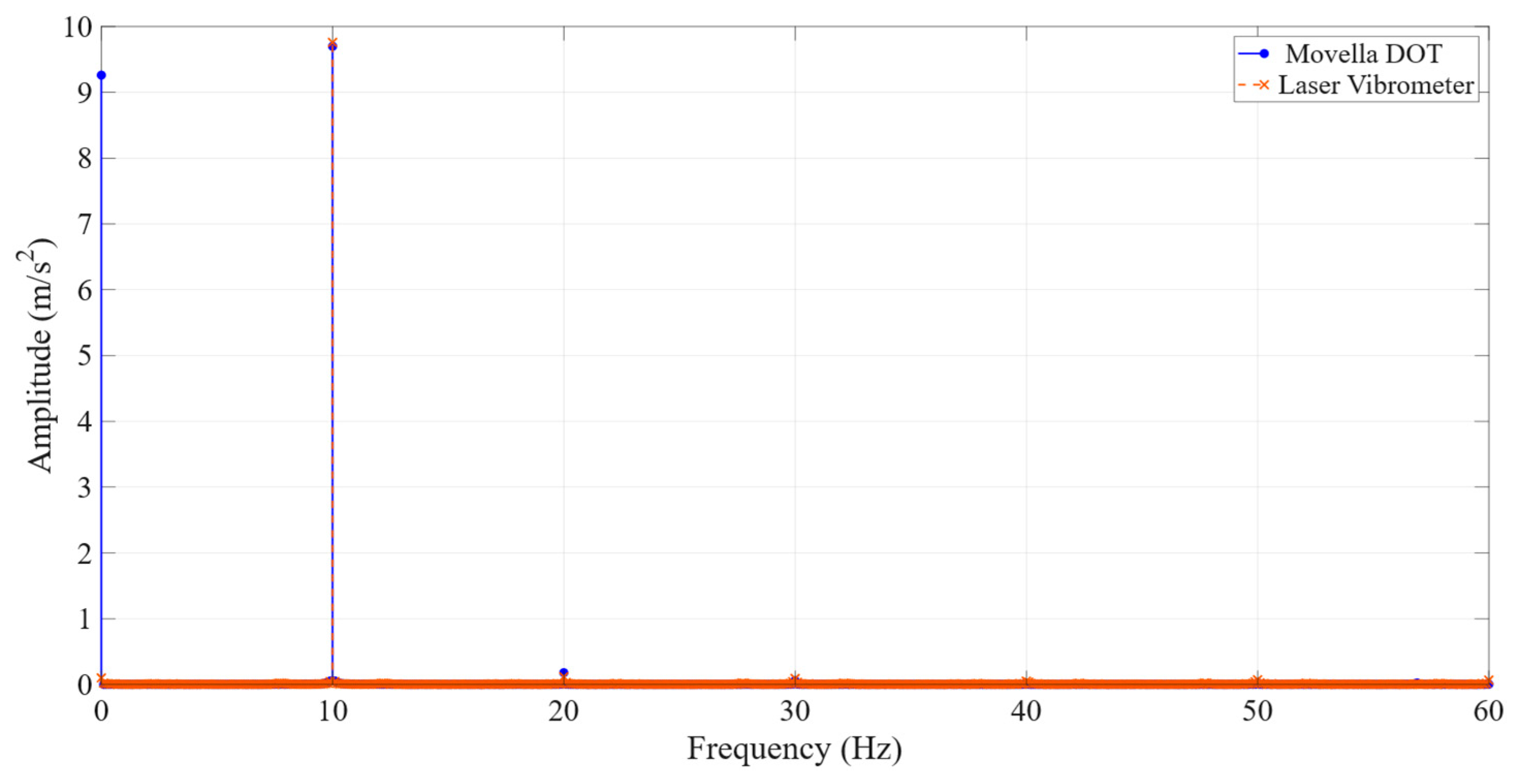
Figure 2 shows the measured acceleration by sensor A1, considering three subsequent tests: in particular, the graph shows the accelerometer response at 1 g excitation level and 10 Hz frequency, along the x-direction. Figure 3 shows an example of the 10 s time windows for the spectrum computation for the accelerometer A1, whereas Figure 4 summarises the spectra of the accelerometer and of the vibrometer for the selected time window.

Figure 2. Time-domain signal: example of three datasets in sequence acquired for sensor A1, with a stepped sine excitation (level: 1 g, frequency: 10 Hz, x-direction). Sampling frequency: 120 Hz.

Figure 3. Example of a 10 s time window for spectral analysis: sensor A1, 1 g level, 10 Hz.

Figure 4. Frequency domain: example FFT magnitude for sensor A1, with a stepped sine excitation (level: 1 g, frequency: 10 Hz, x-direction). Sampling frequency: 120 Hz. A static component is present, representing the gravitational acceleration, with the excitation component at 10 Hz. In blue and orange colours are shown the measured spectra for the Movella DOT and Laser Vibrometer, respectively.

The measured FRF amplitude $\left|H_e\left(f\right)\right|$ for each tested input frequency is shown in Table 2 for sensor A1, tested along the x-direction. In addition, the mean values and the standard deviation (1σ), expressed as a percentage, were calculated from three different windows selected from three independent but consecutive experiments, as shown in Figure 2 and presented below. Table 3 and Table 4 present the measured values for sensors A2 and A3, respectively.

Table 2. FRF evaluation of three time windows (A1 sensor), 1 g level, sine-step along the x-direction.

Frequency (Hz)	$\left|{\mathit{H}}_{\mathit{e}}\left(\mathit{f}\right)\right|$
	Window 1	Window 2	Window 3	Mean Value	1σ (%)
5	0.9958	0.9957	0.9955	0.9957	<0.05%
10	0.9866	0.9866	0.9862	0.9865	<0.05%
18	0.9594	0.9593	0.9593	0.9593	<0.05%
25	0.9238	0.9237	0.9239	0.9238	<0.05%
30	0.8924	0.8922	0.8921	0.8922	<0.05%
35	0.8556	0.8556	0.8557	0.8556	<0.05%
38	0.8317	0.8317	0.8317	0.8317	<0.05%
40	0.8148	0.8149	0.8145	0.8147	0.08%
42	0.7972	0.7971	0.7972	0.7971	<0.05%
45	0.7699	0.7698	0.7697	0.7698	<0.05%

Table 3. FRF evaluation of three time windows (A2 sensor), 1 g level, sine-step along the x-direction.

Frequency (Hz)	$\left|{\mathit{H}}_{\mathit{e}}\left(\mathit{f}\right)\right|$
	Window 1	Window 2	Window 3	Mean Value	1σ (%)
5	0.9982	0.9998	0.9994	0.9991	0.08%
10	0.9947	0.9872	0.9874	0.9898	0.43%
18	0.9605	0.9604	0.9605	0.9604	<0.05%
25	0.9251	0.9251	0.9252	0.9251	<0.05%
30	0.8936	0.8940	0.8937	0.8938	<0.05%
35	0.8572	0.8570	0.8573	0.8572	<0.05%
38	0.8332	0.8330	0.8331	0.8331	<0.05%
40	0.8152	0.8153	0.8151	0.8152	<0.05%
42	0.7982	0.7981	0.7980	0.7981	<0.05%
45	0.7707	0.7705	0.7706	0.7706	<0.05%

Table 4. FRF evaluation of three time windows (A3 sensor), 1 g level, sine-step along the x-direction.

Frequency (Hz)	$\left|{\mathit{H}}_{\mathit{e}}\left(\mathit{f}\right)\right|$
	Window 1	Window 2	Window 3	Mean Value	1σ (%)
5	0.9974	0.9983	0.9974	0.9977	0.06%
10	0.9876	0.9874	0.9873	0.9874	<0.05%
18	0.9605	0.9603	0.9603	0.9604	<0.05%
25	0.9250	0.9250	0.9249	0.9250	<0.05%
30	0.8930	0.8931	0.8931	0.8931	<0.05%
35	0.8563	0.8565	0.8564	0.8564	<0.05%
38	0.8325	0.8327	0.8325	0.8326	<0.05%
40	0.8163	0.8154	0.8147	0.8155	0.10%
42	0.7981	0.7979	0.7979	0.7979	<0.05%
45	0.7708	0.7709	0.7709	0.7709	<0.05%

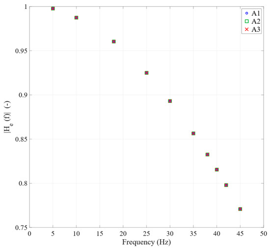
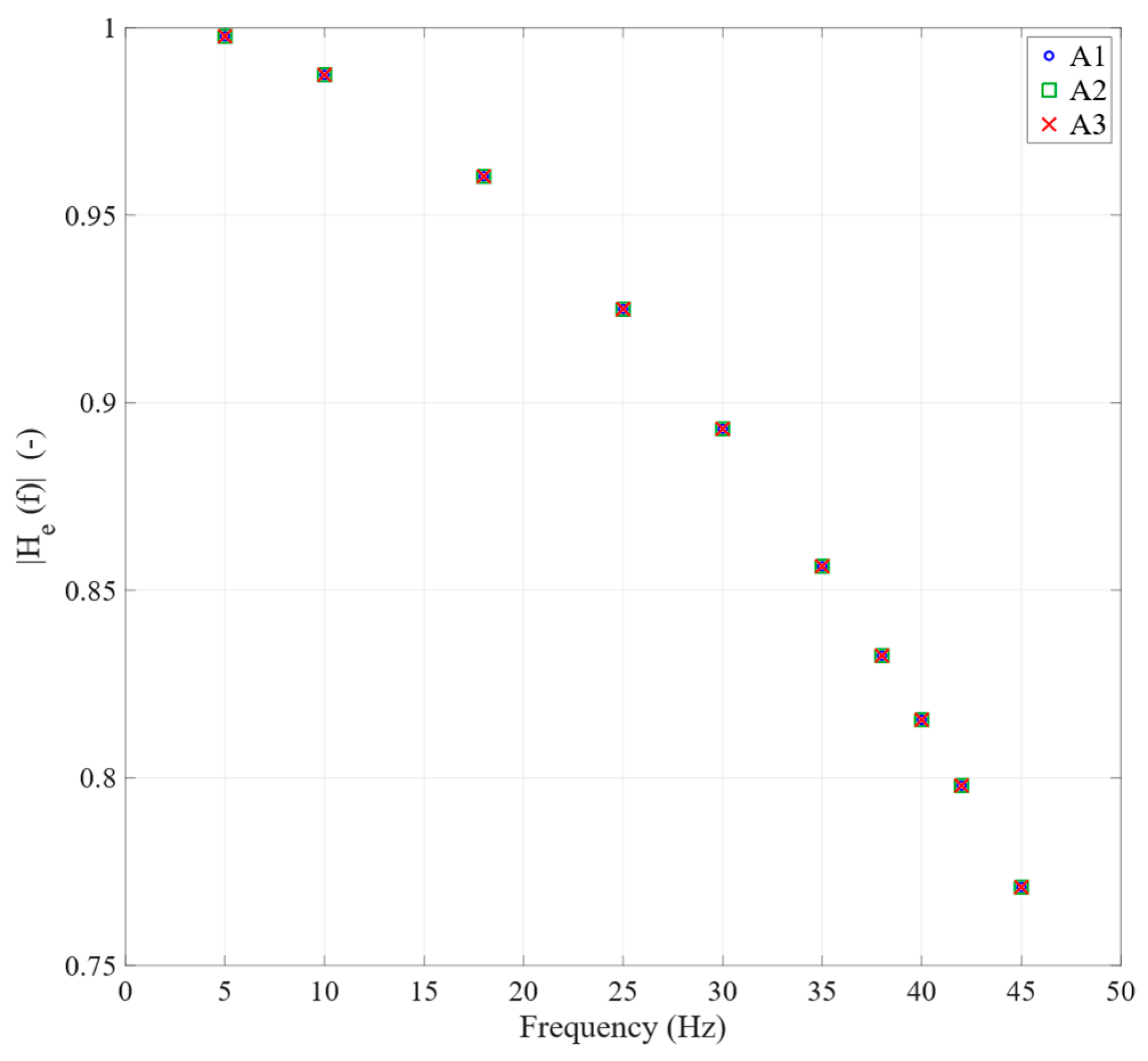
For sensor-to-sensor reproducibility, the measured FRF amplitudes and the corresponding coefficients of variation across the three sensors are reported in Table 5. Then, the moduli of the presented FRFs are shown in the frequency domain, illustrated in Figure 5.

Table 5. FRF estimation of three sensors (A1, A2 and A3), 1 g level, sine-step along the x-direction.

Frequency (Hz)	$\left|{\mathit{H}}_{\mathit{e}}\left(\mathit{f}\right)\right|$
	A1	A2	A3	Mean Value	1σ (%)
5	0.9957	0.9991	0.9977	0.9975	0.17%
10	0.9865	0.9898	0.9874	0.9879	0.17%
18	0.9593	0.9604	0.9604	0.9600	0.07%
25	0.9238	0.9251	0.9250	0.9246	0.08%
30	0.8922	0.8938	0.8931	0.8930	0.09%
35	0.8556	0.8572	0.8564	0.8564	0.09%
38	0.8317	0.8331	0.8326	0.8325	0.09%
40	0.8147	0.8152	0.8155	0.8151	0.05%
42	0.7971	0.7981	0.7979	0.7977	0.06%
45	0.7698	0.7706	0.7709	0.7704	0.07%

Figure 5. FRF moduli of three sensors represented in the frequency domain. Values for three sensors A1, A2 and A3, under 1 g level, sine-step along the x-direction.

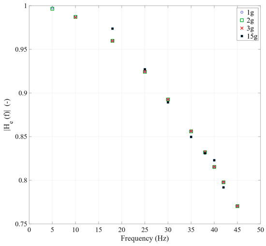
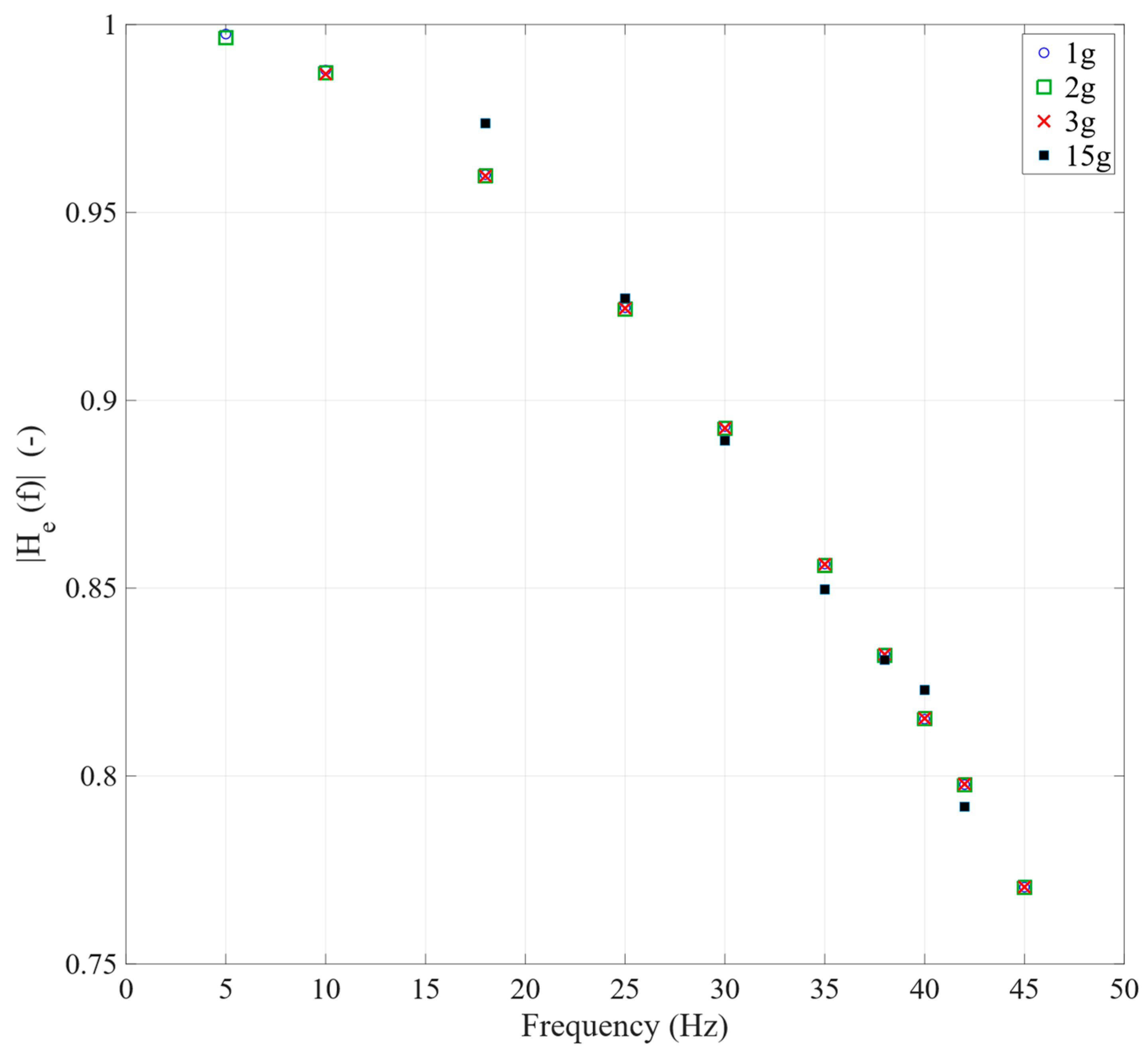
Linearity (test session #2) was assessed by considering the effect of the excitation amplitude. Table 6 reports the FRF repeatability results for the three sensors under the 1 g, 2 g, and 3 g excitation levels. The 15 g scenario was included to assess the sensor behaviour close to its upper measurement range (FS), and the corresponding results are also reported below. In addition, the moduli of the presented FRFs are shown in the frequency domain plot in Figure 6. For the 15 g test case, 5 Hz and 10 Hz excitations were omitted due to the displacement limits of the shaker, while the data for the 45 Hz excitation were corrupted. Nevertheless, these missing data points do not compromise the overall validity of the analysis. To further assess the linearity of the instrument response, the maximum absolute relative difference (Δmax) between the measured average FRF amplitudes and the data points collected at each frequency was computed.

Table 6. FRF estimation of four different amplitudes (1 g, 2 g, 3 g, 15 g) for A1, testing in the x-direction, sine-step excitation, A1 sensor.

Frequency (Hz)	$\left|{\mathit{H}}_{\mathit{e}}\left(\mathit{f}\right)\right|$
	1 g	2 g	3 g	15 g	Mean Value	1σ (%)	Δmax (%)
5	0.9957	0.9958	-	-	0.9958	<0.05%	0.005%
10	0.9865	0.9875	0.9872	-	0.9871	0.05%	0.057%
18	0.9593	0.9594	0.9594	0.9737	0.9630	0.74%	1.1%
25	0.9238	0.9239	0.9240	0.9271	0.9247	0.17%	0.26%
30	0.8922	0.8918	0.8921	0.8893	0.8914	0.15%	0.23%
35	0.8556	0.8556	0.8558	0.8497	0.8542	0.35%	0.52%
38	0.8317	0.8317	0.8317	0.8309	0.8315	0.05%	0.072%
40	0.8147	0.8145	0.8144	0.8229	0.8166	0.51%	0.77%
42	0.7971	0.7970	0.7972	0.7918	0.7958	0.33%	0.50%
45	0.7698	0.7698	0.7699	-	0.7698	<0.05%	0.009%

Figure 6. FRF amplitude responses at 1 g, 2 g, 3 g and 15 g.

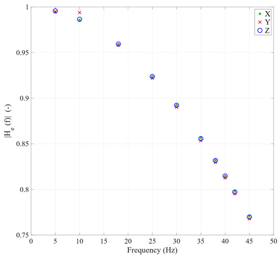
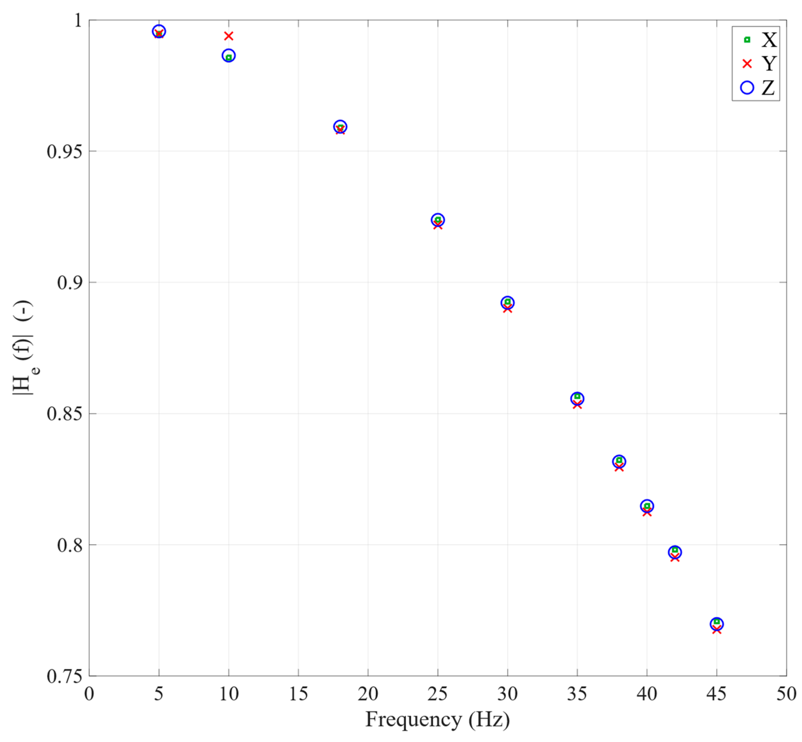
Repeatability along the different measurement directions (test session #3 of the testing protocol) was performed by fixing the excitation amplitude and using sensor A1 to evaluate the FRF responses. The results are collected in Table 7. Figure 7 illustrates the experimental FRFs for testing session #3.

Table 7. FRF evaluation of A1, testing in x-, y- and z-directions, 1 g sine-step excitation.

Frequency (Hz)	$\left|{\mathit{H}}_{\mathit{e}}\left(\mathit{f}\right)\right|$
	x	y	z	Mean Value	1σ (%)
5	0.9957	0.9949	0.9947	0.9951	0.05%
10	0.9865	0.9856	0.9939	0.9887	0.46%
18	0.9593	0.9590	0.9581	0.9588	0.07%
25	0.9238	0.9240	0.9219	0.9232	0.13%
30	0.8922	0.8924	0.8901	0.8916	0.14%
35	0.8556	0.8563	0.8535	0.8551	0.17%
38	0.8317	0.8322	0.8296	0.8312	0.17%
40	0.8147	0.8147	0.8125	0.8140	0.16%
42	0.7971	0.7982	0.7952	0.7968	0.19%
45	0.7698	0.7708	0.7677	0.7694	0.21%

Figure 7. FRF amplitude responses at 1 g, in all the tested directions (x, y and z).

To further evaluate the manufacturing reproducibility, sensors from different production batches were tested under the same excitation condition.

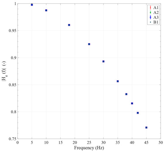
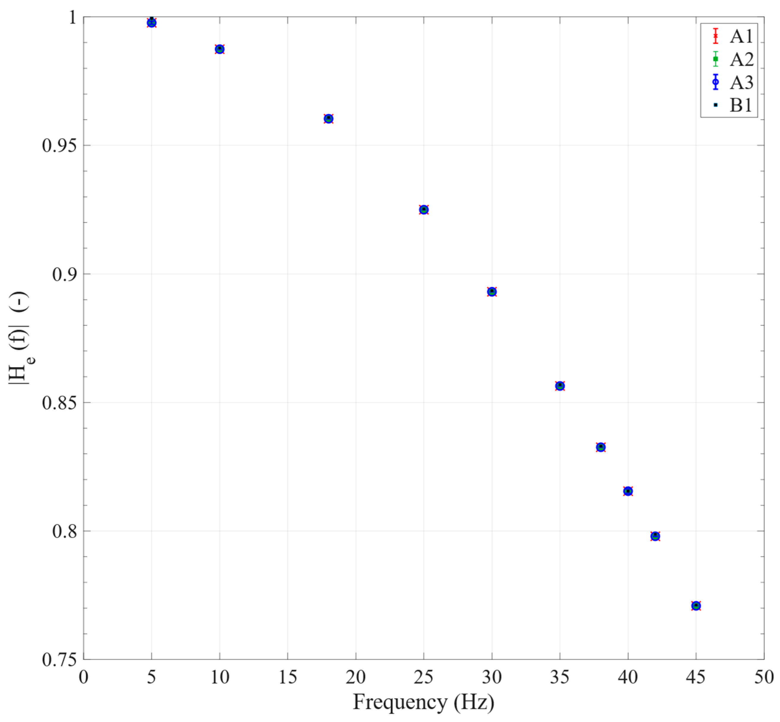
Results of the testing session #4, in which sensors from different batches were compared, are summarised in Table 8. Figure 8 shows the related experimental FRFs.

Table 8. FRF estimation of B1 with comparison with the average of the other sensors (A1, A2, A3), testing in the x-direction, 1 g sine-step excitation.

Frequency (Hz)	$\left|{\mathit{H}}_{\mathit{e}}\left(\mathit{f}\right)\right|$
	A	B1	Mean Value	1σ (%)
5	0.9975	0.9994	0.9985	0.20%
10	0.9879	0.9879	0.9879	<0.05%
18	0.9600	0.9609	0.9604	0.08%
25	0.9246	0.9253	0.9250	0.07%
30	0.8930	0.8934	0.8933	0.06%
35	0.8564	0.8569	0.8567	0.06%
38	0.8325	0.8330	0.8327	0.05%
40	0.8151	0.8155	0.8153	<0.05%
42	0.7977	0.7987	0.7982	0.11%
45	0.7704	0.7712	0.7708	0.11%

Figure 8. Batch-to-batch FRF comparison using sensors from different production batches, 1 g level; 1σ error bars are shown for A1, A2 and A3 sensors.

3.2. Sensor Stability

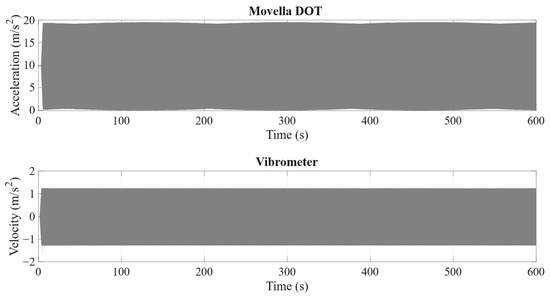
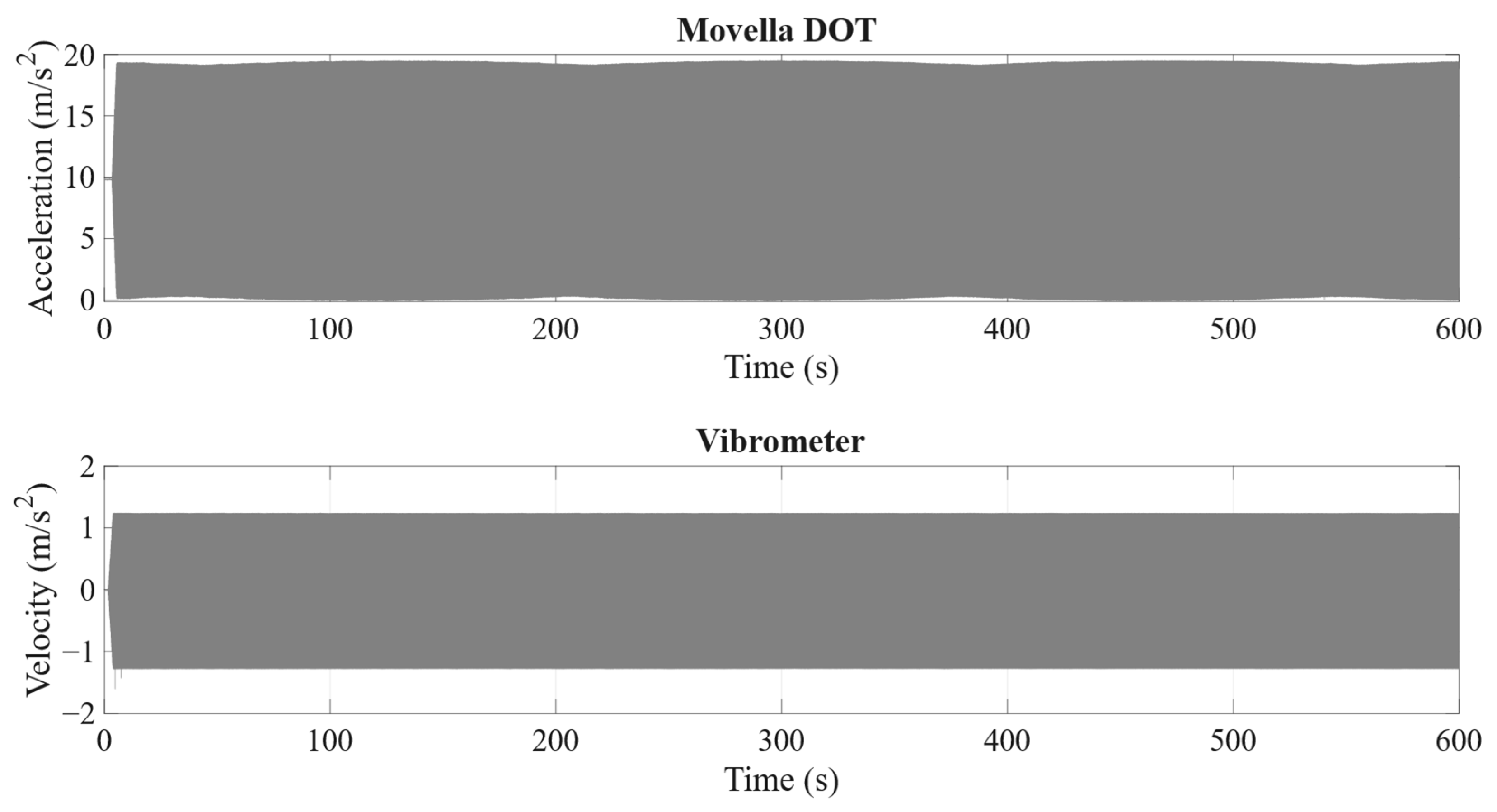
For the stability assessment, a 10 min acquisition was performed at 10 Hz using both the Movella DOT sensor and the laser vibrometer. As shown in Figure 9, both signals remained highly consistent over the 600 s duration with no visible amplitude drift. As summarised below (Table 9), the FFT peak amplitudes for both sensors exhibit negligible fluctuations across the ten intervals. The resulting FRF amplitudes maintain a stable average of 0.986, yielding a coefficient of variation of 0.019%, which satisfies the <0.05% stability threshold.

Figure 9. The raw data from the laser vibrometer and Movella DOT (A1) were acquired during continuous testing.

Table 9. Evaluation of short-term stability over time: experimental results for configuration A1 at a reference frequency of 10 Hz and 1 g acceleration level.

Time Windows	|AM| (m/s2)	|Av| (m/s2)	$\left|{\mathit{H}}_{\mathit{e}}\left(\mathit{f}\right)\right|$
1	9.7293	9.8712	0.9856
2	9.7330	9.8719	0.9859
3	9.7341	9.8709	0.9861
4	9.7310	9.8703	0.9859
5	9.7327	9.8710	0.9860
6	9.7324	9.8710	0.9860
7	9.7311	9.8707	0.9859
8	9.7335	9.8711	0.9861
9	9.7358	9.8707	0.9863
10	9.7317	9.8713	0.9859

3.3. Acquisition in Aliased Conditions

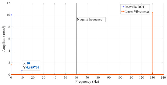
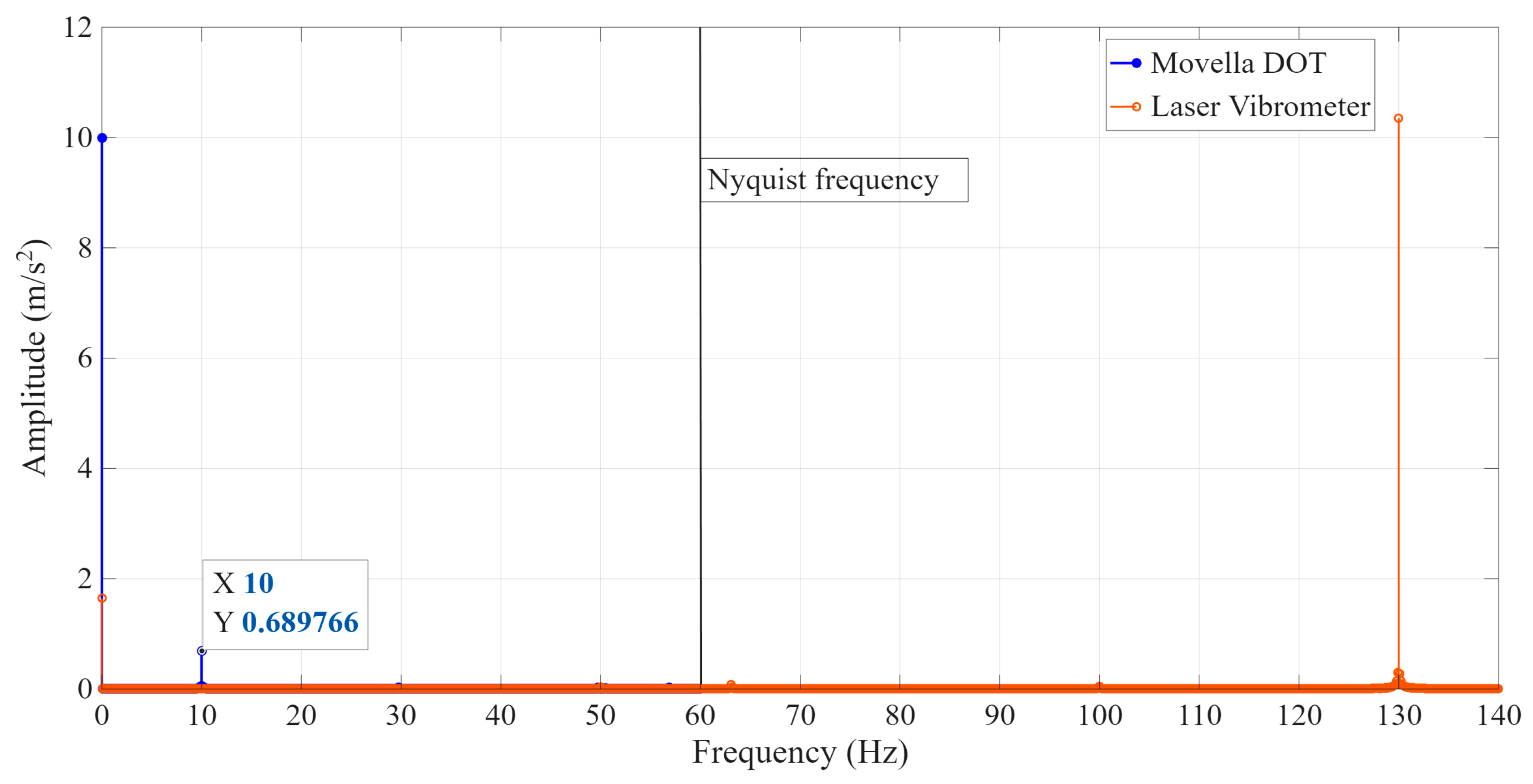
Frequency domain analyses were also performed to investigate the aliasing behaviour. The sensor was subjected to stepped-sine excitation at nominal frequencies ranging from 70 to 255 Hz (as defined in Table 1), with each test condition repeated three times. However, test repeatability was not available for excitation frequencies exceeding 170 Hz. Figure 10 shows a representative amplitude spectrum with $130\mathrm{Hz}$ excitation. Since the IMU samples at $120\mathrm{Hz}$ (Nyquist frequency of $60\mathrm{Hz}$), the $130\mathrm{Hz}$ signal is folded back and appears as an aliased peak at $10\mathrm{Hz}$. The spectrum of the Movella DOT also displays a static component (i.e., gravity acceleration), as for the previous acquisitions.

Figure 10. Spectra comparison (vibrometer vs. Movella DOT) for 130 Hz real excitation, A1 sensor, 1 g. The Nyquist frequency is highlighted with black solid vertical line.

All the computed Frequency Response Function (FRF) values are summarised in Table 10.

Table 10. FRF evaluation of A1 tested in aliasing conditions, testing in the x-direction, 1 g sine-step excitation.

Frequency (Hz)	$\left|{\mathit{H}}_{\mathit{e}}\left(\mathit{f}\right)\right|$
	Mean Value	1σ (%) *
70	0.5049	0.16%
90	0.2802	<0.05%
110	0.0810	0.07%
115	0.0391	0.27%
117	0.0230	0.17%
118	0.0036	3.30%
119	0.0033	4.19%
120	0.0040	22.96%
121	0.0029	1.62%
130	0.0665	<0.05%
140	0.1161	0.73%
150	0.1492	0.01%
160	0.1667	0.03%
170	0.1741	n.a.
175	0.1723	n.a.
180	0.2541	n.a.
185	0.1585	n.a.
190	0.1475	n.a.
195	0.1360	n.a.
200	0.1225	n.a.
220	0.0608	n.a.
250	0.0243	n.a.
255	0.0345	n.a.

* n.a. means that a measured standard deviation is not available.

3.4. FRF Optimisation Results

Table 11 collects the identified time constants, corresponding cutoff frequencies, and RMSE values for the three models, computed by means of the experimental dataset of FRF amplitudes within the sensor’s bandwidth. Table 12 shows the coefficients of the general transfer function.

Table 11. Optimisation result: numerical modelling on |FRF| bandwidth dataset.

Model	${\mathit{\tau }}_1\left[\mathit{m}\mathit{s}\right]$	${\mathit{\tau }}_2\left[\mathit{m}\mathit{s}\right]$	${\mathit{\tau }}_3\left[\mathit{m}\mathit{s}\right]$	RMSE
1st-order	2.8213	—	—	0.00825
2nd-order	1.8951	1.8952	—	0.00495
3rd-order	1.3146	1.3312	1.8696	0.00402

Table 12. General transfer-function optimisation results obtained by adding the aliased dataset. Coefficients are referred to in Equation (6).

Coefficient Order	$\mathit{a}$ Coefficients	$\mathit{b}$ Coefficients *
7	1.00	n.a.
6	−39,904.57	−1432.10
5	-97.70	7477.87
4	−13,054.98	−2112.16
3	−6596.75	9501.25
2	−6483.37	598.73
1	−684.06	1727.94
0	223.02	222.26
RMSE	0.00194

* n.a. means that a measured standard deviation is not available.

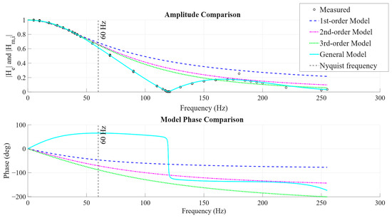
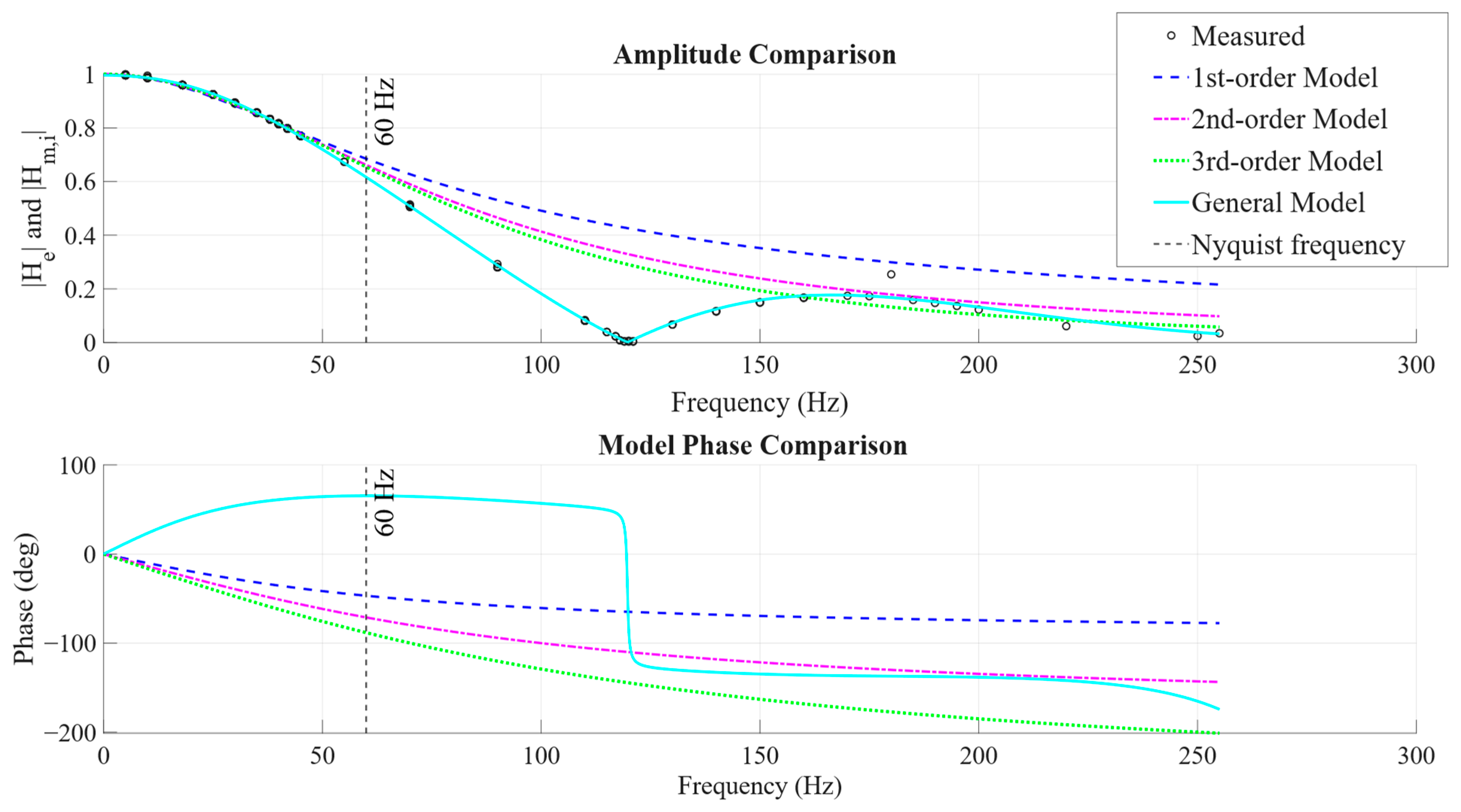
Figure 11 compares the measured FRF amplitude with the fitted time-constant models and the general transfer function. It should be noted that the amplitude data, represented by the experimental points, were used as input for the optimisation of the numerical models, from which the corresponding phase response was subsequently derived.

Figure 11. Amplitude and model-inferred phase responses of the fitted transfer-function models.

3.5. Random Excitation Results

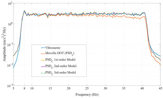
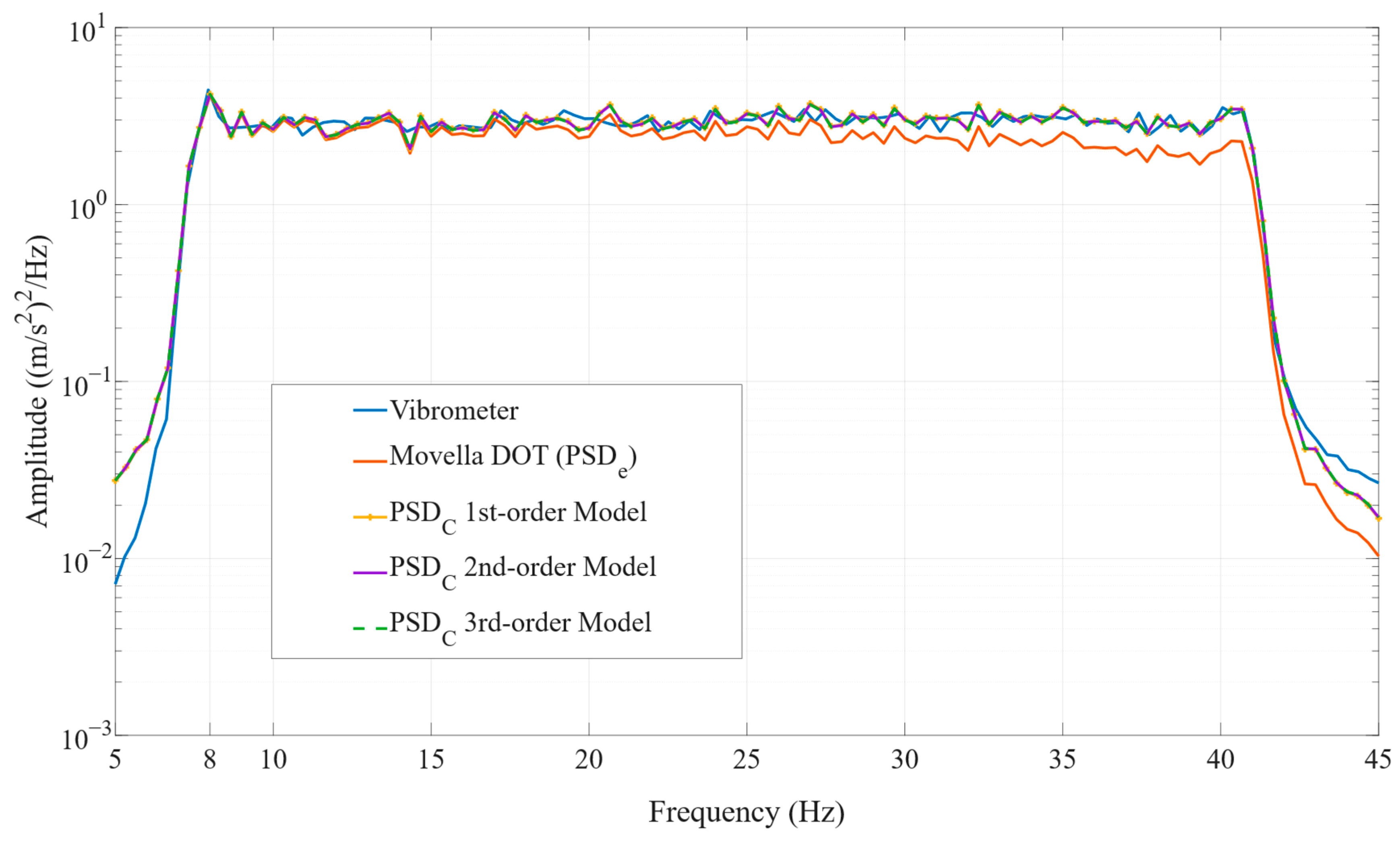
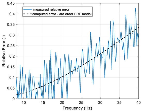
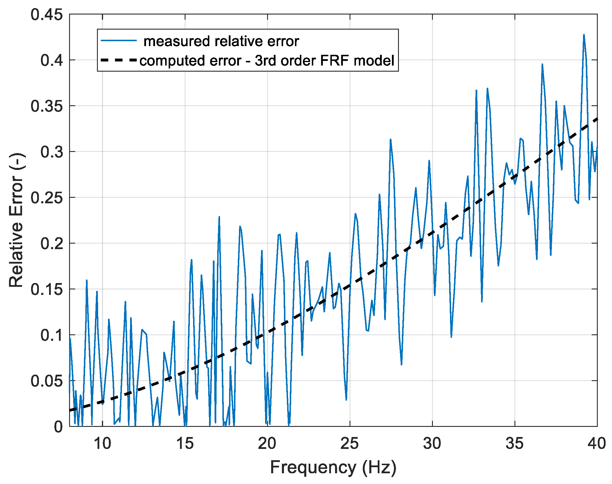
Figure 12 illustrates the experimental Power Spectral Densities (PSDs) of the reference laser vibrometer (PSD_v) and the Movella DOT sensor (PSD_e) under a 1 g RMS random excitation, compared against the corrected responses (PSD_c) obtained by using the models extracted from the experimental results. Figure 13 shows the relative error between the PSDv and PSDe, varying the excitation frequency and the computed numerical error considering the FRF amplitude of the third-order model.

Figure 12. Experimental and modelled PSD comparison under 1 g RMS random excitation: validation of first-, second-, and third-order numerical compensation filters against the reference laser vibrometer (PSD_v) and the Movella DOT sensor (PSD_e).

Figure 13. Relative error between vibrometer and uncorrected Movella DOT PSDs vs. frequency; dashed black line shows the computed error considering the FRF amplitude with a 3rd-order model.

Furthermore, the PSD of each signal was compared against the reference vibrometer PSD_v. The resulting statistics (mean values and standard deviations) within the 8–40 Hz bandwidth are summarised in Table 13. Here, the fifth column compares the uncorrected Movella (${\mathit{PSD}}_e$) and corrected (${\mathit{PSD}}_c$) values against the reference (${\mathit{PSD}}_v$), showing the percentage deviation from the reference.

Table 13. Comparison between the reference laser vibrometer and the Movella DOT sensor outputs (uncorrected vs. corrected via the models of first, second, and third order) in the 8–40 Hz frequency range.

Evaluated PSD	Mean Value ((m/s2)2/Hz)	1σ ((m/s2)2/Hz)	1σ (%)	Deviation from Reference (%)
Laser Vibrometer	2.957	0.274	9%	-
Movella DOT	2.491	0.322	13%	−15.76%
First-Order Model	2.980	0.268	9%	+0.78%
Second-Order Model	2.961	0.264	9%	+0.14%
Third-Order Model	2.956	0.263	9%	−0.03%

4. Discussion

The calibration protocol, based on comparing the Movella DOT against the laser vibrometer reference by computing the FRF amplitude, serves to characterise the dynamic response of the tested devices. The experimental results demonstrate, in general, strong repeatability and reproducibility across the amplitudes of the Frequency Response Functions (FRFs), providing a robust dataset for modelling the dynamic behaviour of the Movella DOT. In particular, the computed FRF amplitudes in the repeatability assessment showed a worst-case standard deviation of less than 0.1%, as summarised in Table 2, Table 3 and Table 4 for three sensors of the same batch (A1, A2 and A3, respectively).

Considering the variability between the sensors (as shown in Table 5), the obtained repeatability showed a worst-case standard deviation limited to 0.2%, validating the consistency of the measured dynamic response. The measured trends for the three tested accelerometers are shown in Figure 5: the general trend of the FRF amplitudes shows a reduction of about 23% near the Nyquist limit, highlighting the need for a dynamic correction for accurate dynamic measurements. Similar trends were found in the literature studies focusing on MEMS dynamic calibration [3,34,35].

The sensor linearity was verified by testing at different excitation levels. Indeed, as shown in Table 6, the measured FRFs provide repeatable trends (as depicted in Figure 6), with a worst-case standard deviation limited to about 0.74%. As shown in Table 6, the maximum relative error between the average FRF amplitude and the measured FRF values for each excitation level remained below approximately 1.1% (worst-case result at 18 Hz) across the investigated frequency range, without a systematic trend associated with the increasing excitation amplitude; this allows for supporting the linear behaviour of the instrument at the different excitation levels.

Cross-axis evaluation confirmed the directional consistency with a maximum variation of 0.2% between the accelerometer triaxial directions (as shown in Table 7). The variability observed across the three measurement directions remains limited (approximately to the worst-case value of 0.46%). It has to be noted that similar variability was observed at low frequencies in other cases (e.g., as shown in Table 3 and Table 6), suggesting that the variability is primarily associated with the intrinsic sensor response rather than with the measurement direction.

Moreover, the general reduction trend was confirmed, as shown in Figure 7, where the three FRFs are shown. Batch-to-batch repeatability was supported by the comparison between tested batches (shown in Figure 8 and Table 8), which showed worst-case variability limited to 0.2%, noting that the second batch was represented by just a single sensor. Eventually, the sensor stability was confirmed by the dedicated testing session, as shown in Figure 9 and summarised by Table 9: indeed, negligible variability was found (1σ % less than 0.02%), confirming the stability of the sensor for the tested time, i.e., 10 min.

The evaluation, initially conducted within the standard sensor bandwidth, was extended into aliased conditions to characterise the attenuation profile of higher-frequency components: although the devices’ dynamic response limits aliasing effects, signals above the Nyquist limit result in aliased components. This is quite evident when analysing the measured spectra shown in Figure 10, where the reference spectra (measured by the vibrometer) show the given input, whereas the signal measured in the aliased condition by the tested sensors shows an amplitude reduction and an apparent frequency symmetrised with respect to the Nyquist frequency. This is a limitation for the dynamic behaviour of the sensor, because in the case that the bandwidth of the measured signal cannot be controlled, the spectral measurements are corrupted by the aliasing error. The aliasing results agree with the FRF evaluation shown so far, as summarised by Table 10: in fact, the decreasing trend is confirmed, with a reduction of about 97% of the amplitude at 130 Hz. The data highlight a progressive attenuation of the sensor’s response as the frequency increases from 70 Hz to 120 Hz, where the mean FRF reaches a minimum value of 0.004. It can be noticed that the amplitude never drops to a true null value under any tested condition; as the FRF amplitude approaches the system’s noise floor (computed to be about 0.023 m/s²), the signal-to-noise ratio degrades (about 2.2 at 120 Hz), resulting in an increase in the measurement uncertainty to about 23%, therefore justifying the increased variability at that frequency and the impossibility of measuring a zero response as output of the sensor.

Regarding the numerical modelling of the sensor’s dynamic behaviour, the optimisation results showed that the first-order model captured the general low-pass trend of the measured FRF but showed higher discrepancies in the transition region due to sharper attenuation. Introducing an additional dynamic contribution (τ₂) in the second-order model enhanced the agreement with experimental data. The third-order model achieved the highest fidelity among the time-constant models, reducing the RMSE by approximately 50% compared to the first-order model (as shown in Table 11). The general transfer function model, whose coefficients are shown in Table 12, has the best performance, providing an overall RMSE which is the minimum among all the models. Indeed, the obtained reduction with the first-order modelling is about 90%.

Below 60 Hz, the time-constant models showed good agreement with the measured response, highlighting that the sensor behaviour within its bandwidth can be represented by a low-pass filter, as shown in similar devices [4]. When the full frequency range was considered, extending the analysis to the aliasing condition, the general transfer function provided the best global fitting performance, as also highlighted by the discrepancy in Figure 11 between the time-constant models and the experimental FRF amplitudes. Above 120 Hz, the FRF amplitude shows fluctuations which are fitted by the general model and are presumably caused by the implementation of the low-pass filter strategy (either numerical or hardware-based) by the sensor manufacturer. This confirmed the choice of selecting, among the models, a high-order filter to capture especially the FRF amplitude reduction between Nyquist and sampling frequencies, not properly captured even by increasing the order of the time-constant models above the used third order.

As mentioned before, the FRF modelling also provides the identification of the phase shift given by the device, allowing full dynamic correction. In Figure 11, the phase of all three time-constant models decreases monotonically. In contrast, the general model introduces an opposite trend, with a phase change near 120 Hz, corresponding to a theoretical null amplitude of the Movella DOT FRF. Indeed, the obtained results should be validated experimentally, solving the synchronisation issue between the two instruments, i.e., the Movella DOT and the laser vibrometer. Considering the general amplitude trend of the device (i.e., similar to a low-pass filtering for the FRF amplitude), it is suggested to use the phase trend of the time-constant models, assuming a general time delay between input and output.

Eventually, random testing showed that when the measured input is within the bandwidth of the sensors, the vibration signal is properly recovered if the proposed dynamic correction procedure, based on the modelled FRFs, is implemented. The latter finding is supported by the results shown in Figure 13, where the experimental relative error between the vibrometer and uncorrected Movella DOT PSDs is shown: it can be noted that the error trend in frequency is well explained by the FRF reduction, since the numerically computed error considering the FRF amplitude reduction with the third-order model agrees with the experimentally observed trend. In more detail, the PSD comparisons are summarised in Table 13, which collects the statistics of each PSD curve, i.e., PSD_v acquired from the laser vibrometer, PSD_e acquired from the Movella DOT device and PSD_c, the corrected Movella curves via the proposed numerical models. As reported, the PSD computation was carried out by means of 100 averages, which introduces a non-negligible standard deviation in the reference condition (i.e., about 9%). However, Table 13 shows that the uncorrected Movella DOT signal has a lower mean value and a higher standard deviation (in agreement with the FRF’s amplitude reduction) than the nominal laser vibrometer reference; in fact, within the 8–40 Hz range, the uncorrected signal underestimates the reference PSD by approximately 16%. Instead, applying the proposed correction models significantly improves the performance, aligning the mean PSD values and the related standard deviations with the vibrometer reference ones. As a concluding suggestion, considering the input bandwidth, all the time constant models perform similarly, but whenever the frequency range of the excitation increases, second- and third-order models should be preferred for better performance in fitting the experimentally measured sensors’ FRF.

5. Conclusions

The assessment of wearable devices, i.e., the Movella Xsens DOT (Xsens) inertial measurement units (IMUs), was carried out in this work, evaluating the accelerometer frequency response and accuracy during dynamic vibration profile acquisition.

By subjecting four sensors to varying excitation levels—with each condition repeated three times—the metrological characterisation demonstrated that the calibration procedure is both highly repeatable and reproducible across different sensors, different levels of excitation and different batches.

A key finding indicates that the sensor performance decreases by approximately 23% at the upper end of the acquisition bandwidth, highlighting a critical need to implement a robust dynamic correction procedure to accurately capture acceleration amplitudes across the entire frequency range. To address the limitations of using these wearables in sports biomechanics and/or in industrial scenarios, this study established a comprehensive metrological evaluation framework based on experimental Frequency Response Functions (FRFs) using a high-precision laser vibrometer as a reference.

The experimental FRFs revealed a non-uniform decreasing frequency response. This characteristic attenuates signal amplitude as the input frequency increases, impacting both the time and frequency domains. FRF modelling was successfully performed, proposing different models for dynamic correction of the Movella DOT behaviour when the input is within the bandwidth. The modelling of the experimental FRF amplitude allows for acceleration amplitude correction and reconstruction of the phase shift behaviour for complete measurement dynamic correction. Additionally, the high-frequency limitations of the sensor were characterised by analysing its response under aliasing conditions, specifically when excitation frequencies exceeded the nominal bandwidth, in controlled aliasing conditions.

Future investigations should expand the accelerometers’ assessment framework to simultaneous multi-sensor acquisitions and validate the proposed phase recovery methods; moreover, characterising the network synchronisation latencies and potential clock drifts when multiple sensors are used would provide additional insight into the performance and possible limitations of these devices.

References

- Benson, L.C.; Clermont, C.A.; Bošnjak, E.; Ferber, R. The use of wearable devices for walking and running gait analysis outside of the lab: A systematic review. Gait Posture 2018, 63, 124–138. [Google Scholar] [CrossRef] [Scilit] [PubMed]
- Behling, A.V.; Giandolini, M.; von Tscharner, V.; Nigg, B.M. Soft-Tissue Vibration and Damping Response to Footwear Changes across a Wide Range of Anthropometrics in Running. PLoS ONE 2021, 16, e0256296. [Google Scholar] [CrossRef] [Scilit] [PubMed]
- Tarabini, M.; Saggin, B.; Scaccabarozzi, D. Whole-body vibration exposure in sport: Four relevant cases. Ergonomics 2015, 58, 1143–1150. [Google Scholar] [CrossRef] [Scilit] [PubMed]
- Martina, C.; Appiani, A.; Scaccabarozzi, D. Assessment of Xsens Motion Trackers’ Accuracy to Measure Induced Vibrations During Endurance Running. J. Funct. Morphol. Kinesiol. 2026, 11, 82. [Google Scholar] [CrossRef] [Scilit] [PubMed]
- Lopes, A.D. Incidence, Prevalence, and Risk Factors of Running-Related Injuries: An Epidemiologic Review. In Clinical Care of the Runner; Harrast, M.A., Ed.; Elsevier: Amsterdam, The Netherlands, 2020; pp. 1–7. [Google Scholar]
- Longo, G.; Airoldi, L.; Liguori, R.; Santicchi, G.; Stillavato, S.; di Benedetto, L.; Licciardo, G.D.; Zago, M.; Rubino, A. In-Field Gait and Jump Analysis in Football Players with Wearable IMUS: A Real-World Validation Study. In 2025 International Workshop on Biomedical Applications, Technologies and Sensors (BATS); IEEE: Rome, Italy, 2025; pp. 92–97. [Google Scholar] [CrossRef] [Scilit]
- Edwards, W.B.; Taylor, D.; Rudolphi, T.J.; Gillette, J.C.; Derrick, T.R. Effects of running speed on a probabilistic stress fracture model. Clin. Biomech. 2010, 25, 372–377. [Google Scholar] [CrossRef] [Scilit] [PubMed]
- Starbuck, C.; Bramah, C.; Herrington, L.; Jones, R. The effect of speed on Achilles tendon forces and patellofemoral joint stresses in high-performing endurance runners. Scand. J. Med. Sci. Sports 2021, 31, 1657–1665. [Google Scholar] [CrossRef] [Scilit] [PubMed]
- Gallo, R.A.; Plakke, M.; Silvis, M.L. Common Leg Injuries of Long-Distance Runners: Anatomical and Biomechanical Approach. Sports Health 2012, 4, 485–495. [Google Scholar] [PubMed]
- van Gent, R.N.; Siem, D.; van Middelkoop, M.; van Os, A.G.; Bierma-Zeinstra, S.M.; Koes, B.W. Incidence and determinants of lower extremity running injuries in long distance runners: A systematic review. Br. J. Sports Med. 2007, 41, 469–480. [Google Scholar] [CrossRef] [Scilit] [PubMed]
- Verheul, J.; Gregson, W.; Lisboa, P.; Vanrenterghem, J.; Robinson, M.A. Whole-body biomechanical load in running-based sports: The validity of estimating ground reaction forces from segmental accelerations. J. Sci. Med. Sport. 2019, 22, 716–722. [Google Scholar] [CrossRef] [Scilit] [PubMed]
- Play, M.C.; Trama, R.; Millet, G.Y.; Hautier, C.; Giandolini, M.; Rossi, J. Soft Tissue Vibrations in Running: A Narrative Review. Sports Med. Open 2022, 8, 131. [Google Scholar] [CrossRef] [Scilit] [PubMed]
- Nigg, B.M.; Wakeling, J.M. Impact Forces and Muscle Tuning: A New Paradigm. Exerc. Sport Sci. Rev. 2001, 29, 37–41. [Google Scholar] [CrossRef] [Scilit] [PubMed]
- Wakeling, J.M.; Nigg, B.M. Modification of Soft Tissue Vibrations in the Leg by Muscular Activity. J. Appl. Physiol. 2001, 90, 412–420. [Google Scholar] [CrossRef] [Scilit] [PubMed]
- Boyer, K.A.; Nigg, B.M. Muscle activity in the leg is tuned in response to impact force characteristics. J. Biomech. 2004, 37, 1583–1588. [Google Scholar] [CrossRef] [Scilit] [PubMed]
- Nigg, B.M. Impact forces in running. Curr. Opin. Orthop. 1997, 8, 43–47. [Google Scholar] [CrossRef] [Scilit]
- Trama, R.; Blache, Y.; Hautier, C. Effect of rocker shoes and running speed on lower limb mechanics and soft tissue vibrations. J. Biomech. 2019, 82, 171–177. [Google Scholar] [CrossRef] [Scilit] [PubMed]
- Cochrane, D. The sports performance application of vibration exercise for warm-up, flexibility and sprint speed. Eur. J. Sport Sci. 2013, 13, 256–271. [Google Scholar] [CrossRef] [Scilit] [PubMed]
- Jo, N.G.; Kang, S.R.; Ko, M.H.; Yoon, J.Y.; Kim, H.S.; Han, K.S.; Kim, G.W. Effectiveness of Whole-Body Vibration Training to Improve Muscle Strength and Physical Performance in Older Adults: Prospective, Single-Blinded, Randomised Controlled Trial. Healthcare 2021, 9, 652. [Google Scholar] [CrossRef] [Scilit] [PubMed]
- Zhang, Q.; Hautier, C.A.; Bonis, C.; Trama, R. Reliability of Soft Tissue Vibration Measurement and Number of Steps Demanded during Treadmill Running. J. Sports Sci. Med. 2023, 22, 166. [Google Scholar] [CrossRef] [Scilit] [PubMed]
- Mills, C.; Scurr, J.; Wood, L. A Protocol for Monitoring Soft Tissue Motion under Compression Garments during Drop Landings. J. Biomech. 2011, 44, 1821–1823. [Google Scholar] [CrossRef] [Scilit] [PubMed]
- Cudejko, T.; Button, K.; Al-Amri, M. Validity of orientations and accelerations measured using Xsens DOT inertial measurement unit during functional activities. Gait Posture 2022, 97, S341–S342. [Google Scholar] [CrossRef] [Scilit]
- Brus, D.I.; Enoiu, R.S.; Cătană, D.I. Biomechanical Analysis of the Breaststroke Kick in Young Swimmers Using Wearable Inertial Sensors: An Exploratory Pilot Study. Sensors 2026, 26, 1691. [Google Scholar] [CrossRef] [Scilit] [PubMed]
- Debertin, D.; Wargel, A.; Mohr, M. Reliability of Xsens IMU-Based Lower Extremity Joint Angles during In-Field Running. Sensors 2024, 24, 871. [Google Scholar] [CrossRef] [Scilit] [PubMed]
- Willy, R.W. Innovations and pitfalls in the use of wearable devices in the prevention and rehabilitation of running related injuries. Phys. Ther. Sport 2018, 29, 26–33. [Google Scholar] [CrossRef] [Scilit] [PubMed]
- Benson, L.C.; Ahamed, N.U.; Kobsar, D.; Ferber, R. New considerations for collecting biomechanical data using wearable sensors: Number of level runs to define a stable running pattern with a single IMU. J. Biomech. 2019, 85, 187–192. [Google Scholar] [CrossRef] [Scilit] [PubMed]
- Škulj, G.; Vrabič, R.; Podržaj, P.A. Wearable IMU System for Flexible Teleoperation of a Collaborative Industrial Robot. Sensors 2021, 21, 5871. [Google Scholar] [CrossRef] [Scilit] [PubMed]
- Hassan, I.U.; Panduru, K.; Walsh, J. An In-Depth Study of Vibration Sensors for Condition Monitoring. Sensors 2024, 24, 740. [Google Scholar] [CrossRef] [Scilit] [PubMed]
- Ragnoli, M.; Pavone, M.; Epicoco, N.; Pola, G.; de Santis, E.; Barile, G.; Stornelli, V. A Condition and Fault Prevention Monitoring System for Industrial Computer Numerical Control Machinery. IEEE Access 2024, 12, 20919–20930. [Google Scholar] [CrossRef] [Scilit]
- Try, P.; Gebhard, M. A Vibration Sensing Device Using a Six-Axis IMU and an Optimized Beam Structure for Activity Monitoring. Sensors 2023, 23, 8045. [Google Scholar] [CrossRef] [Scilit] [PubMed]
- Xsens Technologies. Xsens DOT: Wearable Sensor Platform for Human Motion Measurement. 2020. Available online: https://www.movella.com/hubfs/Downloads/Whitepapers/Xsens%20DOT%20WhitePaper.pdf (accessed on 9 September 2025).
- Movella Inc. Movella DOT Data Sheet; Technical Report; Movella Inc.: Enschede, The Netherlands, 2023; Available online: https://www.movella.com (accessed on 10 June 2026).
- Shorten, M.R.; Winslow, D.S. Spectral Analysis of Impact Shock during Running. Int. J. Sport Biomech. 1992, 8, 288–304. [Google Scholar] [CrossRef] [Scilit]
- Bendat, J.S.; Piersol, A.G. Random Data: Analysis and Measurement Procedures, 4th ed.; John Wiley & Sons: Hoboken, NJ, USA, 2011. [Google Scholar]
- Tarabini, M.; Saggin, B.; Scaccabarozzi, D.; Moschioni, G. The potential of micro-electro-mechanical accelerometers in human vibration measurements. J. Sound Vib. 2012, 331, 487–499. [Google Scholar] [CrossRef] [Scilit]
Disclaimer/Publisher’s Note: The statements, opinions and data contained in all publications are solely those of the individual author(s) and contributor(s) and not of MDPI and/or the editor(s). MDPI and/or the editor(s) disclaim responsibility for any injury to people or property resulting from any ideas, methods, instructions or products referred to in the content. |
© 2026 by the authors. Licensee MDPI, Basel, Switzerland. This article is an open access article distributed under the terms and conditions of the Creative Commons Attribution (CC BY) license.