Eccentricity Correction Methods for Circular Targets in Perspective Projection ^†

Abstract

In a perspective projection, a circular target appears as an ellipse for an oblique view. Herein, the ellipse center obtained from image coordinate measurement operators differs from the projection of the circle center. This discrepancy is called eccentricity and may lead to systematic errors. This article documents the significance of these discrepancies and discusses five different correction methods that can be applied in the image space or as a model adaptation. Two of the methods include the determination of the circle radius and thus also offer a possibility to define the scale. The eccentricity correction procedures are validated in a series of experiments, which proved that even extreme eccentricity effects can be fully compensated. In the experiment on the approaches including scale determination, the precision and accuracy of the scale definition is investigated, obtaining relative accuracies of 0.5–1%.

1. Preface

This is a widely extended version of an article [1] that appeared in the proceedings of the ISPRS Archives Volume XLVII-2/W7-2024. It is submitted to Metrology upon invitation by the conference organizers. The explanations of the proposed circular target eccentricity correction methods shown in Liebold and Maas [1] were extended by the corresponding algorithmic schemes. In addition, another method was added, wherein a bundle adjustment is conducted with ellipse contour points. Results obtained by this method are also shown in the experimental part. Beyond this, a further experiment with a non-planar test field was conducted, and a new experiment for the accuracy analysis of the scale definition by target radii was performed. Furthermore, a section about the normal estimation with concentric circle targets has been added in the Appendix A.

Table 1. List of modified, extended and new sections.

Section 2	modified
Section 3	extended
Section 4	extended
Section 4.5	new
Section 5	extended
Section 5.1.4	new
Section 5.2	new
Section 6	revised
Section 7	modified
Appendix A	new

gives an overview of the changes.

2. Introduction

In photogrammetry, circular targets are often used for high-accuracy 3D object point coordinate determination applications due to the good contrast and the very high accuracy potential of well-established target coordinate measurement operators (Luhmann et al. [2]). In non-perpendicular views, a circle appears as an ellipse in image space when it is mapped in a perspective projection. Mathematically, this can be seen as a conic section of an oblique cone. In this projection, the center of the ellipse differs from the projection of the circle center. This deviation is called eccentricity, and it will lead to systematic measurement errors if the effect is not taken into account [3].

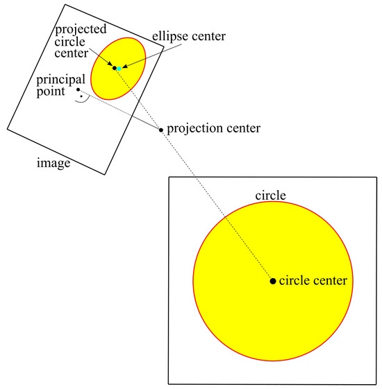
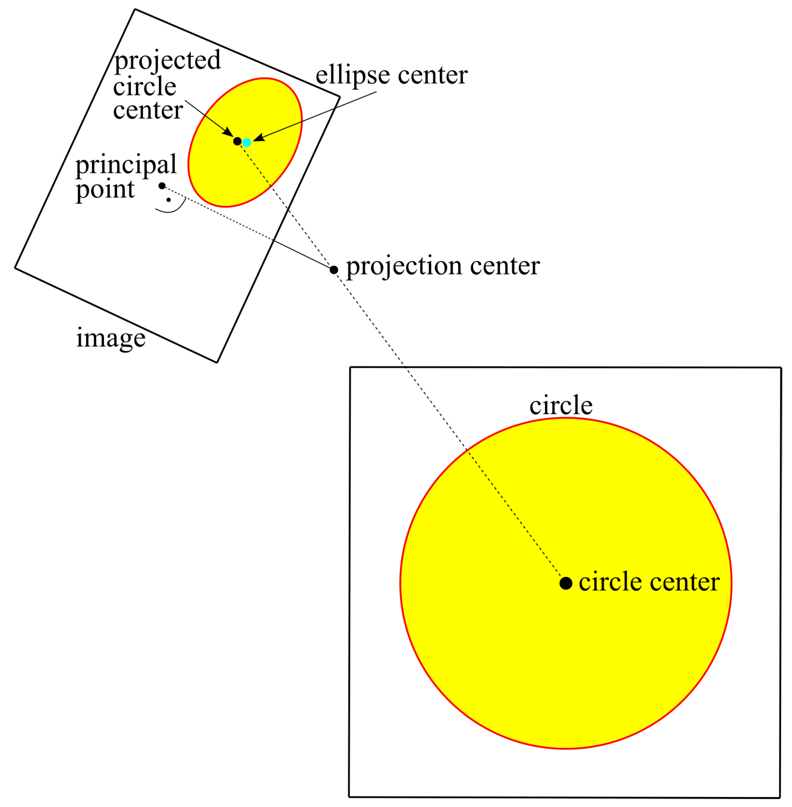
Figure 1 illustrates the circle projection onto an image from an oblique view, where the discrepancy between the ellipse center and the projected circle center is depicted.

One possible method for avoiding eccentricity errors was developed by Andresen and Helsch [4]. They introduced the image ellipse contour points as observations in their bundle adjustment instead of the ellipse centers and, thus, did not have conflicts with discrepancies to the projected circle centers.

When using the standard pinhole model, the error can be minimized by the usage of small target sizes, nearly perpendicular viewing directions and large target-to-camera distances. However, these measures may be in conflict with requirements of photogrammetric network design principles aiming at maximizing accuracy. Dold [5] proposed a simple expression for the eccentricity using a 2D scheme. He also computed a simulation to analyze the influence on the parameter estimation in a bundle adjustment. He observed a slight influence on the residuals and the object coordinates, but a higher influence on the interior and exterior orientation parameters. Heikkilä and Silvén [6] presented a four-step calibration procedure, including a direct linear transformation and a compensation of the eccentricity of circular features. A 3D extension to Dold’s expression was given by Ahn et al. [7]. They also discussed the eccentricity correction with known radii and normals of the circles. Otepka and Fraser [8] proposed an extended bundle adjustment, which took the eccentricity into account, in which the implicit parameters of the image ellipses were used as observations, and in which circle radii as well as normals were introduced as unknowns. Wrobel [9] also considered the perspective projections of circular targets and discussed three different approaches for their mathematical description. He also pointed out that there are two pairs of circle center and normal which lead to the same image ellipse. Another approximation of the eccentricity correction can be obtained by the use of targets with concentric circles shown by He et al. [10] based on the idea of Kim et al. [11]. He et al. [10] showed that the remaining approximation error is negligible. Luhmann [12] computed the projections of simulated circle contour points and performed an ellipse fit with the projected points to get the ellipse center as well as the eccentricity. Matsuoka and Maruyama [13] proposed a complex calculation rule to compute the ellipse parameters from a given circle center, radius and normal, as well as interior and exterior orientation. Yang and Fang [14], Shen et al. [15] also discussed the eccentricity in combination with lens distortion effects and Shen et al. [15] proposed an iterative refinement method. The image matching of circular targets can also cause eccentricity when using affine patch transformation models. However, advanced models, such as the projective transformation as proposed by Bethmann and Luhmann [16], can avoid this issue.

The article at hand is an extended and improved version of [1]. It describes the eccentricity mathematically and provides an extension to the collinearity equations for circles that can be used easily, which is shown in Section 3. Then, in Section 4, five possible correction methods are discussed:

• Section 4.1 presents a correction applied to the image coordinates that is based on the eccentricity computation in the previous section.
• Section 4.2 reviews the dual ring correction in the image space of He et al. [10].
• In Section 4.3, the pinhole model for circles is used as the core for the bundle adjustment.
• In Section 4.4, we present our new extended bundle adjustment.
• Section 4.5 describes and discusses the alternative model by Andresen and Helsch [4] that uses the image ellipse contour points as observations.

After this, the methods are validated in Section 5. In the fourth and fifth correction procedure, the radii of the circles are a part of the model that can either be introduced as unknowns or as constants in a bundle adjustment. This means that they also can be used for the definition of the scale, as outlined in Section 6. Thsi article ends with a conclusion. In Appendix A, the estimation of the circle normals for concentric circle targets is discussed.

3. Mathematical Description of the Eccentricity

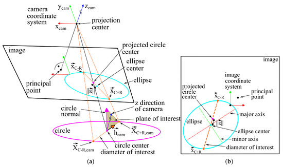
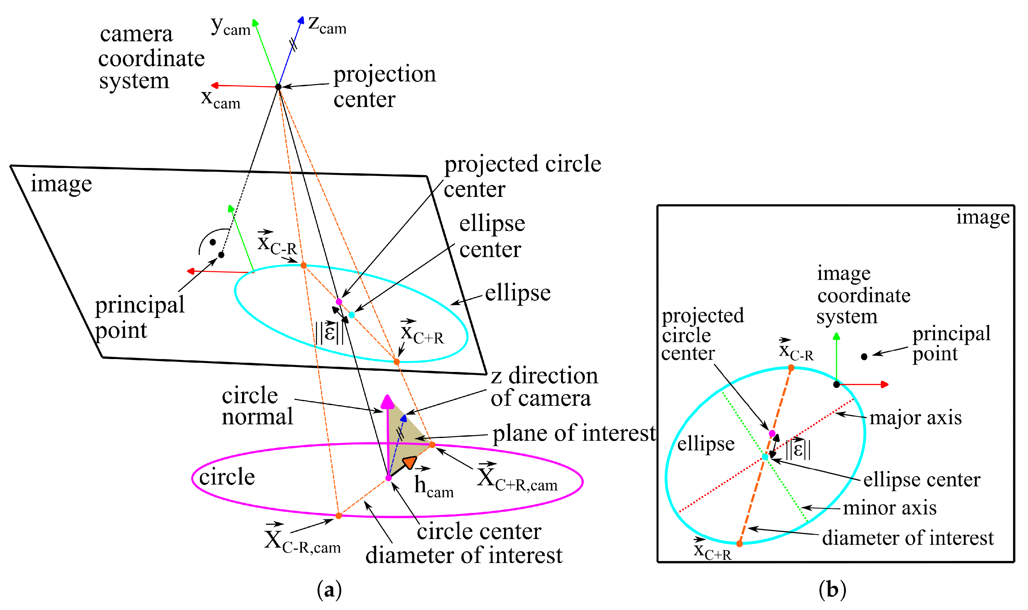
Dold [5] shows a calculation for a 2D scheme in his Equation (2) that works with opposite circle points on a diameter. In order to apply his method in 3D (similar to [7]), the correct circle diameter has to be chosen. This diameter lies in the plane that includes the circle center ${\overrightarrow{X}}_C$, the normal vector ${\overrightarrow{n}}_C$ and the optical axis (z direction of the camera frame). This is the only diameter whose projection contains the ellipse center and the projected circle center. We compute the corresponding direction vector by intersecting this plane with the circle plane. First, the circle center and the circle normal (with $\left|\right|{\overrightarrow{n}}_C\left|\right|=1$) are transformed into the camera frame (Equation (1)). The z direction of the camera frame is ${\left(\begin{array}{ccc}\hfill 0& 0& 1\hfill \end{array}\right)}^T$.

$$\begin{array}{ccc}{\overrightarrow{n}}_{C,cam}& =& \hfill {\mathbf{R}}^T·{\overrightarrow{n}}_C\hfill \\ {\overrightarrow{X}}_{C,cam}& =& {\mathbf{R}}^T·({\overrightarrow{X}}_C-{\overrightarrow{X}}_{projC})\end{array}$$

(1)

where

• $\mathbf{R}$ = rotation matrix of the camera;
• ${\overrightarrow{X}}_{projC}$ = projection center of the camera;
• ${\overrightarrow{X}}_{C,cam}$ = circle center in camera frame;
• ${\overrightarrow{n}}_{C,cam}$ = circle normal in camera frame.

The illustration in Figure 2 shows the projection of a circle (in magenta) into an image where it appears as an ellipse (cyan). The diameter of interest is also depicted in orange. The direction vector ${\overrightarrow{h}}_{cam}$ of the diameter in the camera frame is computed by applying the cross-product two times, which is valid for ${\overrightarrow{n}}_{C,cam}\ne {\left(\begin{array}{ccc}\hfill 0& 0& 1\hfill \end{array}\right)}^T$:

$${\overrightarrow{h}}_{cam}={\overrightarrow{n}}_{C,cam}\times {\displaystyle \frac{{\overrightarrow{n}}_{C,cam}\times \left(\begin{array}{c}\hfill 0\\ \hfill 0\\ \hfill 1\end{array}\right)}{\left|\right|{\overrightarrow{n}}_{C,cam}\times \left(\begin{array}{c}\hfill 0\\ \hfill 0\\ \hfill 1\end{array}\right)\left|\right|}}={\displaystyle \frac{\left(\begin{array}{c}{n}_{C,cam,x}·n_{C,cam,z}\\ n_{C,cam,y}·n_{C,cam,z}\\ -n_{C,cam,x}^2-n_{C,cam,y}^2\end{array}\right)}{\sqrt{n_{C,cam,x}^2+n_{C,cam,y}^2}}}$$

(2)

Thus, the two opposite circle points on this diameter are

$${\overrightarrow{X}}_{C\pm R,cam}={\overrightarrow{X}}_{C,cam}\pm R_C·{\overrightarrow{h}}_{cam}$$

(3)

where $R_C$ = radius of circle.

After this, the circle points ${\overrightarrow{X}}_{C+R,cam}$ and ${\overrightarrow{X}}_{C-R,cam}$ are projected onto the image:

$${\overrightarrow{x}}_{C\pm R}={\overrightarrow{x}}_p-{\displaystyle \frac{c}{Z_{C\pm R,cam}}}·\left(\begin{array}{c}{X}_{C\pm R,cam}\\ Y_{C\pm R,cam}\end{array}\right)$$

(4)

where

• ${\overrightarrow{x}}_p$ = principal point vector;
• c = principal distance.

The ellipse center ${\overrightarrow{x}}_{ell,c}$ is then obtained by averaging the projected circle points at the ends of the diameter:

$${\overrightarrow{x}}_{ell,c}={\displaystyle \frac{1}{2}}·({\overrightarrow{x}}_{C+R}+{\overrightarrow{x}}_{C-R})$$

(5)

Inserting and simplifying yields

$$\begin{array}{c}\hfill x_{ell,c}=x_p-c·{\displaystyle \frac{X_{C,cam}·Z_{C,cam}+R_C^2·n_{C,cam,x}·n_{C,cam,z}}{Z_{C,cam}^2-R_C^2·(n_{C,cam,x}^2+n_{C,cam,y}^2)}}\\ \hfill y_{ell,c}=y_p-c·{\displaystyle \frac{Y_{C,cam}·Z_{C,cam}+R_C^2·n_{C,cam,y}·n_{C,cam,z}}{Z_{C,cam}^2-R_C^2·(n_{C,cam,x}^2+n_{C,cam,y}^2)}}\end{array}$$

(6)

where ${\left(\begin{array}{c}{x}_{ell,c},y_{ell,c}\end{array}\right)}^T$ = ellipse center in image coordinate system.

Equation (6) is simple to use and shows how to compute the ellipse center coordinates with a given exterior image orientation, interior orientation, and circle center, radius, and normal. These equations can also be considered as extended collinearity equations for circles.

If $R_c=0$ (circle = point) or if ${\overrightarrow{n}}_{C,cam}={\left(\begin{array}{ccc}\hfill 0& 0& 1\hfill \end{array}\right)}^T$ (perpendicular view), Equation (6) will lead to the collinearity equations for points (standard pinhole model), resulting in the projected circle center coordinates ${\begin{array}{c}\hfill x_{C,c},y_{C,c}\end{array}}^T$

$$\begin{array}{c}{x}_{C,c}=x_p-c·{\displaystyle \frac{X_{C,cam}}{Z_{C,cam}}}\hfill \\ y_{C,c}=y_p-c·{\displaystyle \frac{Y_{C,cam}}{Z_{C,cam}}}\hfill \end{array}$$

(7)

Equation (6) can also be extended by lens distortion correction. In the paper at hand, the model of Brown [17] and El-Hakim [18] is used; it is shown in Algorithm 1.

Algorithm 1 Lens distortion correction $distortionCorrection$

Input:  $x_{cam}, y_{cam}, A_1, A_2, A_3, B_1, B_2, C_1, C_2$ Radial-symmetric lens distortion correction: $\left(\begin{array}{c}{\Delta x}_{rad}\\ {\Delta y}_{rad}\end{array}\right)=(A_1·r^2+A_2·r^4+A_3·r^6)·\left(\begin{array}{c}{x}_{cam}\\ y_{cam}\end{array}\right)$ with $r=\sqrt{x_{cam}^2+y_{cam}^2}$ Decentering lens distortion correction: $\left(\begin{array}{c}{\Delta x}_{dec}\\ {\Delta y}_{dec}\end{array}\right)=\left(\begin{array}{c}{B}_1·(r^2+2·x_{cam}^2)+2·B_2·x_{cam}·y_{cam}\\ B_2·(r^2+2·y_{cam}^2)+2·B_1·x_{cam}·y_{cam}\end{array}\right)$ Correction for affinity and non-orthogonality: $\left(\begin{array}{c}{\Delta x}_{aff}\\ {\Delta y}_{aff}\end{array}\right)=\left(\begin{array}{c}{C}_1·x_{cam}+C_2·y_{cam}\\ 0\end{array}\right)$ Full lens distortion correction: $\left(\begin{array}{c}\Delta x_{dist}\\ \Delta y_{dist}\end{array}\right)=\left(\begin{array}{c}{\Delta x}_{rad}\\ {\Delta y}_{rad}\end{array}\right)+\left(\begin{array}{c}{\Delta x}_{dec}\\ {\Delta y}_{dec}\end{array}\right)+\left(\begin{array}{c}{\Delta x}_{aff}\\ {\Delta y}_{aff}\end{array}\right)$ where     xcam, ycam = image point in camera frame A1, A2, A3 = radial-symmetric lens distortion parameters B1, B2 = decentering lens distortion parameters C1, C2 = parameters for affinity, shear Output:  Lens distortion correction ${\Delta x}_{dist},{\Delta y}_{dist}$

Algorithm 2 shows the pinhole model for circles including lens distortion correction.

Algorithm 2 Extended pinhole model for circles (ellipse center of circle projection) with lens distortion correction

Input:  ${\overrightarrow{X}}_{projC}, \mathbf{R}, {\overrightarrow{X}}_C, {\overrightarrow{n}}_C, R_C, c, x_p, y_p, A_1, A_2, A_3, B_1, B_2, C_1, C_2$ Transform the circle center and normal into camera frame: ${\overrightarrow{X}}_{C,cam}={\mathbf{R}}^T·({\overrightarrow{X}}_C-{\overrightarrow{X}}_{projC})$ ${\overrightarrow{n}}_{cam}={\mathbf{R}}^T·{\overrightarrow{n}}_C$ Ellipse center coordinates of the circle projection in camera frame (Equation (26)): $x_{ell,c,cam}=-c·{\displaystyle \frac{X_{C,cam}·Z_{C,cam}+R_C^2·n_{C,cam,x}·n_{C,cam,z}}{Z_{C,cam}^2-R_C^2·(n_{C,cam,x}^2+n_{C,cam,y}^2)}}$ $y_{ell,c,cam}=-c·{\displaystyle \frac{Y_{C,cam}·Z_{C,cam}+R_C^2·n_{C,cam,y}·n_{C,cam,z}}{Z_{C,cam}^2-R_C^2·(n_{C,cam,x}^2+n_{C,cam,y}^2)}}$ Lens distortion correction and principal point shift applied to ellipse center: $\Delta {\overrightarrow{x}}_{ell,c,dist}=distortionCorrection\left({\overrightarrow{x}}_{ell,c,cam}\right)$ ${\overrightarrow{x}}_{ell,c,dist}={\overrightarrow{x}}_p+{\overrightarrow{x}}_{ell,c,cam}+\Delta {\overrightarrow{x}}_{ell,c,dist}$ Output:  Lens distortion corrected ellipse center in image system: $x_{ell,c,dist},y_{ell,c,dist}$

3.1. Eccentricity Calculation

The eccentricity error $\overrightarrow{ϵ}$ is computed by the difference of the ellipse center and the projected circle center:

$$\overrightarrow{ϵ}={\overrightarrow{x}}_{C,c}-{\overrightarrow{x}}_{ell,c}$$

(8)

Inserting this into Equation (6) as well as Equation (7) and simplifying yields

$$\begin{array}{cc}\hfill {ϵ}_x& ={\displaystyle \frac{c·R_C^2}{Z_{C,cam}}}·{\displaystyle \frac{Z_{C,cam}·n_{C,cam,x}·n_{C,cam,z}+X_{C,cam}·(n_{C,cam,x}^2+n_{C,cam,y}^2)}{Z_{C,cam}^2-R_C^2·(n_{C,cam,x}^2+n_{C,cam,y}^2)}}\hfill \\ \hfill {ϵ}_y& ={\displaystyle \frac{c·R_C^2}{Z_{C,cam}}}·{\displaystyle \frac{Z_{C,cam}·n_{C,cam,y}·n_{C,cam,z}+Y_{C,cam}·(n_{C,cam,x}^2+n_{C,cam,y}^2)}{Z_{C,cam}^2-R_C^2·(n_{C,cam,x}^2+n_{C,cam,y}^2)}}\hfill \end{array}$$

(9)

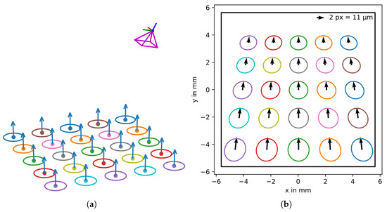
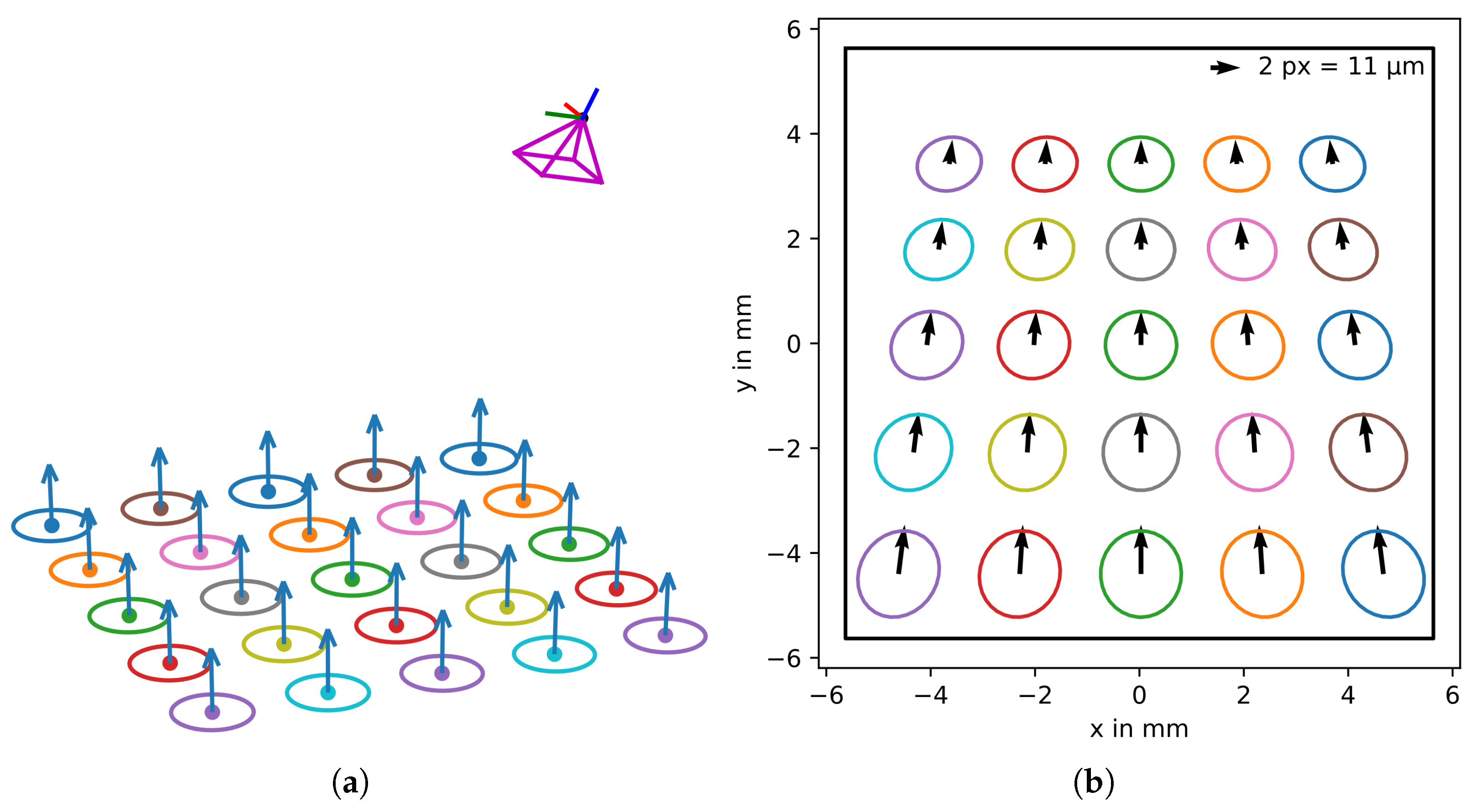
Equation (8) (or Equation (9)) can now be used to calculate the eccentricity for different scenarios. An example is demonstrated in Figure 3, where a planar grid of 5 × 5 circles with 20 mm radius is defined with a grid size of 60 mm. The assumed projection center of the camera (2048 × 2048 px, pixel size: 5.5 µm, focal length: 12 mm) has a horizontal distance of 120 mm and vertical distance of 330 mm to the centroid. The optical axis points to the centroid and has an angle of ≈20° to the plane’s normal. The computed ellipses are plotted and the eccentricities are shown as a vector field. In this case, the deviations reach values of up to 3.3 px, which is about two orders of magnitude larger than the precision potential of ellipse operators [19].

The length of the eccentricity vector is computed with the components of Equation (9):

$$\begin{array}{cc}\left|\right|\overrightarrow{ϵ}\left|\right|=\hfill & {\displaystyle \frac{c·R_C^2·\left|\right|n_{C,cam,z}\left|\right|}{Z_{C,cam}^2}}·{\displaystyle \frac{1}{1-\frac{R_C^2}{Z_{C,cam}^2}·(n_{C,cam,x}^2+n_{C,cam,y}^2)}}·\hfill \\ & \hfill \sqrt{{(n_{C,cam,x}+\frac{X_{C,cam}·(n_{C,cam,x}^2+n_{C,cam,y}^2)}{Z_{C,cam}·n_{C,cam,z}})}^2+{(n_{C,cam,y}+\frac{Y_{C,cam}·(n_{C,cam,x}^2+n_{C,cam,y}^2)}{Z_{C,cam}·n_{C,cam,z}})}^2}\end{array}$$

(10)

3.2. Eccentricity Approximation

In addition to the calculation of eccentricity in Section 3.1, this section shows an approximation of the eccentricity as is applied in a later section. The denominator in Equation (6) can be transformed with the assumption $Z_{C,cam}^2\gg R_C^2$:

$$Z_{C,cam}^2-R_C^2·(n_{C,cam,x}^2+n_{C,cam,y}^2)\approx Z_{C,cam}^2$$

(11)

Equation (6) becomes simplified as follows where the fraction is split:

$$\begin{array}{c}\hfill x_{ell,c}\approx \underset{=x_{C,c}}{\underbrace{x_p-c·{\displaystyle \frac{X_{C,cam}}{Z_{C,cam}}}}}-\underset{=e_x\approx {ϵ}_x}{\underbrace{{\displaystyle \frac{c·R_C^2·n_{C,cam,x}·n_{C,cam,z}}{Z_{C,cam}^2}}}}\\ \hfill y_{ell,c}\approx \underset{=y_{C,c}}{\underbrace{y_p-c·{\displaystyle \frac{Y_{C,cam}}{Z_{C,cam}}}}}-\underset{=e_y\approx {ϵ}_y}{\underbrace{{\displaystyle \frac{c·R_C^2·n_{C,cam,y}·n_{C,cam,z}}{Z_{C,cam}^2}}}}\end{array}$$

(12)

The left parts of the right-hand side are the coordinates of the projected circle center ${\overrightarrow{x}}_{c,c}$, and the right parts are summarized in $e_x\approx {ϵ}_x$ and $e_y\approx {ϵ}_y$, representing an approximation for the eccentricity.

$$\overrightarrow{ϵ}\approx \overrightarrow{e}={\displaystyle \frac{c·R_C^2·n_{C,cam,z}}{Z_{C,cam}^2}}·\left(\begin{array}{c}{n}_{C,cam,x}\\ n_{C,cam,y}\end{array}\right)$$

(13)

The approximation in Equation (13) shows the dependencies of the eccentricity $e\approx ϵ$:

• e is proportional to the principal distance: $e\sim c$.
• e is proportional to the squared radius: $e\sim R_C^2$.
• e is inversely proportional to the squared z coordinate in the camera frame: $e\sim Z_{C,cam}^{-2}$.
• e can be eliminated for a perpendicular view with $n_{C,cam,x}=n_{C,cam,y}=0$ or $R_C=0$.

The length of the approximate vector is

$$\left|\right|\overrightarrow{e}\left|\right|={\displaystyle \frac{c·R_C^2·\left|\right|n_{C,cam,z}\left|\right|}{Z_{C,cam}^2}}·\sqrt{n_{C,cam,x}^2+n_{C,cam,y}^2}$$

(14)

with the upper bound (because $n_{C,cam,x}^2+n_{C,cam,y}^2\le 1$ and $\left|\right|n_{C,cam,z}\left|\right|\le 1$)

$$\left|\right|\overrightarrow{e}\left|\right|\le {\displaystyle \frac{c·R_C^2}{Z_{C,cam}^2}}$$

(15)

The remaining error in the vector length can be computed by the difference between Equations (10) and (15):

$$\Delta \left|\right|\overrightarrow{e}\left|\right|=\left|\right|\overrightarrow{ϵ}\left|\right|-\left|\right|\overrightarrow{e}\left|\right|$$

(16)

4. Eccentricity Correction Methods

This section shows five different correction methods for the eccentricity. The first two are applied in the image space, where an offset is added to the observed ellipse center coordinates to eliminate the systematic error when using the standard pinhole model. The next two correction methods work through a model adaptation, wherein the pinhole model is modified so that the output of the mapping process is the ellipse center rather than the projected circle center. The last method works with an implicit condition for the observed image ellipse contour points.

4.1. Image Coordinate Correction with Known Radius and Normal

The correction in this section is applied in the image space using Equation (8) (or the approximation in Equation (13)), where the normal directions and the radii of the circular targets are assumed to be known. In the case of a spatial resection (SR) or a bundle adjustment (BA), the interior and exterior orientation parameters (EOP) can be obtained without eccentricity correction in a first iteration with the standard pinhole model and without eccentricity correction. After this, the corrections are computed with the results of step one. The corrections can also be updated in further iterations. Algorithm 3 summarizes the procedure. This method is suitable for special cases such as planar target fields, where the normals can be obtained by a plane fit. Another possibility is the use of a test field with target groups of at least three coplanar targets so that the normals can be calculated as triangle normals, as was also proposed by Ahn et al. [7].

Algorithm 3 Space resection or bundle adjustment with eccentricity correction in image space with known radius and normal

Input:  $R_C$ Obtain EOP in SR or BA with standard pinhole model without ecc. corr. Compute/obtain circle normals ${\overrightarrow{n}}_C$.  Do    3.1. Compute $\overrightarrow{ϵ}$ using Equation (8) (or Equation (13)) with c, ${\overrightarrow{n}}_C$, $R_C$ and (updated) EOP.    3.2. Apply ecc. corr. to image ellipse centers: ${\overrightarrow{x}}_{C,c}={\overrightarrow{x}}_{ell,c}+\overrightarrow{ϵ}$.    3.3. Compute SR or BA with standard pinhole model and the corrected image points ${\overrightarrow{x}}_{C,c}$ and update c as well as EOP.    (3.4. Update ${\overrightarrow{n}}_C$ in case of BA)  While $\left|\right|{\overrightarrow{ϵ}}_j-{\overrightarrow{ϵ}}_{j-1}\left|\right|>\delta$ where       j $=\mathrm{index} \mathrm{of} \mathrm{iteration}$      δ $=\mathrm{convergence} \mathrm{threshold}$ Output:  Eccentricity $\overrightarrow{ϵ}$ and SR or BA outputs

Note that the eccentricity calculation in this method is robust against random errors of the ellipse measurement, as is computed with the IOP, EOP, and circle parameters.

4.2. Correction with Concentric Circle Targets

He et al. [10] proposed a procedure where the eccentricity can be corrected approximately with the help of the measurement of the ellipse centers of two concentric circles and the knowledge of their radii. The correction can be derived using the approximation shown in Section 3.2. For concentric circles, Equation (13) only differs in the radii $R_{c,1}$ and $R_{c,2}$, and the following ratio can be derived:

$${\displaystyle \frac{e_{x,1}}{e_{x,2}}}={\displaystyle \frac{e_{y,1}}{e_{y,2}}}={\displaystyle \frac{R_{C,1}^2}{R_{C,2}^2}}$$

(17)

This ratio is equivalent to

$${\overrightarrow{e}}_2={\displaystyle \frac{R_{C,2}^2}{R_{C,1}^2}}·{\overrightarrow{e}}_1$$

(18)

Furthermore, the system from Equation (12) is used:

$$\begin{array}{cc}\hfill {\overrightarrow{x}}_{ell,c,1}& \approx {\overrightarrow{x}}_{C,c}-{\overrightarrow{e}}_1\hfill \\ \hfill {\overrightarrow{x}}_{ell,c,2}& \approx {\overrightarrow{x}}_{C,c}-{\overrightarrow{e}}_2\hfill \end{array}$$

(19)

Equation (18) is inserted into the second equation in Equation (19):

$$\begin{array}{cc}\hfill {\overrightarrow{x}}_{ell,c,1}& \approx {\overrightarrow{x}}_{C,c}-{\overrightarrow{e}}_1\hfill \\ \hfill {\overrightarrow{x}}_{ell,c,2}& \approx {\overrightarrow{x}}_{C,c}-{\displaystyle \frac{R_{C,2}^2}{R_{C,1}^2}}·{\overrightarrow{e}}_1\hfill \end{array}$$

(20)

Subtracting the first from the second equation in Equation (18) and rearranging yields the approximation for the eccentricity of the first ellipse center:

$${\overrightarrow{ϵ}}_1\approx {\overrightarrow{e}}_1={\displaystyle \frac{{\overrightarrow{x}}_{ell,c,2}-{\overrightarrow{x}}_{ell,c,1}}{1-{\left(\frac{R_{C,2}}{R_{C,1}}\right)}^2}}$$

(21)

Then, the projected circle center can be estimated by inserting Equation (21) into the first equation in Equation (19). Note that the correction can be computed without the knowledge of the circle normal.

$${\overrightarrow{x}}_{C,c}\approx {\overrightarrow{x}}_{ell,c,1}+{\displaystyle \frac{{\overrightarrow{x}}_{ell,c,2}-{\overrightarrow{x}}_{ell,c,1}}{1-{\left(\frac{R_{C,2}}{R_{C,1}}\right)}^2}}$$

(22)

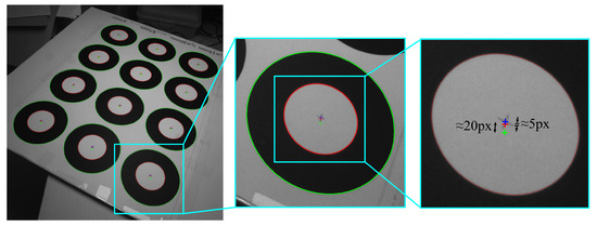
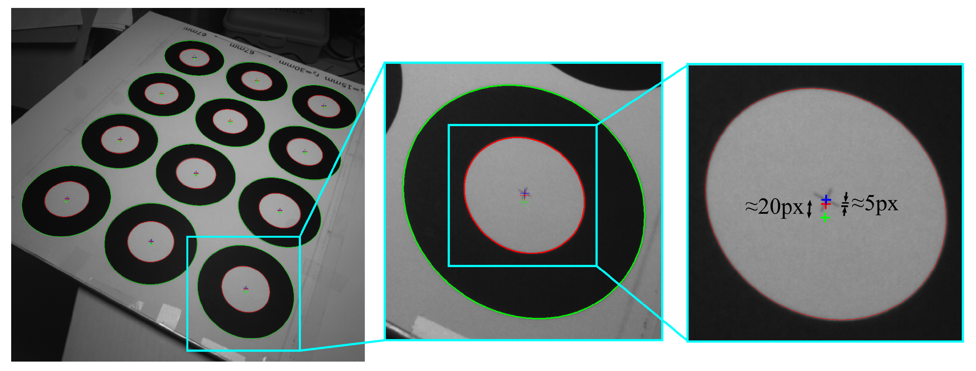
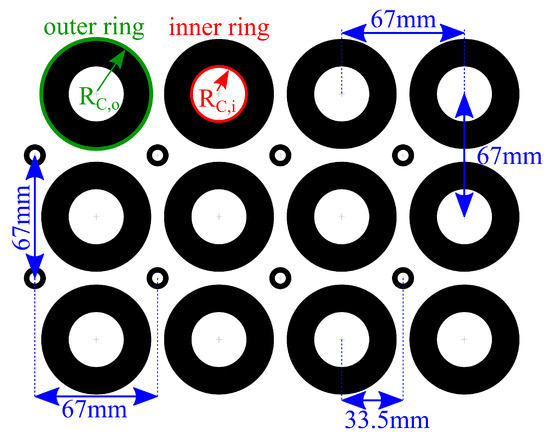
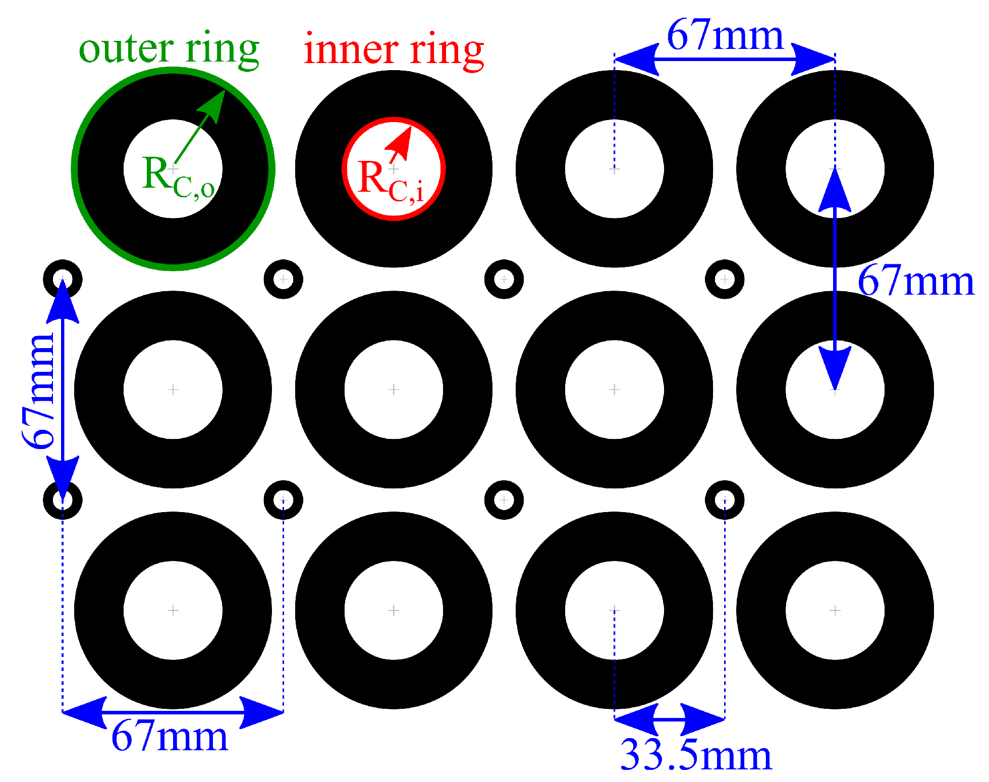
Figure 4 shows an example with two ellipse measurements (red and green) and the corrected point (blue cross) that represents the projected circle center of the concentric circles. In the center of the circular target, a black cross was printed that can also be seen. The lengths of the minor and major axes of the target’s inner ring (with a diameter of 30 mm) were 291 and 255 px. For the outer ring with 60 mm diameter, the axes’ lengths were 585 and 514 px.

Algorithm 4 summarizes the procedure for a bundle adjustment or space resection, including the eccentricity correction with the concentric circle targets.

Note that, for the image measurement of the two rings, a suitable resolution of the concentric circle targets is required, especially for strongly oblique views. The thickness of the circle ring should have several pixels in the image for the usage of edge detectors as the star [20] or the Zhou operator [21]. Inner circles of the targets with too small semi-minor axes should be ignored to avoid conflicts due to this issue. Also note that the eccentricity computation can be influenced by the random errors of the both ellipse measurements, especially for small targets. Besides, Appendix A shows three approaches to obtain the normals of concentric circle targets.

Algorithm 4 Space resection or bundle adjustment with eccentricity correction in image space using concentric circle targets.

Input:  Target radius ratio $R_{C,2}/R_{C,1}$, ellipse center coordinates: ${\overrightarrow{x}}_{ell,c,1}$, ${\overrightarrow{x}}_{ell,c,2}$ Compute circle center using the two measured ellipse centers: ${\overrightarrow{x}}_{C,c}\approx {\overrightarrow{x}}_{ell,c,1}+{\displaystyle \frac{{\overrightarrow{x}}_{ell,c,2}-{\overrightarrow{x}}_{ell,c,1}}{1-{\left(\frac{R_{C,2}}{R_{C,1}}\right)}^2}}$ Compute SR or BA with standard pinhole model and the corrected image points ${\overrightarrow{x}}_{C,c}$ Output:  SR outputs or BA outputs

4.3. Model-Side Eccentricity Correction with Given Normal and Radius

In contrast to last two subsections where eccentricity corrections are applied in the image space, this subsection focuses on an adaptation of the pinhole model to avoid eccentricity errors. For this correction method on the model side, the standard pinhole model is replaced by the adapted pinhole model for circles (Equations (1) and (6), Algorithm 2) so that the ellipse center coordinates from the circle projection are calculated directly in the adapted model. For the application of the adapted pinhole model for circles, the normals and the radii of the circles must be known. Thus, circle radius and normal are considered as constants here. Like in Section 4.1, this procedure can only be applied to a BA or SR for special cases where the normals are known or can easily be estimated, such as planar test fields or coplanar target groups of at least three targets.

In Equation (23), the ellipse center is represented as a function of the EOP, IOP, and circle center, as well as its radius and normal.

$${\overrightarrow{x}}_{ell,c,dist,comp}=\overrightarrow{f}(\underset{\mathrm{unknowns}}{\underbrace{{\overrightarrow{X}}_{projC}, \mathbf{R}, }}\underset{\mathrm{possible} \mathrm{unknowns}}{\underbrace{{\overrightarrow{X}}_C, c, {\overrightarrow{x}}_p, A_1, A_2, A_3, B_1, B_2, C_1, C_2, }}\underset{\mathrm{constants}}{\underbrace{R_C, {\overrightarrow{n}}_C}})$$

(23)

A BA or SR can be computed by minimizing the sum of squared residuals of the observed ellipse centers from the image measurement and the computed ellipse centers from Equation (23).

$$\sum _i\left|\right|\Delta {\overrightarrow{x}}_{ell,c,dist,i}{\left|\right|}^2\to min$$

(24)

where

• $\Delta {\overrightarrow{x}}_{ell,c,dist,i}$ = ${\overrightarrow{x}}_{ell,c,dist,obs,i}-{\overrightarrow{x}}_{ell,c,dist,comp,i}$;
• i = index of observation (image ellipse).

In case of a BA where the circle centers are possible unknowns, the parameter estimation and eccentricity correction can be performed iteratively. The necessary parameters (EOP, IOP, and circle center coordinates) are estimated using the standard pinhole model in a first iteration. Then, the normals can be computed with the estimated circle centers, and the adapted pinhole model can be applied.

Algorithm 5 shows a strategy for a bundle adjustment with the model adaption.

Note that the eccentricity calculation of this method is also robust against random errors of the ellipse measurement, as it is computed with the EOP, IOP and circle parameters.

Algorithm 5 Bundle adjustment with the model adaption for circles.

Input:  Target radii $R_C$, measured ellipse center coordinates ${\overrightarrow{x}}_{ell,c}$ Compute BA with standard pinhole model (IOP, EOP, circle centers) Do  Compute circle normals with plane fit for coplanar target groups Compute BA with adapted pinhole model for circles (IOP, EOP, circle centers) While  any($\left|\right|{dx}_j\left|\right|>{\delta }_j$ for $j\in \{1,\dots ,u\}$) where     dxj$=\mathrm{correction}\mathrm{for}$ jth $\mathrm{parameter}$     δj $=\mathrm{convergence}\mathrm{threshold}\mathrm{for}$ jth $\mathrm{parameter}$     u $=\mathrm{number}\mathrm{of}\mathrm{parameters}$ Output:  Estimated BA outputs: IOP, EOP, circle centers

4.4. Extended Bundle Adjustment

The fourth approach to avoid eccentricity errors adapts the idea of an extended bundle adjustment by Otepka and Fraser [8]. They used the implicit ellipse parameters derived from the image measurements as observations to obtain the circle center coordinates, the normal and the radius as unknowns in a BA. In the article at hand, we propose a new different approach to the extended bundle adjustment, where, in addition to the ellipse center coordinates, the lengths of the ellipse semi-axes are used as observations and the lens distortion correction is also considered. Compared to the method by Otepka and Fraser [8], the implicit parameters are not used as observations in our bundle adjustment. However, we also computed implicit parameters, but only as an intermediary result in our pinhole model. In contrast to Section 4.3, this algorithm is not limited to special cases because the circle normals as well as the circle radii belong to the unknowns that are estimated in the BA, so that only initial values have to be obtained.

In order to compute the ellipse center and semi-axes in the pinhole model, the coefficients of the implicit ellipse form are calculated with the method of Matsuoka and Maruyama [13] that fulfill the following equation for the image ellipse contour points $(x_Q,y_Q)$ (see Equations (25)–(28) partially adapted from [13]).

$$p_{xx}·x_Q^2+p_{yy}·y_Q^2+p_{cc}·c^2+2·p_{xy}·x_Q·y_Q+2·p_{xc}·x_Q·c+2·p_{yc}·y_Q·c=0$$

(25)

The coefficients are computed using the circle normal and the circle center in the camera frame after applying Equation (1):

$$\begin{array}{cc}\hfill p_{xx}=& (n_{C,cam,x}^2+n_{C,cam,y}^2)·Y_{C,cam}^2+2·n_{C,cam,y}·n_{C,cam,z}·Y_{C,cam}·Z_{C,cam}\hfill \\ \hfill & +(n_{C,cam,x}^2+n_{C,cam,z}^2)·Z_{C,cam}^2-n_{C,cam,x}^2·R_C^2\hfill \\ \hfill p_{yy}=& (n_{C,cam,x}^2+n_{C,cam,y}^2)·X_{C,cam}^2+2·n_{C,cam,x}·n_{C,cam,z}·X_{C,cam}·Z_{C,cam}\hfill \\ \hfill & +(n_{C,cam,y}^2+n_{C,cam,z}^2)·Z_{C,cam}^2-n_{C,cam,y}^2·R_C^2\hfill \\ \hfill p_{cc}=& (n_{C,cam,x}^2+n_{C,cam,z}^2)·X_{C,cam}^2+2·n_{C,cam,x}·n_{C,cam,y}·X_{C,cam}·Y_{C,cam}\hfill \\ \hfill & +(n_{C,cam,y}^2+n_{C,cam,z}^2)·Y_{C,cam}^2-n_{C,cam,z}^2·R_C^2\hfill \\ \hfill p_{xy}=& n_{C,cam,x}·n_{C,cam,y}·(Z_{C,cam}^2-R_C^2)-n_{C,cam,x}·n_{C,cam,z}·Y_{C,cam}·Z_{C,cam}\hfill \\ \hfill & -n_{C,cam,y}·n_{C,cam,z}·X_{C,cam}·Z_{C,cam}-(n_{C,cam,x}^2+n_{C,cam,y}^2)·X_{C,cam}·Y_{C,cam}\hfill \\ \hfill p_{xc}=& n_{C,cam,x}·n_{C,cam,z}·(R_C^2-Y_{C,cam}^2)+n_{C,cam,x}·n_{C,cam,y}·Y_{C,cam}·Z_{C,cam}\hfill \\ \hfill & +n_{C,cam,y}·n_{C,cam,z}·X_{C,cam}·Y_{C,cam}+(n_{C,cam,x}^2+n_{C,cam,z}^2)·X_{C,cam}·Z_{C,cam}\hfill \\ \hfill p_{yc}=& n_{C,cam,y}·n_{C,cam,z}·(R_C^2-X_{C,cam}^2)+n_{C,cam,x}·n_{C,cam,y}·X_{C,cam}·Z_{C,cam}\hfill \\ \hfill & +n_{C,cam,x}·n_{C,cam,z}·X_{C,cam}·Y_{C,cam}+(n_{C,cam,y}^2+n_{C,cam,z}^2)·Y_{C,cam}·Z_{C,cam}\hfill \end{array}$$

(26)

The implicit ellipse parameters are then transformed to the parametric form. The ellipse center coordinates are expressed in Equation (27). Note that inserting Equation (26) into Equation (27) and simplifying leads to Equation (6).

$$\begin{array}{c}\hfill x_{ell,c}=x_p-c·{\displaystyle \frac{p_{yy}·p_{xc}-p_{xy}·p_{yc}}{p_{xx}·p_{yy}-p_{xy}^2}}\\ \hfill y_{ell,c}=y_p-c·{\displaystyle \frac{p_{xx}·p_{yc}-p_{xy}·p_{xc}}{p_{xx}·p_{yy}-p_{xy}^2}}\end{array}$$

(27)

The semi-major as well as the semi-minor axes and the inclination are

$$\begin{array}{c}\hfill \begin{array}{c}w=((x_{ell,c}-x_p)·p_{xc}+(y_{ell,c}-y_p)·p_{yc}+p_{cc}·c)·c\end{array}\\ \hfill \widehat{a}=\sqrt{{\displaystyle \frac{-2·w}{p_{xx}+p_{yy}-\sqrt{{(p_{xx}-p_{yy})}^2+4·p_{xy}^2}}}}\\ \hfill \widehat{b}=\sqrt{{\displaystyle \frac{-2·w}{p_{xx}+p_{yy}+\sqrt{{(p_{xx}-p_{yy})}^2+4·p_{xy}^2}}}}\\ \hfill \phi ={\displaystyle \frac{1}{2}}·arctan2(2·p_{xy},p_{yy}-p_{xx})\end{array}$$

(28)

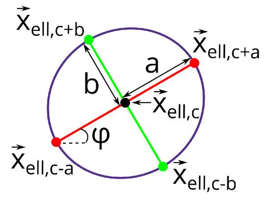
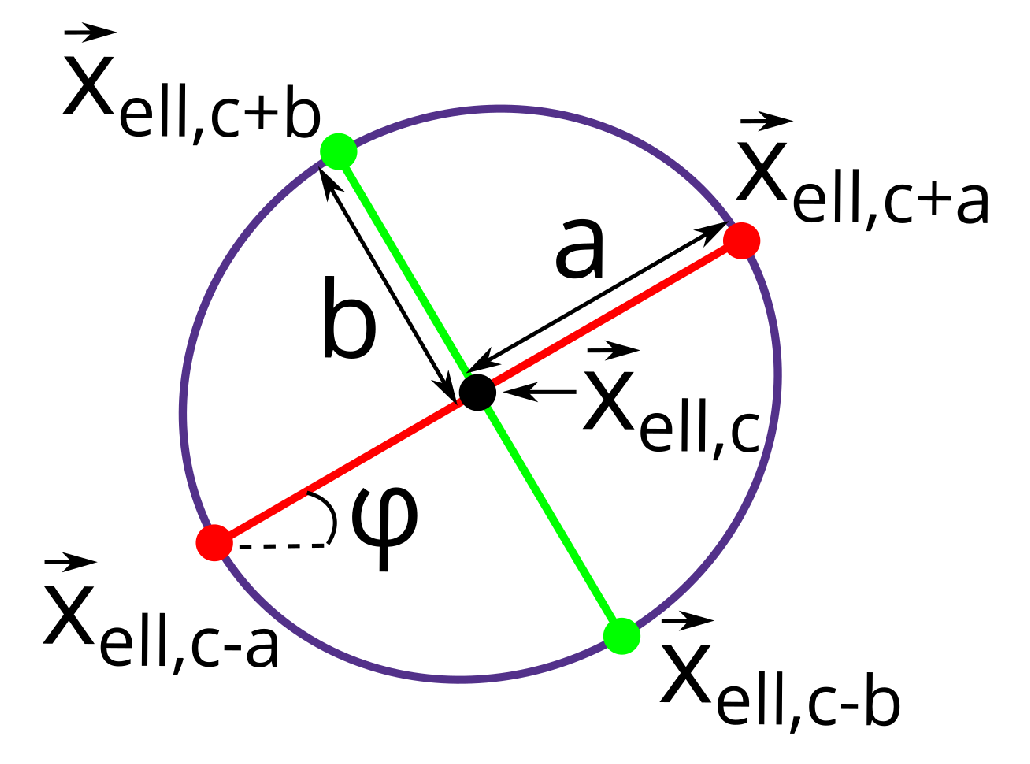
For applying lens distortion correction, first, the four points at main axes (ellipse vertices and ellipse co-vertices, see Figure 5) are computed:

$$\begin{array}{c}\hfill {\overrightarrow{x}}_{ell,c\pm a}={\overrightarrow{x}}_{ell,c}\pm \left(\begin{array}{c}cos\left(\phi \right)\\ sin\left(\phi \right)\end{array}\right)·\widehat{a}\\ \hfill {\overrightarrow{x}}_{ell,c\pm b}={\overrightarrow{x}}_{ell,c}\pm \left(\begin{array}{c}-sin\left(\phi \right)\\ cos\left(\phi \right)\end{array}\right)·\widehat{b}\end{array}$$

(29)

After this, lens distortion correction is computed for the ellipse center ${\overrightarrow{x}}_{ell,c}$ and the ellipse vertices and co-vertices ${\overrightarrow{x}}_{ell,c\pm a}$ and ${\overrightarrow{x}}_{ell,c\pm b}$ with the model in [17,18] represented by the function $distortionCorrection$ (see Algorithm 1):

$$\begin{array}{cc}\hfill \Delta {\overrightarrow{x}}_{ell,c,dist}=& distortionCorrection({\overrightarrow{x}}_{ell,c}-{\overrightarrow{x}}_p)\\ \hfill \Delta {\overrightarrow{x}}_{ell,c\pm a,dist}=& distortionCorrection({\overrightarrow{x}}_{ell,c\pm a}-{\overrightarrow{x}}_p)\\ \hfill \Delta {\overrightarrow{x}}_{ell,c\pm b,dist}=& distortionCorrection({\overrightarrow{x}}_{ell,c\pm b}-{\overrightarrow{x}}_p)\end{array}$$

(30)

The lens distortion corrected semi-axes lengths are then computed as the half distances between the ellipse vertices and co-vertices. For the ellipse center, it is obvious.

$${\overrightarrow{x}}_{ell,c,dist}={\overrightarrow{x}}_{ell,c}+\Delta {\overrightarrow{x}}_{ell,c,dist}$$

(31)

$$a_{dist}={\displaystyle \frac{1}{2}}·\left|\right|{\overrightarrow{x}}_{ell,c+a}+\Delta {\overrightarrow{x}}_{ell,c+a,dist}-{\overrightarrow{x}}_{ell,c-a}-\Delta {\overrightarrow{x}}_{ell,c-a,dist}\left|\right|$$

(32)

$$b_{dist}={\displaystyle \frac{1}{2}}·\left|\right|{\overrightarrow{x}}_{ell,c+b}+\Delta {\overrightarrow{x}}_{ell,c+b,dist}-{\overrightarrow{x}}_{ell,c-b}-\Delta {\overrightarrow{x}}_{ell,c-b,dist}\left|\right|$$

(33)

All in all, the ellipse center and the semi-axes can be computed as a function (Equations (1) and (26)–(33)) of the exterior and interior orientation as well as the circle parameters:

$$\left(\begin{array}{c}{x}_{ell,c,dist,comp}\\ y_{ell,c,dist,comp}\\ a_{dist,comp}\\ b_{dist,comp}\end{array}\right)=\overrightarrow{f}\left({\overrightarrow{X}}_{projC}, \mathbf{R}, {\overrightarrow{X}}_C, R_C, {\overrightarrow{n}}_C, c, {\overrightarrow{x}}_p, A_1, A_2, A_3, B_1, B_2, C_1, C_2\right)$$

(34)

Algorithm 6 summarizes the steps for the computation of the ellipse parameters from the circle projection.

Algorithm 6 Ellipse parameters of circle projection with lens distortion correction

Input:  ${\overrightarrow{X}}_{projC}, \mathbf{R}, {\overrightarrow{X}}_C, R_C, {\overrightarrow{n}}_C, c, {\overrightarrow{x}}_p, A_1, A_2, A_3, B_1, B_2, C_1, C_2$ Transform the circle center and normal into camera frame: ${\overrightarrow{X}}_{C,cam}={\mathbf{R}}^T·({\overrightarrow{X}}_C-{\overrightarrow{X}}_{projC})$ ${\overrightarrow{n}}_{C,cam}={\mathbf{R}}^T·{\overrightarrow{n}}_C$ Compute implicit ellipse parameters of the circle projection using Equation (26) Compute ellipse center, semi-axes and inclination using Equations (27) and (28) Compute ellipse vertices and co-vertices using Equation (29) Compute lens distortion correction for the ellipse center, the ellipse vertices and co-vertices using Equation (30) Apply lens distortion corr. to ellipse center and semi-axes using Equations (31)–(33) Output:  $x_{ell,c,dist}, y_{ell,c,dist}, a_{dist}, b_{dist}$

The measurement of the ellipse center and the semi-axes are considered as observations (${\overrightarrow{x}}_{ell,c,dist,obs}, a_{dist,obs}, b_{dist,obs}$) so that the parameters in the function of Equation (34) can be estimated in a bundle adjustment by minimizing the residuals between the measurements and the computed values of Equation (34) (parametric adjustment [22]):

$$\sum _i\left(\right||\Delta {\overrightarrow{x}}_{ell,c,dist,i}{\left|\right|}^2+\Delta a_{dist,i}^2+\Delta b_{dist,i}^2)\to min$$

(35)

where

• $\Delta {\overrightarrow{x}}_{ell,c,dist,i}$ = ${\overrightarrow{x}}_{ell,c,dist,obs,i}-{\overrightarrow{x}}_{ell,c,dist,comp,i}$;
• $\Delta a_{dist,i}$ = $a_{dist,obs,i}-a_{dist,comp,i}$;
• $\Delta b_{dist,i}$ = $b_{dist,obs,i}-b_{dist,comp,i}$;
• i = index of observation (image ellipse).

The Jacobian matrix can be calculated with numerical derivatives by central differences applied to Equation (34). Note that, for each circle normal, one constraint is introduced (unit vector condition), which increases the computational effort accordingly.

Also note that the eccentricity calculation of this method is also robust against random errors of the ellipse measurement, as it is computed with the EOP, IOP and circle parameters.

4.5. Bundle Adjustment with Contour Points

This section describes the method of Andresen and Helsch [4], where the image ellipse contour points are introduced as observations. The model can be used as a core of the bundle adjustment instead of the collinearity equations. In this procedure, an eccentricity error cannot occur because the ellipse centers do not appear in the model.

The required constraint is derived in the following. First, the ray equation in Equation (36) is considered. The ray starts from the projection center and points to the contour point. The direction vector is defined by the rotated image ellipse contour point, which is lens distortion-corrected using the iterative scheme in Algorithm 7.

$$\begin{array}{cc}\hfill {\overrightarrow{X}}_{ray}\left(k\right)& ={\overrightarrow{X}}_{projC}+k·\mathbf{R}·\left(\begin{array}{c}{x}_{ell,contour}-x_p-\Delta x_{dist}\\ y_{ell,contour}-y_p-\Delta y_{dist}\\ -c\end{array}\right)\hfill \\ & ={\overrightarrow{X}}_{projC}+k·\mathbf{R}·{\overrightarrow{x}}_{ell,contour,cam}\hfill \end{array}$$

(36)

where

• k = ray parameter;
• ${\overrightarrow{X}}_{ray}\left(k\right)$ = position on ray depending on k;
• $x_{ell,contour}, y_{ell,contour}$ = ellipse contour point

Algorithm 7 Iterative lens distortion correction in image space

Input:  ${\overrightarrow{x}}_{im}$, ${\overrightarrow{x}}_p$, lens distortion parameters $\Delta {\overrightarrow{x}}_{dist,0}=distortionCorrection({\overrightarrow{x}}_{im}-{\overrightarrow{x}}_p)$ $j=0$ Do   $\Delta {\overrightarrow{x}}_{dist,j+1}=distortionCorrection({\overrightarrow{x}}_{im}-{\overrightarrow{x}}_p-\Delta {\overrightarrow{x}}_{dist,j})$   $j\leftarrow j+1$ While $\left|\right|\Delta x_{dist,j+1}-\Delta x_{dist,j}\left|\right|>\delta \vee \left|\right|\Delta y_{dist,j+1}-\Delta y_{dist,j}\left|\right|>\delta$ where     ${\overrightarrow{x}}_{im}=\mathrm{image} \mathrm{coordinate} \mathrm{vector}$     j $=\mathrm{index} \mathrm{of} \mathrm{iteration}$     δ $=\mathrm{convergence} \mathrm{threshold}$ Output:  Lens distortion correction ${\Delta x}_{dist}, {\Delta y}_{dist}$

A contour point of a circle in space (${\overrightarrow{X}}_{contour}$) fulfills two conditions: the equation of a plane (see Equation (37)) and that the distance between the contour point and the circle center ${\overrightarrow{X}}_C$ is equal to the circle radius $R_C$ (Equation (38)).

$${({\overrightarrow{X}}_{contour}-{\overrightarrow{X}}_C)}^T·{\overrightarrow{n}}_C=0$$

(37)

$$\left|\right|{\overrightarrow{X}}_{contour}-{\overrightarrow{X}}_C{\left|\right|}^2=R_C^2$$

(38)

Inserting Equation (36) into Equation (37) and rearranging yields the ray parameter:

$$k=-{\displaystyle \frac{{({\overrightarrow{X}}_{projC}-{\overrightarrow{X}}_C)}^T·{\overrightarrow{n}}_C}{{(\mathbf{R}·{\overrightarrow{x}}_{ell,contour,cam})}^T·{\overrightarrow{n}}_C}}$$

(39)

A further insertion of k into Equation (36) and then into Equation (38) results in

$$({\overrightarrow{X}}_{projC}-{\overrightarrow{X}}_C-{\displaystyle \frac{{({\overrightarrow{X}}_{projC}-{\overrightarrow{X}}_C)}^T·{\overrightarrow{n}}_C}{{(\mathbf{R}·{\overrightarrow{x}}_{ell,contour,cam})}^T·{\overrightarrow{n}}_C}}·\mathbf{R}·{\overrightarrow{x}}_{ell,contour,cam}{)}^2-R_C^2=0$$

(40)

Equation (40) is the required condition. It is an implicit equation for the contour points of the image ellipse of a circle, including the observations (image contour point coordinates ${\overrightarrow{x}}_{ell,contour}$); the circle center, normal and radius (${\overrightarrow{X}}_C,{\overrightarrow{n}}_C,R_C$); the exterior orientation parameters (${\overrightarrow{X}}_{projC},\mathbf{R}$); and the interior orientation parameters ($c, {\overrightarrow{x}}_p, A_1, A_2, A_3, B_1, B_2, C_1, C_2$):

$$\begin{array}{c}\hfill \psi (\underset{observations}{\underbrace{{\overrightarrow{x}}_{ell,contour}}}, \underset{unknowns}{\underbrace{{\overrightarrow{X}}_{projC}, \mathbf{R}, {\overrightarrow{X}}_C, {\overrightarrow{n}}_C, R_C, c, {\overrightarrow{x}}_p, A_1, A_2, A_3, B_1, B_2, C_1, C_2}})=0\end{array}$$

(41)

The unknowns are then estimated using the general case of adjustment (Gauss–Helmert model [22]) with one equation (Equation (40)) for each contour point. Note that this method does not require the establishment of correspondences between contour points in multiple views, as each contour point is only treated as part of its contour.

The BA with the contour points method leads to a very large number of observations and, for each circle, one further constraint is introduced (unit vector condition) so that the required computational effort is extremely high. The number of observations is multiplied with the number of contour points compared to the standard pinhole model. In the case of 50 contour points for the ellipse measurement (typical number), the number of observations is thus 50 times larger.

Note that, instead of Equation (40), Equation (42) can be used as condition alternatively:

$$\left|\right|{\overrightarrow{X}}_{projC}-{\overrightarrow{X}}_C-{\displaystyle \frac{{({\overrightarrow{X}}_{projC}-{\overrightarrow{X}}_C)}^T·{\overrightarrow{n}}_C}{{(\mathbf{R}·{\overrightarrow{x}}_{ell,contour,cam})}^T·{\overrightarrow{n}}_C}}·\mathbf{R}·{\overrightarrow{x}}_{ell,contour,cam}\left|\right|-R_C=0$$

(42)

5. Experimental Tests

The methods developed in Section 4 were validated in a number of practical tests. The design of the test strategy and the obtained results are shown and discussed in the following.

5.1. Experiment Using a Planar Test Field

First, the different approaches developed in Section 4 have been applied and compared in an experiment with a planar test field consisting of concentric circles of different sizes.

5.1.1. Experimental Setup

A planar test field of 20 concentric circles was created with a vector graphics software (Figure 6).

Table 2. Circle center coordinates and inner and outer radii for the planar test field.

${\mathit{X}}_{\mathit{C}}$ in mm	${\mathit{Y}}_{\mathit{C}}$ in mm	${\mathit{Z}}_{\mathit{C}}$ in mm	${\mathit{R}}_{\mathit{C},\mathit{i}}$ in mm	${\mathit{R}}_{\mathit{C},\mathit{o}}$ in mm
0	0	0	15	30
0	67	0	15	30
0	134	0	15	30
67	0	0	15	30
67	67	0	15	30
67	134	0	15	30
134	0	0	15	30
134	67	0	15	30
134	134	0	15	30
201	0	0	15	30
201	67	0	15	30
201	134	0	15	30
33.5	33.5	0	3	6
33.5	100.5	0	3	6
100.5	33.5	0	3	6
100.5	100.5	0	3	6
167.5	33.5	0	3	6
167.5	100.5	0	3	6
234.5	33.5	0	3	6
234.5	100.5	0	3	6

shows the coordinates as well as the radii of the inner and outer circles. The Z coordinate of the circles was $Z_C=0$ so that the circle normals were ${\left(\begin{array}{ccc}\hfill 0& 0& 1\hfill \end{array}\right)}^T$. The test field size (bounding box) was 194 × 207.5 mm².

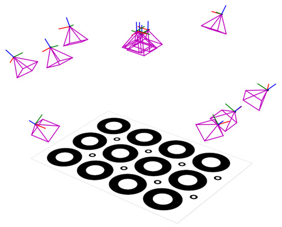
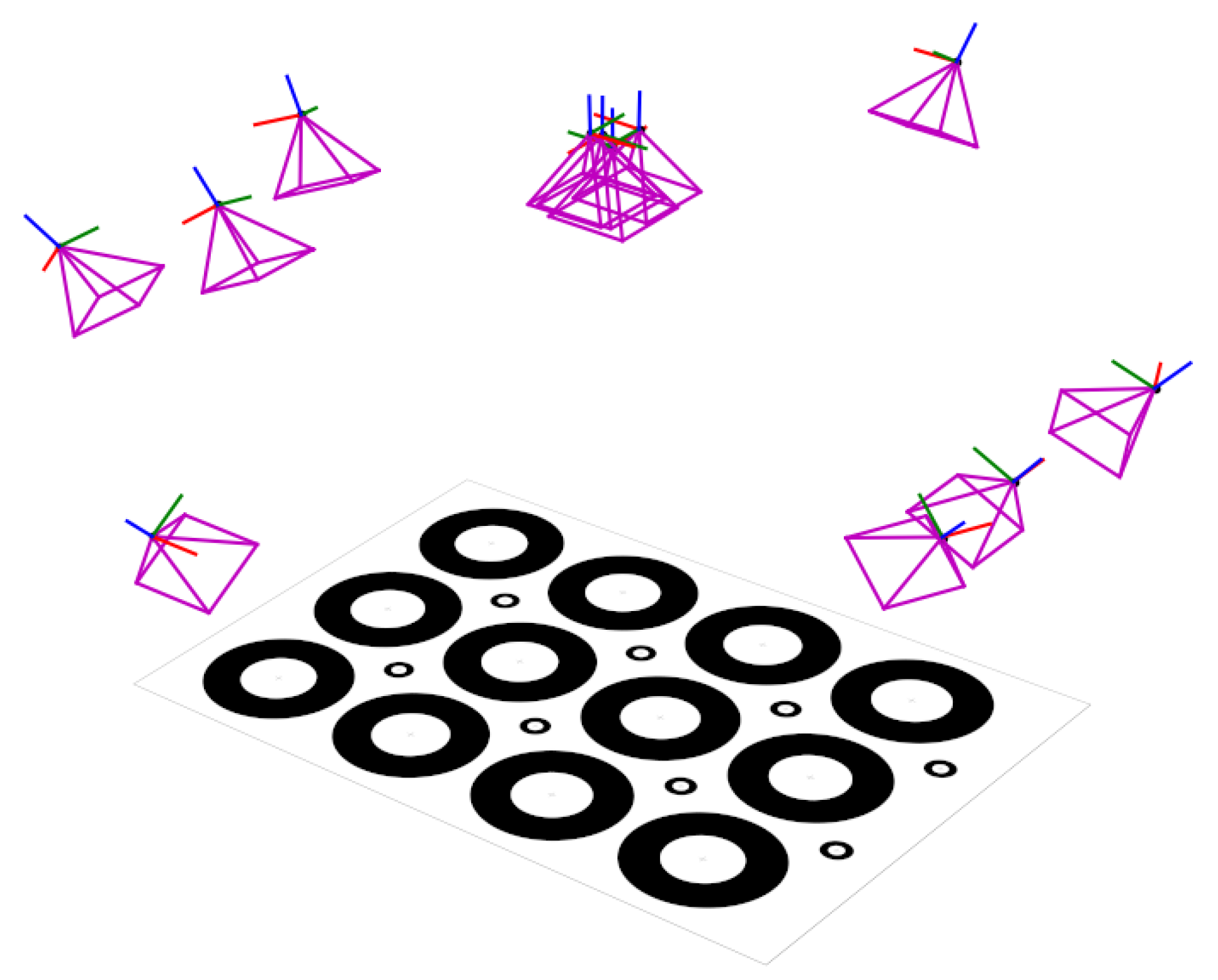
Twelve images were taken with an AVT Mako G-419C camera (Allied Vision Technologies, Nuremberg, Germany) (2048 × 2048 px, 5.5 µm pixel size) with a lens of 12 mm focal length. The image orientations are shown in Figure 7. The top-view images also followed a rotation strategy to de-correlate interior orientation parameters in self-calibration [23].

Initial values for the exterior orientation parameters in Figure 7 were obtained by spatial resections of each image, assuming an ideal distortion-free camera with a principal distance of 12 mm. The eccentricities reached values of up to 6 px for the inner rings and 23 px for the outer rings of the large concentric circle targets in the oblique images (computed with Equation (21)). Note that the target size was intentionally chosen to be large to highlight the effects of eccentricity and the gain of correction methods, knowing that the effects would be smaller in real applications with typically smaller target sizes.

Table 3. Minimum, maximum and mean major axis lengths of the image ellipses in the 12 images for the 12 larger and 8 smaller targets for the inner and outer rings.

		$2·{\mathit{R}}_{\mathit{C}}$	$\mathit{min}(2·\mathit{a})$	$\mathit{max}(2·\mathit{a})$	$\mathit{mean}(2·\mathit{a})$
larger targets, inner ring		30 mm	173 px	321 px	221 px
larger targets, outer ring		60 mm	347 px	646 px	444 px
smaller targets, inner ring		6 mm	34 px	68 px	44 px
smaller targets, outer ring		12 mm	69 px	138 px	89 px

provides information about the image scale, comparing the object and image target diameters. It shows the minimum, maximum and mean lengths of the image ellipse major axes for the twelve larger and eight smaller targets (inner and outer rings) of all images of the bundle.

5.1.2. Simulation

To check the algorithms and to estimate the influence of the eccentricity, noise-free simulations were performed with the different models. For each image, the image coordinates of the ellipse centers were computed with Equation (6), inserting the initial values of the exterior orientation parameters (Figure 7) and assuming a distortion-free lens with 12 mm principal distance. Furthermore, for each ellipse, a number of contour points were computed (to test the algorithm in Section 4.5). These image coordinates were then used as observations without additional artificial noise for a bundle adjustment (BA) with the different procedures shown in Section 4. The BA was computed as a free net adjustment where all circle centers were unknowns, as well as the exterior and interior orientation (including lens distortion parameters). Seven constraints were introduced for the free net adjustment:

$$\begin{array}{c}\hfill \sum _{i}d{\overrightarrow{X}}_{C,i}=\overrightarrow{0}\\ \hfill \sum _i{\overrightarrow{X}}_{C,i}\times d{\overrightarrow{X}}_{C,i}=\overrightarrow{0}\\ \hfill \sum _i{\overrightarrow{X}}_{C,i}^T·d{\overrightarrow{X}}_{C,i}=0\end{array}$$

(43)

where

• ${\overrightarrow{X}}_{C,i}$ = center of the i^th circle;
• $d{\overrightarrow{X}}_{C,i}$ = correction vector for ${\overrightarrow{X}}_{C,i}$ from BA.

Thirteen different scenarios were performed, as listed in

Table 4. Scenarios of bundle adjustments.

ID	Model	Input
$M_1$	Standard pinhole model w/o ecc. corr.	inner rings
$M_2$	Standard pinhole model w/o ecc. corr.	outer rings
$M_3$	Standard pinhole model with ecc. corr. in image space (Section 4.1, Equation (13))	inner rings
$M_4$	Standard pinhole model with ecc. corr. in image space (Section 4.1, Equation (13))	outer rings
$M_5$	Standard pinhole model with ecc. corr. in image space (Section 4.1, Equation (8))	inner rings
$M_6$	Standard pinhole model with ecc. corr. in image space (Section 4.1, Equation (8))	outer rings
$M_7$	Standard pinhole model with ecc. corr. in image space (Section 4.2, Equation (22))	both rings
$M_8$	Pinhole model for circles (Section 4.3)	inner rings
$M_9$	Pinhole model for circles (Section 4.3)	outer rings
$M_{10}$	Extended BA (model-side correction, Section 4.4)	inner rings
$M_{11}$	Extended BA (model-side correction, Section 4.4)	outer rings
$M_{12}$	BA with contour points (Section 4.5)	inner rings
$M_{13}$	BA with contour points (Section 4.5)	outer rings

. For six cases ($M_1$, $M_3$, $M_5$, $M_8$, $M_{10}$, $M_{12}$), only the ellipse centers and contour points of the inner rings of concentric circles were used as input; for another six cases ($M_2$, $M_4$, $M_6$, $M_9$, $M_{11}$, $M_{13}$), only the ellipse observations of the outer rings of concentric circles were used. Scenario $M_7$ works with the corrected image coordinates calculated with both rings (Section 4.2). In the cases of $M_{10}$, $M_{11}$, $M_{12}$ and $M_{13}$ (Section 4.4 and Section 4.5), the circles’ normals and radii were also introduced as unknowns.

The following quantities were used to evaluate the different methods:

• $RM{S}_{BA}$: RMS of the residuals of the image coordinates of the ellipse centers after BA to show the influence on the model fit (precision).
• c: estimated principal distance to show the influence on the main interior orientation parameter.
• $RM{S}_{ST\text{-}C}$: RMS of the residuals of the parameter estimation of a similarity transformation between the a priori and a posteriori circle centers to show the influence on the circle center coordinates.
• $RM{S}_{ST\text{-}P}$: RMS of the residuals of the parameter estimation of a similarity transformation between the a priori and a posteriori projection center coordinates to show the influence on the exterior orientation.

Algorithm 8 summarizes the procedure of the determination of the influence of the eccentricity error that was performed for the scenarios $M_1$ and $M_2$. Note that this procedure can also be applied to existing BAs to evaluate the influence of the eccentricity where the EOP, IOP, and circle parameters (centers, radii, normals) are used as input for Algorithm 8.

Algorithm 8 Determination of eccentricity influence of circular targets

Input:  Circle centers, radii and normals, EOP of an image bundle, IOP with or without lens-distortion. Compute the ellipse centers for each circle in each image using Equation (6). Perform a bundle adjustment with the standard pinhole model using the ellipse centers as observations. Compute reprojection error $RM{S}_{BA}$ to see the influence on the remaining model error. Estimate the least-squares similarity transformation parameters between the a priori and the a posteriori circle centers and consider the residuals’ RMS ($RM{S}_{ST\text{-}C}$). Estimate the least-squares similarity transformation parameters between the a priori and the a posteriori projection centers and consider the residuals’ RMS ($RM{S}_{ST\text{-}P}$). Output:  $RM{S}_{BA}$, $RM{S}_{ST\text{-}C}$, $RM{S}_{ST\text{-}P}$, further BA outputs.

Table 5. BA results of different models for simulations with 12 larger and 8 smaller concentric circles. n: number of observations, u: number of unknowns.

	n	u	${\mathit{RMS}}_{\mathit{BA}}$ in px	c in mm	${\mathit{RMS}}_{\mathit{ST}\text{-}\mathit{C}}$ in mm	${\mathit{RMS}}_{\mathit{ST}\text{-}\mathit{P}}$ in mm
$M_1$	480	142	0.169	12.039	0.149	0.594	inner rings
$M_2$	480	142	0.668	12.144	0.600	2.487	outer rings
$M_3$	480	142	0.089	12.000	0.020	0.162	inner rings
$M_4$	480	142	0.359	12.047	0.079	0.954	outer rings
$M_5$	480	142	0.000	12.000	0.000	0.000	inner rings
$M_6$	480	142	0.000	12.000	0.000	0.000	outer rings
$M_7$	480	142	0.002	12.000	0.001	0.004	both rings
$M_8$	480	142	0.000	12.000	0.000	0.000	inner rings
$M_9$	480	142	0.000	12.000	0.000	0.000	outer rings
$M_{10}$	960	222	0.000	12.000	0.000	0.000	inner rings
$M_{11}$	960	222	0.000	12.000	0.000	0.000	outer rings
$M_{12}$	15,360	222	0.000	12.000	0.000	0.000	inner rings
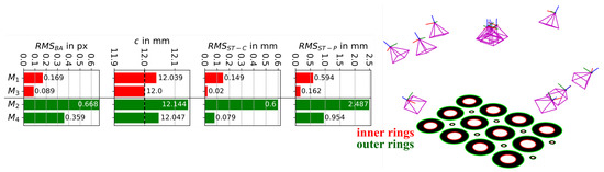
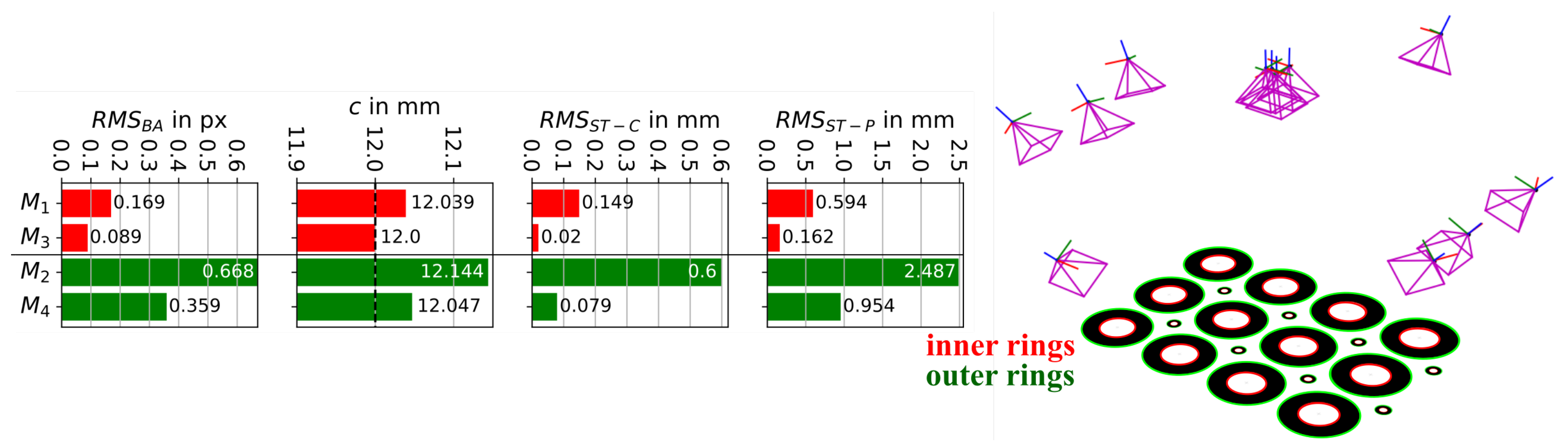
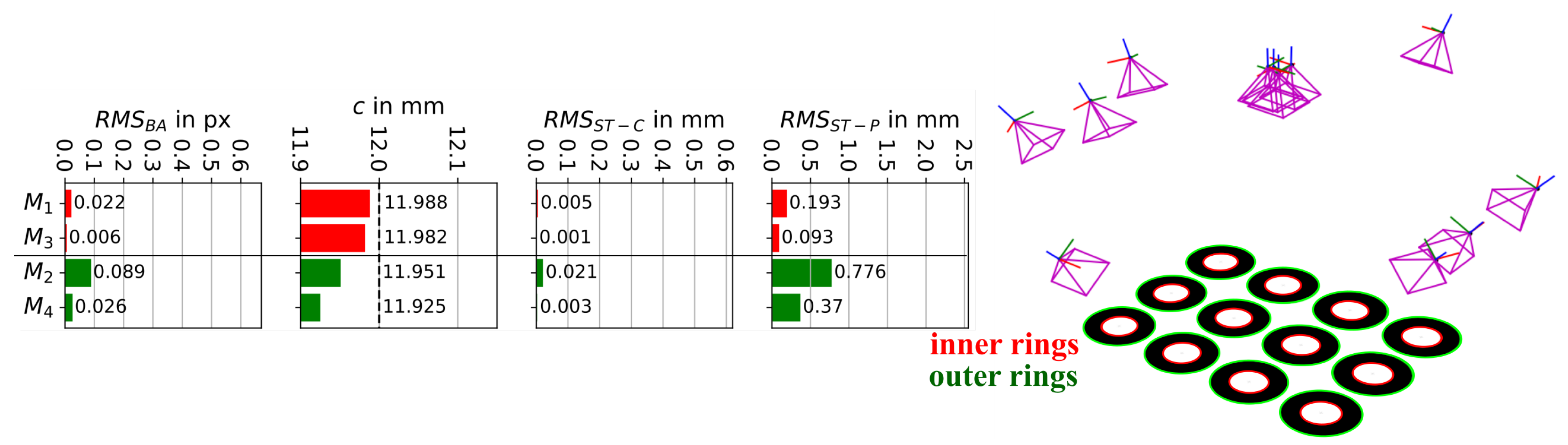
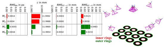
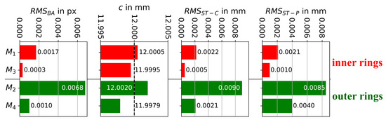
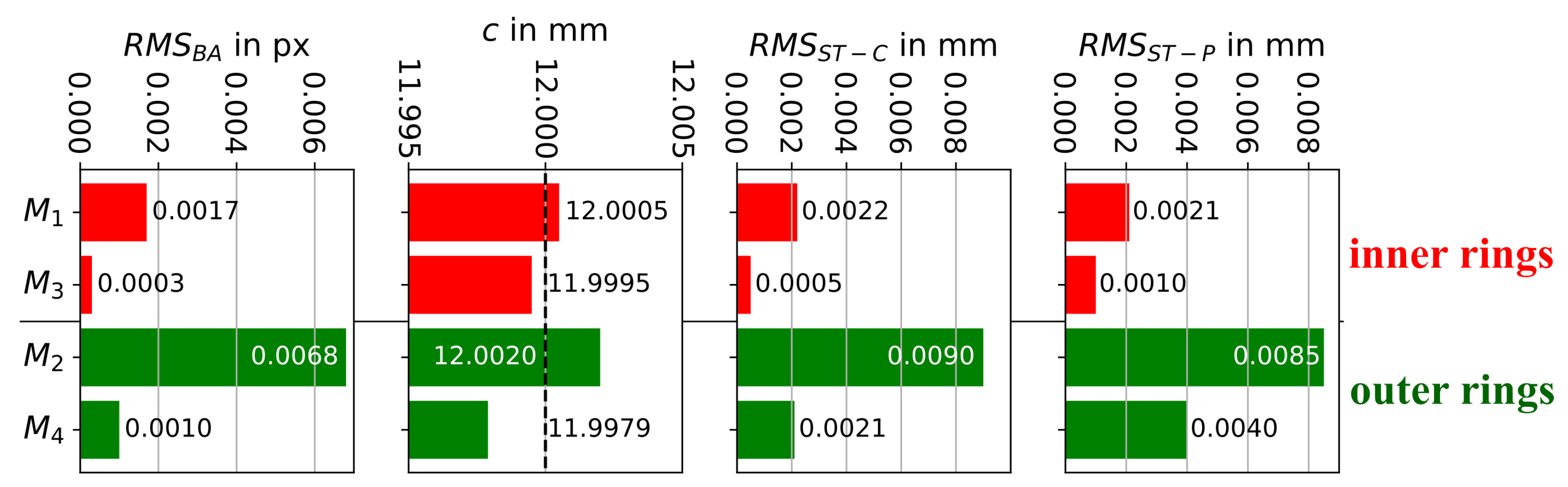
$M_{13}$	15,360	222	0.000	12.000	0.000	0.000	outer rings

shows the results of the different scenarios from Table 4, and Figure 8 depicts a reduced selection of the scenarios ($M_1$, $M_3$, $M_2$, $M_4$) where the errors due to eccentricity are fully or partially noticeable. Note that the arrangement of the scenarios in Figure 8 differs from the table to separate the analyses of the inner and outer rings in the bar plots. The bars of the analyses of the inner rings are colored red and for the outer rings are green. The standard pinhole model without eccentricity correction ($M_1$, $M_2$) showed the highest residuals of the image coordinates. The outer rings $M_2$ resulted in the highest deviations, with a four times higher $RM{S}_{BA}$ compared to the inner rings $M_1$ with half the radii. The effect on the interior orientation is revealed by the change in the principal distance c compared to the a priori value of 12 mm. The $RM{S}_{ST\text{-}C}$ of $M_1$ and $M_2$ was four times smaller than $RM{S}_{ST\text{-}P}$, which means that there was a higher influence on the exterior orientation than on the circle coordinates. Note that the largest distance between the projection center is only twice as large as the largest distance between the circle centers.

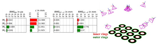
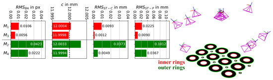
When the correction in image space with the approximated eccentricity was applied ($M_3$, $M_4$), the $RM{S}_{BA}$ was only halved and the other deviations were even smaller than half. However, the error could not be fully removed. Note that the ratio $R_C^2/Z_{C,cam}^2$ ranges from 0.002 and 0.005 for the inner rings of the twelve larger targets and for the outer rings ranges from 0.003 to 0.01, such that the condition $R_C^2\ll Z_{C,cam}^2$ is only partially fulfilled. Therefore, the exact correction terms ($M_5$, $M_6$) should be preferred. They, as well as the other correction models, resulted in zero deviations, showing that the models work perfectly. Note that no additional noise has been added in these simulations. Only $M_7$ shows a slight non-zero $RM{S}_{BA}$ of 0.002 px due to the approximation, but significantly smaller than $M_3$ and $M_4$. Some remaining errors in $M_3$ and $M_4$ seem to be eliminated by the coordinate difference calculation in $M_7$.

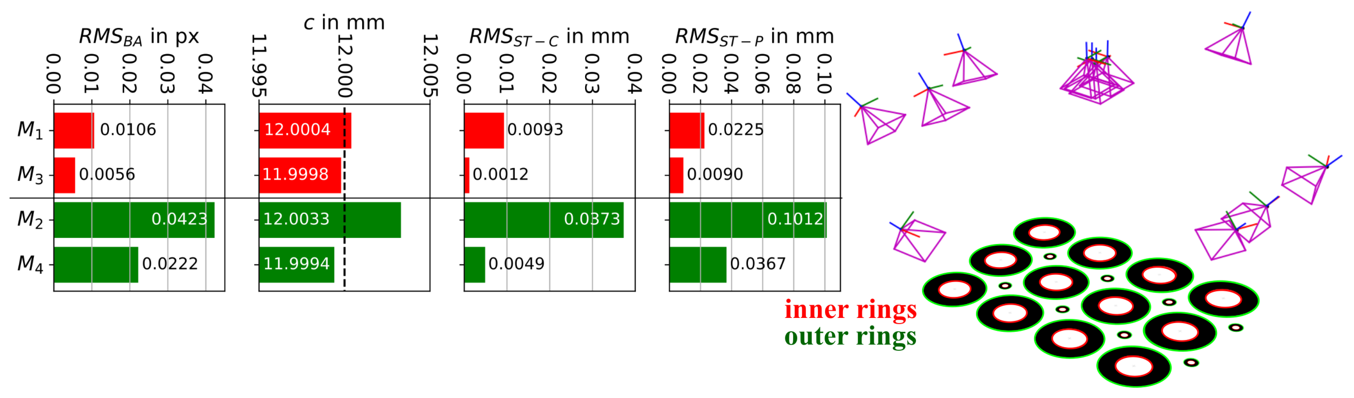
Different results were obtained when only the twelve large targets of equal size in Table 2 were used.

Table 6. BA results of different models with simulated image coordinates for the 12 larger equal-sized concentric circles. n: number of observations, u: number of unknowns.

	n	u	${\mathit{RMS}}_{\mathit{BA}}$ in px	c in mm	${\mathit{RMS}}_{\mathit{ST}\text{-}\mathit{C}}$ in mm	${\mathit{RMS}}_{\mathit{ST}\text{-}\mathit{P}}$ in mm
$M_1$	288	118	0.022	11.988	0.005	0.193	inner rings
$M_2$	288	118	0.089	11.951	0.021	0.776	outer rings
$M_3$	288	118	0.006	11.982	0.001	0.093	inner rings
$M_4$	288	118	0.026	11.925	0.003	0.370	outer rings
$M_5$	288	118	0.000	12.000	0.000	0.000	inner rings
$M_6$	288	118	0.000	12.000	0.000	0.000	outer rings
$M_7$	288	118	0.001	12.001	0.000	0.001	both rings
$M_8$	288	118	0.000	12.000	0.000	0.000	inner rings
$M_9$	288	118	0.000	12.000	0.000	0.000	outer rings
$M_{10}$	576	166	0.000	12.000	0.000	0.000	inner rings
$M_{11}$	576	166	0.000	12.000	0.000	0.000	outer rings
$M_{12}$	9216	166	0.000	12.000	0.000	0.000	inner rings
$M_{13}$	9216	166	0.000	12.000	0.000	0.000	outer rings

shows the results and Figure 9 shows a reduced selection of the scenarios $M_1$, $M_3$, $M_2$ and $M_4$. The deviations of the standard pinhole model without eccentricity correction ($M_1$, $M_2$) were significantly smaller here. The other scenarios behave similarly to the first simulation, but there was an underestimation of c without eccentricity correction (target value of c = 12 mm, shown as dashed line in Figure 9). The systematic eccentricity errors seem to be much better compensated by the exterior orientation parameters, as can also be seen in Figure 3.

It can be seen that the eccentricity error of circular targets on a planar test field should lead to much higher deviations when the targets are not of the same size. In the present case, this can be explained by correlations between target eccentricity parameters and camera exterior, as well as interior (incl. lens distortion) orientation parameters. This, however, only holds in the case of a planar target field and can thus not be generalized.

5.1.3. Bundle Adjustment with Real Image Measurements

In this section, the same scenarios of the simulations from the prior section were performed with the real image measurements. The star operator [20] was used to measure the image ellipse coordinates.

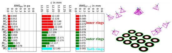
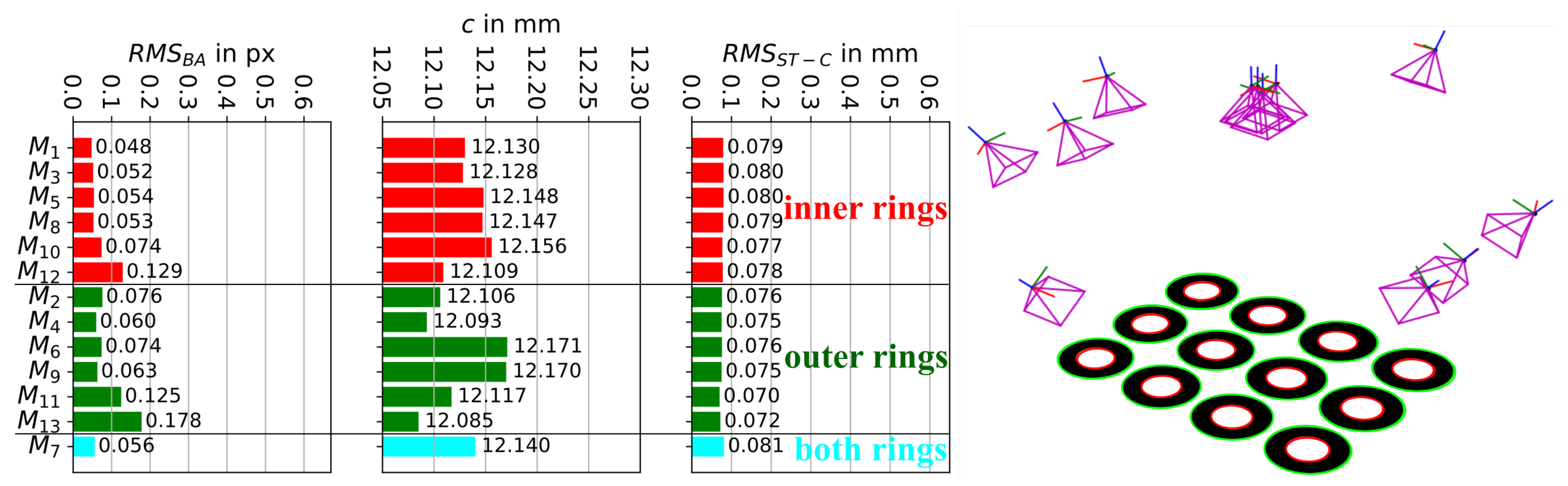
The results of the different BAs (as free net adjustments) with the 20 concentric circles in Figure 7 are shown in

Table 7. BA results of different models with 12 larger and 8 smaller concentric circles. n: number of observations, u: number of unknowns.

	n	u	${\mathit{RMS}}_{\mathit{BA}}$ in px	c in mm	${\mathit{RMS}}_{\mathit{ST}\text{-}\mathit{C}}$ in mm
$M_1$	480	142	0.168	12.175	0.172	inner rings
$M_2$	480	142	0.646	12.285	0.607	outer rings
$M_3$	480	142	0.098	12.143	0.075	inner rings
$M_4$	480	142	0.341	12.166	0.098	outer rings
$M_5$	480	142	0.057	12.149	0.071	inner rings
$M_6$	480	142	0.111	12.173	0.072	outer rings
$M_7$	480	142	0.055	12.142	0.072	both rings
$M_8$	480	142	0.055	12.148	0.071	inner rings
$M_9$	480	142	0.092	12.167	0.071	outer rings
$M_{10}$	960	222	0.067	12.161	0.070	inner rings
$M_{11}$	960	222	0.120	12.141	0.068	outer rings
$M_{12}$	19,980	222	0.114	12.123	0.070	inner rings
$M_{13}$	20,140	222	0.149	12.104	0.068	outer rings

and Figure 10. Again, the RMS of the image ellipse center residuals $RM{S}_{BA}$ after BA is shown as well as the principal distances and the RMS of the residuals of the parameter estimation of a similarity transformation between the a priori and a posteriori circle centers $RM{S}_{ST\text{-}C}$. The a priori circle centers can be assumed as target values, neglecting printing errors.

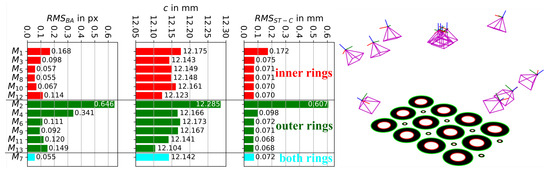
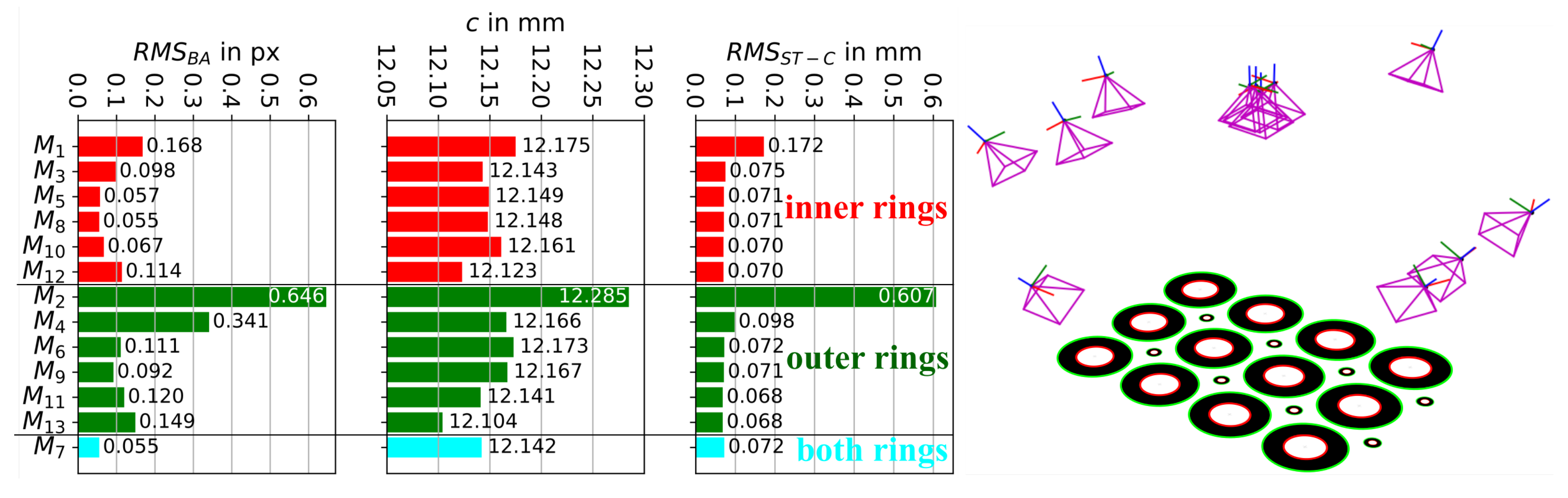
There is a high degree of consistency between the $RM{S}_{BA}$ as well as $RM{S}_{ST\text{-}C}$ of the simulation and the real image data. For the analysis of the inner rings, the $RM{S}_{BA}$ was 0.168 px without correction ($M_1$) and it was reduced to 0.057 px and 0.055 px with $M_5$ and $M_8$. The $RM{S}_{BA}$ of the extended BA ($M_{10}$) was slightly higher, with 0.067 px. For $M_{12}$ and $M_{13}$, there were higher $RM{S}_{BA}$ values than for $M_{10}$ and $M_{11}$, but note that $M_{12}$ and $M_{13}$ work with different observation data. The influence on the circle centers $RM{S}_{ST\text{-}C}$ was also reduced to almost one third compared to $M_1$.

For the inner rings (red bars in Figure 10), the principal distance c is also shown in Table 7, where $M_1$ yields the largest value (without eccentricity correction). When applying the eccentricity correction, the reduction in c was smaller, as expected from the simulations. The smallest c was computed for the BA with the contour points ($M_{12}$ and $M_{13}$). Note that some differences in c could be compensated by the radial-symmetric distortion parameters.

The error reduction for the outer rings was even stronger due to the quadratic error behavior. Considering the outer rings (green bars in Figure 10), the lowest $RM{S}_{BA}$ was 0.092 px with $M_9$ and also $RM{S}_{ST\text{-}C}$ was decreased to 0.07 mm. The differences of c were similar to the simulations (decrease of 0.14 mm). The correction with both rings $M_7$ reached an $RM{S}_{BA}$ of 0.055 px and an $RM{S}_{ST\text{-}C}$ of 0.07 mm. Thus, it was similar to the other methods.

Note that the expectation value for the principal distance c does not correspond to the 12 mm focal length here, as the camera was not focused to infinity.

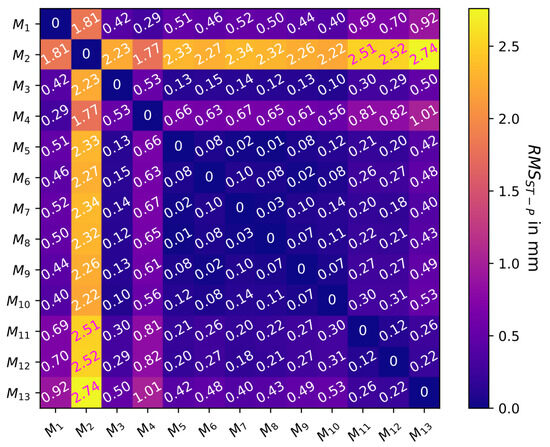
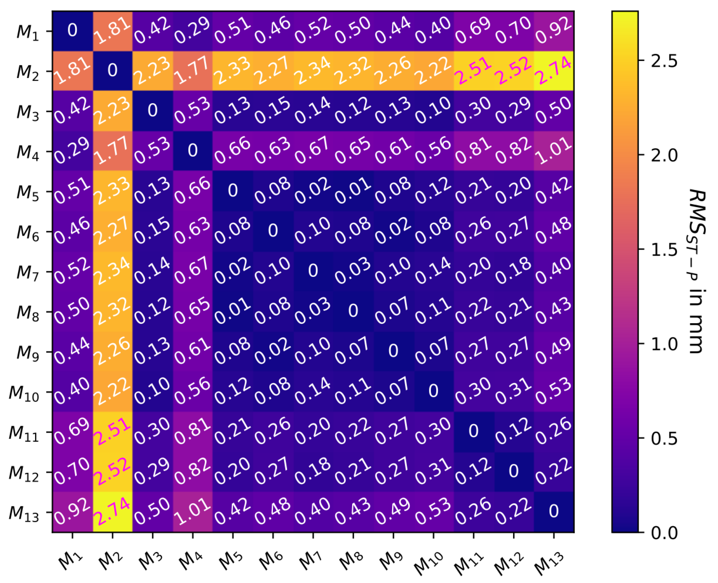
In contrast to the simulations, Table 7 and Figure 10 do not show the RMS of the residuals of the similarity transformation of the projection centers $RM{S}_{ST\text{-}P}$ because the exact projection centers are not known. However, the $RM{S}_{ST\text{-}P}$ of the similarity transformation between the projection center results of the different scenarios can be computed for each combination. Figure 11 shows a heatmap with the RMS values. The smallest RMS values, and thus the smallest differences in the projection center results, occur between the scenarios where corrections were applied. The largest errors are visible in the second column because $M_2$ was computed with the outer rings of the targets and without eccentricity correction. This is obvious due the highest eccentricity effects for the larger radii. The first column shows significantly smaller values. Remarkable is also the high $RM{S}_{ST\text{-}P}$ of 1.81 mm between $M_1$ and $M_2$, both without corrections, which shows the effect of the higher eccentricity for the larger radius. This value fits with the difference between $M_1$ and $M_2$ in the simulation (≈1.9 mm). The RMS values in the second column with values (other than $M_4$) of 2.22 to 2.74 mm also fit with the simulation, where the $RM{S}_{ST\text{-}P}$ was 2.5 mm for the outer rings without ecc. corr.

As in the simulation in the previous subsection, the case of only equal-sized targets was considered by using only the twelve large targets in Table 2—see

Table 8. BA results of different models for the 12 larger equal sized concentric circles. n: number of observations, u: number of unknowns.

	n	u	${\mathit{RMS}}_{\mathit{BA}}$ in px	c in mm	${\mathit{RMS}}_{\mathit{ST}\text{-}\mathit{C}}$ in mm
$M_1$	288	118	0.048	12.130	0.079	inner rings
$M_2$	288	118	0.076	12.106	0.076	outer rings
$M_3$	288	118	0.052	12.128	0.080	inner rings
$M_4$	288	118	0.060	12.093	0.075	outer rings
$M_5$	288	118	0.054	12.148	0.080	inner rings
$M_6$	288	118	0.074	12.171	0.076	outer rings
$M_7$	288	118	0.056	12.140	0.081	both rings
$M_8$	288	118	0.053	12.147	0.079	inner rings
$M_9$	288	118	0.063	12.170	0.075	outer rings
$M_{10}$	576	166	0.074	12.156	0.077	inner rings
$M_{11}$	576	166	0.125	12.117	0.070	outer rings
$M_{12}$	12,004	166	0.129	12.109	0.078	inner rings
$M_{13}$	12,076	166	0.178	12.085	0.072	outer rings

and Figure 12. For the inner rings, there was even a slight increase in $RM{S}_{BA}$ when the correction models were applied ($M_3$, $M_5$, $M_8$, $M_{10}$) compared to the case without eccentricity correction ($M_1$). Considering the outer rings, there was a slight reduction in the $RM{S}_{BA}$ values ($M_4$, $M_6$, $M_9$) compared to $M_2$ (without eccentricity correction). $M_{11}$ yielded a larger $RM{S}_{BA}$. The BAs with the contour points ($M_{12}$ and $M_{13}$) had the largest $RM{S}_{BA}$ due to the different observation data. For the inner rings, the estimated principal distances of $M_5$, $M_8$ and $M_{10}$ showed an increase that was slight larger than in the simulation and $M_3$ showed almost no change to $M_1$. The changes of c are better visible for the outer rings, where $M_4$ and $M_6$ showed an increase of 0.065 mm compared to $M_2$, which fits well with the simulation (≈0.05 mm). $M_4$ showed an decrease of around 0.01 mm compared to $M_2$—a smaller reduction than the simulation. The increase in $c_{M11}$ was significantly smaller than for $M_4$ and $M_6$. $c_{M7}$ lay between $c_{M1}$ and $c_{M5}$. Also here, the BAs with contour points ($M_{12}$ and $M_{13}$) showed a different behavior, with a reduction in c that does not fit with the simulations.

The RMS of the similarity transformations of the circle centers $RM{S}_{ST\text{-}C}$ did not show significant changes for the inner rings. Considering the outer rings, only $M_{11}$ and $M_{13}$ showed a slight reduction in $RM{S}_{ST\text{-}C}$ compared to $M_2$ (0.06 mm and 0.04 mm), values that were larger than in the simulation (0.02 mm). Over all, the results match the simulation, where also only small changes were revealed for these three quantities.

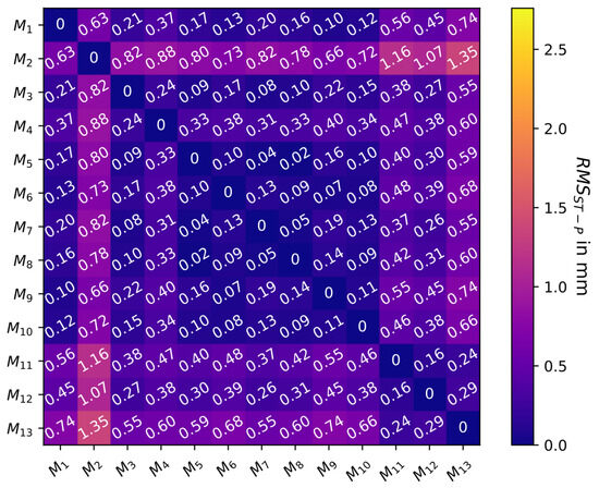
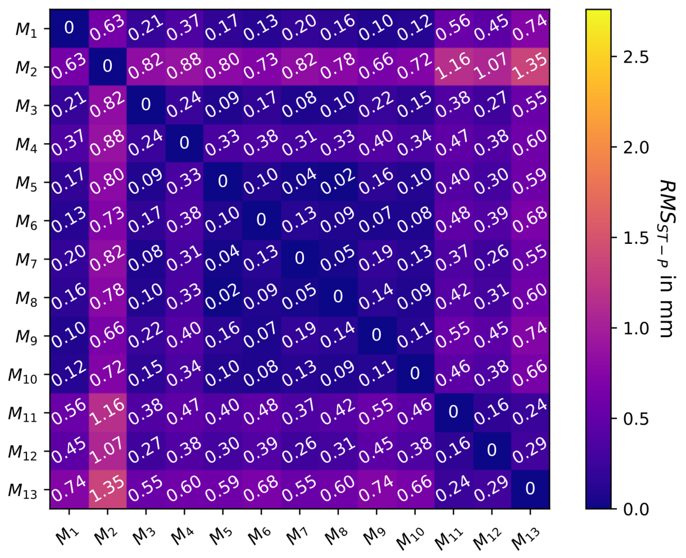
The $RM{S}_{ST\text{-}P}$ values were not computed in Table 8 due to the unknown target values of the exterior orientation parameters, where larger deviations would be expected. However, a heatmap with the $RM{S}_{ST\text{-}P}$ between all scenarios of BA can be computed, as shown in Figure 13. The values are significantly smaller than in Figure 11. Again, the second column shows the largest values because $M_2$ works without eccentricity correction for the outer rings and thus has the biggest influence on the exterior orientation. The $RM{S}_{ST\text{-}P}$ in the second column range from 0.66 mm to 0.88 mm ($M_2$ until $M_{10}$), which fits well with the simulation, where the corrections reduced the RMS by 0.78 mm. Also, the $RM{S}_{ST\text{-}P}$ of 0.63 mm between $M_1$ and $M_2$ fits well with the difference of 0.58 mm (0.776 mm–0.193 mm) in the simulation. The last three values of the second column show higher RMS values (>1 mm), which exceed the values from the simulation. The first column shows the differences between the projection centers and the scenario without eccentricity correction for the inner rings. $M_5$ and $M_8$ (BA for inner rings with ecc. corr.) yielded RMS values of 0.17 mm and 0.16 mm, which are slightly smaller but similar to the simulation (0.193 mm). $M_{10}$ showed a smaller RMS of 0.12 mm and $M_{12}$ showed a significantly larger RMS of 0.45 mm. Between the scenarios with eccentricity correction, there are still remaining errors. In particular, the last three rows ($M_{11}$, $M_{12}$ and $M_{13}$) show high RMS and thus larger differences in the projection centers than the other scenarios. As one can see from the results, a more complex solution of a bundle adjustment based on a number of ellipse contour points does not lead to an improvement in the results.

Overall, the real image data experiments with the planar test field confirm the simulation results, where there were higher compensation effects by IOP, EOP and circle centers for test fields with equal-sized targets than for the test field with different-sized targets. The behavior was also found to be similar for spherical targets, as shown in [24].

5.1.4. Bundle Adjustment Simulation with Four Times Smaller Target Radii

Further simulations were performed for the same image configuration and modified test field with smaller radii. The radii were reduced by a factor of four compared to Section 5.1.2. This was done to analyze a more practical case with a smaller image scale for the targets and, in addition, because the condition $R_C^2\ll Z_{C,cam}^2$ is better fulfilled. The radii of the inner rings of the twelve larger targets were 3.75 mm, and 7.5 mm for the outer rings. The eight smaller targets had radii of 0.75 mm for the inner rings and 1.5 mm for the outer rings in this simulation. Thus, the ellipse major axis lengths were in a range of 43 to 80 px for the inner ring radii of the twelve larger targets ($R_C^2/Z_{C,cam}^2\in (4·{10}^{-6},3·{10}^{-4})$ for the inner rings).

Figure 14 shows the results of the simulated bundle with twelve larger and eight smaller targets. The RMS values are significantly smaller, compared to those in Section 5.1.2. The $RM{S}_{BA}$ was 16 (=4²) times smaller. Also, in this case, the approximate eccentricity correction in image space ($M_3$, $M_4$) reduces the $RM{S}_{BA}$ by half compared to the computation without eccentricity correction ($M_1$, $M_2$). The behavior is similar for $RM{S}_{ST\text{-}C}$. It was also reduced by factor of 16 compared to Section 5.1.2. As for the larger radii, the approximate eccentricity correction ($M_3$, $M_4$) reduced the $RM{S}_{ST\text{-}C}$ (factor 7–8). The decrease in $RM{S}_{ST\text{-}P}$ was stronger: it was 25 times smaller than in Section 5.1.2. The reduction in $RM{S}_{ST\text{-}P}$ between without correction and approximate correction slightly differs from Section 5.1.2. The differences between the estimated principal distances and the target value of 12 mm were significantly smaller compared to Section 5.1.2.

We also considered the case where only the twelve larger targets were analyzed; see Figure 15. $RM{S}_{BA}$ and $RM{S}_{ST\text{-}C}$ were also 16 (=4²) times smaller compared to Section 5.1.2. The reduction factor is also 16 for $RM{S}_{ST\text{-}P}$. Between without correction ($M_1$, $M_2$) and approximate correction ($M_3$, $M_4$), the decreasing factor remains at two for $RM{S}_{ST\text{-}P}$ and remains at three to four for $RM{S}_{BA}$.

5.2. Experiment Using a Non-Planar Test Field

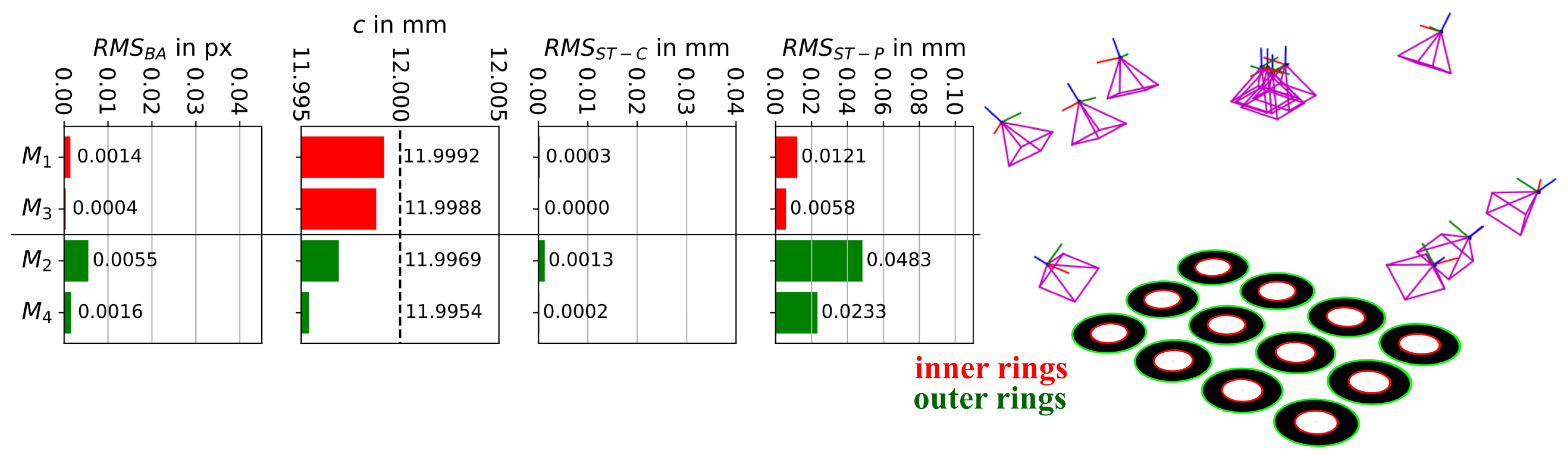
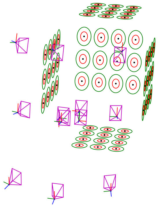
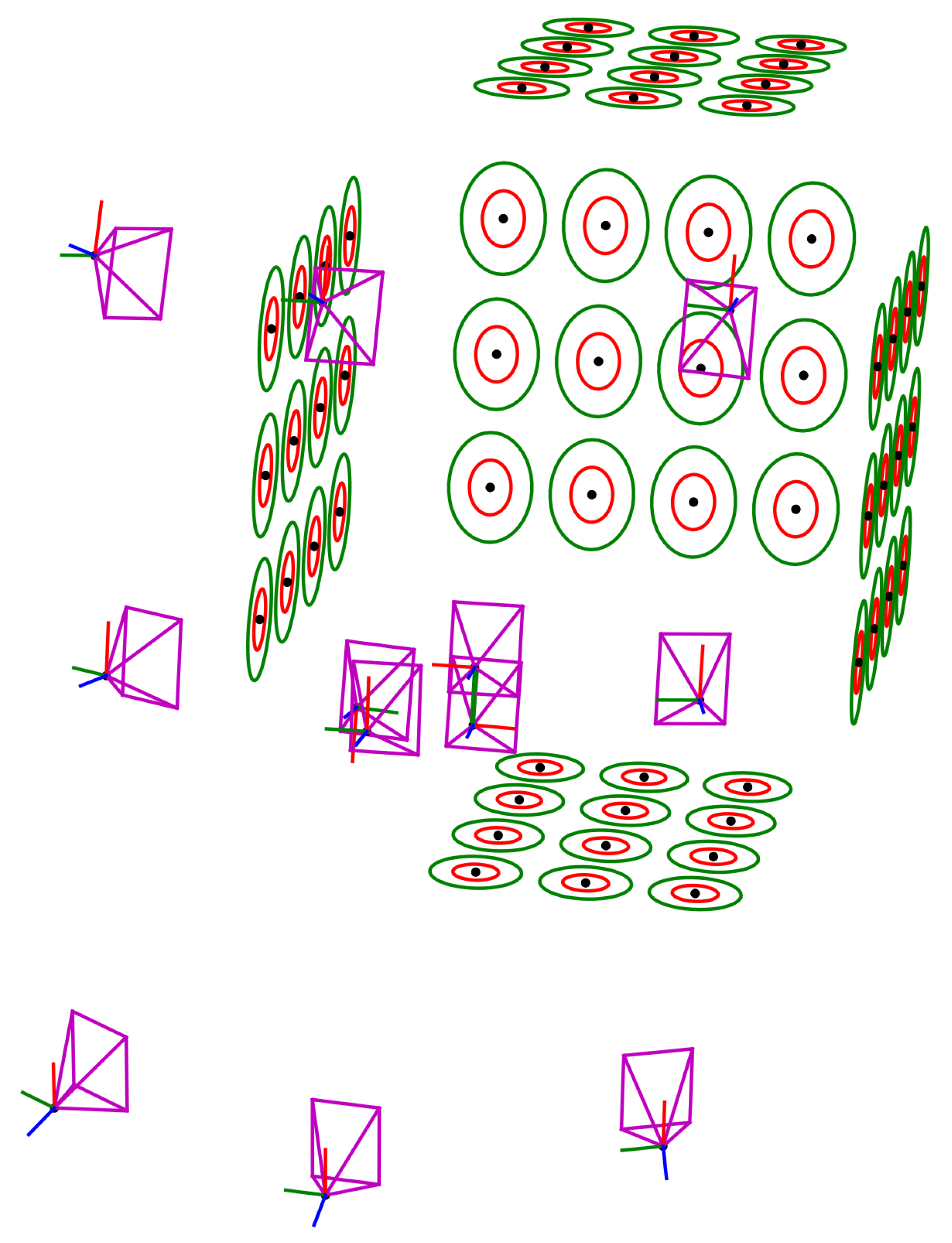
While the former section dealt with a planar test field, this section deals with a real image data experiment using a non-planar test body. This test object comes with a large variety of circle normal directions, and the 3D character causes less correlation between parameters. The field was equipped with 60 equal-sized concentric circle targets (with target radii $R_{C,i}$ = 13 mm and $R_{C,o}$ = 26 mm), 12 in each of five perpendicular planes. The test field had a size of ca. (34 cm)³. Again, a bundle of twelve images was recorded. The four rotated images in the center of the bundle contained all targets, while in each of the oblique-view images only a part of the targets was visible. The images in the corner of the bundle contained 36 targets; the other ones contained 48. Figure 16 shows a 3D plot of the test field as well as the image orientations. In this experiment, the same camera was used as in Section 5.1.

In order to evaluate the image scale,

Table 9. Minimum, maximum and mean major axis lengths of the image ellipses in the 12 images for the inner and outer rings of the targets.

	$2·{\mathit{R}}_{\mathit{C}}$	$\mathit{min}(2·\mathit{a})$	$\mathit{max}(2·\mathit{a})$	$\mathit{mean}(2·\mathit{a})$
inner rings	26 mm	72 px	136 px	96 px
outer rings	52 mm	144 px	275 px	193 px

compares the object and image diameters of the targets. It shows the minimum, maximum and mean lengths of the image ellipse major axes for the inner and outer rings of the targets of all images of the bundle ($R_C^2/Z_{C,cam}^2\in (2.7·{10}^{-4},1.3·{10}^{-3})$ for the inner rings).

5.2.1. Simulation

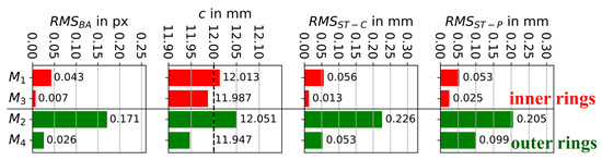
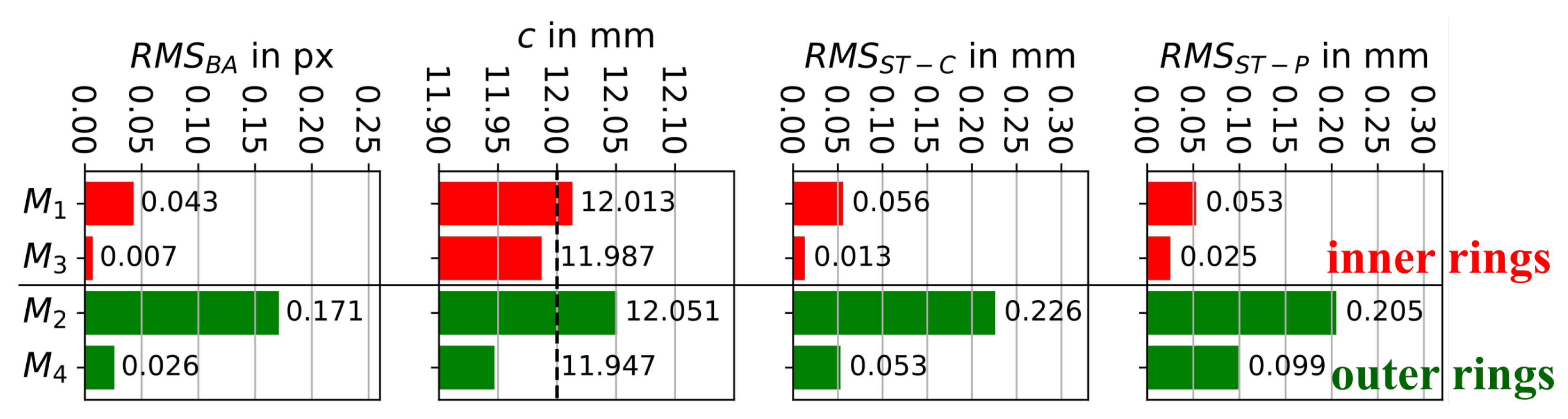
As in the experiments with the planar test field, the bundle adjustments were first computed for the different models with simulated image coordinates. The image coordinates (ellipse centers) and contour points were calculated with the approximate circle centers, exterior orientation parameters and a lens-distortion-free lens of 12 mm. These simulated observations and the predetermined orientation parameters were then used as input for the bundle adjustments.

Table 10. BA results of different models with simulated image coordinates for the non-planar test field of concentric circles. n: number of observations, u: number of unknowns.

	n	u	${\mathit{RMS}}_{\mathit{BA}}$ in px	c in mm	${\mathit{RMS}}_{\mathit{ST}\text{-}\mathit{C}}$ in mm	${\mathit{RMS}}_{\mathit{ST}\text{-}\mathit{P}}$ in mm
$M_1$	1150	262	0.043	12.013	0.056	0.053	inner rings
$M_2$	1150	262	0.171	12.051	0.226	0.205	outer rings
$M_3$	1150	262	0.007	11.987	0.013	0.025	inner rings
$M_4$	1150	262	0.026	11.947	0.053	0.099	outer rings
$M_5$	1150	262	0.000	12.000	0.000	0.000	inner rings
$M_6$	1150	262	0.000	12.000	0.000	0.000	outer rings
$M_7$	1150	262	0.000	12.000	0.000	0.000	both rings
$M_8$	1150	262	0.000	12.000	0.000	0.000	inner rings
$M_9$	1150	262	0.000	12.000	0.000	0.000	outer rings
$M_{10}$	2300	502	0.000	12.000	0.000	0.000	inner rings
$M_{11}$	2300	502	0.000	12.000	0.000	0.000	outer rings
$M_{12}$	24,150	502	0.000	12.000	0.000	0.000	inner rings
$M_{13}$	24,150	502	0.000	12.000	0.000	0.000	outer rings

shows the results. Again, the first two rows show the values without eccentricity correction delivering the highest RMS values, especially in the second row, where the outer rings were used (four times larger than for inner rings). The reprojection error $RM{S}_{BA}$ was 0.043 px for the inner rings ($M_1$) and 0.171 px for the outer rings ($M_2$). The estimated principal distances were larger ($c_{M1}$ = 12.013 mm and $c_{M2}$ = 12.051 mm) than the given (a priori) c of 12 mm, which shows the effect of partial error compensation by the interior orientation parameters. Using the approximate correction method ($M_3$ and $M_4$), the errors were reduced significantly. The other methods show zero deviations from the given parameters, resulting in zero errors for $RM{S}_{BA}$, $RM{S}_{ST\text{-}C}$, and $RM{S}_{ST\text{-}P}$, proving that the correction methods worked well. The bar plots in Figure 17 depict a reduced representation of Table 10, where only the first methods are shown and the order was changed so that, first, the results of the inner rings are shown in red. The results of the outer rings are depicted in green.

5.2.2. Bundle Adjustment with Real Image Measurements

This subsection shows the results of the bundle adjustments of the different methods with the real image measurements; see

Table 11. BA results of different models for the non-planar test field of concentric circles. n: number of observations, u: number of unknowns.

	n	u	${\mathit{RMS}}_{\mathit{BA}}$ in px	c in px
$M_1$	1150	262	0.072	12.124	inner rings
$M_2$	1150	262	0.194	12.161	outer rings
$M_3$	1150	262	0.057	12.098	inner rings
$M_4$	1150	262	0.100	12.053	outer rings
$M_5$	1150	262	0.056	12.111	inner rings
$M_6$	1150	262	0.096	12.107	outer rings
$M_7$	1150	262	0.065	12.112	both rings
$M_8$	1150	262	0.056	12.111	inner rings
$M_9$	1150	262	0.096	12.107	outer rings
$M_{10}$	2300	502	0.056	12.110	inner rings
$M_{11}$	2300	502	0.096	12.104	outer rings
$M_{12}$	47,798	502	0.091	12.108	inner rings
$M_{13}$	48,198	502	0.159	12.100	outer rings

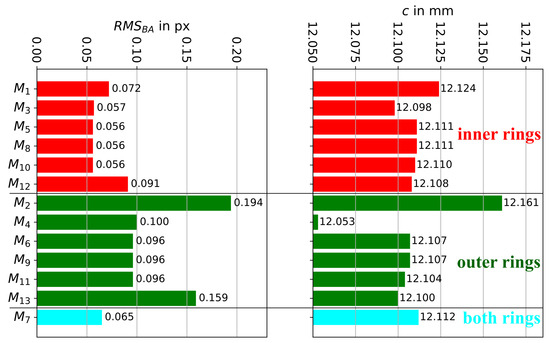
and Figure 18.

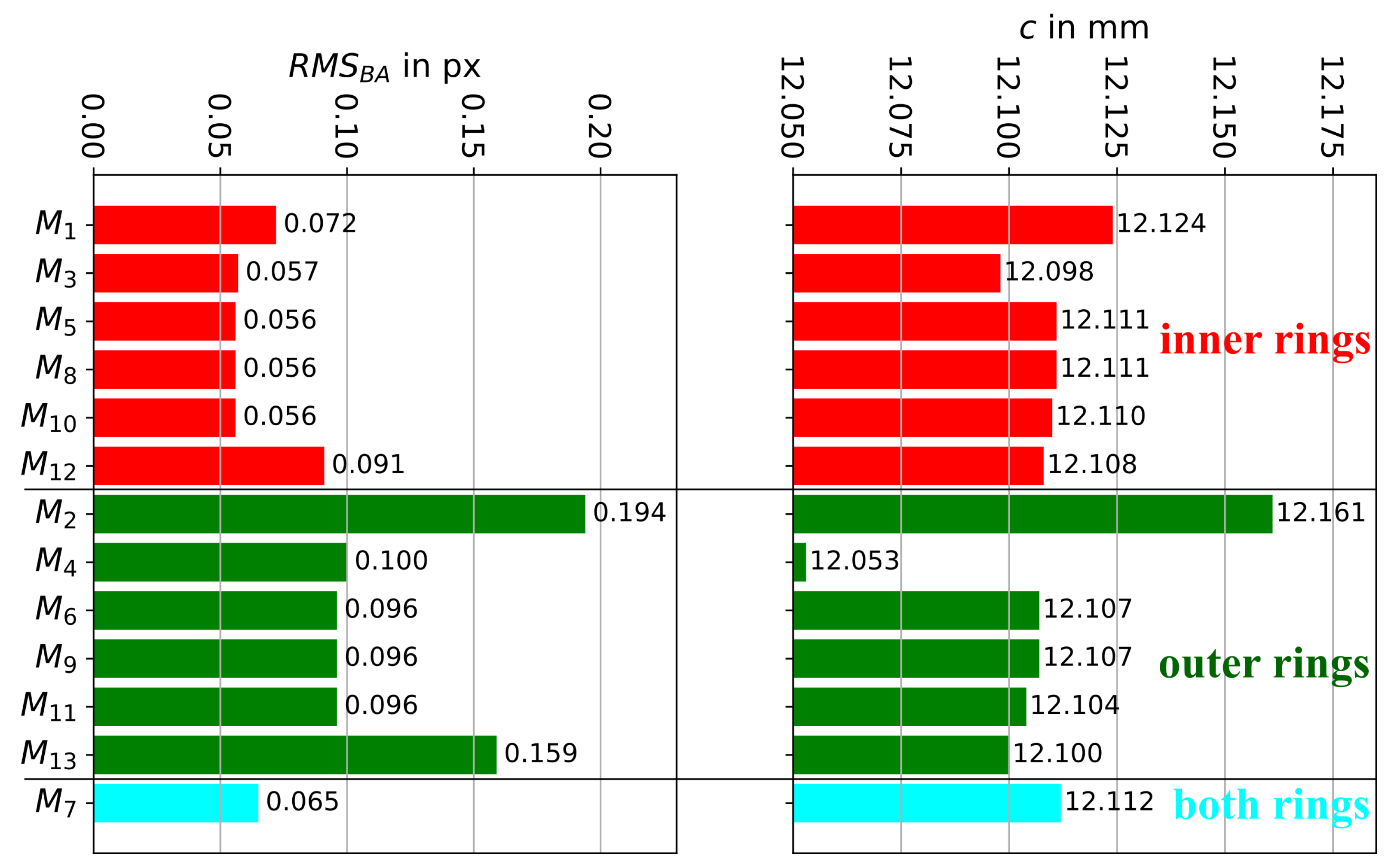
Without eccentricity correction ($M_1$ and $M_2$), the reprojection error was 0.072 px for the inner rings and 0.194 px for the outer rings. For the approximate correction method in the image space ($M_3$ and $M_4$), the $RM{S}_{BA}$ was decreased by 21% for the inner rings and by almost 50% for the outer rings. There were slightly smaller values for the exact correction term in the image space ($M_5$ with 0.056 px and $M_6$ with 0.96 px), such that the values fell below those in the simulation: $RM{S}_{BA,M1}-RM{S}_{BA,M5}$ = 0.16 px $<RM{S}_{BA,M1,sim}$ = 0.043 px and $RM{S}_{BA,M2}-RM{S}_{BA,M6}$ = 0.98 px $<RM{S}_{BA,M2,sim}$ = 0.171 px. For the concentric circle correction ($M_7$), the $RM{S}_{BA}$ is between the values for $M_3$/$M_5$ and $M_1$ (without correction). For the method with model adaption (inner rings: $M_8$ and $M_{10}$; outer rings: $M_9$ and $M_{11}$), the $RM{S}_{BA}$ values were equal to the exact image space correction ($M_5$ and $M_6$). For the bundle adjustments with the contour points ($M_{12}$ and $M_{13}$), the $RM{S}_{BA}$ values were larger than without correction ($M_1$ and $M_2$), which may be caused by a different model and a different number of observations. All in all, the reduction in $RM{S}_{BA}$ by the correction methods was smaller than in the simulations but showed a positive effect on the reprojection error.

Considering the principal distance c, the behavior is similar to the simulation. Without eccentricity correction ($M_1$ and $M_2$) produced the largest c values. The smallest c values were obtained by the approximate eccentricity correction in the image space ($M_3$ and $M_4$). The other correction methods yielded c values in between, with differences to $M_1$ and $M_2$ that are well-suited to the simulation. This shows the eccentricity compensation effect of the inner orientation parameter c.

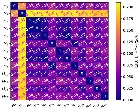
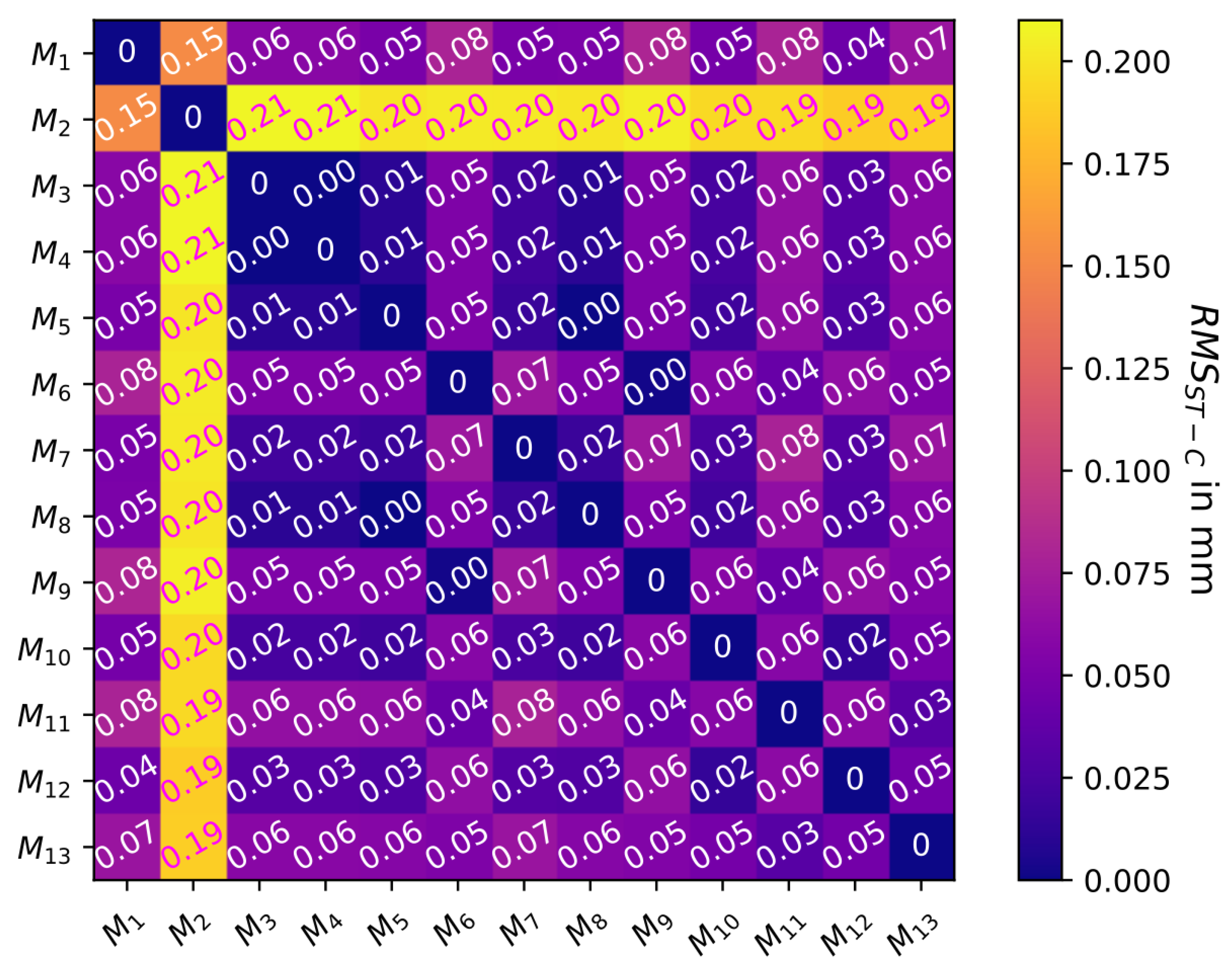
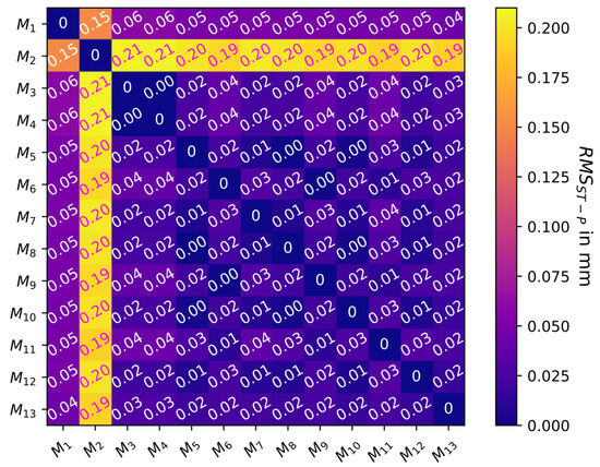
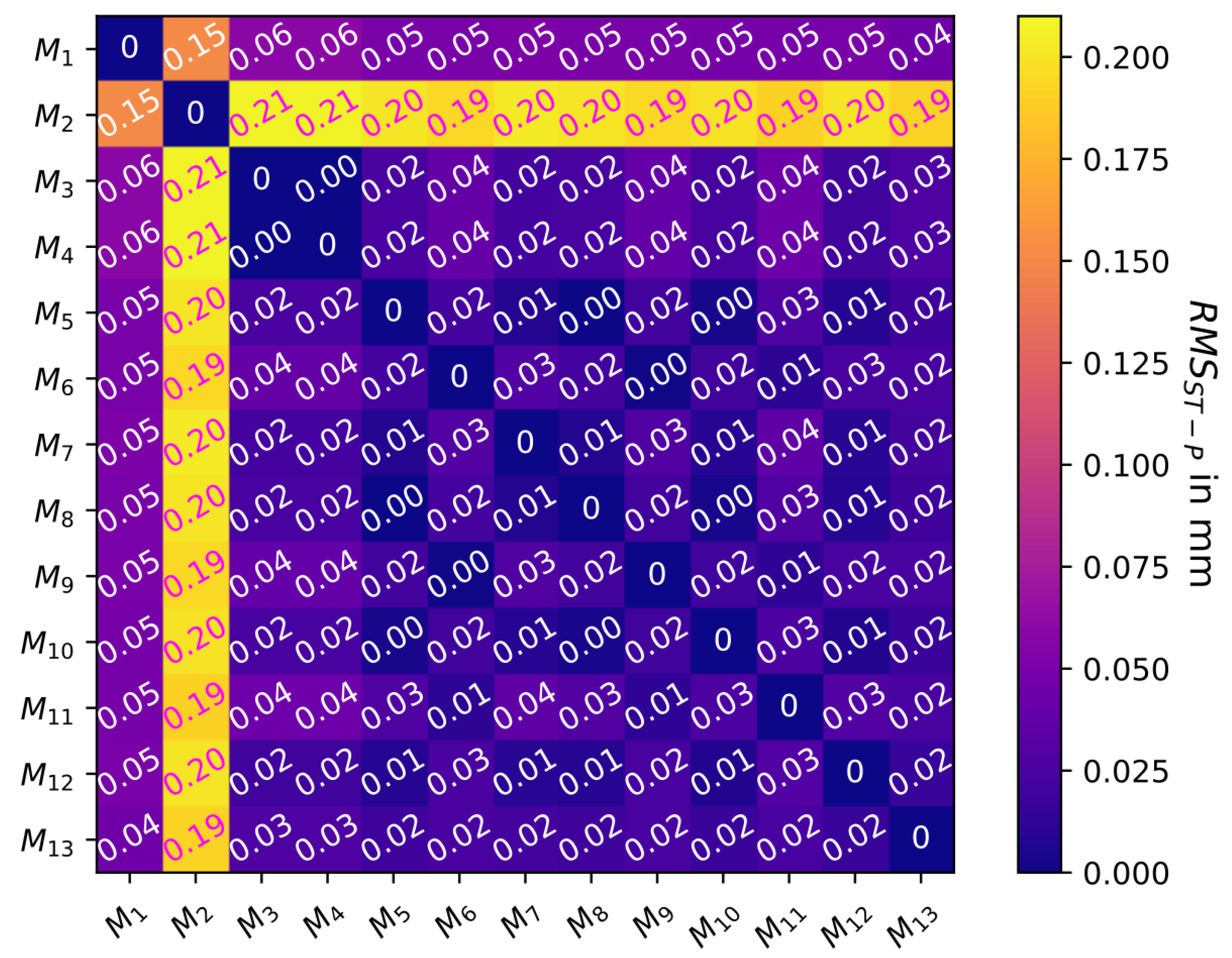
Table 11 and Figure 18 do not show the $RM{S}_{ST\text{-}C}$ and $RM{S}_{ST\text{-}P}$, as there are no reference values of the circle and projection centers for the non-planar test field. Instead, Figure 19 and Figure 20 show the $RM{S}_{ST\text{-}C}$ and $RM{S}_{ST\text{-}P}$ between the adjusted results of the bundle adjustments of the different models as heat maps. Here, similarity transformations were computed between each combination of the different method results for the circle and projection centers. The second columns in both matrices show the largest values (≈0.2 mm) due the largest eccentricities of the outer rings without correction. These values fit to the $RM{S}_{ST\text{-}C}$ and $RM{S}_{ST\text{-}P}$ of the simulations, where the reductions in the correction methods were 0.226 mm and 0.205 mm. The first columns show the differences of the correction methods compared to $M_1$ (without eccentricity correction). There, the $RM{S}_{ST\text{-}C}$ values range from 0.04 to 0.06 mm for the inner rings ($M_3$, $M_5$, $M_8$, $M_{10}$, $M_{12}$ and in addition $M_7$), which also fits with the reduction of the simulation of 0.05 mm for the inner rings. For the correction method for the outer rings ($M_4$, $M_6$, $M_9$, $M_{11}$, $M_{13}$), the $RM{S}_{ST\text{-}C}$ values range from 0.06 to 0.08 mm, which could be caused by the larger target radii and other influences. For the $RM{S}_{ST\text{-}P}$ values (Figure 20), the behavior was similar with a smaller range.

5.2.3. Bundle Adjustment Simulation with Five Times Smaller Target Radii

The simulation in Section 5.2.1 was also done with five times smaller radii so that the ellipse major axes’ lengths were smaller than 30 px for the inner rings of the targets. Thus, $R_C^2\ll Z_{C,cam}^2$ is rather fulfilled ($R_C^2/Z_{C,cam}^2\in (1·{10}^{-5},5·{10}^{-5})$ for the inner rings). Figure 21 shows the remaining errors after the bundle adjustments for the scenarios without eccentricity correction ($M_1$, $M_2$) and with the approximate eccentricity correction in the image space ($M_3$, $M_4$). Compared to Section 5.2.1, the RMS values ($RM{S}_{BA}$, $RM{S}_{ST\text{-}C}$$RM{S}_{ST\text{-}P}$) were reduced by a factor of 25 = 5². The reduction factors between the scenarios without eccentricity correction and with the approximate eccentricity correction remained at the values from Section 5.2.1: 6–7 for $RM{S}_{BA}$, 4–5 for $RM{S}_{ST\text{-}C}$ and 2 for $RM{S}_{ST\text{-}P}$. For this scenario, the errors are so small that they have no impact.

6. Scale Definition by Radii of Circles

As shown in Section 4.4 and Section 4.5, the radii of the circles are part of the model that can either be introduced as unknowns or be used as constants, as they are often known in practice. Therefore, they can also be used to define the scale.

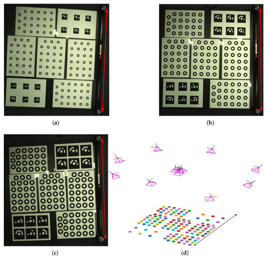
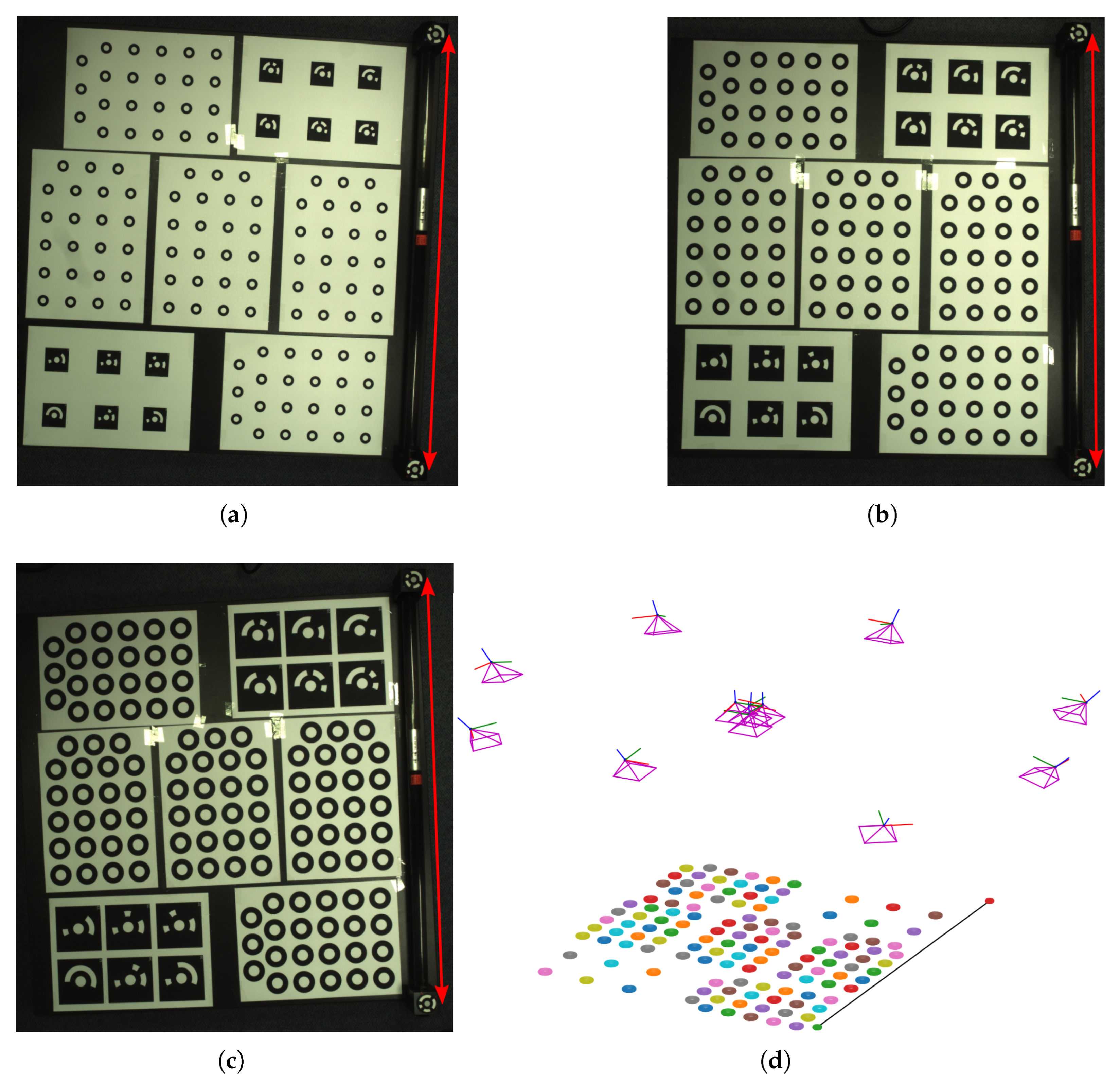
In order to investigate the precision and accuracy of the scale definition by known radii of circular targets, three similar test fields with different target radii (5 mm, 7.5 mm and 10 mm, externally verified), each endued with a scale bar (reference length: 740.289 mm), were used—see Figure 22a–c. The planar test fields had a dimension of ca. 70 × 75 cm². For each test field, a bundle of twelve images was recorded, as illustrated in Figure 22d using an AVT Alvium 1800 U-2040C camera (4512 × 4512 px, 2.74 µm pixel size, 12 mm focal length). The radii were defined in a vector graphics software, and printing errors were neglected. In order to check the scale, a scale bar with a higher accuracy was integrated on the right side of the test field; see Figure 22a–c. The radii of the scale bar target circles were measured with a slide gauge of 5.0 mm.

In order to evaluate the image scale,

Table 12. Minimum, maximum and mean major axis lengths of the image ellipses for the three test fields.

$2·{\mathit{R}}_{\mathit{C}}$	$\mathit{min}(2·\mathit{a})$	$\mathit{max}(2·\mathit{a})$	$\mathit{mean}(2·\mathit{a})$
10 mm	33 px	48 px	40 px
15 mm	47 px	70 px	59 px
20 mm	66 px	102 px	84 px

contains the target diameters in the object and image space, showing minimum, maximum and mean length of the image ellipse major axes for all images in the bundle.

The experimental data was then processed using the algorithms from Section 4.4 as well as Section 4.5, firstly with the radii introduced as unknowns and then with fixed radii.

6.1. Precision Analysis

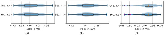
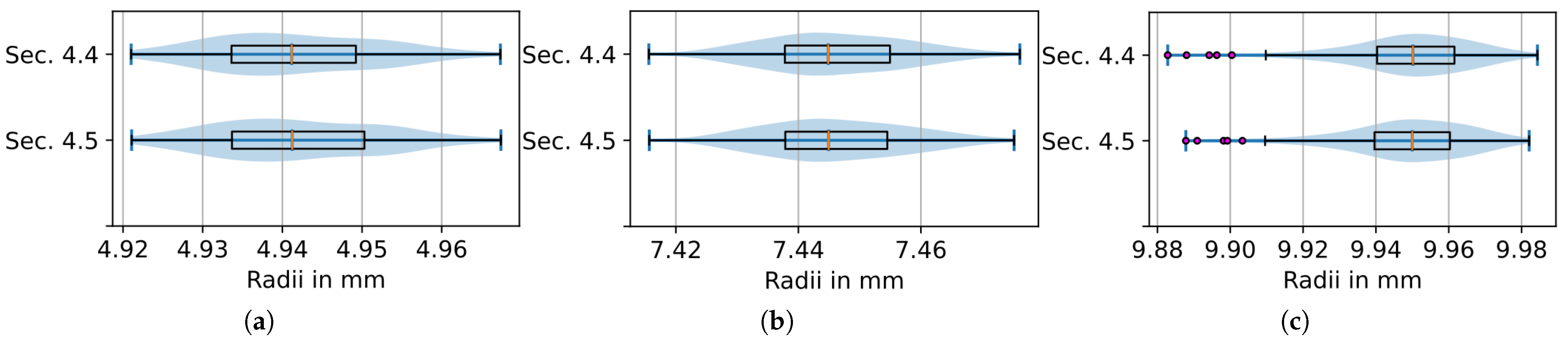
To evaluate the precision, the version with the radii introduced as unknowns was analyzed. The bundle adjustments were computed as free net adjustment with scale condition (Equation (43)). Due to a slight change in scale caused by the free net adjustment, the resulting circle centers and radii were scaled after the BA so that the scale bar distance fits to the reference value. Then, a statistical analysis of the scaled BA results for the 127 targets (excluding the 2 scale bar targets) was performed; see Figure 23. The combined violin and box plots show the range and the distribution of the estimated target radii for each of the three test fields. The estimated radii were within a range of 0.1 mm or less.

Further parameters for the evaluation of the precision are shown in

Table 13. Precision analysis of the radius determination in the BA for the different radii and models ($\Delta R_C=mean\left(R_{C,BA}\right)-R_{C,ref}$).

Model	${\mathit{R}}_{\mathit{C},\mathit{ref}}$ in mm	${\mathit{RMS}}_{\mathit{BA}}$ in px	$\mathit{mean}\left({\mathit{R}}_{\mathit{C},\mathit{BA}}\right)$ in mm	$\mathbf{\Delta }{\mathit{R}}_{\mathit{C}}$ in mm	$\mathbf{\Delta }{\mathit{R}}_{\mathit{C}}/{\mathit{R}}_{\mathit{C},\mathit{ref}}$ in %	$\mathit{mean}\left({\mathit{\sigma }}_{\mathit{RC},\mathit{BA}}\right)$ in mm	${\mathit{s}}_{{\mathit{R}}_{\mathit{C},\mathit{BA}}}$ in mm	${\mathit{s}}_{{\mathit{R}}_{\mathit{C},\mathit{BA}}}/{\mathit{R}}_{\mathit{C}}$ in %
Section 4.4	5.0	0.050	4.942	−0.058	−1.2	0.0029	0.011	0.21
Section 4.5	5.0	0.077	4.942	−0.058	−1.2	0.0010	0.011	0.21
Section 4.4	7.5	0.048	7.446	−0.054	−0.72	0.0029	0.012	0.16
Section 4.5	7.5	0.076	7.446	−0.054	−0.72	0.0010	0.012	0.16
Section 4.4	10.0	0.037	9.948	−0.052	−0.52	0.0032	0.019	0.19
Section 4.5	10.0	0.075	9.948	−0.052	−0.52	0.0009	0.018	0.18

: the mean estimated target radius of the BA $mean\left(R_{C,BA}\right)$, and the mean resulting standard deviation of the radii from the stochastic model of the BA. Furthermore, the scattering of the 127 estimated target radii was expressed by their empirical standard deviation $s_{R_{C,BA}}$, which can be considered as a more representative precision quantity. The relative precision $s_{R_C}/R_C$ ranged from 0.0011 to 0.0021 depending on the target size: the larger the radii, the smaller (better) the relative precision. The results show an underestimation of the radii of 0.05 to 0.06 mm. The relative errors $\Delta R_C/R_{C,ref}$ were negative and were smaller with increasing radius.

6.2. Accuracy Analysis

The accuracy was evaluated comparing the scale bar distance of the BA results with fixed radii (that defines the scale) and the reference scale bar distance. Note that only six constraints of the free net adjustment were applied in this case:

$$\begin{array}{c}\hfill \sum _{i}d{\overrightarrow{X}}_{C,i}=\overrightarrow{0}\\ \hfill \sum _i{\overrightarrow{X}}_{C,i}\times d{\overrightarrow{X}}_{C,i}=\overrightarrow{0}\end{array}$$

(44)

Table 14. Accuracy analysis of the scale definition by different radii and models.

Model	${\mathit{R}}_{\mathit{C},\mathit{ref}}$ in mm	${\mathit{RMS}}_{\mathit{BA}}$ in px	${\mathit{d}}_{\mathit{scalebar},\mathit{estimated}}$ in mm	${\mathit{d}}_{\mathit{scalebar},\mathit{target}}$ in mm	Difference in mm	Relative Error in %
Section 4.4	5.0	0.050	748.968	740.289	−8.679	−1.2
Section 4.5	5.0	0.082	748.920	740.289	−8.631	−1.2
Section 4.4	7.5	0.048	745.621	740.289	−5.332	−0.72
Section 4.5	7.5	0.081	745.600	740.289	−5.311	−0.72
Section 4.4	10.0	0.037	744.124	740.289	−3.835	−0.52
Section 4.5	10.0	0.088	744.159	740.289	−3.870	−0.52

reveals the results of the comparison of the distances of the scale bar for the three different radii and the two different models (Section 4.4 and Section 4.5). The deviations in the scale bar target distance ranged from 3.9 mm to 8.7 mm. These correspond to relative errors in the range of 0.5% to 1.2%, depending on the target radii: the larger the target radii, the smaller the relative and absolute scale error.

The experiment showed that this method for scale definition is not suitable for high-accuracy measurements, but can be used for applications with lower accuracy requirements. Note that there is a limited printing accuracy of the targets, which also influences the accuracy of the scale definition by radii and which may also affect the results.

7. Conclusions and Outlook

This article shows different correction methods for the eccentricity effect of circular targets in perspective projections. These eccentricity effects cause image coordinate measurement errors, which may be, by up to two orders of magnitude, larger than the actual image coordinate measurement precision using subpixel-accuracy operators. Five different methods were developed, two of which are applied in the image space in combination with the standard pinhole model, and the others work through a model adaption. The choice of the most suitable method depends on the computational effort, the target design and if circle normals can be obtained.

Table 15. Comparison of methods.

Method	Advantages	Disadvantages
Ecc. corr. in image space (Section 4.1, Equation (8))	Small computational effort in BA Ecc. completely corrected Usage of standard pinhole model	Target radii and normals must be given
Approximate ecc. corr. in image space (Section 4.1, Equation (13))	Small computational effort in BA Ecc. partly corrected Usage of standard pinhole model	Target radii and normals must be given
Concentric circle target ecc. corr. in image space (Section 4.2, Equation (22))	Small computational effort in BA Ecc. quasi completely corrected Circle normal not required Usage of standard pinhole model	Image ellipse analysis of two rings Target radii ratio must be given Larger target size
Pinhole model for circles with fixed radii and normals (Section 4.3)	Small computational effort in BA Ecc. completely corrected	Target radii and normals must be given
Extended BA with pinhole model for circles (Section 4.4)	Ecc. completely corrected Target radii and normals are computed in BA	High computational effort in BA Initial target radii and normals required
BA with contour points (Section 4.5)	No eccentricity errors Target radii and normals are computed in BA	Very high computational effort in BA Initial target radii and normals required

provides decision-making assistance. The table shows six approaches. The first two belong together. In the second approach (colored in gray), the eccentricity calculation is replaced by an approximation. As the eccentricity error was only partly corrected by the approximate eccentricity correction method in the experiments, this method should be avoided.

The methods were first tested in an experiment with a planar test field of concentric circles, where the eccentricity reached values of up to 6 pixels for the inner rings and 23 pixels for the outer rings. For the analysis of all targets with different sizes, the eccentricity error was assessed by the RMS of the image residuals and similarity transformations of the circle centers. This error was strongly reduced by applying the corrections. When only equal-sized targets were used, it was difficult to demonstrate influences of the correction terms on the reprojection error and the adjusted circle centers due to correlations between target eccentricities and the interior, as well as exterior, orientation parameters. In addition, the methods were also applied to a non-planar test field with equal-sized targets, where the eccentricity effects could also be demonstrated and the corrections led to a significant reduction in remaining errors. The reprojection error was reduced by 22% and 48%, respectively. Average changes of up to 0.2 mm for the projection centers as well as the circle centers were shown.

The presented method of the extended bundle adjustment, as well as the bundle adjustment with the contour points, also offers the possibility of a scale definition by given target radii. This approach was tested in a further experiment, where relative scale definition accuracies of 0.5 to 1% were reached. This latter sub-method is thus only suitable for applications with lower accuracy requirements and depends on the accuracy of the target radii.

Future work could also investigate the inclusion of the image ellipse inclination angle as observation in the extended bundle adjustment. Additionally, further investigations could be conducted to analyze the accuracy of the scale definition with non-planar test fields. Another interesting point could be the analysis of the influence of the eccentricity to the lens distortion parameters.

References

- Liebold, F.; Maas, H.G. Eccentricity Correction Methods for Circular Targets in Perspective Projection. Int. Arch. Photogramm. Remote Sens. Spat. Inf. Sci. 2024, 48, 65–72. [Google Scholar] [CrossRef] [Scilit]
- Luhmann, T.; Fraser, C.; Maas, H.G. Sensor modelling and camera calibration for close-range photogrammetry. ISPRS J. Photogramm. Remote Sens. 2016, 115, 37–46. [Google Scholar] [CrossRef] [Scilit]
- Lenz, R.; Fritsch, D. On the Accuracy of Videometry. Int. Arch. Photogramm. Remote Sens. Spat. Inf. Sci. 1988, 27-B5, 335–345. [Google Scholar]
- Andresen, K. Calculation of analytical elements in space using a contour algorithm. In Close-Range Photogrammetry Meets Machine Vision; International Society for Optics and Photonics: Bellingham, WA, USA, 1990; Volume 1395, p. 139533. [Google Scholar] [CrossRef] [Scilit]
- Dold, J. Influence of Target Size on the Results of Photogrammetric Bundle Adjustment. Int. Arch. Photogramm. Remote Sens. Spat. Inf. Sci. 1996, 31, 119–123. [Google Scholar]
- Heikkilä, J.; Silvén, O. A four-step camera calibration procedure with implicit image correction. In Proceedings of the IEEE Computer Society Conference on Computer Vision and Pattern Recognition, San Juan, PR, USA, 17–19 June 1997; pp. 1106–1112. [Google Scholar] [CrossRef] [Scilit]
- Ahn, S.J.; Warnecke, H.J.; Kotowski, R. Systematic geometric image measurement errors of circular object targets: Mathematical formulation and correction. Photogramm. Rec. 1999, 16, 485–502. [Google Scholar] [CrossRef] [Scilit]
- Otepka, J.; Fraser, C. Accuracy Enhancement of Vision Metrology Through Automatic Target Plane Determination. Int. Arch. Photogramm. Remote Sens. Spat. Inf. Sci. 2004, 35-B5, 873–879. [Google Scholar]
- Wrobel, B.P. Kreismarken in perspektiver Abbildung–im Bild und im Bündelblock. PFG-J. Photogramm. Remote Sens. Geoinf. Sci. 2012, 16, 221–236. [Google Scholar] [CrossRef] [Scilit]
- He, D.; Liu, X.; Yin, Y.; Li, A.; Peng, X. Correction of circular center deviation in perspective projection. In Proceedings of the Applications of Digital Image Processing XXXV; Tescher, A.G., Ed.; International Society for Optics and Photonics, SPIE: Bellingham, WA, USA, 2012; Volume 8499, pp. 625–631. [Google Scholar] [CrossRef] [Scilit]
- Kim, J.S.; Kim, H.W.; Kweon, I. A camera calibration method using concentric circles for vision applications. In Proceedings of the ACCV2002: The 5th Asian Conference on Computer Vision, Melbourne, Australia, 23–25 January 2002; pp. 23–25. [Google Scholar]
- Luhmann, T. Eccentricity in images of circular and spherical targets and its impact on spatial intersection. Photogramm. Rec. 2014, 29, 417–433. [Google Scholar] [CrossRef] [Scilit]
- Matsuoka, R.; Maruyama, S. Eccentricity on an image caused by projection of a circle and a sphere. ISPRS Ann. Photogramm. Remote Sens. Spat. Inf. Sci. 2016, 3, 19–26. [Google Scholar] [CrossRef] [Scilit]
- Yang, X.; Fang, S. Eccentricity error compensation for geometric camera calibration based on circular features. Meas. Sci. Technol. 2014, 25, 025007. [Google Scholar] [CrossRef] [Scilit]
- Shen, Y.; Zhang, X.; Cheng, W.; Zhu, L. Quasi-eccentricity error modeling and compensation in vision metrology. Meas. Sci. Technol. 2018, 29, 045006. [Google Scholar] [CrossRef] [Scilit]
- Bethmann, F.; Luhmann, T. Least-squares matching with advanced geometric transformation models. Int. Arch. Photogramm. Remote Sens. Spat. Inf. Sci. 2010, 38, 86–91. [Google Scholar]
- Brown, D.C. Close-Range Camera Calibration. Photogramm. Eng. 1971, 37, 855–866. [Google Scholar]
- El-Hakim, S.F. Real-Time Image Metrology with CCD Cameras. Photogramm. Eng. Remote Sens. 1986, 52, 1757–1766. [Google Scholar]
- Luhmann, T. Ein Verfahren zur rotationsinvarianten Punktbestimmung. Bildmess. Luftbildwes. 1986, 4, 147–154. [Google Scholar]
- Luhmann, T.; Robson, S.; Kyle, S.; Boehm, J. Close-Range Photogrammetry and 3D Imaging; De Gruyter: Berlin, Germany; Boston, MA, USA, 2020. [Google Scholar] [CrossRef] [Scilit]
- Zhou, G. Accurate Determination of Ellipse Centers in Digital Imagery. ACSM-ASPRS Annu. Conv. 1986, 4, 256–264. [Google Scholar]
- DIN 18709-4-2010; Concepts, Abbreviations and Symbols in Geodesy—Part 4: Adjustment of Observations and Statistics. DIN Deutsches Institut für Normung e.V.: Berlin, Germany, 2010. [CrossRef] [Scilit]
- Godding, R. Photogrammetric method for the investigation and calibration of high-resolution camera systems. In Proceedings of the SPIE 1987, Recording Systems: High-Resolution Cameras and Recording Devices and Laser Scanning and Recording Systems, Munich, Germany, 21–25 June 1993. [Google Scholar] [CrossRef] [Scilit]
- Liebold, F.; Maas, H.G. Spherical target eccentricity correction in photogrammetric applications. ISPRS J. Photogramm. Remote Sens. 2026, 231, 761–777. [Google Scholar] [CrossRef] [Scilit]
Disclaimer/Publisher’s Note: The statements, opinions and data contained in all publications are solely those of the individual author(s) and contributor(s) and not of MDPI and/or the editor(s). MDPI and/or the editor(s) disclaim responsibility for any injury to people or property resulting from any ideas, methods, instructions or products referred to in the content. |
© 2026 by the authors. Licensee MDPI, Basel, Switzerland. This article is an open access article distributed under the terms and conditions of the Creative Commons Attribution (CC BY) license.