Ethanol Concentration Sensing Using a 3D-Printed Microwave Cavity Resonator

Abstract

This work presents microwave sensing of ethanol concentration in ethanol–water mixtures using a low-cost 3D-printed cavity resonator. The objective is to realize a customizable liquid sensor that combines high measurement accuracy with inexpensive, in-house fabrication. The cylindrical cavity is fabricated from polylactic acid using fused deposition modeling and metallized on its inner surface with copper tape. The resonator operates in the TM₀₁₀ mode with a resonant frequency of 3 GHz. A standard 1.5 mL centrifuge tube is used as a modular sample holder and inserted through a circular opening in the top endcap of the cavity. The quality factor of the air-filled cavity is 200, which decreases to 37.3 when the cavity is loaded with deionized water. As an application example, ethanol concentrations in ethanol–water mixtures are determined using both the resonant frequency and the peak magnitude of the transmission coefficient (|S₂₁|). For ethanol concentrations between 20% and 100%, the concentration can be accurately extracted from the resonant frequency alone: a quartic calibration curve yields a coefficient of determination $R^2=0.9992$, an average sensitivity of approximately 8.4 MHz/% ethanol, and a mean absolute error of about 0.58% on the calibration set. In addition, a cubic calibration based on the peak $\mid S_{21}\mid$ over the 0–90% concentration range achieves a mean absolute error of approximately 0.52% on the calibration set and about 0.55% on an independent validation set covering 5–85% ethanol. Comparison with conventionally machined metal cavities shows that the proposed 3D-printed cavity achieves a high Q-factor at significantly lower cost and can be fabricated in-house using a standard 3D printer. These results demonstrate metrologically relevant performance in terms of low error and high sensitivity using a low-cost and easily replicable platform for microwave liquid sensing in biomedical and chemical engineering applications.

1. Introduction

The microwave cavity resonator is a mature and widely adopted technology for non-destructive characterization of dielectric materials, with a vast and growing body of research demonstrating its utility across diverse scientific and industrial domains. Its ability to perform highly sensitive measurements stems from the high-quality factor (Q-factor) of the resonant structure, which enables precise detection of resonant frequency shifts that correlate directly with the material’s complex dielectric constant (${\epsilon }_r^{*}={{\epsilon }_r^{\prime }-j\epsilon }_r^{″}$). For the characterization of liquids, various microwave sensor designs have been successfully implemented, including planar resonant structures to discriminate between ethanol and methanol with high precision [1] and engineered cylindrical cavities to measure trace concentration differences in aqueous solutions [2], detect contaminants in lubricating oil [3], and characterize extremely low-loss coolants for data centers [4]. Innovations in resonator geometry, such as rectangular cavities with top-side insertion holes, have simplified sample handling [5], while slotted cylindrical resonators have enabled wireless, chipless liquid-level sensing [6]. These methods are consistently supported by rigorous analytical techniques that enhance accuracy in permittivity extraction [7].

Beyond liquids, microwave resonators are routinely applied to solid, granular, and engineered materials. They have proven highly effective for ultrasensitive moisture content characterization in wood for applications like forest fire prevention [8] and for ensuring uniform field distribution during moisture measurements in granular substances such as grains and powders [9]. In the electronics industry, specialized TM₀₁₀ mode resonators are essential for the accurate extraction of dielectric constant (Dk) and dissipation factor (Df) in printed circuit board (PCB) materials, with studies focusing on both analytical modeling [10] and the optimization of probe configurations to ensure measurement fidelity [11]. The versatility of this technology is further highlighted in specialized applications, such as real-time steam wetness monitoring in turbines to prevent blade damage [12] and the characterization of small, high-loss biological tissues at millimeter-wave frequencies [13].

Complementing these diverse applications are significant innovations in resonator design aimed at miniaturization, performance enhancement, and operation in new frequency regimes. To meet the demands of modern communication systems, partially metalized dielectric resonators have been developed to achieve a 30% size reduction without compromising the Q-factor [14]. At millimeter-wave frequencies, novel open-cavity designs have demonstrated remarkable Q-factors near 10,000 at 281 GHz [15], while re-entrant cavities fabricated via stereolithography (SLA) 3D printing and copper plating have achieved high sensitivity for liquid characterization at 60 GHz [16]. Application-specific designs are also prominent, such as RF cavities optimized for high-power klystrons [17]. The accuracy of these hardware implementations is continually reinforced by robust computational methodologies that correct for systemic errors from insertion holes [18] and sample tilt [19], improve computational speed [20,21], and provide advanced modeling for complex geometries and materials [22,23]. Furthermore, foundational techniques, like the cavity perturbation method, remain vital for accurately assessing a wide range of both low- and high-loss materials [24].

While the preceding review illustrates a field rich with high-performance and innovative solutions, a common thread linking many of these advanced systems is their reliance on conventional precision machining. This fabrication approach, though effective, is often costly and time-consuming, creating a significant barrier to the rapid prototyping of custom sensors and limiting their deployment in educational or resource-constrained environments. Although 3D printing enables rapid prototyping and the fabrication of complex geometries, the realization of high-Q cavity resonators requires additional metal plating and surface treatment. Metal additive manufacturing offers an alternative by directly producing conductive cavity structures; however, metal 3D printing involves high capital costs, requires skilled operators for printing and post-processing, and still demands surface finishing to achieve high Q-factors. Furthermore, in resource-limited environments, the deployment of microwave sensors—particularly those operating at millimeter-wave and sub-terahertz frequencies—is constrained by the high cost of high-frequency vector network analyzers. This highlights a critical need for accessible, cost-effective, and easily customizable fabrication approaches that broaden access to sensor development.

In parallel with these high-performance designs, there is increasing interest in low-cost microwave metrology platforms that leverage commercial 3D printers, simple metallization, and low-cost instrumentation to broaden access to dielectric characterization [25,26,27,28]. Several recent studies have explored 3D-printed resonators and planar sensors for chemical and biomedical sensing, but most still rely on electroplating, vacuum deposition, or metal 3D printing to realize the conductive housing, which adds cost, requires specialized equipment, and limits deployment in resource-limited laboratories [29,30]. In contrast, adhesive copper tape offers an extremely inexpensive, rapid, and reworkable metallization method that can be applied to polymer-based cavities printed on standard fused deposition modeling (FDM) printers, enabling in-house fabrication, straightforward geometric customization, and compatibility with low-cost vector network analyzers for educational, industrial, and biomedical settings where conventional precision machining or metal 3D printing may be impractical [31,32].

To address this critical gap, this study presents a low-cost, rapidly prototyped cylindrical cavity resonator for the dielectric characterization of liquid mixtures. The cavity body is fabricated using FDM 3D printing with polylactic acid filament, and its inner surfaces are made conductive by applying adhesive copper tape. The proposed cavity resonator is designed to operate in the TM₀₁₀ mode at 3 GHz under air-filled conditions, and its suitability for liquid composition analysis is demonstrated by measuring systematic changes in both the resonant frequency and S₂₁ magnitude of the resonant peak (|S₂₁|_peak) as functions of ethanol concentration in ethanol–water mixtures contained in standard 1.5 mL centrifuge tubes. Measurements were carried out using a low-cost vector network analyzer, supporting the cost-effective nature of the proposed system. This approach provides a practical and economical route to highly customizable microwave sensors for chemical engineering and biomedical engineering applications, as well as for educational and research purposes.

The remainder of this paper is organized as follows. Section 2 describes the design and fabrication of the proposed cavity resonator, along with the experimental setup and preparation of the liquid under test (LUT). Section 3 analyzes the frequency-shift behavior with respect to the dielectric constant. Section 4 concludes the paper.

2. Materials and Methods

2.1. Resonator Design and Simulation

The cylindrical cavity resonator is designed to operate in the fundamental TM₀₁₀ mode, for which the resonant frequency $f_0$ is primarily determined by the cavity inner radius R. For an ideal unloaded cavity, the theoretical relationship is given by [7] with

$$f_0={\displaystyle \frac{p_{01}c}{2\pi R}}$$

(1)

where $p_{01}$ is the first root of the zeroth-order Bessel function with $p_{01}$ ≈ 2.405, and $c$ is the speed of light. For practical implementation, this relationship is simplified into a design equation that relates the radius R in centimeters to the frequency in gigahertz:

$$R\left(cm\right)={\displaystyle \frac{11.5}{f_0\left(\mathrm{GHz}\right)}}$$

(2)

The operating frequency was set to approximately 3 GHz in the TM₀₁₀ mode to balance cavity size, dielectric response, and instrumentation constraints. At this frequency, the required cavity radius yields a compact structure that still accommodates a standard 1.5 mL centrifuge tube and maintains sufficient wall thickness for robust FDM 3D printing and copper-tape metallization. In addition, ethanol–water mixtures exhibit strong, monotonic changes in complex permittivity in the few gigahertz range without excessive dielectric loss, enabling large, well-resolved resonance frequency shifts with concentration while preserving a usable Q-factor. Finally, 3 GHz lies within the bandwidth of low-cost vector network analyzers, allowing complete characterization of the sensor using inexpensive instrumentation, which is consistent with the low-cost microwave metrology focus of this work.

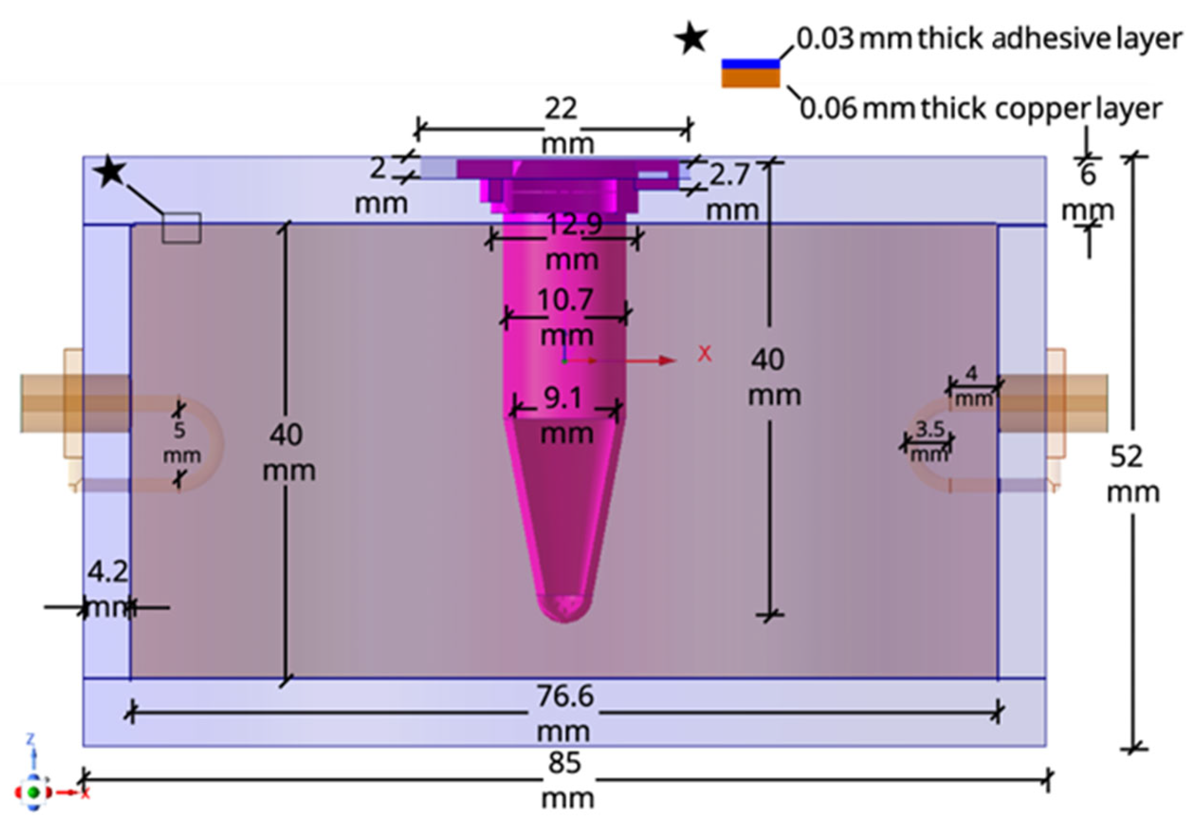
For a target resonant frequency of 3 GHz, the inner radius of the cavity is initially calculated to be 3.83 cm using Equation (2). To introduce the sample, a circular insertion hole with a diameter of 10.7 mm is incorporated into the cavity top endcap and centered on the axis to coincide with the electric field maximum. For a cylindrical cavity resonator operating in the TM₀₁₀ mode, the resonant frequency is theoretically independent of the cavity height h. However, the unloaded Q-factor $Q_u$ is directly influenced by the cavity height, exhibiting an inverse proportionality with $Q_u\propto {\displaystyle \frac{1}{h}}$ [33,34]. The complete geometry was modeled and optimized using a full-wave numerical simulation tool (Ansys HFSS) to achieve the required response prior to fabrication.

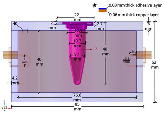
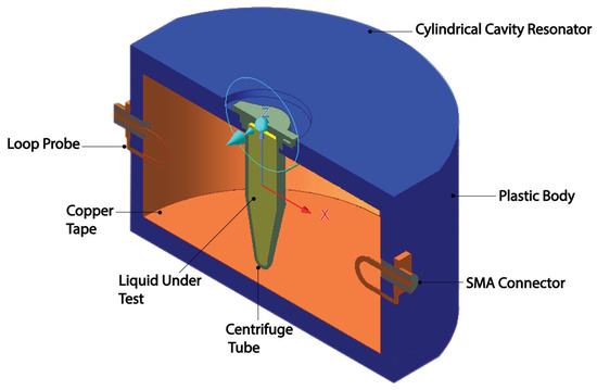
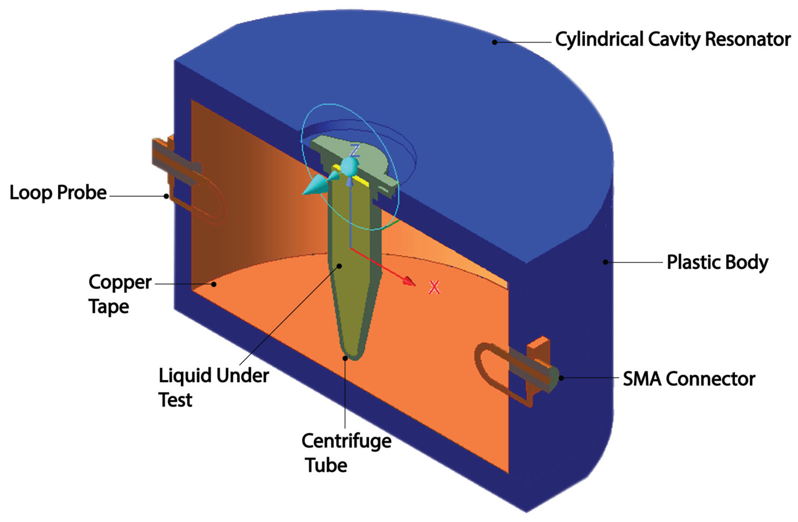
The simulation model viewed with a cross-sectional cut plane with dimensions is shown in Figure 1. The cross-sectional, isometric view of the model can be seen in Figure 2. Except for the LUT, all material parameters of the model are provided in the material library of HFSS. The cavity top endcap is designed to incorporate the sample holder. The centrifuge tube is inserted into the cavity through the insertion hole, while its cap, which has a larger diameter than the tube body, rests on an integrated support on the top surface of the endcap. This configuration securely holds the tube in an upright position, aligned with the cylindrical cavity axis. Two SMA ports are mounted at diametrically opposite locations on the outer wall of the cavity to enable measurement of S21. Magnetic loop probes are used for coupling. Each probe is formed by extending the inner conductor of an SMA connector into a loop and soldering it to the connector’s outer conductor. The loop is centered at the midpoint of the cavity height.

Figure 1. Cross-sectional view of the proposed cylindrical cavity resonator with dimensions. The star indicates the close-up detail of the copper tape used to metallize the interior surface of the cavity.

Figure 2. Cross-sectional, isometric view of the 3D-printed cylindrical cavity resonator.

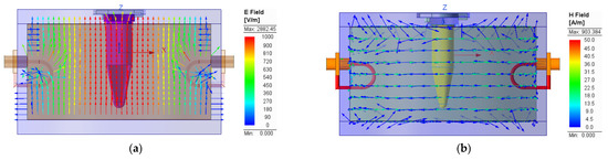
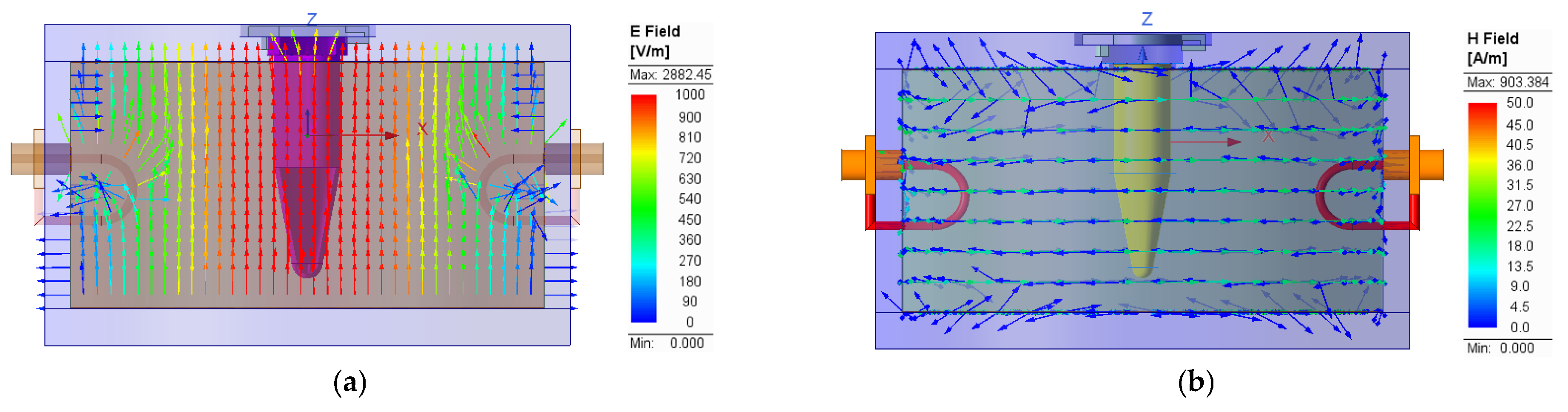
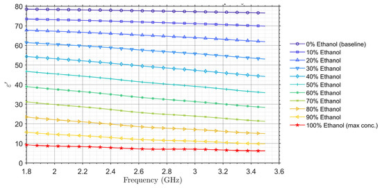
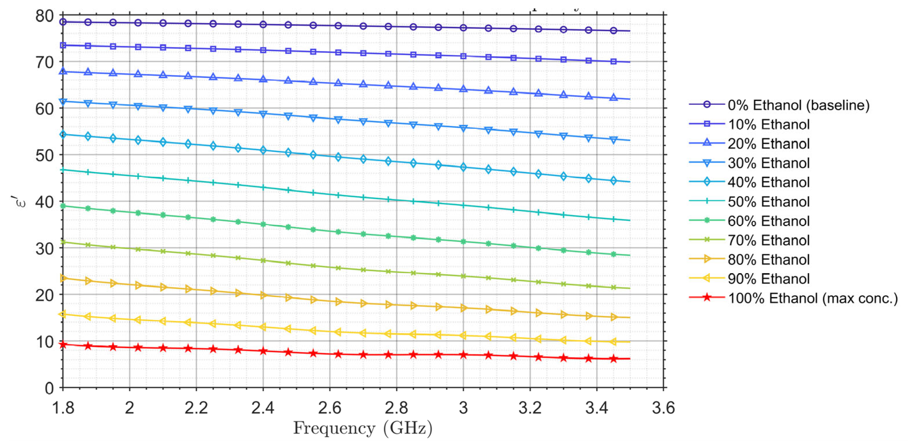
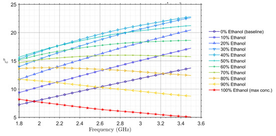
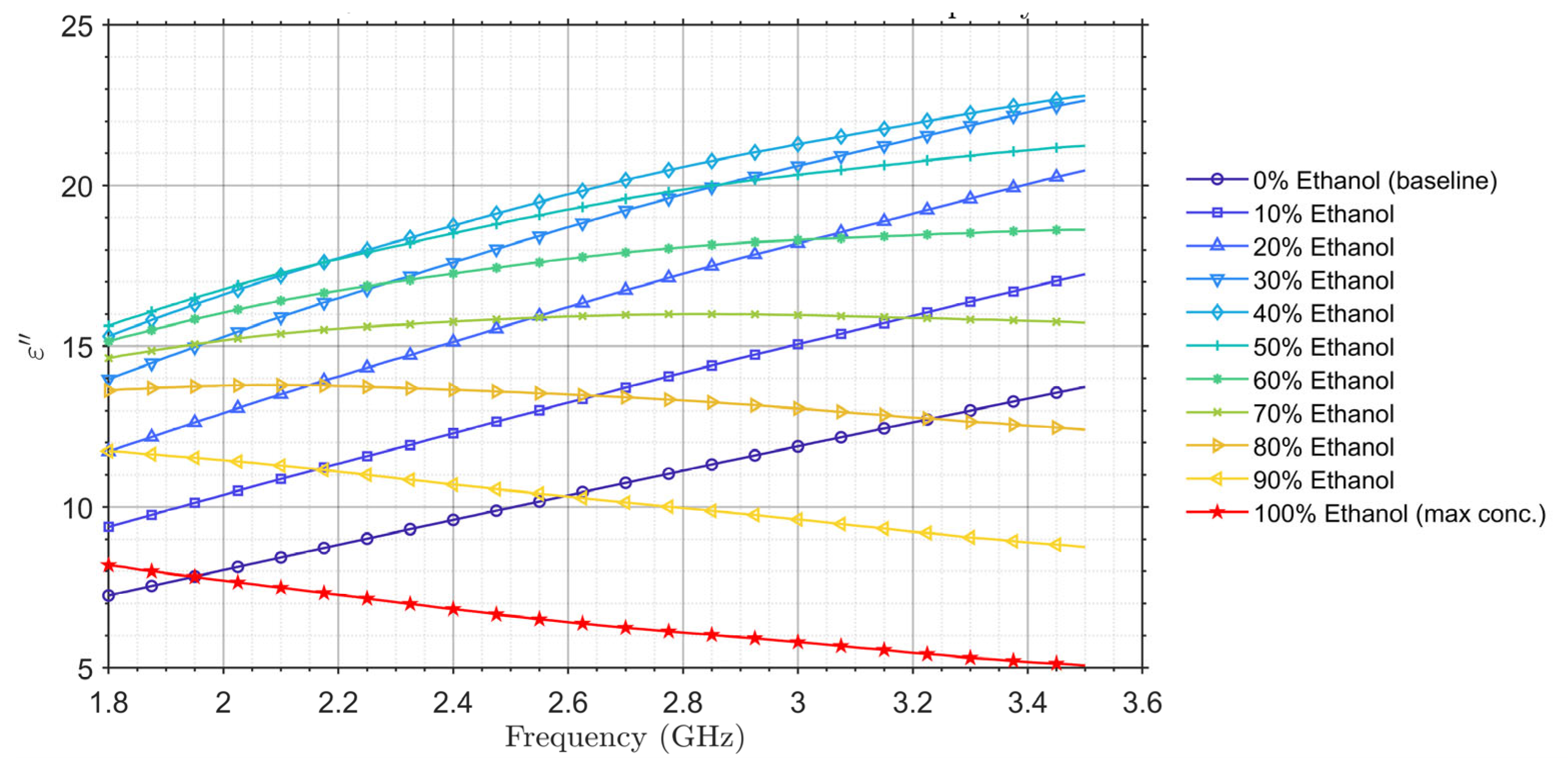
Figure 3a,b shows the simulated electric field distributions for the TM₀₁₀ mode with an empty centrifuge tube at the resonant frequency of 3 GHz. To evaluate the cavity resonator’s potential for sensing ethanol concentration in ethanol–water mixtures, samples with various ethanol concentrations were prepared and characterized using a commercial dielectric measurement probe. Details about the measurement system and setup can be found in [35]. The frequency-dependent dielectric properties obtained from the measurements are presented in Figure 4 and Figure 5.

Figure 3. Simulation results of: (a) E-field distribution; (b) H-field distribution in the cross-sectional plane of the proposed cavity resonator. The arrows indicate the instantaneous electric and magnetic field directions at a particular phase of the signal.

Figure 4. Measured dielectric constant of the ethanol–DI water mixtures using the commercial dielectric measurement probe.

Figure 5. Measured dielectric loss factor of ethanol–DI water mixtures using the commercial dielectric measurement probe.

In Figure 4, measured dielectric properties of ethanol–deionized (DI) water mixtures with various ethanol concentrations are presented across the 1.8–3.5 GHz frequency range. The results reveal a clear, monotonic decrease in the real part of the complex relative permittivity (${\epsilon }_r^{\prime }$) with increasing ethanol concentration, starting from approximately 78 for pure DI water and dropping to around 10 for pure ethanol at 1.8 GHz. This trend is also presented at other frequencies throughout the frequency range of interest. These results are consistent with established literature values and demonstrate the effectiveness of dielectric spectroscopy for quantifying ethanol concentration in the mixtures [36,37,38,39].

According to Figure 5, the dielectric loss factor (${\epsilon }_r^{″}$) of ethanol–DI water mixtures was thoroughly characterized across ethanol concentrations ranging from 0% (pure DI water) to 100% (pure ethanol) over the 1.8–3.5 GHz frequency range. As the concentration of ethanol changes, the complex hydrogen-bonding network and molecular relaxation processes are altered, leading to a frequency-dependent variation in the mixture’s dielectric loss factor [40,41]. The measured results reveal pronounced dielectric dispersion, attributed to the superposition of the distinct molecular relaxation mechanisms of water and ethanol. For pure DI water, the dielectric loss factor exhibits a low but sharply increasing trend with frequency, consistent with the low-frequency tail of water’s primary Debye relaxation peak. In contrast, pure ethanol displays a much flatter response, resulting in a decreasing trend of dielectric loss factor throughout the 1.8–3.5 GHz frequency range. This opposing behavior produces a distinct ${\epsilon }_r^{″}$ crossover around an ethanol concentration of 40–50%. From the dielectric constant and the dielectric loss factor, the loss tangent $\left(\tan \delta \right)$ can be derived with

$$\tan \delta ={\displaystyle \frac{{\epsilon }_r^{″}}{{\epsilon }_r^{\prime }}}$$

(3)

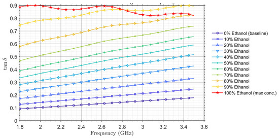
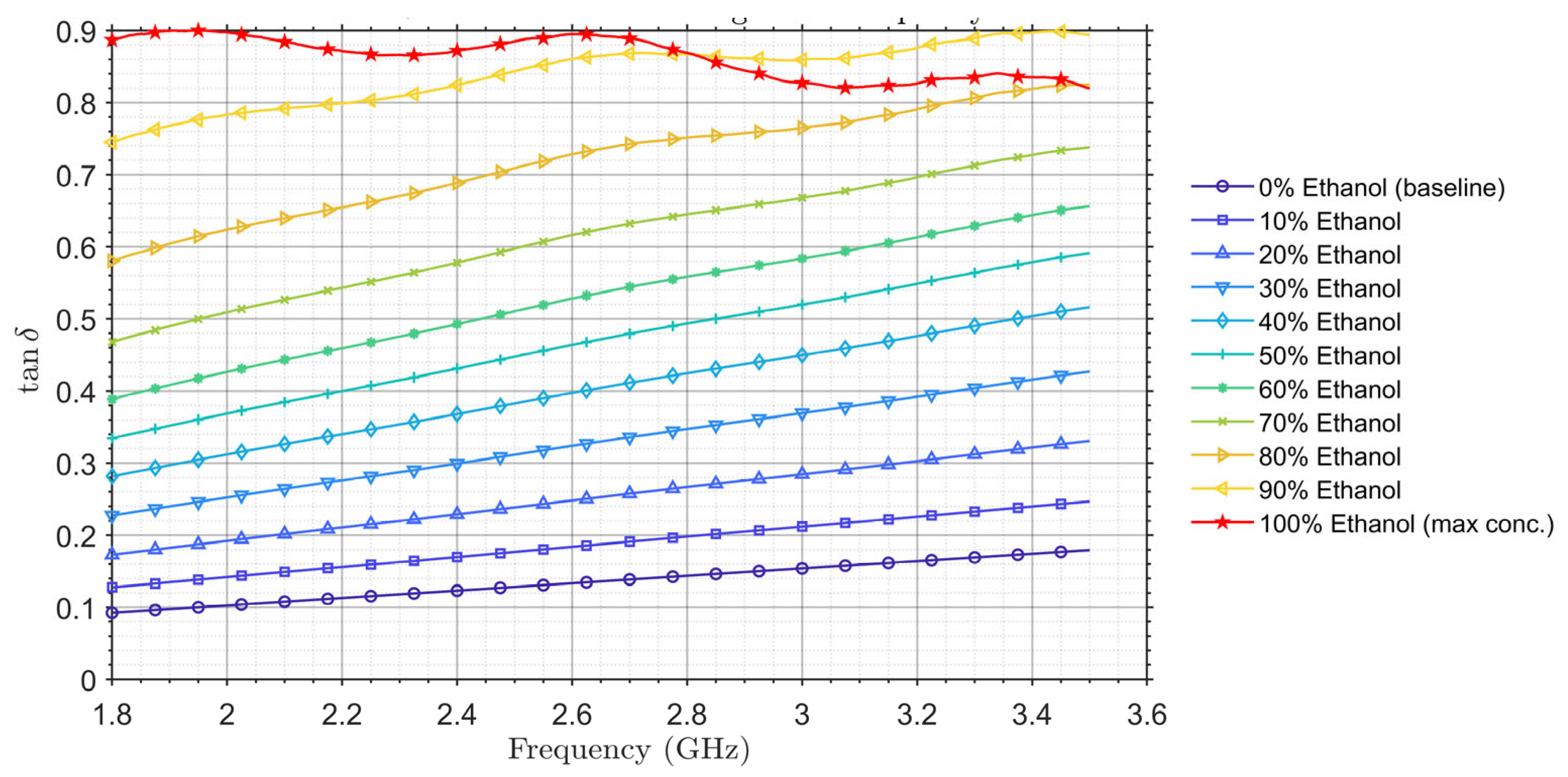
In Figure 6, $\tan \delta$ derived from the measured ${\epsilon }_r^{\prime }$ and ${\epsilon }_r^{″}$ of the mixtures is shown across the 1.8–3.5 GHz frequency range. Except for 100% ethanol, $\tan \delta$ exhibits a clear increasing trend toward higher ethanol concentration of the mixture and higher frequency. This trend is primarily driven by the significant reduction in the mixture’s relative permittivity (${\epsilon }_r^{\prime }$) as ethanol content increases, a factor that dominates the ratio even as the loss factor (${\epsilon }_r^{″}$) shows a more complex, non-monotonic crossover behavior.

Figure 6. Measured loss tangent of the ethanol–DI water mixtures from the commercial dielectric measurement probe.

2.2. Fabrication of the Cavity Resonator

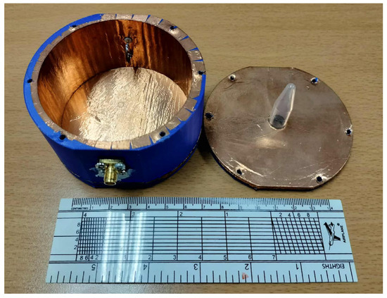
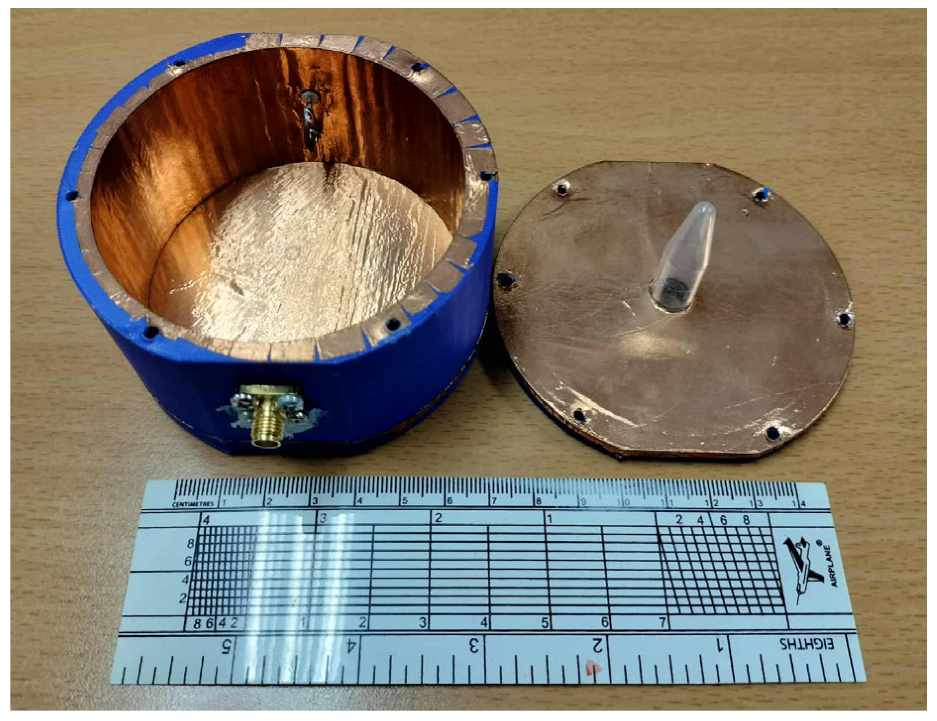
The cavity resonator structure was fabricated using an FDM 3D printer with polylactic acid (PLA) filament according to the design in Figure 3. To achieve the desired conductive cavity walls and endcaps, the inner surfaces of the 3D-printed PLA cavity were carefully lined with adhesive copper tape. The upper and lower caps of the resonator and the main body are joined using M5 screws. A photograph of the fabricated cavity resonator can be seen in Figure 7.

Figure 7. A photograph of the fabricated 3D-printed cylindrical cavity resonator.

2.3. Measurement Setup

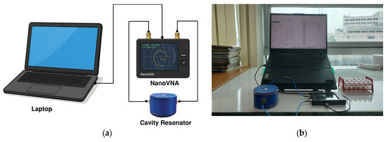
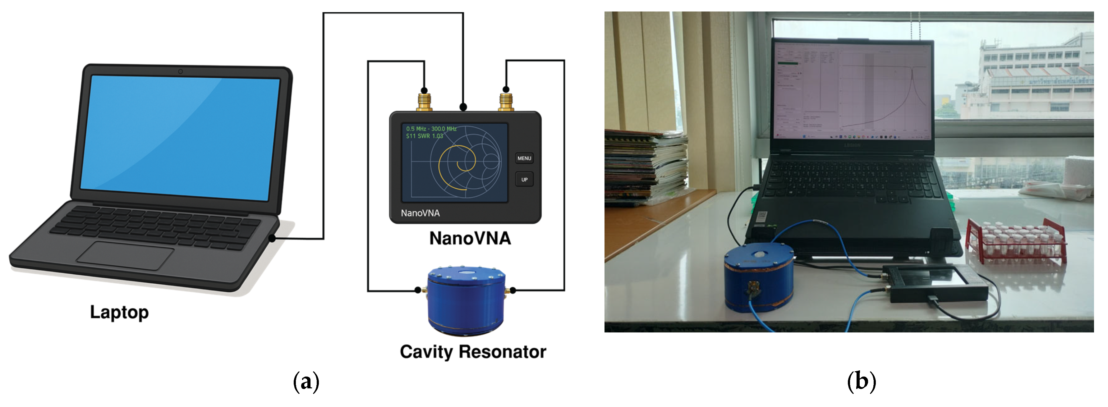
The fabricated cavity resonator was connected to a low-cost vector network analyzer (NanoVNA, manufactured by AURSINC, Shenzhen, China, 50 kHz–6.3 GHz [42]) via RF cables to measure the magnitude of the forward transmission coefficient (|S₂₁|). The NanoVNA was calibrated using a standard short–open–load–through (SOLT) procedure over the frequency range of 1.8–3.5 GHz, with the reference plane set at the end of the measurement cables, using a 501-point sweep, and then connected to a laptop to view and save the measurement results. The instrument covers 50 kHz–6.3 GHz and provides a system dynamic range greater than 70 dB below 3 GHz (IF bandwidth = 1800 Hz), with an S-parameter noise floor below −50 dB for $f<3$ GHz and frequency stability better than 0.5 ppm over the 0–50 °C range. Under the measurement conditions used here (1.8–3.5 GHz span, 501 points), the effective frequency step is approximately 3.4 MHz, which is sufficient to resolve the narrow resonance peaks around 3 GHz and the concentration-dependent shifts on the order of tens of megahertz. Each measurement point was averaged over three repeated measurements. All reported data points are directly connected by straight lines in the plots, and no smoothing was applied. For each LUT sample contained in a centrifuge tube, |S₂₁|was recorded. A connection diagram and a photograph of the complete measurement setup are shown in Figure 8a and Figure 8b, respectively.

Figure 8. Measurement setup of the fabricated cavity resonator: (a) block diagram; (b) photograph of the actual measurement system.

2.4. Sample Preparation

A series of ethanol–DI water mixtures with various ethanol concentrations was prepared as an LUT for the experiment. Analytical-grade ethanol (≥99.8% purity) and deionized water with a resistivity of 18.2 MΩ·cm were used for all mixtures. Starting with a stock solution of 100% ethanol, a total of 11 mixtures were prepared by dilution with DI water. Each liquid mixture was prepared in a final volume of 100 mL, with ethanol concentrations ranging from 100% down to 0% in 10% decrements. The precise volume of ethanol and DI water needed for each target concentration was determined using the dilution formula.

$$C_1{V}_1=C_2{V}_2$$

(4)

where

$C_1$ is the initial concentration of the ethanol used for dilution;

$V_1$ is the required volume of ethanol;

$C_2$ is the desired final concentration;

$V_2$ is the final desired volume.

Then the volume of the DI water needed is calculated as

$$V_{DI Water}=V_2-V_1$$

The volumes of ethanol and DI water were measured using volumetric glass pipettes (5−50 mL), ensuring volumetric accuracy better than ±0.5%. All mixtures were prepared and measured at $25\pm 0.5 °\mathrm{C}$, monitored with a calibrated thermometer, and each solution was vortexed for at least 30 s and gently inverted immediately before filling the tube to ensure mixture homogeneity and to avoid trapped air bubbles.

3. Results and Discussion

3.1. Measurement of Fabricated Cavity Resonator with an Empty Centrifuge Tube

This section presents a comprehensive analysis of the forward transmission coefficient (S₂₁), focusing on the resonance characteristics derived from both simulated and experimentally measured data for the resonant system containing an empty centrifuge tube. The primary objective is to determine the resonance frequency, peak S₂₁ magnitude, −3 dB bandwidth, and the Q-factor for each dataset, followed by a comparative assessment to validate the design from Figure 2.

|S₂₁| of the cavity resonator containing an empty centrifuge tube was examined over the 1.8–3.5 GHz frequency range by means of both simulation and measurement. Figure 9 compares the simulated and measured |S₂₁| responses of the cavity resonator with an empty centrifuge tube. The simulated and measured results show excellent agreement over the frequency range of interest, thereby validating the electromagnetic model of the cavity–tube configuration. The discrepancy at the low-frequency end resulted from the limited dynamic range of the NanoVNA. The extracted parameters from both simulation and measurement are summarized in Table 1. The resonant frequency (f₀) is the frequency at which |S₂₁|reaches its maximum value, while the −3 dB bandwidth (BW) was determined from the frequencies f₁ and f₂ at which |S₂₁|decreases by 3 dB from the peak. The Q-factor was then calculated using the relationship

$$Q={\displaystyle \frac{f_0}{BW}}$$

(5)

where

$Q$ is the quality factor;

$f_0$ is the resonant frequency;

$BW$ is the bandwidth with BW = f₂ − f_1.

Figure 9. Comparison of simulated and measured |S₂₁| response of the proposed cavity resonator with an empty centrifuge tube.

Figure 9. Comparison of simulated and measured |S₂₁| response of the proposed cavity resonator with an empty centrifuge tube.

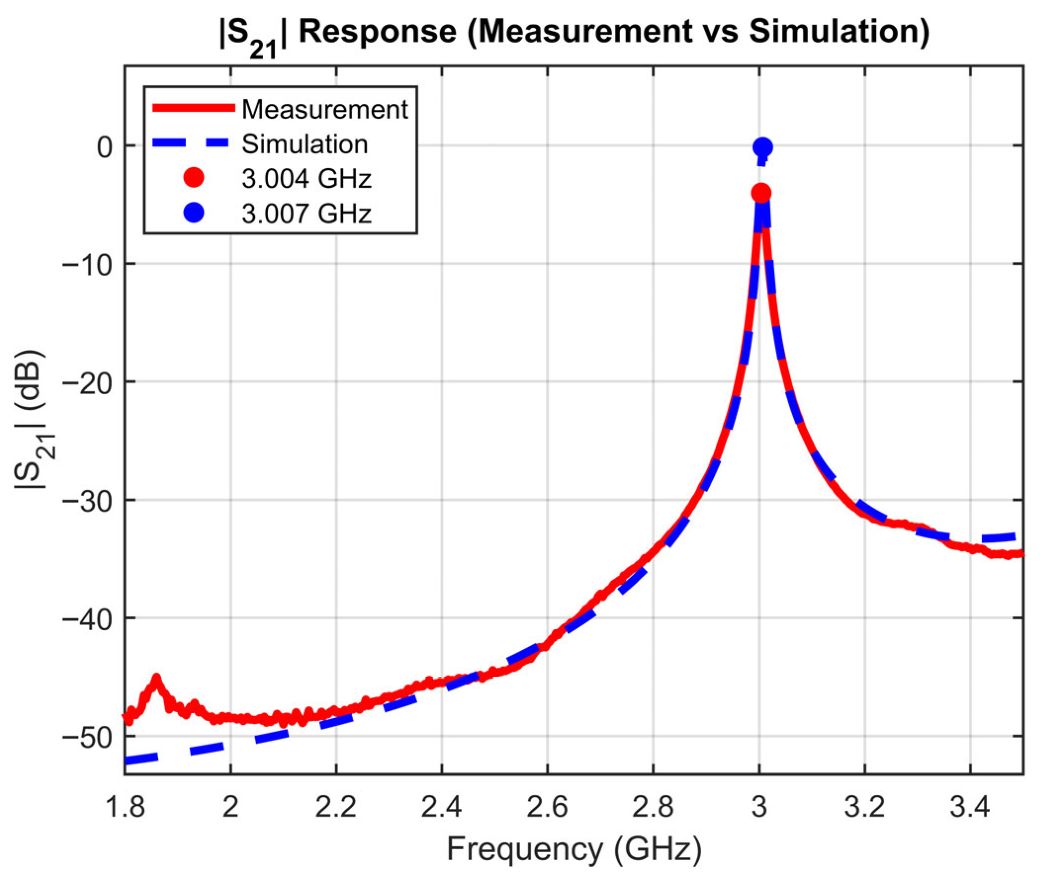
Table 1. Comparison of resonance characteristics from simulation and measurement data for the proposed cavity resonator with an empty centrifuge tube.

Parameter	Simulation	Measurement
Resonant frequency (f0)	3.007 GHz	3.004 GHz
Peak S21 Magnitude	−0.145 dB	−4.020 dB
Left −3 dB Frequency (f1)	2.999 GHz	2.997 GHz
Right −3 dB Frequency (f2)	3.011 GHz	3.012 GHz
3 dB Bandwidth (BW)	0.012 GHz	0.015 GHz
Q-factor	250.58	200.26

Table 1. Comparison of resonance characteristics from simulation and measurement data for the proposed cavity resonator with an empty centrifuge tube.

Parameter	Simulation	Measurement
Resonant frequency (f0)	3.007 GHz	3.004 GHz
Peak S21 Magnitude	−0.145 dB	−4.020 dB
Left −3 dB Frequency (f1)	2.999 GHz	2.997 GHz
Right −3 dB Frequency (f2)	3.011 GHz	3.012 GHz
3 dB Bandwidth (BW)	0.012 GHz	0.015 GHz
Q-factor	250.58	200.26

The peak |S₂₁| exhibits a significant discrepancy between simulation and measurement (−0.145 dB versus −4.020 dB), possibly due to practical loss mechanisms in the experimental setup, including conductor surface roughness, imperfect probe coupling, and finite contact resistance, none of which are accounted for in the idealized simulation model. An additional contributing factor is the limited frequency resolution of the NanoVNA, which may prevent accurate sampling of the narrow resonance peak. For the same reasons, the measured Q-factor of around 200 is lower compared to the simulated value of around 250. Nevertheless, the close agreement in spectral shape, bandwidth, and Q-factor between the simulated and measured|S₂₁| demonstrates that the fabricated cavity resonator is suitable for characterizing the LUT.

3.2. Simulation of |S₂₁| with Varying Ethanol Concentration

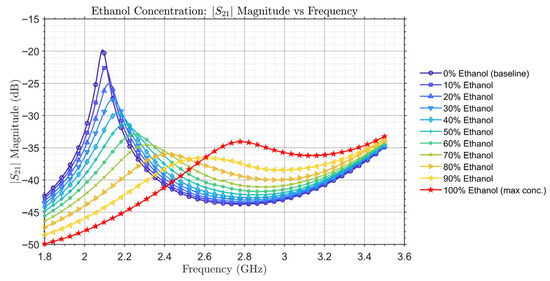
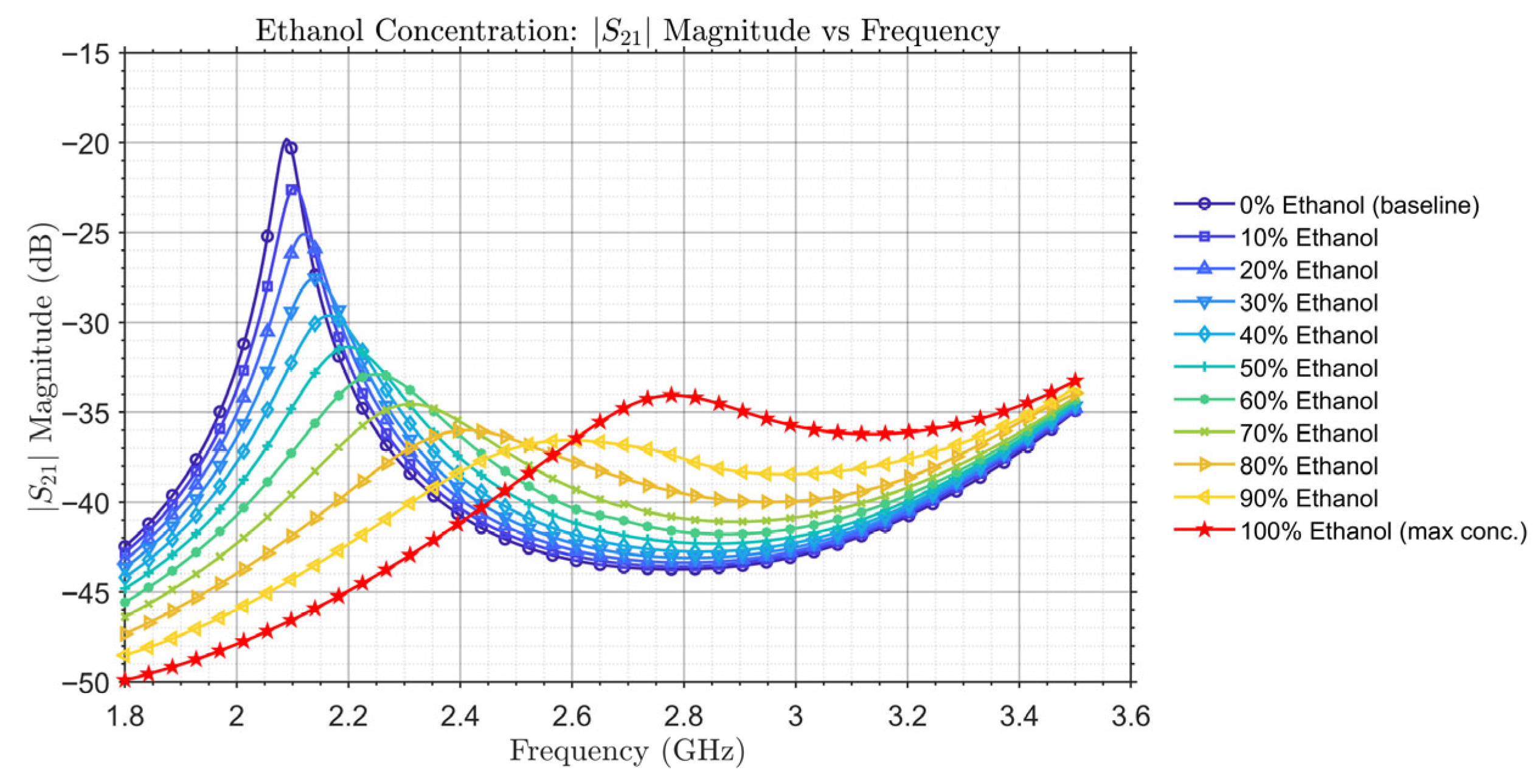
To investigate |S₂₁| characteristics with varying ethanol concentrations of the mixture contained in the centrifuge tube, the model from Figure 2 was simulated with the measured ${\epsilon }_r^{\prime }$ and ${\epsilon }_r^{″}$ of the mixtures from Figure 4 and Figure 5, respectively. The volume of the LUT contained in the centrifuge tube is 1.5 mL. Figure 10 depicts the simulated |S₂₁| with ethanol concentrations of the LUT from 0% to 100%. Due to different ${\epsilon }_r^{\prime }$ values of different ethanol concentrations, the resonant peaks show up at different frequency points within the 1.8 GHz to 3.5 GHz range. The resonant frequencies and |S₂₁|of the resonant peaks for all ethanol concentrations are summarized in Table 2.

Figure 10. Simulated |S₂₁| response for various ethanol concentrations of the LUT.

Table 2. Simulated resonant frequency and peak S₂₁ magnitude for various ethanol concentrations.

Ethanol Concentration (%)	Resonant Frequency (GHz)	Peak S21 Magnitude (dB)
0	2.089	−19.813
10	2.102	−22.475
20	2.119	−25.085
30	2.140	−27.534
40	2.166	−29.625
50	2.199	−31.376
60	2.250	−32.898
70	2.314	−34.545
80	2.412	−36.003
90	2.595	−36.552
100	2.782	−34.057

In Figure 10 and Table 2, a clear trend in resonant frequency is observed when varying the ethanol concentration. As the ethanol concentration increases from 0% to 100%, the resonant frequency of the cavity resonator consistently shifts towards higher frequencies. This behavior is physically consistent with the dielectric properties of the mixture, as ethanol possesses a significantly lower dielectric constant compared to DI water. Consequently, increasing the ethanol content effectively reduces ${\epsilon }_r^{\prime }$ of the mixture so that the resonant frequency is increased.

Except for pure ethanol, |S₂₁| decreases with increasing ethanol concentration, following the trend of $\tan \delta$ from Figure 6, which increases with increasing ethanol concentration. This suggests an increase in overall insertion loss and a reduction in the Q-factor as the ethanol content rises. Notably, a slight increase in|S₂₁| peak is observed for 100% ethanol compared to the 90% ethanol–DI water mixture. This non-monotonic behavior is likely attributed to the reversing trend of $\tan \delta$ in the case of pure ethanol observed in Figure 6. The distinct and systematic shift in the resonant frequency and the change of |S₂₁| peak demonstrate the resonator’s high sensitivity to varying ethanol content, laying the groundwork for its application as an ethanol concentration sensor.

3.3. Measurement of |S₂₁| with Varying Ethanol Concentration

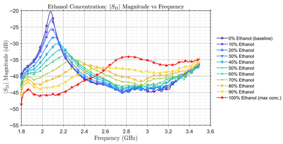
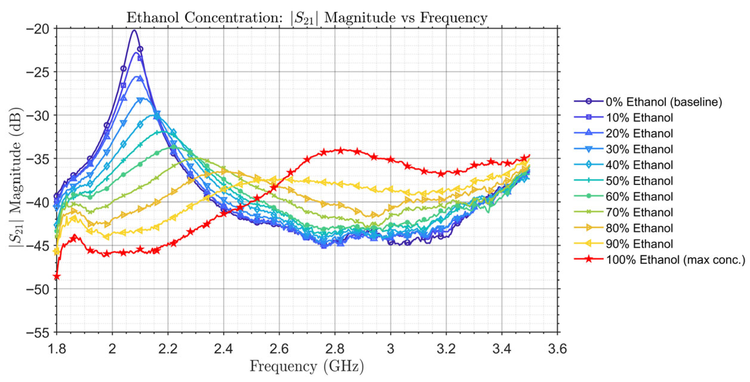
Following the simulation presented in Section 3.2, the resonator’s performance as an ethanol concentration sensor was experimentally evaluated with varying concentrations of ethanol in the LUT. Figure 11 illustrates the measured |S₂₁| across ethanol concentrations from 0% to 100%, with resonant peaks within the 1.8 GHz to 3.5 GHz range. The measured resonant frequencies and |S₂₁|of the resonant peaks for all ethanol concentrations are summarized in Table 3.

Figure 11. Measured |S₂₁| response for various ethanol concentrations of the LUT.

Table 3. Measured resonant frequency and peak S₂₁ magnitude for various ethanol concentrations.

Ethanol Concentration (%)	Resonant Frequency (GHz)	Peak S21 Magnitude (dB)
0	2.080	−20.213
10	2.084	−22.807
20	2.088	−25.585
30	2.112	−28.046
40	2.148	−30.016
50	2.176	−31.873
60	2.225	−33.653
70	2.304	−34.959
80	2.400	−36.476
90	2.584	−37.349
100	2.832	−33.953

The experimental results corroborate the trends observed in simulation results from Figure 10. As ethanol concentration increases, the resonant frequency consistently shifts to higher frequencies due to the mixture’s decreasing dielectric constant. Concurrently, |S₂₁|_peak decreases, indicating increasing losses in the SUT except for pure ethanol. At low transmission magnitude levels (approximately −40 to −45 dB), the measured response appears less smooth than the simulated response. This behavior is attributed to the finite dynamic range and noise floor of the low-cost VNA and primarily affects the smoothness of the |S₂₁| magnitude, while the resonance frequency position remains clearly identifiable. However, since the major parameters used for the determination of ethanol concentration are frequency and magnitude of the resonant peaks, which can be well captured by the measurement system, this discrepancy compared to simulation does not affect the sensor’s performance. As confirmed by the experiment’s results, the high sensitivity of the resonator is evident in the distinct resonant frequency and |S₂₁|_peak for each concentration sample of the LUT.

A direct comparison between the simulation (Table 2) and measurement (Table 3) results reveals a good agreement. The resonant frequency consistently shifts upwards with increasing ethanol concentration in both datasets. However, the measured |S₂₁| values are slightly lower compared to the simulated ones by roughly 1–2 dB across all concentrations. This level of agreement is comparable to what is reported for other cylindrical cavity-based liquid sensors in the literature [2,3,7]. Consequently, the measured data can be used to create calibration curves for the determination of ethanol concentration using the measured resonant frequency and |S₂₁|_peak.

3.4. Calibration Curves and Determination of Ethanol Concentration

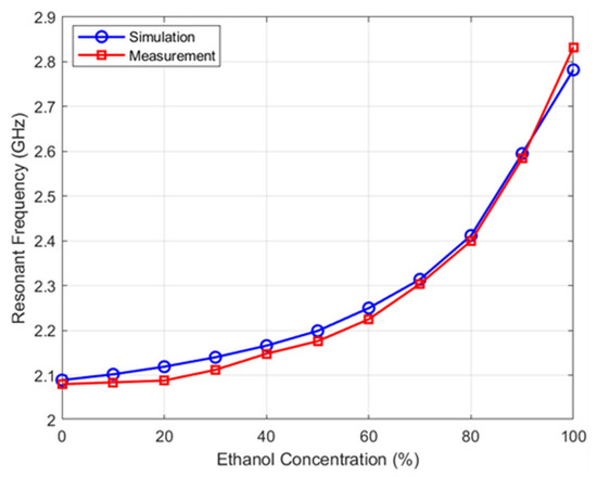
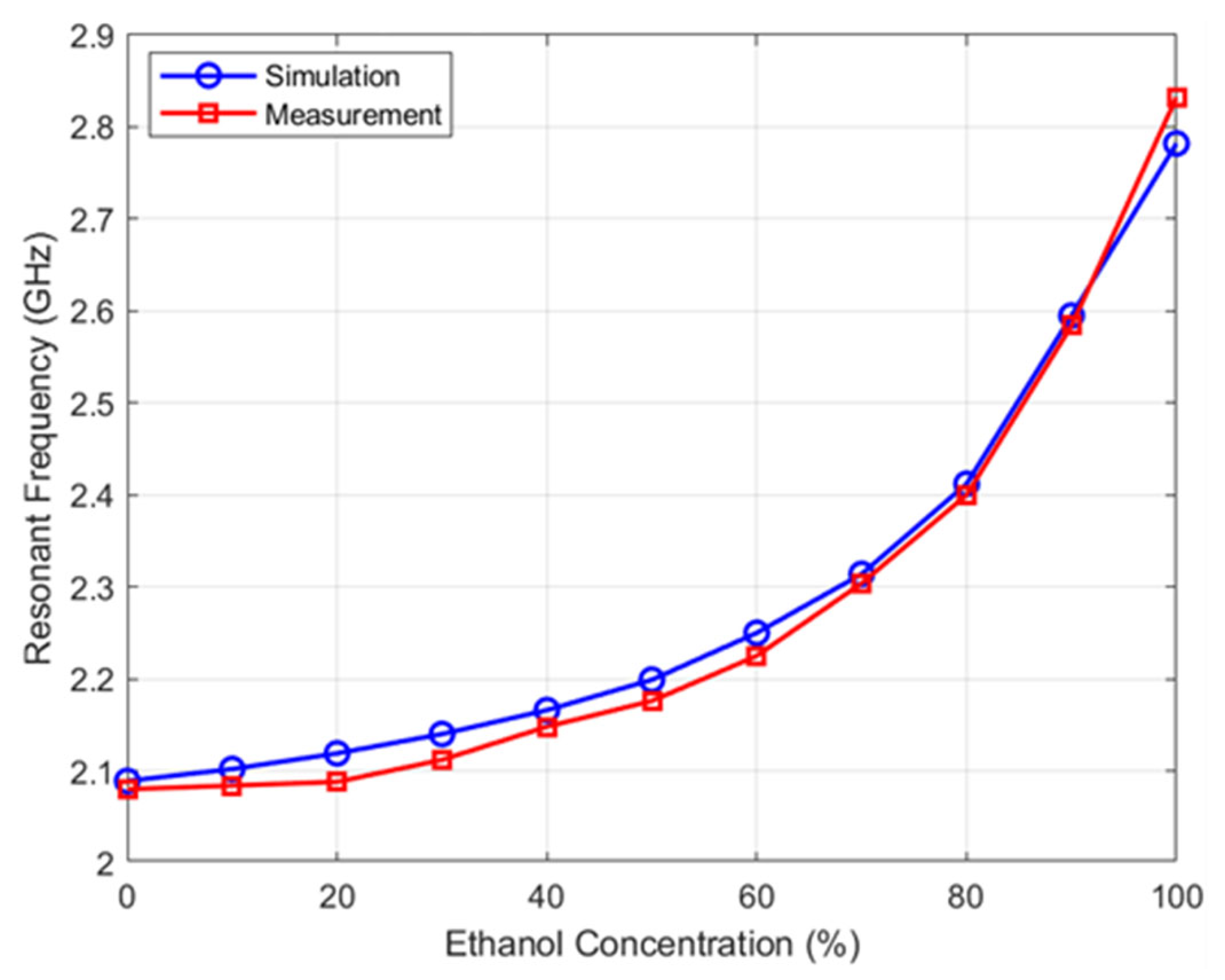
Figure 12 presents the resonant frequency as a function of ethanol concentration for both simulated and measured datasets using the data from Table 2 and Table 3, with ethanol concentration (sensor input) on the x-axis and resonant frequency (sensor output) on the y-axis. This calibration curve highlights the nonlinear increase in frequency with ethanol concentration, where the increasing slope indicates higher sensitivity at higher concentrations.

Figure 12. Resonant frequency as a function of ethanol concentration for simulated and measured datasets.

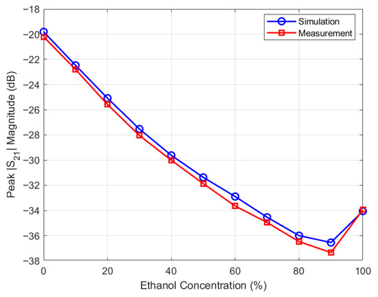
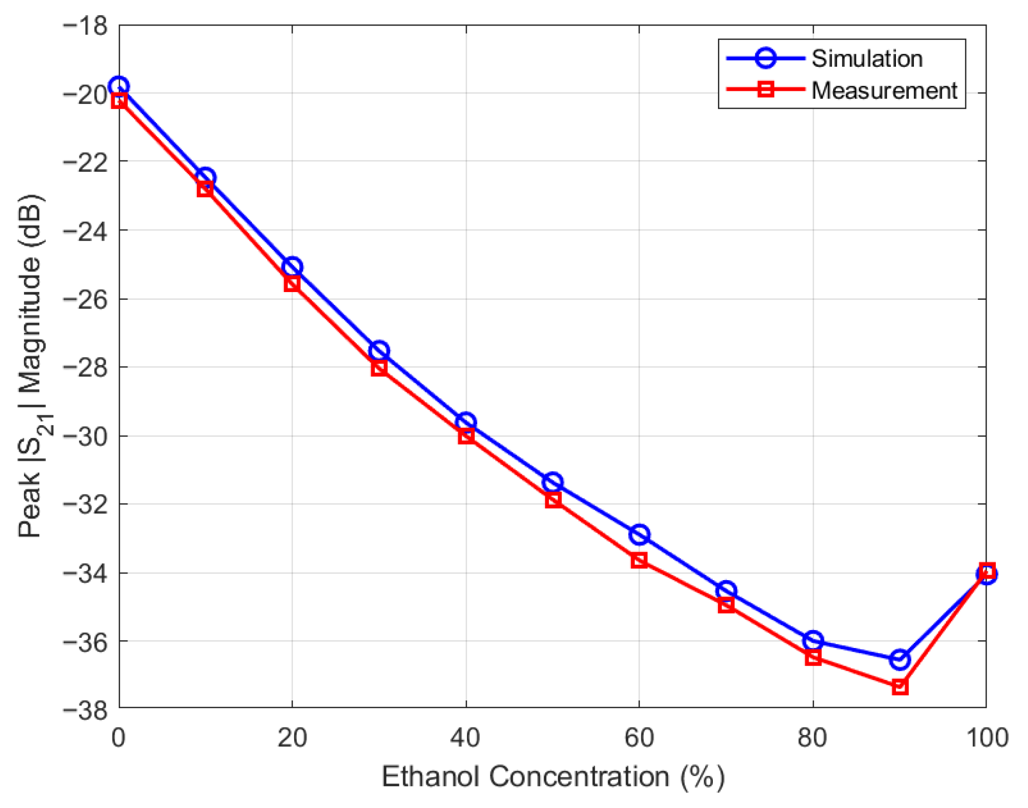
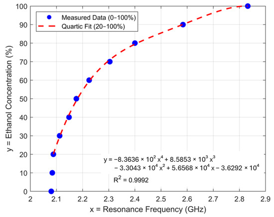
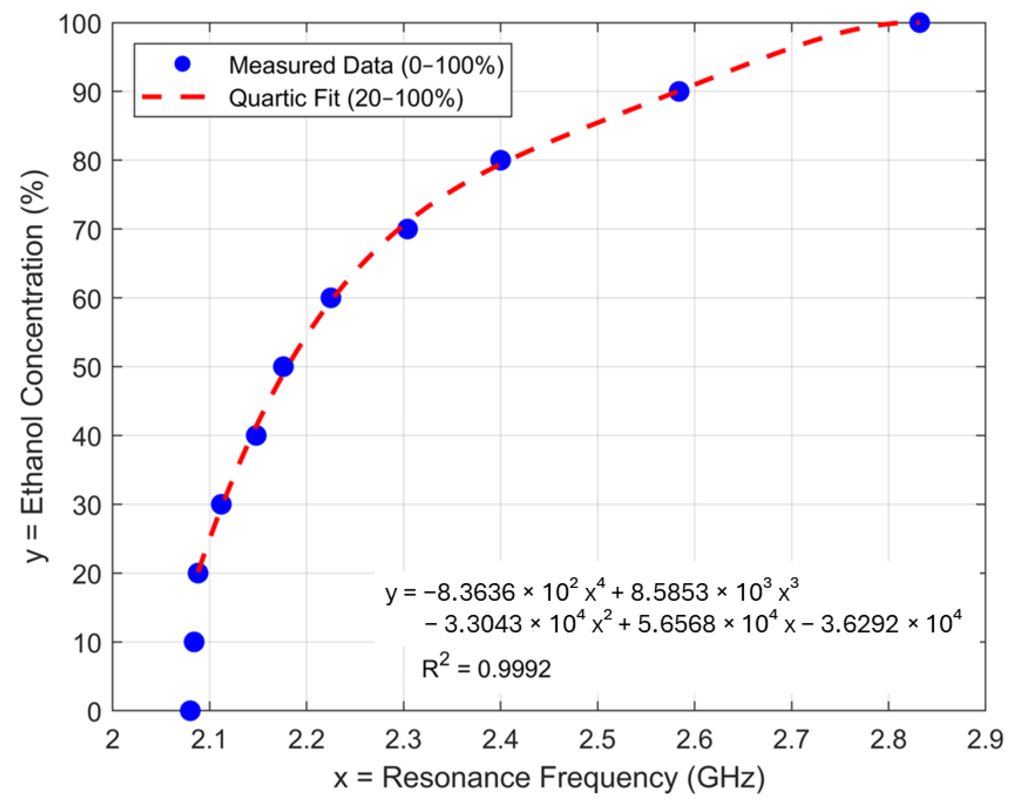
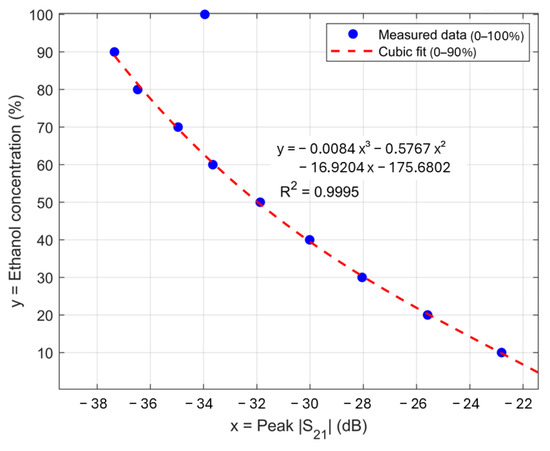
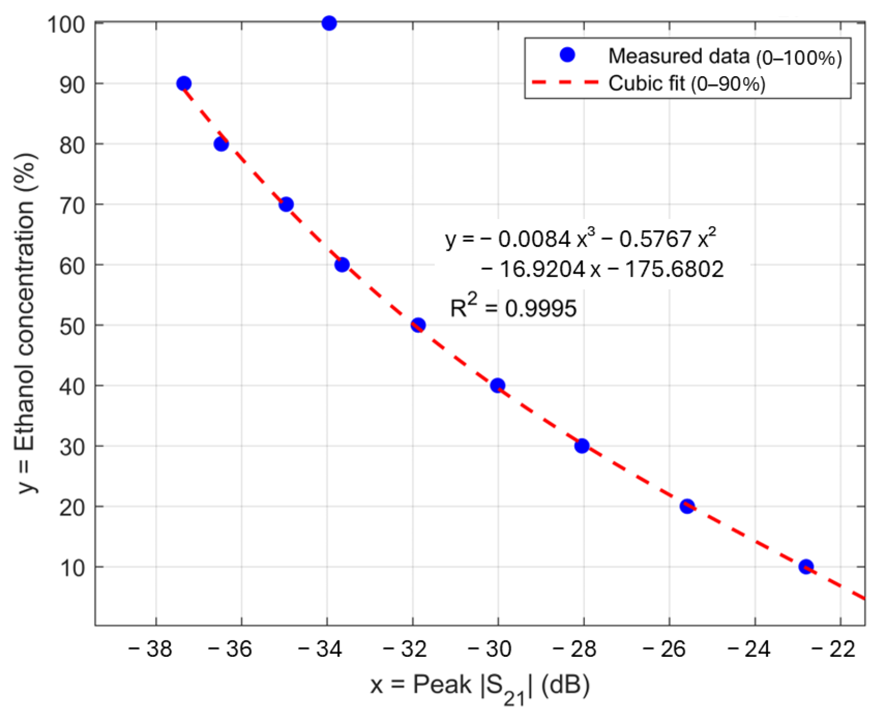
Figure 13 illustrates the simulated and measured trend of the |S₂₁|_peak as a function of ethanol concentration, showing a consistent trend for both the simulated and measured |S₂₁|_peak due to the change in ethanol concentration. As the concentration increases from 0 to 90%, |S₂₁|_peak is progressively reduced with an almost linear trend. Despite a systematic offset of |S₂₁|_peak when comparing simulated and measured data sets, both curves agree in shape and slope. As discussed before, the data point of 100% ethanol does not follow the decreasing trend of |S₂₁|_peak as the concentration is increased, and thus, it should be excluded from the data set for the creation of the calibration curve. While Figure 12 and Figure 13 present the standard calibration curves (sensor response as a function of ethanol concentration), the actual concentration retrieval uses the inverse relationships. Figure 14 and Figure 15 present the corresponding inverse calibration curves used to extract ethanol concentration from measured resonant frequency and peak |S₂₁|, respectively.

Figure 13. Peak $\mid S_{21}\mid$ magnitude as a function of ethanol concentration for simulated and measured datasets.

Figure 14. Ethanol concentration as a function of resonant frequency with the quartic inverse-calibration curve fitted to the 20–100% measured data. The 0% and 10% points are plotted for completeness but excluded from the regression because the small frequency shifts make concentration estimation ambiguous in this range.

Figure 15. Ethanol concentration as a function of peak $\mid S_{21}\mid$ with the inverse cubic calibration curve fitted over the 0–90% measured range. The 100% point is shown but excluded from the regression because it deviates from the otherwise monotonic response.

The simulation result exhibits a clear and monotonic relationship between resonant frequencies and ethanol concentrations. Referring to Figure 10, the frequency shift in the low-concentration range is relatively small and becomes stronger as the concentration increases. Unlike the case with S₂₁ magnitude, the frequency–concentration plot can be used as a calibration curve up to 100% ethanol. However, low sensitivity in the low-concentration region can lead to ambiguity for the determination of concentration, as observed from the measured result in Figure 14. For low concentrations, the frequency shift due to a change in concentration is not pronounced, and the resonant peaks are sharper, so that a low-cost VNA faces a challenge to accurately resolve the resonant frequency, leading to ambiguity in concentration extraction. Thus, the resonant frequency can be used to determine high concentrations above 20%, whereas |S₂₁|_peak should be used for the entire concentration range except for 90 to 100%. By combining concentration evaluation using both resonant frequency and |S₂₁|_peak, the ethanol concentration of the mixture can be accurately determined in the entire range from 0 to 100% with good sensitivity.

To mitigate overfitting with the limited number of calibration points, several candidate models of increasing complexity (power law, exponential, linear, quadratic, cubic, and quartic polynomials) were first fitted to the measured ethanol concentration data, using ethanol concentration as the independent variable and either resonant frequency or peak $\mid S_{21}\mid$ as the dependent variable. Model selection was based on adjusted $R^2$, inspection of residuals, and prediction errors evaluated on independent validation datasets, rather than solely on the calibration points.

Among the tested models, the quartic polynomial in resonant frequency and the cubic polynomial in |S₂₁|_peak provided the lowest prediction errors and the highest adjusted $R^2$ while preserving a physically reasonable, monotonic response, and were therefore selected as the preferred calibration relationships in this work. Lower-order linear and quadratic models produced larger and more systematic errors, especially at low and high concentrations, and did not reproduce the observed nonlinear dependence as accurately as the quartic frequency-based and cubic |S₂₁|_peak-based models.

For the resonant-frequency-based calibration, the measured concentration–frequency data in the 20–100% range (20, 30, …, 100%) were used as the calibration set [43,44,45,46], while additional measurements at 25, 35, 45, 55, 65, 75, 85, and 95% were used as an independent validation set and not for fitting. The data points of 0 and 10% were omitted due to potential ambiguity. The resulting calibration equation for ethanol concentration as a function of resonant frequency is summarized in Table 4 and was used in subsequent ethanol concentration extraction from the measured resonant frequency of an unknown mixture.

Table 4. Quartic calibration equation for ethanol concentration (%) as a function of resonant frequency (GHz) fitted to the measured data, with corresponding coefficients of determination ($R^2$).

Data Source	Regression Model for % Ethanol vs. Frequency	R2
Measurement	$y=-836.36x^4+8585.3x^3-\mathrm{33,043}{x}^2+\mathrm{56,568}x-\mathrm{36,292}$	0.9992

Note: $y$ is ethanol concentration (%) and $x$ is the resonant frequency (GHz).

On this basis, the frequency sensitivity of the sensor was evaluated in terms of the change in resonant frequency per unit change in ethanol concentration. The resonance-frequency response was modeled with a global linear relation:

$$f_r\left(y\right)\approx ay+b$$

(6)

where $y$ is the ethanol concentration in % and $f_r\left(y\right)$ is the resonant frequency in GHz as a function of $y$. The coefficient $a$ is the slope of the best-fit straight line. The average sensitivity $S$ is therefore given by the slope:

$$S=a= {\displaystyle \frac{{df}_r}{dy}}\approx 0.00837\mathrm{GHz}/\% ethanol\approx 8.4\mathrm{MHz}/\% ethanol$$

(7)

obtained from the linear fit over the 20–100% concentration range. To examine how sensitivity varies with concentration, a local, differential sensitivity was additionally defined as

$$S\left(y\right)={\displaystyle \frac{d{f}_r}{dy}}={\left({\displaystyle \frac{dy}{d{f}_r}}\right)}^{-1}$$

(8)

To rigorously assess the calibration accuracy, the mean absolute error (MAE), root mean square error (RMSE), and mean relative percent error (MRPE) were calculated between the experimentally prepared ethanol concentrations and the quartic fit-predicted concentrations for both the 20–100% calibration points and the independent 25–95% validation points. For each calibration point i, the absolute error was defined as

$${Abs Error}_i=|y_{true,i}-y_{pred,i}|$$

(9)

where $y_{\mathrm{true},i}$ is the experimentally prepared concentration, and $y_{\mathrm{pred},i}$ is the fit-predicted concentration at the corresponding resonant frequency. The MAE was then obtained as

$$MAE={\displaystyle \frac{1}{N}}\sum _{i=1}^{N}Abs {Error}_i$$

(10)

Relative accuracy was further characterized by MRPE at each nonzero concentration with

$${Relative Percent Error}_i={\displaystyle \frac{y_{pred,i}-y_{true,i}}{y_{true,i}}}\ast 100\%$$

(11)

and the corresponding mean relative percent error,

$$MRPE={\displaystyle \frac{1}{N-1}}\sum _{i=2}^{N}Relative Percent {Error}_i$$

(12)

And the root mean square error (RMSE) is obtained from

$$RMSE=\sqrt{{\displaystyle \frac{1}{N}}\sum _{i=2}^N{\left(C_{true,i}-{\widehat{C}}_i\right)}^2}$$

(13)

where $C_{\mathrm{true},i}$ is the experimentally prepared concentration, ${\widehat{C}}_i$ is the fit-predicted concentration at the corresponding resonant frequency, and $N$ is the number of points in the calibration or validation set.

Table 5 lists the true ethanol concentrations, the predicted values from the measured quartic calibration, and the resulting absolute and relative percent errors at each calibration point in the 20–100% range (with 0% and 10% shown for completeness but excluded from the fit). This comprehensive summary enables direct assessment of both individual calibration-point accuracy and the overall reliability of the resonant frequency-based extraction method within the calibrated range. For the 20–100% calibration range, the quartic model yields ${\mathrm{M}\mathrm{A}\mathrm{E}}_{20–100}$ ≈ 0.58% and ${\mathrm{R}\mathrm{M}\mathrm{S}\mathrm{E}}_{20–100}$ ≈ 0.73% ethanol concentration, and the calculated ${\mathrm{M}\mathrm{R}\mathrm{P}\mathrm{E}}_{20–100}$ in this range is approximately 1.65%, which, together with the low MAE, indicates strong agreement between the experimental results and the quartic calibration model.

Table 5. Absolute and relative errors for ethanol concentration quantification based on the resonant-frequency calibration using the quartic polynomial fit. Error metrics are calculated from the data set used to establish the calibration fit.

True (%)	Predicted (%)	Absolute Error (% of Ethanol)	Relative Error (%)
0	-	-	-
10	-	-	-
20	20.14	0.14	0.69
30	29.49	0.51	1.70
40	41.33	1.33	3.33
50	48.95	1.05	2.09
60	59.53	0.47	0.78
70	71.03	1.03	1.47
80	79.44	0.56	0.70
90	90.10	0.10	0.11
100	99.99	0.01	0.01

To further evaluate the predictive capability of the resonant-frequency-based calibration, the quartic model was applied to an independent validation set consisting of ethanol–water mixtures at 25–95% that were not used for fitting. Table 6 summarizes the true ethanol concentrations, measured resonant frequencies, quartic-predicted concentrations, and the corresponding absolute and relative percent errors for these validation points.

Table 6. Absolute and relative errors for ethanol concentration quantification on the independent validation set (25–95%) obtained by applying the quartic resonant-frequency calibration model without refitting.

True (%)	Resonant Frequency (GHz)	Predicted (%)	Absolute Error (% of Ethanol)	Relative Error (%)
25	2.092	21.84	3.16	12.63
35	2.124	33.78	1.22	3.50
45	2.152	42.57	2.43	5.41
55	2.196	53.74	1.26	2.30
65	2.260	65.42	0.42	0.64
75	2.348	75.51	0.51	0.68
85	2.520	86.71	1.71	2.01
95	2.760	99.05	4.05	4.26

For these independent validation points at 25–95%, the quartic calibration model yields a mean absolute error ${\mathrm{M}\mathrm{A}\mathrm{E}}_{25–95}$ ≈ 1.85%, ${\mathrm{R}\mathrm{M}\mathrm{S}\mathrm{E}}_{25–95}$ ≈ 2.20% and a mean relative percent error ${\mathrm{M}\mathrm{R}\mathrm{P}\mathrm{E}}_{25–95}$ ≈ 3.93% ethanol concentration. These values confirm that the frequency-based calibration retains relatively good predictive accuracy for unseen ethanol concentrations within the calibrated range. However, at an ethanol concentration of 25%, the calibration model predicts a concentration of 21.84%, resulting in a relative error of 12.63%. This increased error, compared with other concentration levels, is attributed to the reduced sensitivity at low ethanol concentrations, as discussed above.

In addition to these statistical error metrics, the main measurement-uncertainty contributions were considered qualitatively. The first contribution is frequency-reading uncertainty, determined by the VNA sweep settings (1.8–3.5 GHz span, 501 points, giving an effective frequency step of approximately 3.4 MHz) and residual peak-picking error; together, these correspond to a concentration uncertainty that remains well below 1% in the high-sensitivity region of the calibration curve. A second contribution is sample-concentration uncertainty arising from volumetric preparation of the ethanol–water mixtures using calibrated glassware, which is estimated to contribute on the order of 0.5–1% relative uncertainty in ethanol concentration for each calibration point. A third contribution is due to temperature effects, since the permittivity of ethanol–water mixtures depends on temperature; all measurements were performed at $25\pm 0.5 °\mathrm{C}$, monitored with a thermometer, so the residual temperature-induced variation in resonant frequency and $\mid S_{21}\mid$ is expected to contribute less than 1% additional concentration uncertainty over the calibration range [47]. These contributions are consistent with, and smaller than, the observed MAE and MRPE values for both the quartic (frequency-based) and cubic ($\mid S_{21}\mid$-based) calibration models, supporting the metrological robustness of the proposed sensing approach [48].

An alternative calibration strategy was developed using |S₂₁|_peak to provide ethanol quantification at low to intermediate concentrations. The calibration curve was modeled using a cubic polynomial, with the function and corresponding coefficients of the regression curve provided in Table 7. Figure 15 shows the measured ethanol concentration as a function of |S₂₁|_peak together with a calibration curve fitted over the 0–90% range, with the 100% point displayed but excluded from the regression. The response is strictly monotonic over this interval, allowing the extraction of ethanol concentration from the measured |S₂₁|_peak.

Table 7. Cubic calibration equations for ethanol concentration (%) as a function of |S₂₁|(dB) from the measured data, with corresponding coefficients of determination ($R^2$).

Data Source	Regression Model for % Ethanol vs. |S21|peak	R2
Measurement	$y=-0.0084x^3-0.5767x^2-16.9204x-175.6802$	0.9995

Note: $y$ is the ethanol concentration (%) and $x$ is the |S₂₁|(dB).

Using the previously defined error metrics in Equations (10), (12) and (13), the cubic |S₂₁|_peak based calibration over the 0–90% ethanol calibration set yields a ${\mathrm{M}\mathrm{A}\mathrm{E}}_{0–90}$ ≈ 0.52% ethanol concentration and a mean relative percent error ${\mathrm{M}\mathrm{R}\mathrm{P}\mathrm{E}}_{0–90}\approx 1.22\%$, together with ${\mathrm{R}\mathrm{M}\mathrm{S}\mathrm{E}}_{0–90}$≈ 0.65%. Table 8 lists the true ethanol concentrations as prepared, the corresponding values predicted by the cubic calibration, and the associated absolute and percent errors, confirming that individual deviations remain lower than about 1.5% ethanol concentration over the 0–90% calibration range. Low MAE, RMPE, and RMSE confirm that |S₂₁|_peak can serve as a reliable parameter for the extraction of ethanol concentration, especially in the low-to-intermediate concentration regime where resonant peaks are more pronounced.

Table 8. Absolute and relative errors for ethanol concentration quantification based on the|S₂₁| _peak-based calibration using a cubic polynomial fit over the 0–90% calibration range. Error metrics are calculated from the data set used to establish the calibration fit.

True (%)	Predicted (%)	Absolute Error (% of Ethanol)	Relative Error (%)
25	0.02	0.02	NA
35	9.81	0.19	1.94
45	20.27	0.27	1.36
55	30.38	0.38	1.26
65	39.56	0.44	1.10
50	49.48	0.52	1.04
60	60.45	0.45	0.74
70	69.57	0.44	0.62
80	81.46	1.46	1.83
90	89.01	0.99	1.10
100	-	-	-

The calibration model was subsequently applied to an independent validation data set covering ethanol concentrations from 5% to 85%, which was not used during model fitting. The corresponding prediction errors of the cubic $\mid S_{21,\mathrm{peak}}\mid$-based model are summarized in Table 9. This model achieves an ${\mathrm{M}\mathrm{A}\mathrm{E}}_{5–85}$ of approximately 0.55%, ${\mathrm{R}\mathrm{M}\mathrm{S}\mathrm{E}}_{5–85}$ of approximately 0.75%, and an ${\mathrm{M}\mathrm{R}\mathrm{P}\mathrm{E}}_{5–85}$ of approximately 1.20%, with all individual relative errors remaining below 3.2%. Overall, these results demonstrate that the cubic $\mid S_{21,\mathrm{peak}}\mid$-based calibration model provides excellent predictive accuracy in the low-to-intermediate ethanol concentration range, outperforming the quartic resonant-frequency-based model from Table 4.

Table 9. Absolute and relative errors for ethanol concentration quantification on the independent validation set (5–85% ethanol) using the |S₂₁| _peak-based cubic calibration model.

True (%)	|S21|peak(dB)	Predicted (%)	Absolute Error (% of Ethanol)	Relative Error (%)
5	−21.491	4.98	0.02	0.46
15	−24.200	15.10	0.10	0.69
25	−26.927	25.79	0.79	3.16
35	−29.053	35.12	0.12	0.35
45	−31.115	45.51	0.51	1.13
55	−32.952	56.24	1.24	2.25
65	−34.207	64.53	0.47	0.72
75	−35.653	75.20	0.20	0.27
85	−37.019	86.52	1.52	1.79

As seen in Table 9, all absolute errors remain below 1.6% ethanol and all relative errors below 3.2%, supporting the robustness of the |S₂₁| _peak-based calibration in the validation set.

3.5. Comparison of the Proposed Cavity Resonator with Previously Reported Cavity Resonators

To benchmark the performance of the proposed cavity resonator against the state of the art, Table 10 presents a comparison with previously reported cylindrical (or cavity-based) microwave resonators. The table summarizes key parameters, including operating frequency, cavity dimensions, air-filled and water-loaded Q-factors, fabrication materials and techniques, and sample loading methods.

Table 10. Performance comparison of the proposed 3D-printed cylindrical cavity resonator with the previously reported cylindrical cavity resonator in the literature.

Ref.	Freq. (Air) (GHz)	$\mathbf{Diameter} \times$ Height (mm)	Q-Factor (Air-Filled)	Q-Factor (Water Loaded)	Material	Production	LUT Feeding Method
[2]	1.5	-	-	-	Metal	CNC machining	Standard laboratory test tubes
[3]		$\mathrm{\varnothing }38\times 20$	-	-	Metal	Precision machining	Nonconductive tube
[4]	10.3	$\varnothing 11.3\times 30$	3818	-	Aluminum	Mechanical fabrication	Metal cavity body
[7]	3.0	$\varnothing 77.66\times 40$	445.58	23.912	Aluminum	CNC machining	The PTFE tube penetrates from top to bottom.
[49]	2.4–2.5	$\varnothing 92\times 40$	2010.40	213.18	Metal	CNC machining and glass/quartz tube fabrication	Quartz tube
This work	3.0	$\varnothing 76.6\times 40$	250.58 (simulated) 200.26 (measured)	46.5 (simulated) 37.3 (measured)	PLA, Copper tape	3D printing	Standard centrifuge tube

Across the literature, the air-filled cavities typically exhibit high Q-factors, ranging from several hundred to several thousand, while the introduction of water or aqueous samples consistently leads to a pronounced reduction in Q-factor due to increased dielectric loss. For example, a 10.3 GHz cylindrical cavity designed for low-loss liquid characterization achieves a simulated air-filled Q-factor of 3818 [4], whereas a CNC-machined aluminum cavity operating at 3.0 GHz exhibits a measured Q of 445.6 in air that decreases to 23.9 when loaded with water using a PTFE tube [7]. A similar trend is observed for a cavity with the resonant frequency of 2.5 GHz, where the air-filled Q-factor of 2010.40 is reduced to 213.18 under water-loading conditions [49]. As discussed above, the lower Q-factor of the proposed 3D-printed cavity compared with those reported in the literature is primarily due to the larger opening required to accommodate insertion of the standard centrifuge tube containing the liquid under test.

Within this established context, the proposed resonator demonstrates performance consistent with prior work while employing a markedly different and lower-cost fabrication approach. The proposed TM₀₁₀ cylindrical cavity is fabricated using FDM 3D printing with PLA and lined with copper tape, operating near 3.0 GHz. The air-filled cavity exhibits a Q-factor of 250.6 in simulation and 200.3 in measurement, while loading with deionized water using a standard 1.5 mL centrifuge tube as a modular sample holder reduces the Q-factor to 46.5 (simulation) and 37.3 (measurement). This substantial reduction is consistent with the high dielectric loss of water at a few gigahertz, which introduces a strong dielectric-loss contribution to the total Q of the TM₀₁₀ mode. In terms of the usual relation $1/Q_{\mathrm{total}}=1/Q_{\mathrm{cond}}+1/Q_{\mathrm{dielectric}}+1/Q_{\mathrm{rad}}$, the empty cavity Q is dominated by conductor and coupling-port losses, whereas inserting the lossy water sample adds a low $Q_{\mathrm{dielectric}}$ term that significantly lowers $Q_{\mathrm{total}}$. In the present design, additional loss arises from the large sample opening in the top endcap (used to accommodate the centrifuge tube), which slightly increases radiation/coupling loss, and from the finite conductivity and surface roughness of the copper-tape metallization compared with bulk metal, both of which further reduce $Q_{\mathrm{cond}}$. The close agreement between simulation with idealized copper walls and measurement for both air-filled and water-loaded cases indicates that the observed Q-factor values are physically consistent with these combined loss mechanisms.

Compared to the simulated Q-factor without practical losses, e.g., surface roughness, conductive loss of the copper tape, and fabrication tolerance, the Q-factor of the fabricated cavity can be further improved, e.g., by surface treatment of the 3D-printed cavity. It is observed that, even in simulation, the Q-factor of the proposed cavity is lower than the one reported in [7], fabricated by CNC machining. The decrease in Q-factor is not attributed to the use of 3D printing as the fabrication method, but rather to the substantially larger insertion opening required to accommodate a standard centrifuge tube compared with the 4 mm PTFE tube in [7]. The larger opening increases radiation loss and consequently reduces the Q-factor. This design choice is intentional, as it enables the use of widely adopted laboratory sample containers. Despite the reduced Q-factor, the resonance peaks remain well defined, allowing reliable extraction of both the resonant frequency and |S₂₁|_peak, as demonstrated in the ethanol concentration sensing experiments.

Beyond resonator performance, additive manufacturing provides substantial design flexibility. In particular, the customized cavity top endcap functions as a sample holder, enabling direct integration of liquids contained in standard centrifuge tubes commonly used in chemical and biomedical laboratories. Using this platform, ethanol concentration sensing in ethanol–DI water mixtures is successfully demonstrated with good accuracy, even when measurements are performed using a low-cost vector network analyzer rather than a high-end laboratory instrument. Thus, the proposed approach combines competitive Q-factor performance with low fabrication cost, ease of assembly, and high customizability, providing an accessible microwave liquid characterization tool for small laboratories and resource-limited research environments.

4. Conclusions

This work presents a low-cost, highly customizable cylindrical microwave cavity resonator fabricated using FDM 3D printing with PLA and copper-tape metallization. Operating in the TM₀₁₀ mode around 3 GHz, the resonator integrates a standard 1.5 mL centrifuge tube as a modular sample holder, enabling practical liquid measurements compatible with chemical and biomedical laboratories. Despite its additively manufactured structure and inexpensive materials, the cavity exhibits well-defined resonant behavior, with air-filled and water-loaded Q-factors comparable to those reported for conventionally machined metal cavities.

To demonstrate the applicability of the proposed 3D-printed cavity resonator, experiments were performed by measuring the cavity transmission coefficient for ethanol–deionized water mixtures with varying ethanol concentrations. The measured relationships between ethanol concentration and both the resonant frequency and peak magnitude were fitted using polynomial regression. Using a combination of regression models for resonant frequency and peak magnitude, the ethanol concentration of the mixture can be extracted from 0 to 100% with good accuracy. The successful use of a low-cost vector network analyzer further highlights the accessibility of the proposed sensing platform.

Compared with prior cavity resonator-based liquid sensors, the proposed approach offers significant advantages in fabrication cost, design flexibility, and sample handling by leveraging additive manufacturing and standard laboratory containers. Beyond ethanol sensing, the presented design and methodology provide a general framework for microwave dielectric characterization of liquids, with potential extensions to chemical engineering, biomedical research, and educational applications.

References

- Chudpooti, N.; Pechrkool, T.; Sangpet, P.; Akkaraekthalin, P.; Robertson, I.D.; Somjit, N. 5.58-GHz modified Jerusalem patch sensor for 1%-precision ethanol and methanol discrimination in disinfectant solutions. IEEE Access 2024, 12, 112690–112701. [Google Scholar] [CrossRef] [Scilit]
- Avalos Ribas, R.; Gelosi, I.E.; Uriz, A.J.; Moreira, J.C.; Bonadero, J.C. A high-sensitivity cylindrical cavity resonator sensor for the characterization of aqueous solutions. IEEE Sens. J. 2021, 21, 7581–7589. [Google Scholar] [CrossRef] [Scilit]
- Li, Z.; Meng, Z.; Fei, F.; Gibson, A. Microwave cylindrical cavity resonator sensor for detection and characterization of contaminants in lubricating oil. IEEE Sens. J. 2022, 22, 22600–22609. [Google Scholar] [CrossRef] [Scilit]
- Li, C.; Mousavi, S.; Asadi, R.; Mousavi, S.; Vahdani, R.; Ye, X.; Wang, K.; Kim, D.B. Dk and Df characterization of low-loss dielectric liquid by cylindrical cavity resonator. In Proceedings of the 2024 IEEE International Symposium on Electromagnetic Compatibility, Signal & Power Integrity (EMC+SIPI), Phoenix, AZ, USA, 5–9 August 2024; pp. 119–124. [Google Scholar] [CrossRef] [Scilit]
- Hussain, N.S.M.; Azman, A.N.; Yusof, N.A.T.; Mohtadzar, N.A.A.H.; Karim, M.S.A. Design of resonator cavity for liquid material characterization. Telkomnika 2022, 20, 2. [Google Scholar] [CrossRef] [Scilit]
- Cole, A.J.; Young, P.R. Chipless liquid sensing using a slotted cylindrical resonator. IEEE Sens. J. 2018, 18, 149–156. [Google Scholar] [CrossRef] [Scilit]
- Kanpan, P.; Khansalee, E.; Puangngernmak, N.; Chalermwisutkul, S. TM010 mode cylindrical cavity for complex permittivity measurement of liquid using field analysis technique. In Proceedings of the 2012 9th International Conference on Electrical Engineering/Electronics, Computer, Telecommunications and Information Technology, Phetchaburi, Thailand, 16–18 May 2012; IEEE: Piscataway, NJ, USA, 2012; pp. 1–4. [Google Scholar] [CrossRef] [Scilit]
- Ozbey, B.; Faz, U.; Wolf, B.; Eibert, T.F. Ultrasensitive moisture content characterization of wood samples by a cylindrical cavity resonator. Sens. Actuators A Phys. 2020, 315, 112298. [Google Scholar] [CrossRef] [Scilit]
- Kittiamornkul, N.; Chamnongthai, K.; Jirasereeamornkul, K.; Higuchi, K. A System of Microwave Cylindrical Cavity Resonator for Granular Material Dielectric Measurement Using Two Waveguide Transmitters. In Proceedings of the SICE Annual Conference; SICE: Tokyo, Japan, 2010. [Google Scholar]
- Mousavi, M.; Li, C.; Asadi, R.; Mousavi, S.; Vahdani, R.; Ye, X.; Esmaeelpour, M.; Kim, D.B. Analytical Modeling of Partially-Filled TM010-Mode Dielectric Resonator for Accurate DK and DF Extraction. In Proceedings of the IEEE International Symposium on Electromagnetic Compatibility, Signal & Power Integrity (EMC+SIPI), Phoenix, AZ, USA, 5–9 August 2024; IEEE: Piscataway, NJ, USA, 2024; pp. 130–134. [Google Scholar] [CrossRef] [Scilit]
- Asadi, R.; Li, C.; Mousavi, S.; Mousavi, S.M.; Vahdani, R.; Ye, X.; Kim, D.B. Design of the TM010 Mode Cylindrical Cavity Resonator for PCB Dielectric Characterization. In Proceedings of the IEEE International Symposium on Electromagnetic Compatibility, Signal & Power Integrity (EMC+SIPI), Phoenix, AZ, USA, 5–9 August 2024; IEEE: Piscataway, NJ, USA, 2024; pp. 125–129. [Google Scholar] [CrossRef] [Scilit]
- Li, Y.; Zhao, J.; Zhang, S.; Yang, Z.; Zhao, H. A Microwave Cavity Resonator-Based System for Wetness Measurement in Steam Turbine. In Proceedings of the IEEE International Conference on Mechatronics and Automation (ICMA), Luoyang, China, 25–28 June 2006; IEEE: Piscataway, NJ, USA, 2006. [Google Scholar] [CrossRef] [Scilit]
- Tameishi, A.; Kamijo, T.; Suzuki, Y.; Kik, A.; Taki, M.; Sasaki, K. Complex Permittivity Measurement Method of High-Loss Materials Using Cylindrical Cavity Resonator in Millimeter-Wave Band. In Proceedings of the IEEE International Symposium on Electromagnetic Compatibility, Tokyo, Japan, 12–16 May 2014; IEEE: Piscataway, NJ, USA, 2014. [Google Scholar]
- Zhang, Z.; Chen, C.; Wu, X. A Compact Cavity Filter with Novel TM Mode Dielectric Resonator Structure. In Proceedings of the IEEE International Conference on Microwave Technology and Computational Electromagnetics (ICMTCE), Beijing, China, 22–25 May 2011; IEEE: Piscataway, NJ, USA, 2011. [Google Scholar] [CrossRef] [Scilit]
- Annino, G.; Cassettari, M.; Martinelli, M. A New Concept of Open TE011 Cavity. IEEE Trans. Microw. Theory Tech. 2009, 57, 775–783. [Google Scholar] [CrossRef] [Scilit]
- Mohammed, A.M.; Wang, Y.; Skaik, T.; Hanham, S.M. Millimeter-Wave Re-Entrant Cavity Resonator Sensor for Liquid Dielectric Metrology. In Proceedings of the 54th European Microwave Conference (EuMC), Paris, France, 24–26 September 2024; IEEE: Piscataway, NJ, USA, 2024; pp. 433–436. [Google Scholar] [CrossRef] [Scilit]
- Lamba, O.S.; Kaushik, M.; Joshi, L.M.; Meena, R.; Pal, D.; Jindal, V.; Jangir, P.; Singh, V.; Kumar, S.; Kant, D. Simulation and Characterization of Cylindrical RF Cavity with Output Section Coupling for 250 kW CW C-Band Klystron. In Proceedings of the IEEE International Vacuum Electronics Conference (IVEC), Bangalore, India, 21–24 February 2011; IEEE: Piscataway, NJ, USA, 2011. [Google Scholar] [CrossRef] [Scilit]
- Penaranda-Foix, F.L.; Catala-Civera, J.M.; Canos-Marin, A.J.; Garcia-Banos, B. Frequency Deviation Due to a Sample Insertion Hole in a Cylindrical Cavity by Circuital Analysis. In Proceedings of the IEEE MTT-S International Microwave Symposium Digest, Honolulu, HI, USA, 3–8 June 2007; IEEE: Piscataway, NJ, USA, 2007. [Google Scholar] [CrossRef] [Scilit]
- Ye, M.; Jiang, L.; Xiang, F.; Yang, F.; He, Y. Lift-Off and Tilt Effect in Microwave Surface Resistance Measurement Using TE011-Mode Cylindrical Cavity. IEEE Trans. Instrum. Meas. 2022, 71, 8002308. [Google Scholar] [CrossRef] [Scilit]
- Rigelsford, J.M.; Cerveny, M. A Simplification Technique for S-Parameter Calculations within Partially Loaded Resonant Cavities. In Proceedings of the Progress in Electromagnetics Research Symposium (PIERS), Shanghai, China, 8–11 August 2016; IEEE: Piscataway, NJ, USA, 2016. [Google Scholar] [CrossRef] [Scilit]
- Ertay, A.O.; Köseoğlu, E.; Şimşek, S.; Demiralay, B. Comparative Analysis of Dielectric Loading Effects for Rectangular Cavity Resonators. In Proceedings of the 4th International Electromagnetic Compatibility Conference (EMC Türkiye), Ankara, Turkey, 24–27 September 2017; IEEE: Piscataway, NJ, USA, 2017. [Google Scholar] [CrossRef] [Scilit]
- Carter, R.G.; Feng, J.; Becker, U. Calculation of the Properties of Reentrant Cylindrical Cavity Resonators. IEEE Trans. Microw. Theory Tech. 2007, 55, 12. [Google Scholar] [CrossRef] [Scilit]
- Saydam, T.; Biskin, O.S.; Aksoy, S. Low-Frequency Excitation of a Lossy Dielectric-Filled Cavity Resonator Using QS-FDTD Method. In Proceedings of the Workshop on Microwave Theory and Techniques in Wireless Communications (MTTW), Riga, Latvia, 5–7 October 2022; IEEE: Piscataway, NJ, USA, 2022. [Google Scholar] [CrossRef] [Scilit]
- Vyas, A.D.; Rana, V.A.; Gadani, D.H.; Prajapati, A.N. Cavity Perturbation Technique for Complex Permittivity Measurement of Dielectric Materials at X-Band Microwave Frequency. In Proceedings of the International Conference on Recent Advances in Microwave Theory and Applications (AMTA), Jaipur, India, 21–24 November 2008; IEEE: Piscataway, NJ, USA, 2008. [Google Scholar] [CrossRef] [Scilit]
- Zhang, Y.; Xu, L.; Chen, J.; Bai, X.; Zhou, X. High sensitivity detection of ethanol solution based on waveguide resonant cavity combined with metamaterials. Measurement 2024, 225, 114030. [Google Scholar] [CrossRef] [Scilit]
- Ds, C.; Nagini, K.B.S.S.; Barik, R.K.; Koziel, S. Highly sensitive microwave sensors based on open complementary square split-ring resonator for sensing liquid materials. Sensors 2024, 24, 1840. [Google Scholar] [CrossRef] [Scilit] [PubMed]
- Salim, A.; Ghosh, S.; Lim, S. Low-cost and lightweight 3D-printed split-ring resonator for chemical sensing applications. Sensors 2018, 18, 3049. [Google Scholar] [CrossRef] [Scilit] [PubMed]
- Omer, A.E.; Shaker, G.; Safavi-Naeini, S.; Kokabi, H.; Alquié, G.; Deshours, F.; Shubair, R.M. Low-cost portable microwave sensor for non-invasive monitoring of blood glucose level: Novel design utilizing a four-cell CSRR hexagonal configuration. Sci. Rep. 2020, 10, 15200. [Google Scholar] [CrossRef] [Scilit] [PubMed]
- Kyovtorov, V.; Georgiev, I.; Margenov, S.; Stoychev, D.; Oliveri, F.; Tarchi, D. New antenna design approach: 3D polymer printing and metallization—Experimental test at 14–18 GHz. AEU Int. J. Electron. Commun. 2017, 73, 119–128. [Google Scholar] [CrossRef] [Scilit]
- Bozzi, M.; Tomassoni, C.; Perregrini, L.; Bahr, R.; Tentzeris, M. Additive manufacturing of substrate integrated waveguide components. In Proceedings of the 2016 IEEE MTT-S International Microwave Workshop Series on Advanced Materials and Processes for RF and THz Applications (IMWS-AMP), Chengdu, China, 20–22 July 2016; pp. 1–4. [Google Scholar]
- Chan, K.Y.; Ramer, R.; Sorrentino, R. Low-cost Ku-band waveguide devices using 3-D printing and liquid metal filling. IEEE Trans. Microw. Theory Tech. 2018, 66, 3993–4001. [Google Scholar] [CrossRef] [Scilit]
- Pourafzal, A.; Roi-Taravella, T.; Cheffena, M.; Yayilgan, S.Y. A low-cost and accurate microwave sensor system for permittivity characterization. IEEE Sens. J. 2023, 23, 1234–1248. [Google Scholar] [CrossRef] [Scilit]
- Pozar, D.M. Microwave Engineering, 4th ed.; Wiley: Hoboken, NJ, USA, 2011. [Google Scholar]
- Krupka, J.; Derzakowski, K.; Abramowicz, A.; Tobar, M.E.; Geyer, R.G. Use of Whispering-Gallery Modes for Complex Permittivity Determinations of Ultra-Low-Loss Dielectric Materials. IEEE Trans. Microw. Theory Tech. 1999, 47, 752–759. [Google Scholar] [CrossRef] [Scilit]
- Phakaew, T.; Oo, T.P.; Uzair, M.; Kowitwarangkul, P.; Chuchuay, P.; Yeetsorn, R.; Torrungrueng, D.; Chudpooti, N.; Chalermwisutkul, S. Additively Manufactured Mechanically Tunable Cavity Resonator for Broadband Characterization of Liquid Permittivity. Sensors 2025, 25, 7145. [Google Scholar] [CrossRef] [Scilit]
- Koirala, G.R.; Dhakal, R.; Kim, E.-S.; Yao, Z.; Kim, N.-Y. Radio Frequency Detection and Characterization of Water–Ethanol Solution through Spiral-Coupled Passive Micro-Resonator Sensor. Sensors 2018, 18, 1075. [Google Scholar] [CrossRef] [Scilit]
- Moriyoshi, T.; Ishii, T.; Tamai, Y.; Tado, M. Static Dielectric Constants of Water + Ethanol Mixtures from 0.1 to 300 MPa at 298.15 K. J. Chem. Eng. Data 1990, 35, 17–20. [Google Scholar] [CrossRef] [Scilit]
- Sato, T.; Buchner, R. Dielectric Relaxation Processes in Ethanol/Water Mixtures. J. Phys. Chem. A 2004, 108, 5007–5015. [Google Scholar] [CrossRef] [Scilit]
- Wyman, J.; Jeffries, W. The Dielectric Constant of Mixtures of Ethyl Alcohol and Water from −5 to 40 °C. J. Am. Chem. Soc. 1931, 53, 3292–3301. [Google Scholar] [CrossRef] [Scilit]
- Megriche, A.; Belhadj, A.; Mgaidi, A. Microwave Dielectric Properties of Binary Solvent Water–Alcohol Mixtures. Mediterr. J. Chem. 2012, 1, 4. [Google Scholar] [CrossRef] [Scilit]
- Bohigas, X.; Tejada, J. Dielectric Characterization of Alcoholic Beverages and Ethanol–Water Solutions under Microwave Radiation. Food Res. Int. 2010, 43, 6. [Google Scholar] [CrossRef] [Scilit]
- NanoVNA|Very Tiny handheld Vector Network Analyzer. Available online: https://nanovna.com/ (accessed on 5 January 2026).
- Li, Z.; Tian, S.; Tang, J.; Yang, W.; Hong, T.; Zhu, H. High-Sensitivity Differential Sensor for Characterizing Complex Permittivity of Liquids Based on LC Resonators. Sensors 2024, 24, 4877. [Google Scholar] [CrossRef] [Scilit]
- Wójcikowski, M. Real-Time PPG Signal Conditioning with Long Short-Term Memory Network for Wearable Devices. Sensors 2022, 22, 164. [Google Scholar] [CrossRef] [Scilit]
- Mendes, L.; Carvalho, P. Adaptive Polynomial Regression for Colorimetric Scanner Calibration Using Genetic Algorithms. In Proceedings of the IEEE International Workshop on Intelligent Signal Processing, Faro, Portugal, 1–3 September 2005; IEEE: Piscataway, NJ, USA, 2005; pp. 22–27. [Google Scholar] [CrossRef] [Scilit]
- Shan, H.; Yu, L.; Wang, H.; Li, Y.; Cao, B. Calibration of Indoor EM Location System Based on Polynomial Fitting. In Proceedings of the IEEE International Conference on Electronic Information and Communication Technology (ICEICT), Harbin, China, 20–22 January 2019; IEEE: Piscataway, NJ, USA, 2019; pp. 873–876. [Google Scholar] [CrossRef] [Scilit]
- Petong, P.; Pottel, R.; Kaatze, U. Water–ethanol mixtures at different compositions and temperatures: A dielectric relaxation study. J. Phys. Chem. A 2000, 104, 7420–7428. [Google Scholar] [CrossRef] [Scilit]
- Ellison, S.L.R.; Williams, A. Eurachem/CITAC Guide: Quantifying Uncertainty in Analytical Measurement, 3rd ed.; Eurachem/CITAC: Teddington, UK, 2012; Available online: http://www.eurachem.org/ (accessed on 23 January 2026).
- Li, Z.; Meng, Z.; Haigh, A.; Wang, P.; Gibson, A. Characterisation of Water in Honey Using a Microwave Cylindrical Cavity Resonator Sensor. J. Food Eng. 2021, 292, 110373. [Google Scholar] [CrossRef] [Scilit]
Disclaimer/Publisher’s Note: The statements, opinions and data contained in all publications are solely those of the individual author(s) and contributor(s) and not of MDPI and/or the editor(s). MDPI and/or the editor(s) disclaim responsibility for any injury to people or property resulting from any ideas, methods, instructions or products referred to in the content. |
© 2026 by the authors. Licensee MDPI, Basel, Switzerland. This article is an open access article distributed under the terms and conditions of the Creative Commons Attribution (CC BY) license.