Generalized Fractional Interpolated Discrete Fourier Transform with Rectangular Window for Frequency Estimation in Noisy Sinewave Signals

Abstract

Accurate and efficient frequency estimation is essential in many scientific fields and has led to the development of various algorithms. Commonly used methods involve applying the Discrete Fourier Transform followed by spectral interpolation. This approach faces challenges especially under low signal-to-noise ratio conditions. To mitigate this limitation, the Generalized Fractional Interpolated Discrete Fourier Transform for frequency estimation of rectangular-windowed sinewaves is proposed. This non-iterative algorithm enhances frequency estimation by employing spectral components at fractional steps of the Discrete Fourier Transform frequency resolution. A non-iterative, closed-form equation for frequency estimation is derived, enabling efficient computation. The proposed algorithm is evaluated through numerical simulations and compared with existing interpolation methods for different frequencies, signal-to-noise ratios, and number of acquired samples. The method is validated using experimentally acquired sinewave signals.

1. Introduction

Frequency estimation of sinewaves is a critical task in many science and engineering domains [1,2,3]. Accurate frequency estimation plays a vital role in applications such as power quality monitoring [4,5], structural health assessment [6], radar signal processing [7], medical diagnostics [8] or communications [9,10]. For example, in power quality monitoring systems, accurate frequency tracking is essential for detecting grid disturbances, identifying harmonic distortion, and ensuring regulatory compliance with standards such as IEEE Std. 1159-2019 [11] or IEC 61000-4-30 [12]. To address the requirements of these applications, which may need real-time performance and resilience to noise, multiple frequency estimation algorithms have been proposed.

The concept of interpolation in the DFT spectrum was first introduced by Rife and Vincent [13]. A widely used, closed-form and computationally efficient implementation of a frequency interpolation algorithm was proposed by Renders et al. [14] which is referred to here as the Interpolated Discrete Fourier Transform (IpDFT). This method begins with the computation of the acquired signal Discrete Fourier Transform (DFT), followed by the spectral interpolation of two adjacent DFT lines to estimate the signal frequency. The interpolation is based on the theoretical spectral shape of a sinewave sampled with a rectangular window, allowing the algorithm to correct for the limited frequency resolution of the DFT. Besides the IpDFT algorithm presented in [14], multiple other frequency interpolation approaches have been developed, many including windowing techniques [15,16] as well as employing iterative methods [17]. In general, these interpolation techniques rely on spectral components that are spaced by the DFT frequency resolution, $\Delta f$. This dependence introduces limitations, particularly when the signal frequency is close to a DFT bin center. In those cases, the neighboring spectral components used in the interpolation have low amplitude and are therefore more susceptible to noise which increases the frequency estimation Root Mean Square Error (RMSE). Although these algorithms have the ability to provide accurate estimates, their performance is degraded under low signal-to-noise ratio (SNR) conditions.

Aboutanios and Mulgrew [18] proposed an algorithm with two variants, where two Discrete Time Fourier Transform (DTFT) coefficients located at the midpoints of DFT bins are used for interpolation—the variants use different frequency estimation equations. The Fractional Interpolated Discrete Fourier Transform (FracIpDFT) algorithm proposed in [19] uses non-integer Goertzel filters [20] to compute DTFT components at fractional frequency intervals, specifically at integer multiples of $\Delta f/2$, which are then used in the IpDFT algorithm [14] to estimate the signal frequency. Although the IpDFT algorithm was developed to use DFT spectral components, it was shown in [19] that it can be used with frequency components located at multiples of $\Delta f/2$, as long as the two components used in the interpolation are $\Delta f$ spaced. This allows the FracIpDFT algorithm to avoid the use of spectral lines with very low amplitude, and therefore to outperform conventional interpolation methods. An alternative interpolation-based frequency estimation approach was introduced by Fan et al. [21], which also uses DTFT components spaced at $\Delta f/2$. However, this method is restricted to the $\Delta f/2$ spacing value and relies on zero padding the signal to enhance frequency resolution, a process that distorts the original waveform.

Recent research has also included DTFT linearization and interpolation methods to obtain accurate frequency estimation of sinewaves [22] and iterative interpolation techniques to eliminate spectral leakage [23]. Other developments include DFT interpolation based on maximum sidelobe decay windows [24], autocorrelation followed by DTFT methods [25], and estimators optimized for short records [26]. Three-point interpolation techniques have also been extended for the frequency estimation of exponentially damped sinewaves [27,28].

This paper is an expansion of the work developed in [29] and proposes the Generalized Fractional Interpolated Discrete Fourier Transform (GFIpDFT) algorithm which is an enhanced frequency interpolation algorithm for acquired sinewaves processed with a rectangular window. It eliminates the constraint that interpolation must be performed solely with $\Delta f$ or $\Delta f/2$ spaced components. A closed-form equation to estimate the frequency is derived, using three equally spaced DTFT components: the dominant spectral component and two adjacent components positioned at selected fractional multiples of $\Delta f$. The objective is that the selected spectral components have higher amplitude to enhance frequency estimation accuracy, since they are less affected by noise. The required extra DTFT components are obtained through the use of non-integer Goertzel filters [20]. While the algorithm can be applied iteratively, this study focuses on a non-iterative implementation to enable comparison with other non-iterative algorithms. Other interpolation algorithms use two-point and four-point interpolation. In the proposed algorithm the three-point algorithm is used because it is possible to obtain a simple to implement closed-form equation to estimate the frequency correction from the DFT components. Additionally, two-point interpolation algorithms have worse RMSE performance, while four-point interpolation introduces additional complexity.

The GFIpDFT algorithm is evaluated through numerical simulations that compare the estimated frequency RMSE against other state-of-the-art interpolation methods and the square root of the theoretical Cramér-Rao Lower Bound [30]. The analysis also investigates the influence of key parameters, including the signal-to-noise ratio, the number of acquired samples, and the fractional spacing level used in the interpolation process.

The novelty contributions of this paper are the detailed mathematical derivation of the closed-form frequency estimation equation and the experimental validation of the GFIpDFT algorithm. Additionally, the RMSE performance of the GFIpDFT is analyzed as a function of the frequency resolution fraction, as well as the frequency offset relative to the DFT bins, and both the numerical and experimental results are now presented in normalized units, which allows a more general application of the results. The proposed algorithm is also compared with additional interpolation-based frequency estimation algorithms. Finally, a comparison of the relative execution times is also presented, which is vital in the assessment of the practical suitability of each algorithm for their implementation in computational restricted embedded systems.

The contents of this document is divided into five sections including the Introduction and the Conclusions. Section 2 describes the proposed algorithm and presents the closed-form frequency interpolation equation—the detailed derivation is presented in Appendix A. In Section 3, the proposed method performance is compared with different interpolation algorithms through numerical simulations. The measurement results are presented in Section 4.

2. Frequency Estimation Algorithm

The samples of an acquired noisy sinewave are

$$x\left[n\right]=Acos\left(2\pi {\displaystyle \frac{f_x}{f_s}}n+\varphi \right)+ϵ\left[n\right]$$

(1)

with frequency $f_x$, amplitude A, and phase $\varphi$. $n=0,1,2,\dots ,N-1$ is the sample number, where N is the total number of samples acquired at sampling frequency $f_s$ and the DFT frequency resolution is $\Delta f=f_s/N$. Gaussian white noise with zero mean and ${\sigma }_n$ standard deviation is represented by the term $ϵ\left[n\right]$.

The objective of spectral interpolation algorithms is to estimate the sinewave frequency $f_x$ from a discrete number of DTFT components with

$${\widehat{f}}_x=(l+\widehat{\delta })\Delta f$$

(2)

where l is the index of the largest DTFT component, and $\widehat{\delta }$ is the estimated normalized frequency offset from the largest DTFT component. Each DTFT component has index $k=f/\Delta f$ and the signal (1) normalized frequency index is $k_x=f_x/\Delta f$.

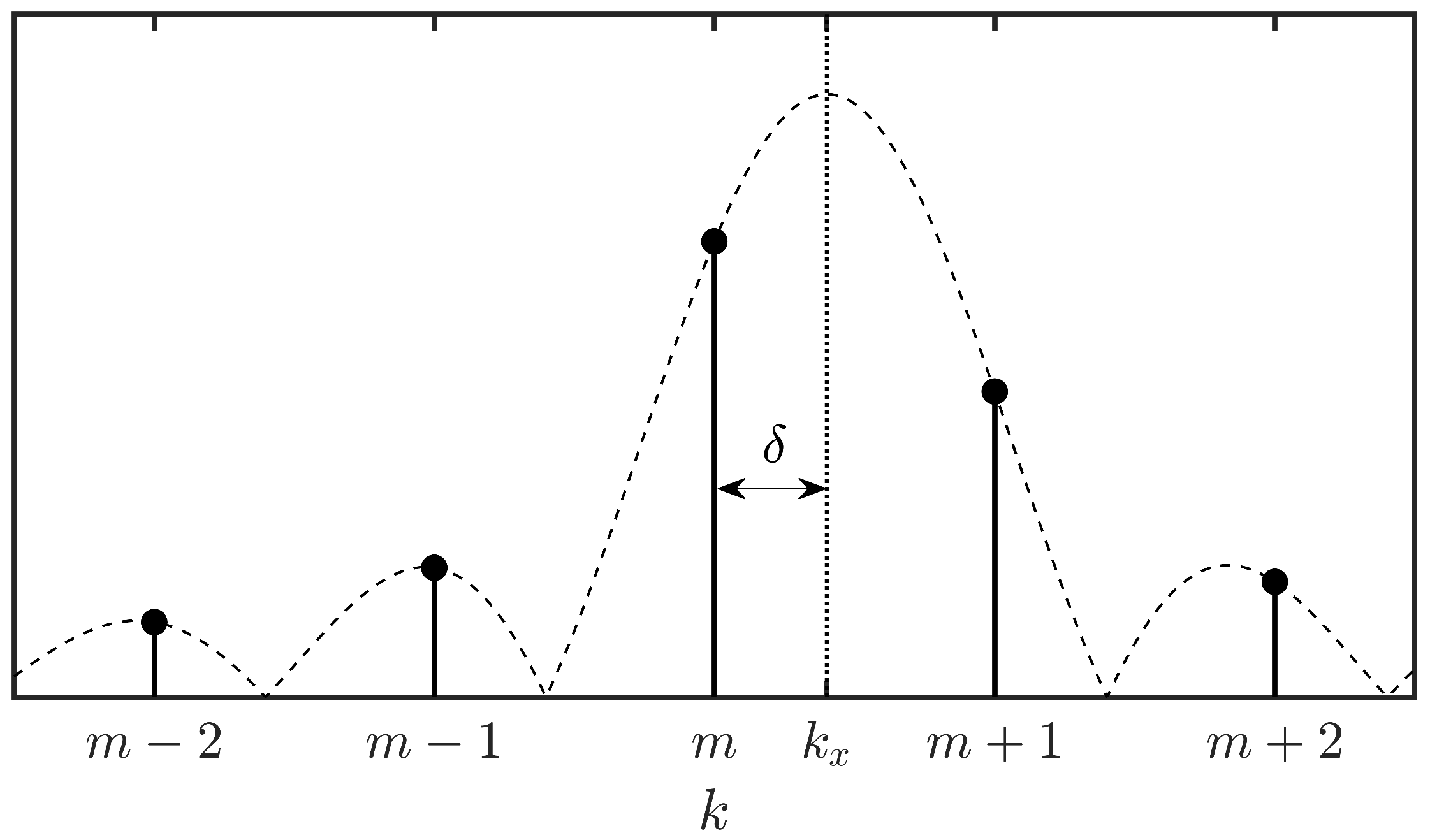
The generic theoretical spectrum of (1), with spectral leakage and when a rectangular window is used, is represented by the dashed black line in Figure 1. The solid vertical lines correspond to the DFT computed frequency components that are spaced at the frequency resolution $\Delta f$.

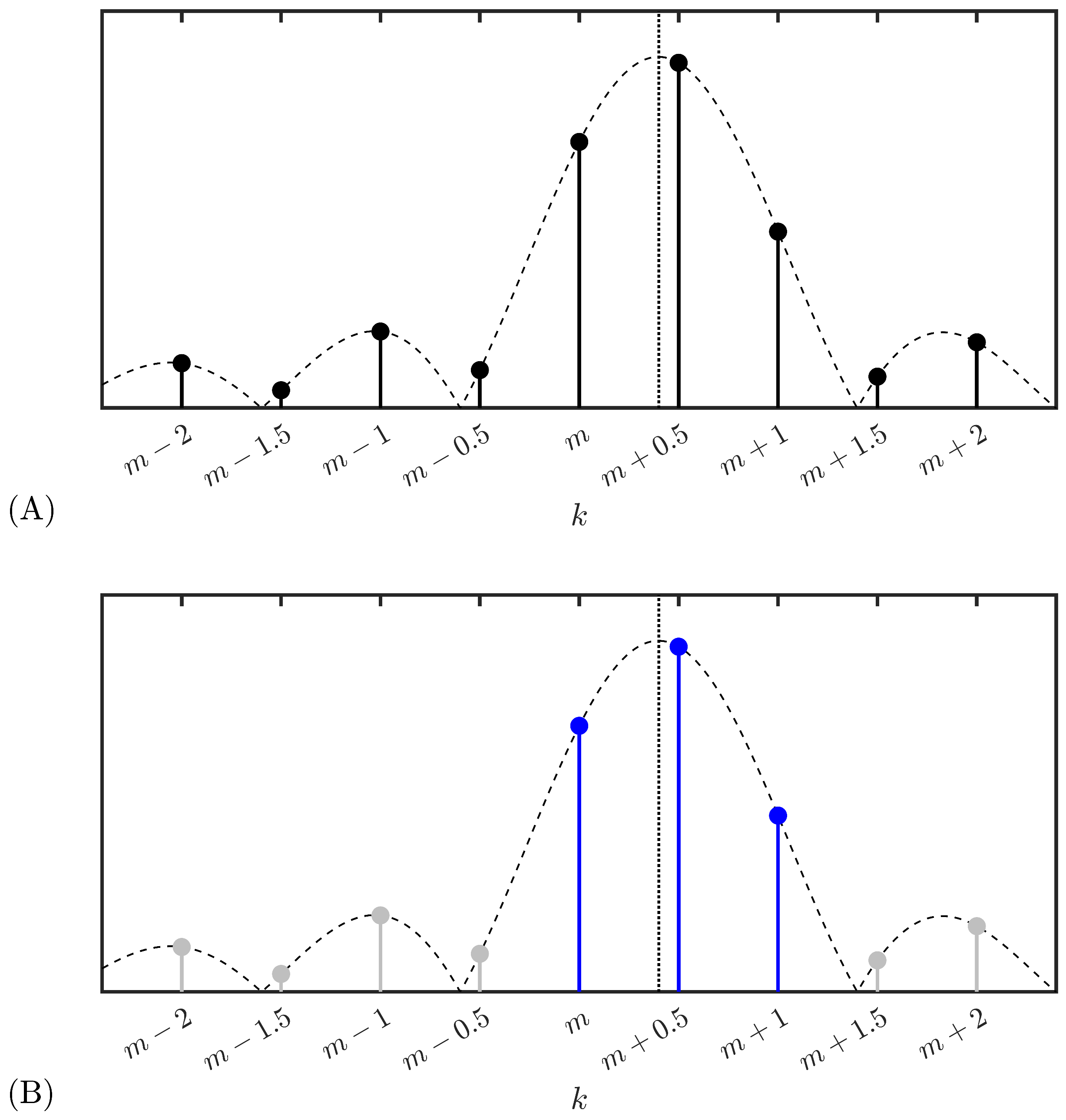
Fan et al. [21] proposed an interpolated DFT method (Fan Alg) that starts by padding the original signal with N zeros to obtain a frequency resolution of $\Delta f/2$ and performing the DFT of the padded signal. Figure 2A shows the theoretical spectrum of the padded signal (dashed line), along with DFT components (vertical black lines) near the signal normalized frequency $k_x$ (vertical dotted line). The algorithm then chooses the component with highest amplitude and its two neighboring components, as shown by the vertical blue lines in Figure 2B, to estimate the sinewave frequency. However, this method requires the computation of an FFT with $2N$ samples.

To increase noise immunity, this work proposes the GFIpDFT algorithm which estimates the frequency, without zero padding, and using extra DTFT components at fractional values of the DFT frequency resolution. The additional fractional DTFT components are spaced by $\alpha =1/p$ (where $p\in \mathbb{N}$). For example, the spectral lines in Figure 2 correspond to a fractional value $\alpha =0.5$.

Without noise and when a rectangular window is considered, the DTFT of (1) is

$$X\left(k\right)={\displaystyle \frac{A}{2}}\left[{\displaystyle \frac{1-e^{-j2\pi (k-k_x)}}{1-e^{-j\frac{2\pi (k-k_x)}{N}}}}{e}^{j\varphi }+{\displaystyle \frac{1-e^{-j2\pi (k+k_x)}}{1-e^{-j\frac{2\pi (k+k_x)}{N}}}}{e}^{-j\varphi }\right].$$

(3)

When the signal frequency is sufficiently away from DC and from $f_s/2$, i.e., $k_x\gg 0$ and $k_x\ll N/2$, Equation (3) can be simplified by neglecting the effect of the second term, which corresponds to the negative frequency spectral image. If in addition a sufficiently large number of samples $N\gg 2\pi |k-k_x|$ is used, (3) can be approximated by

$$X\left(k\right)\approx {\displaystyle \frac{A}{2}}{e}^{j\varphi }{\displaystyle \frac{1-e^{-j2\pi (k-k_x)}}{j\frac{2\pi }{N}(k-k_x)}}.$$

(4)

It should be noted that, for the DFT components, $|k-k_x|\le 0.5$, and therefore, the condition $N\gg 2\pi |k-k_x|$ corresponds to $N>30$. If DTFT with fractional values of k is used, the restriction on the number of samples is further reduced.

The GFIpDFT algorithm begins by performing a Fast Fourier Transform (FFT) on the acquired samples to determine the frequency index m corresponding to its largest spectral component. Since the $m-1$ and $m+1$ components are already available from the FFT, the required $(2/\alpha -2)$ extra DTFT components are computed in the range $(m-1,m+1)$ with step size $\alpha$. To estimate the normalized frequency offset $\delta$, the largest spectral component is considered with index $k=l$, i.e., $X_l=X\left(l\right)$, and the neighboring components $X_{l-\alpha }=X(l-\alpha )$, $X_{l+\alpha }=X(l+\alpha )$, through

$$\widehat{\delta }=\Re \left\{{\displaystyle \frac{\alpha \left[X_{l+\alpha }\left(e^{j2\pi \alpha }-1\right)+X_{l-\alpha }\left(e^{-j2\pi \alpha }-1\right)\right]}{X_{l+\alpha }\left(e^{j2\pi \alpha }-1\right)-X_l\left(e^{j2\pi \alpha }-e^{-j2\pi \alpha }\right)+X_{l-\alpha }\left(e^{-j2\pi \alpha }-1\right)}}\right\}.$$

(5)

The derivation of (5) is presented in Appendix A.

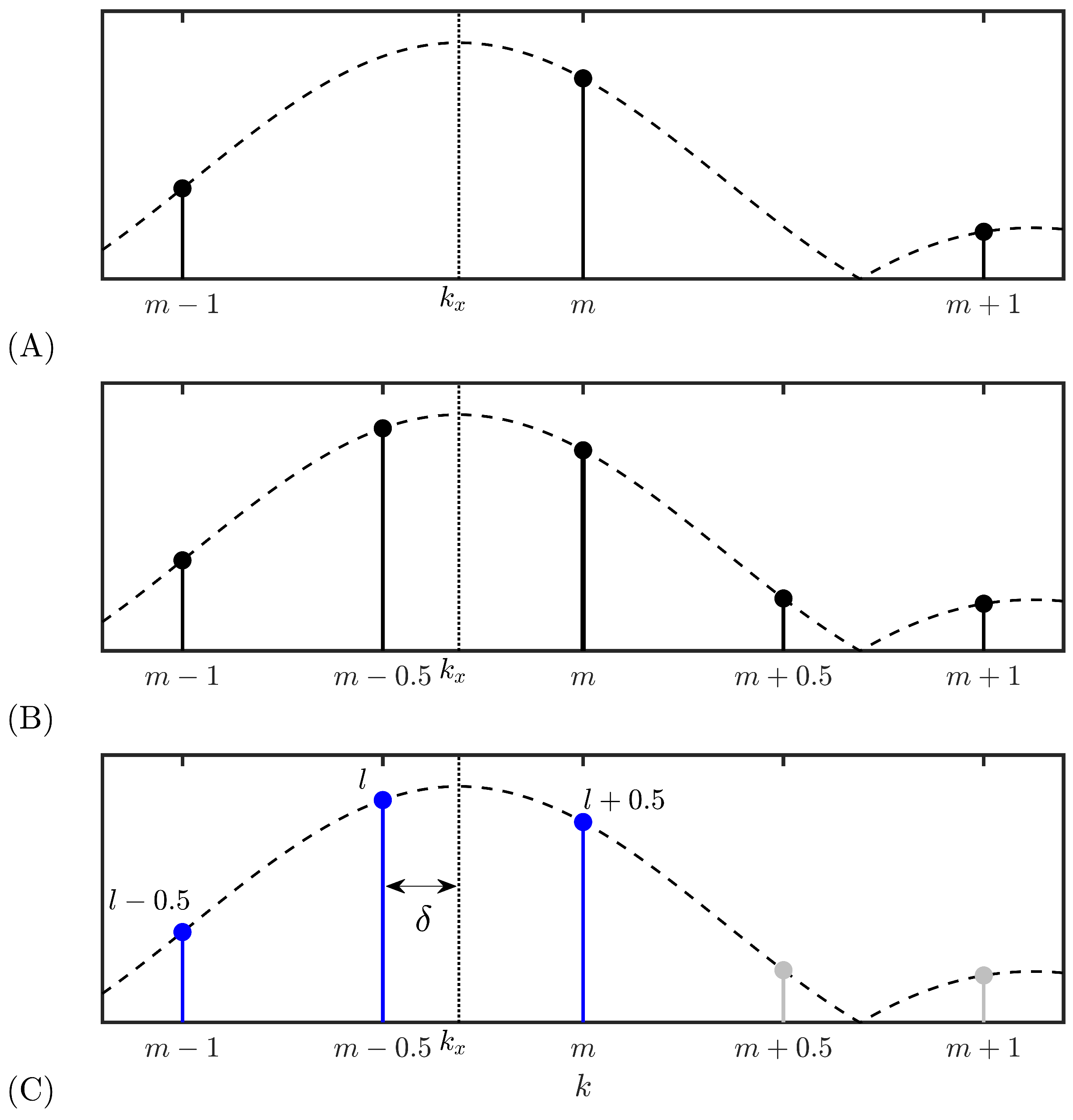
For example, when $\alpha =0.5$ as shown in Figure 3, the algorithm starts with obtaining the DFT of the signal and identifying its largest component m. Figure 3A illustrates this component along with its neighbors at $m-1$ and $m+1$. Two additional DTFT components are computed at the midpoint of the DFT frequencies (i.e., at indices $m-0.5$ and $m+0.5$), as shown in Figure 3B. From these five components, the algorithm uses the component with the highest amplitude and its neighbors, assigning indices l, $l-0.5$ and $l+0.5$, respectively, as shown by the blue lines in Figure 3C. The complex amplitudes of these lines ($X_l$, $X_{l-\alpha }$, and $X_{l+\alpha }$) are used in (5) to estimate the normalized frequency offset $\widehat{\delta }$ and the estimated frequency using (2).

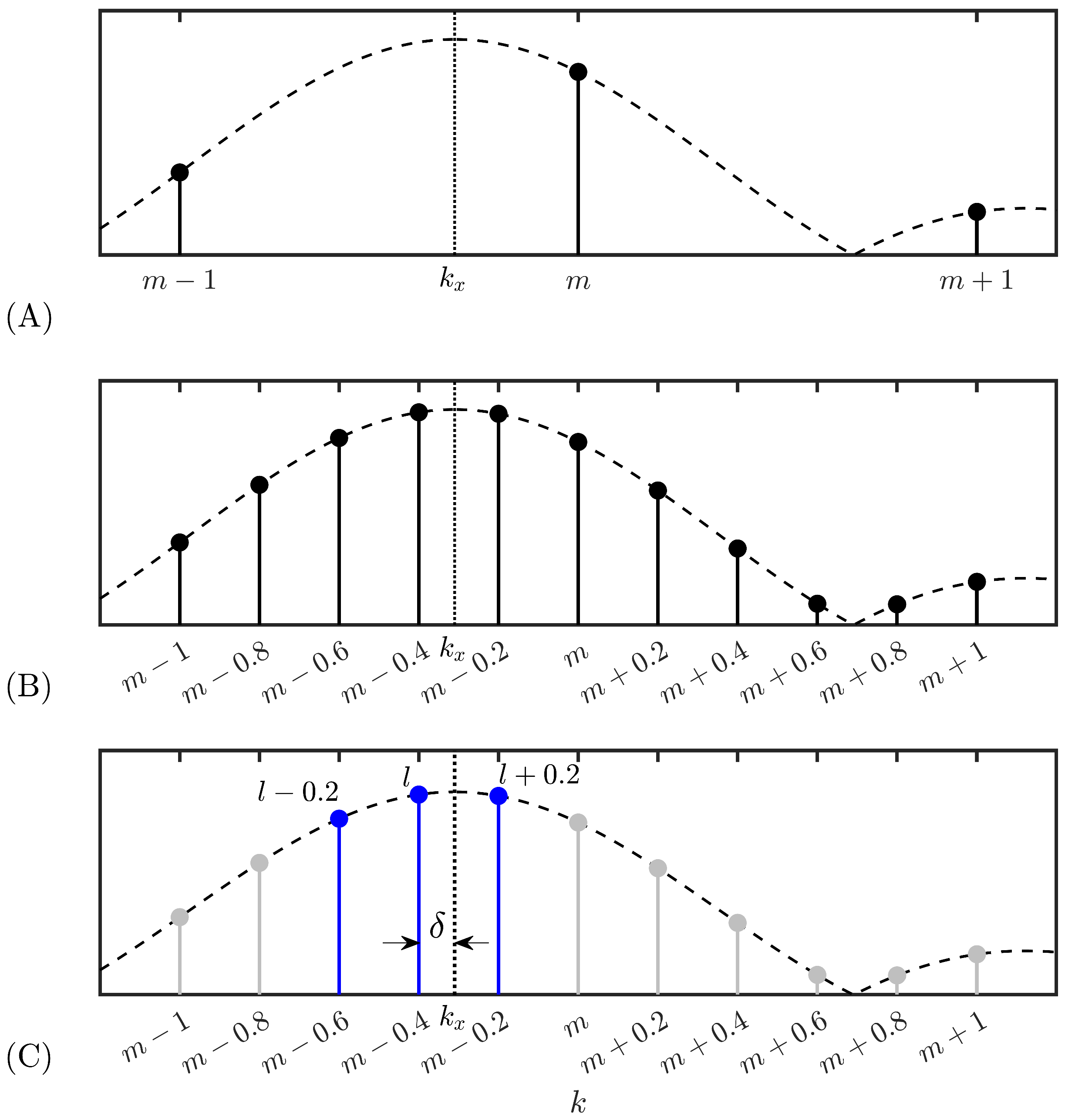
Figure 4 presents a similar example but for the case with $\alpha =0.2$. Initially the signal DFT is obtained and the largest component m and its neighbors are identified as shown in Figure 4A. Then, eight additional DTFT components are computed at locations $m\pm 0.2$, $m\pm 0.4$, $m\pm 0.6$ and $m\pm 0.8$ as shown in Figure 4B. From these eleven components, the algorithm selects the one with the highest amplitude along with its neighboring components, assigning them indices l, $l-0.2$ and $l+0.2$, represented by the blue lines in Figure 4C, which are then used to estimate the signal frequency.

In the GFIpDFT algorithm, the initial DFT is performed with an FFT which has a complexity of $6N{log}_{2}N$ [19], and the additional DTFT components are computed with $(2/\alpha -2)$ non-integer Goertzel filters, each with $3N$ computational complexity [19]. Therefore, the total computational complexity required to calculate the spectral components needed by the GFIpDFT algorithm is $6N\left[({\displaystyle \frac{1}{\alpha }}-1)+{log}_{2}N\right]$. Additionally, a negligible amount of operations is required to apply (5) and (2).

3. Numerical Results

To evaluate the performance of the GFIpDFT algorithm, a simulated sinewave with amplitude $A=\sqrt{2}$ was used, sampled at $f_s$ with N points. Gaussian noise with RMS amplitude ${\sigma }_n$ was added to the signal. Each simulation was repeated ${10}^6$ times, with the signal initial phase $\varphi$, for each repetition, randomly drawn from a uniform distribution over the $[-\pi ,\pi )$ interval. The random phase is used to analyze the performance of the algorithms when there is no trigger used to start the acquisition which results in a random initial phase of the first sample.

The GFIpDFT algorithm, for three different values of $\alpha$ (1, 0.5 and 0.2), is compared with the Fan et al. algorithm (Fan Alg) [21], the FracIpDFT algorithm [19], the IpDFT algorithm [14], the two variants of the algorithm proposed by Aboutanios and Mulgrew (AM Alg1 and AM Alg2) [18] and the square root of the Cramér-Rao Lower Bound [30]

$${\sigma }_{\mathrm{CRLB}}={\displaystyle \frac{f_s}{2\pi }}\sqrt{{\displaystyle \frac{12}{N(N^2-1)\mathrm{SNR}}}}$$

(6)

where $\mathrm{SNR}=A^2/\left(2{\sigma }_n^2\right)$ is the signal-to-noise ratio of the simulated signal.

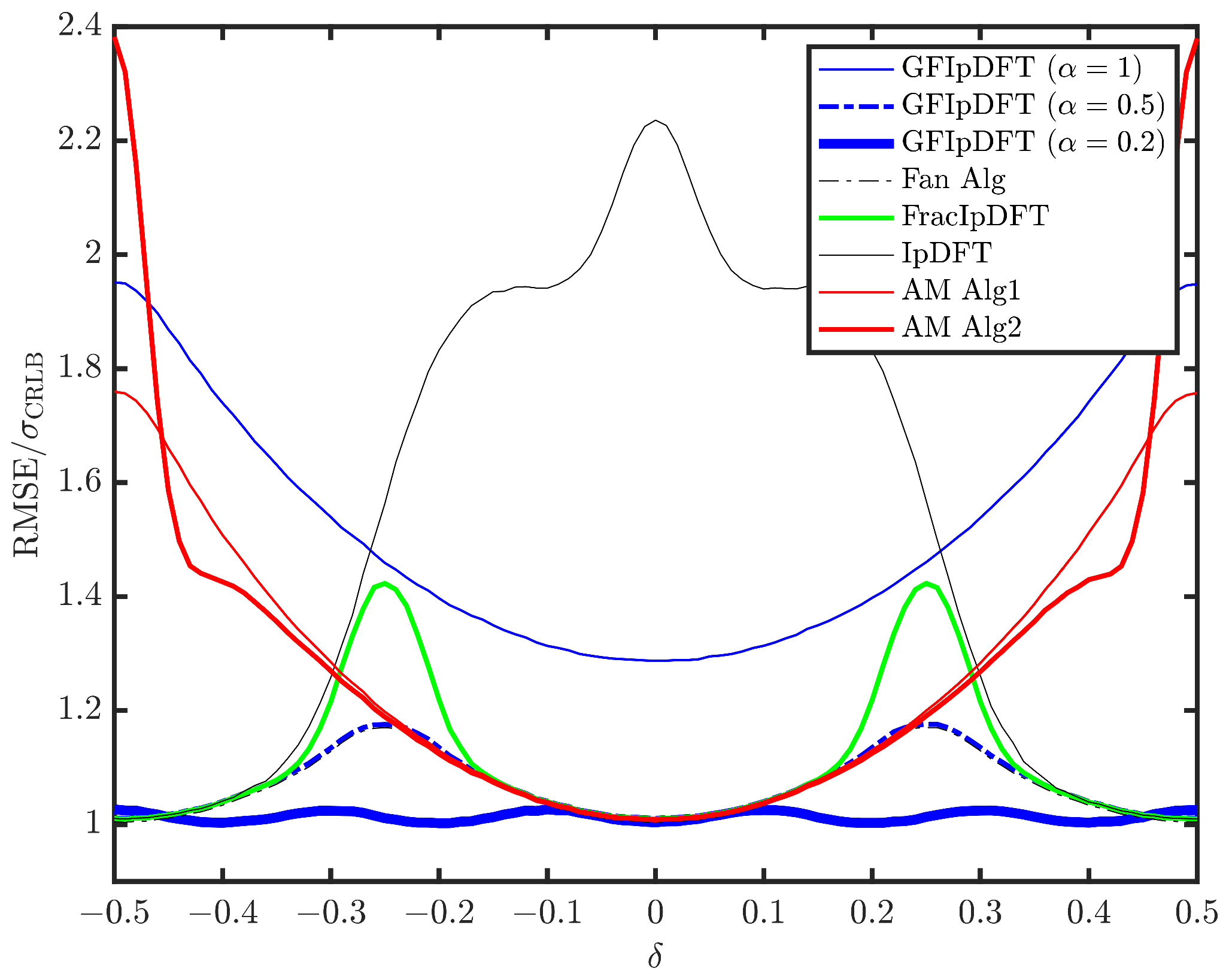
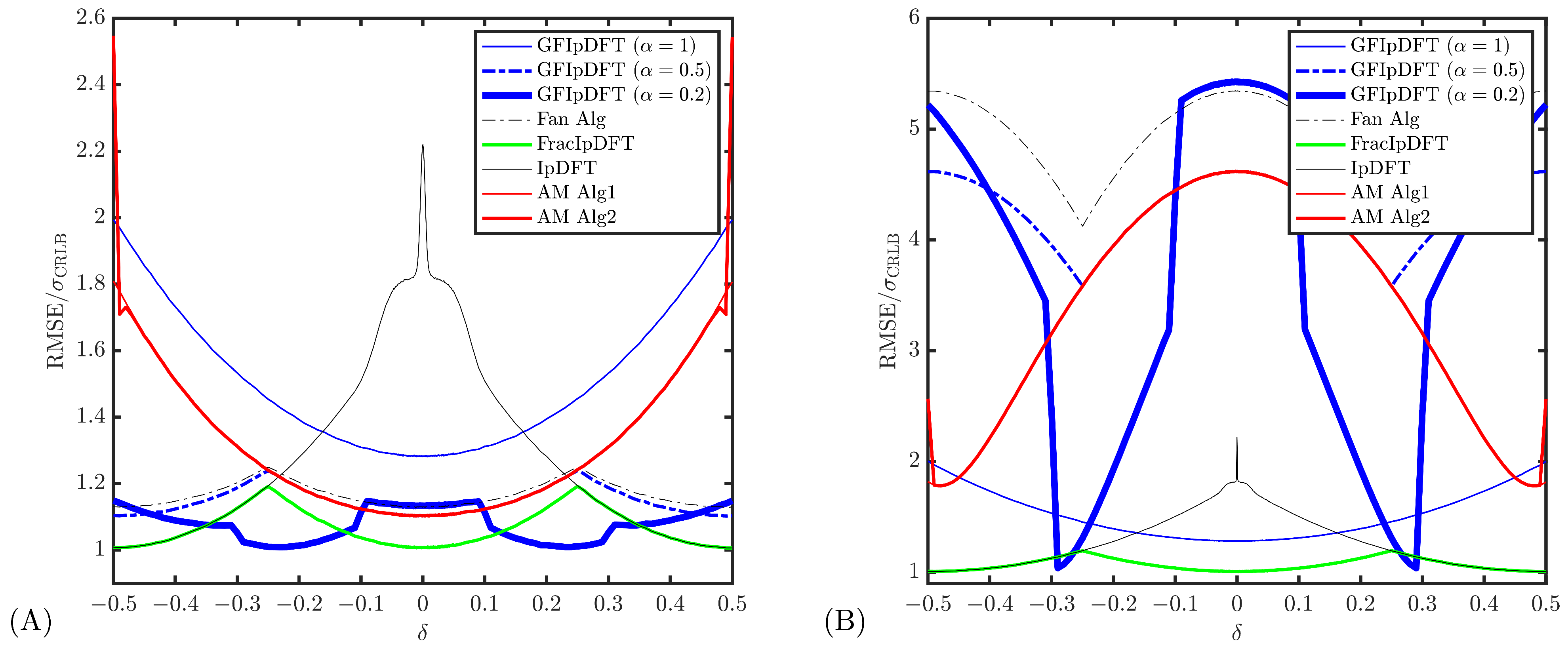
The results presented in Figure 5 and Figure 6 show the RMSE, normalized to ${\sigma }_{\mathrm{CRLB}}$ of the proposed algorithm as a function of the normalized frequency offset $\delta$, and compares the results with other interpolation algorithms. The simulations were performed with $N=500$ samples and $f_s=500$ kHz resulting in a spectral resolution of $\Delta f=1$ kHz. The signal frequency is in the range $\left[123.5,124.5\right]$ kHz which corresponds to $\delta \in \left[-0.5,0.5\right]$.

Figure 5 shows the results for extremely noisy sinewaves with $\mathrm{SNR}=0$ dB, where the GFIpDFT algorithm, with $\alpha =0.2$ (thick blue line), presents the lowest RMSE of the estimated frequency for the full range of frequencies, which remains very close to ${\sigma }_{\mathrm{CRLB}}$. This is due to the three components used in (5) that are closer to each other (when compared to the frequency resolution) and therefore have higher amplitudes, resulting in a higher noise immunity. The GFIpDFT algorithm with $\alpha =0.5$ (dashed blue line), which is similar to the Fan Alg (with the exception of the zero padding used in [21]), is the second-best-performing algorithm, with its performance degrading when the frequency of the signal is located between the DTFT computed components (i.e., near $\delta =\pm 0.25$). The FracIpDFT algorithm has a similar behavior but with worse RMSE. Both AM algorithms exhibit good performance while the signal frequency is close to a DFT bin (i.e., $\delta$ near zero), but worse RMSE as the signal frequency is further away from a DFT bin. The GFIpDFT algorithm with $\alpha =1$ (thin blue line) shows no advantages since it only uses DFT frequency components. The IpDFT algorithm uses only the two highest amplitude DFT components, and in the situation where the signal frequency is near a DFT bin, the second component will have low amplitude, thus being very susceptible to be influenced by the noise in the signal. Therefore, under extremely noisy situations ($\mathrm{SNR}=0$ dB), the IpDFT algorithm is the worst-performing algorithm, except when the signal frequency is near the middle of two DFT components (i.e., $\delta$ near $\pm 0.5$). In these cases, the IpDFT algorithm uses two frequency components with high amplitude, which are less affected by signal noise.

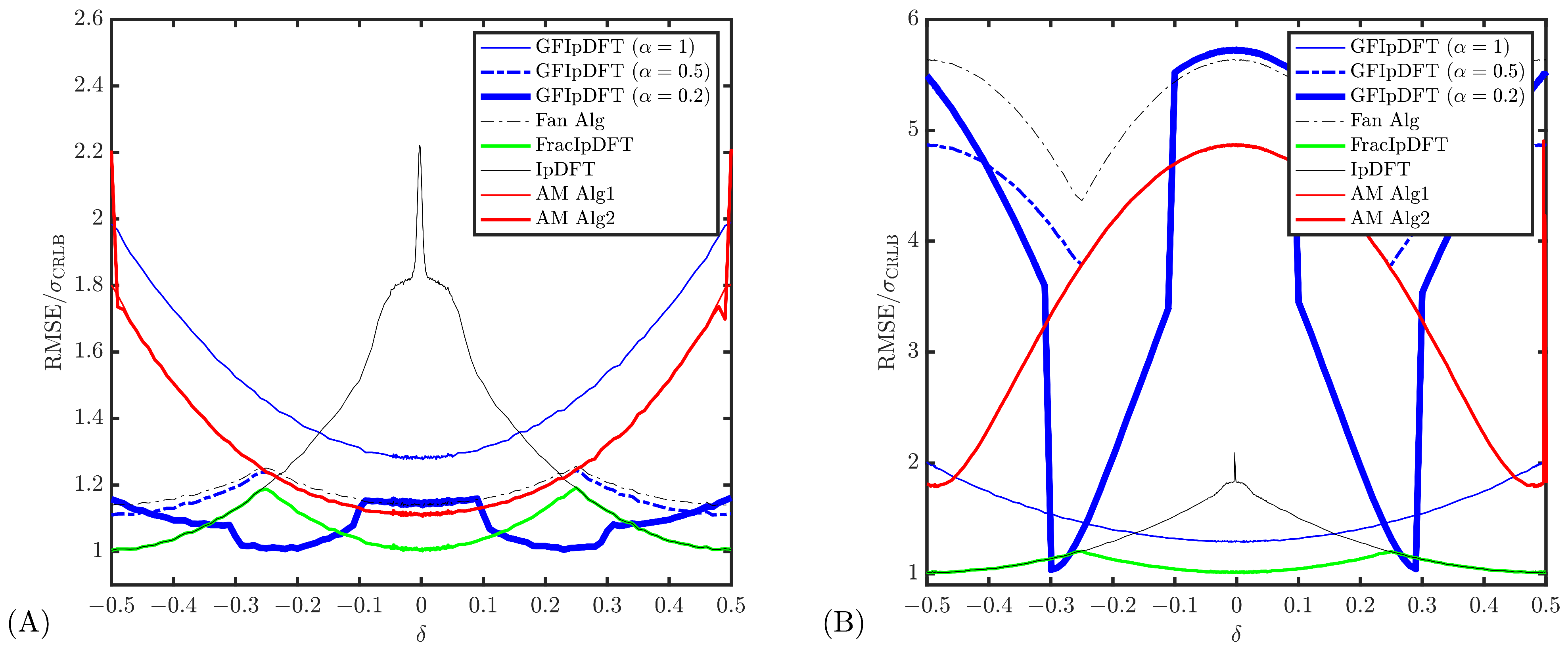
Figure 6 presents the frequency estimation normalized RMSE as a function of the normalized frequency offset ($\delta$) for (A) $\mathrm{SNR}=20$ dB and (B) $\mathrm{SNR}=40$ dB. In the 20 dB case, the GFIpDFT algorithm with $\alpha =0.2$ maintains a low $\mathrm{RMSE}/{\sigma }_{\mathrm{CRLB}}$ ratio and outperforms the other methods except when the signal frequency is close to the DTFT components at multiples of $\Delta f/2$, where the FracIpDFT algorithm provides better results. For small values of $\delta$ (i.e., signal frequencies near DFT bins), the AM algorithms slightly outperform the proposed method, though their performance deteriorates as $\delta$ approaches $\pm 0.5$. A small difference in performance is observed between the Fan Alg results and those of the GFIpDFT algorithm with $\alpha =0.5$ because of the zero padding. The IpDFT algorithm, while effective when the frequency is not near DFT bins, suffers from a pronounced RMSE spike at $\delta =0$ due to the noise-induced random selection of neighboring DFT bins for interpolation.

These effects become more noticeable at lower noise levels, where ${\sigma }_{\mathrm{CRLB}}$ is smaller. In the $\mathrm{SNR}=40$ dB situation, shown in Figure 6B, the FracIpDFT is the best overall performing algorithm, followed closely by the IpDFT algorithm, which continues to show degraded performance at $\delta$ close to 0. At this noise level, most algorithms display high $\mathrm{RMSE}/{\sigma }_{\mathrm{CRLB}}$ values. The results presented indicate that the GFIpDFT algorithm, especially with $\alpha =0.2$, is particularly advantageous for frequency estimation of sinewaves with high noise content.

To further investigate how SNR affects the performance of the proposed GFIpDFT algorithm, Figure 7 and Figure 8 present the normalized estimated frequency RMSE as a function of SNR under different conditions of the number of acquired samples N and normalized frequency offset $\delta$. Figure 7 presents the ratio $\mathrm{RMSE}/f_x$ versus SNR for $N=500$ samples in two scenarios: (A) $\delta =0$, where the signal frequency aligns with a DFT bin, and (B) $\delta =0.25$, where the frequency is between DFT bins. 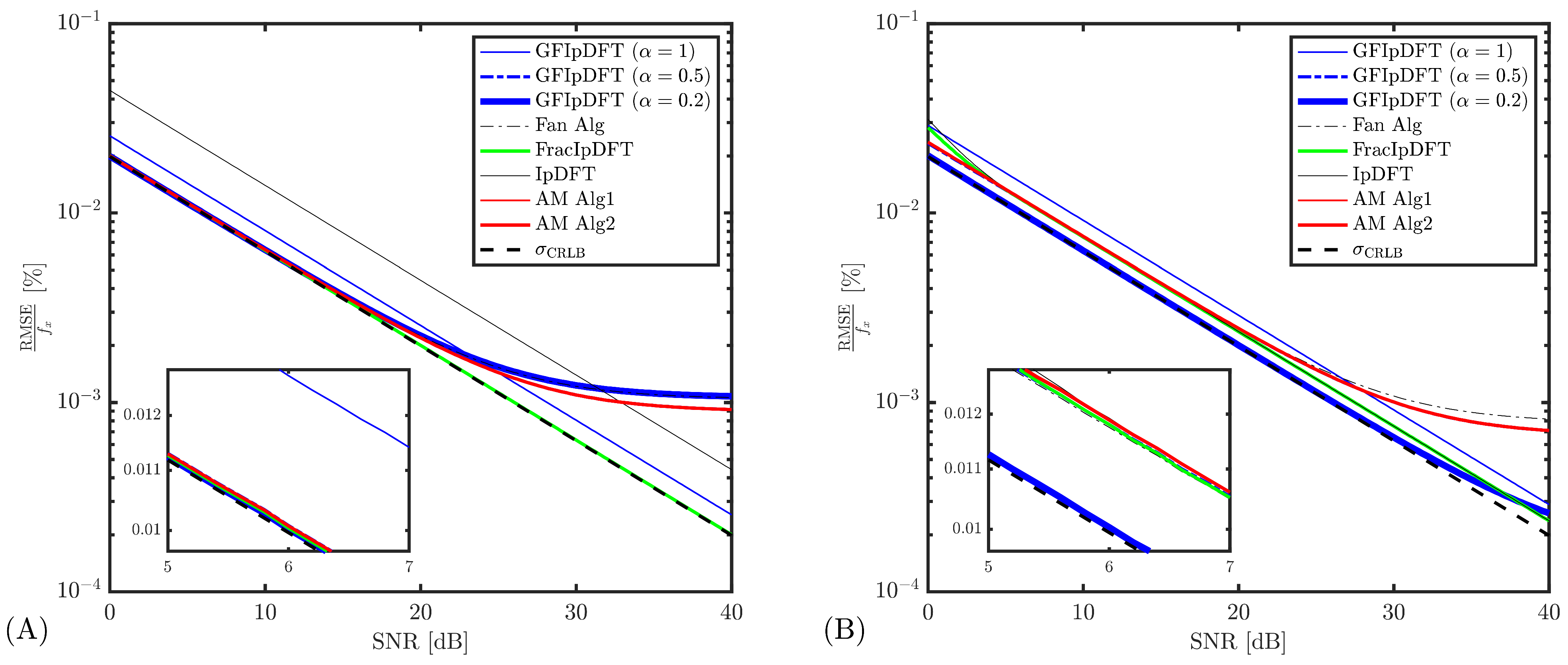In both cases, the GFIpDFT algorithm with $\alpha =0.2$ achieves the lowest RMSE at low SNR levels. However, as SNR improves, the GFIpDFT algorithm and the two AM algorithms exhibit a plateau in the RMSE. This plateau, for GFIpDFT algorithm ($\alpha =0.2$), is more pronounced in (A), occurring at just over 0.001%, while in (B) it appears at higher SNR values and with lower RMSE. The plateaus of the AM and Fan algorithms are similar to that of GFIpDFT algorithm ($\alpha =0.2$) for $\delta =0$, but level off at a higher RMSE for $\delta =0.25$. Although the FracIpDFT and IpDFT algorithms continue to follow the ${\sigma }_{\mathrm{CRLB}}$ trend without leveling off, for $\delta =0.25$, they show greater deviation from the bound at low SNR, while the GFIpDFT algorithm ($\alpha =0.2$) remains close to ${\sigma }_{\mathrm{CRLB}}$ (see inset of Figure 7B).

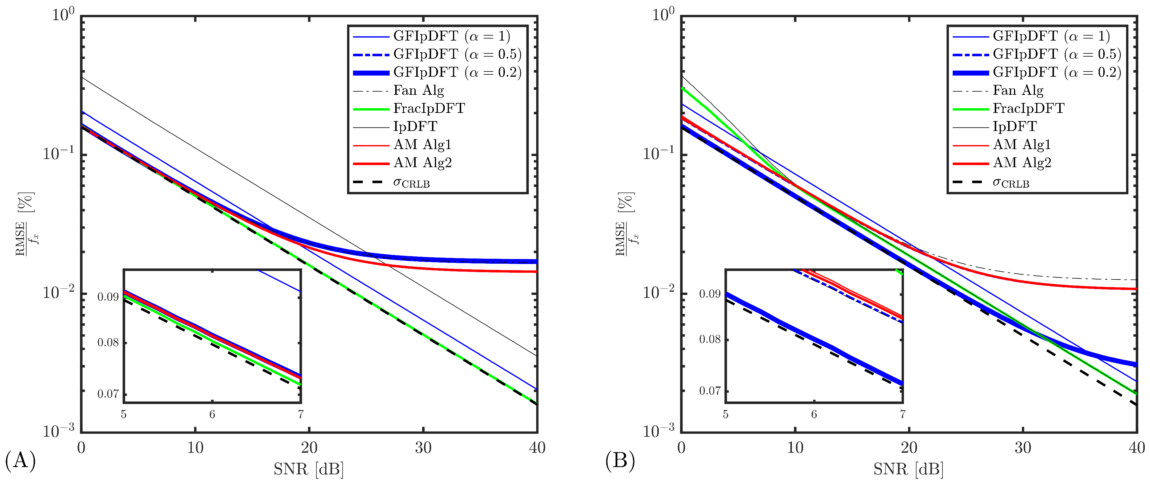
To assess the influence of the number of samples, Figure 8 shows the ratio RMSE$/f_x$ for $N=125$ samples with (A) $\delta =0$ and (B) $\delta =0.25$. The conclusions are similar to those obtained for $N=500$ samples, except that the RMSE values are about one order of magnitude higher. For $\delta =0.25$, the deviation from ${\sigma }_{\mathrm{CRLB}}$ at lower values of SNR for the IpDFT algorithm and FracIpDFT algorithm are more pronounced than what was observed for $N=500$ samples.

The simulation results show that the algorithm that exhibits the best RMSE depends on the number of acquired samples and on the location of the signal frequency in relation to the DTFT computed components. However, for low values of SNR, the GFIpDFT algorithm ($\alpha =0.2$) is consistently the best-performing algorithm, with RMSE values that closely follow the theoretical limit of ${\sigma }_{\mathrm{CRLB}}$.

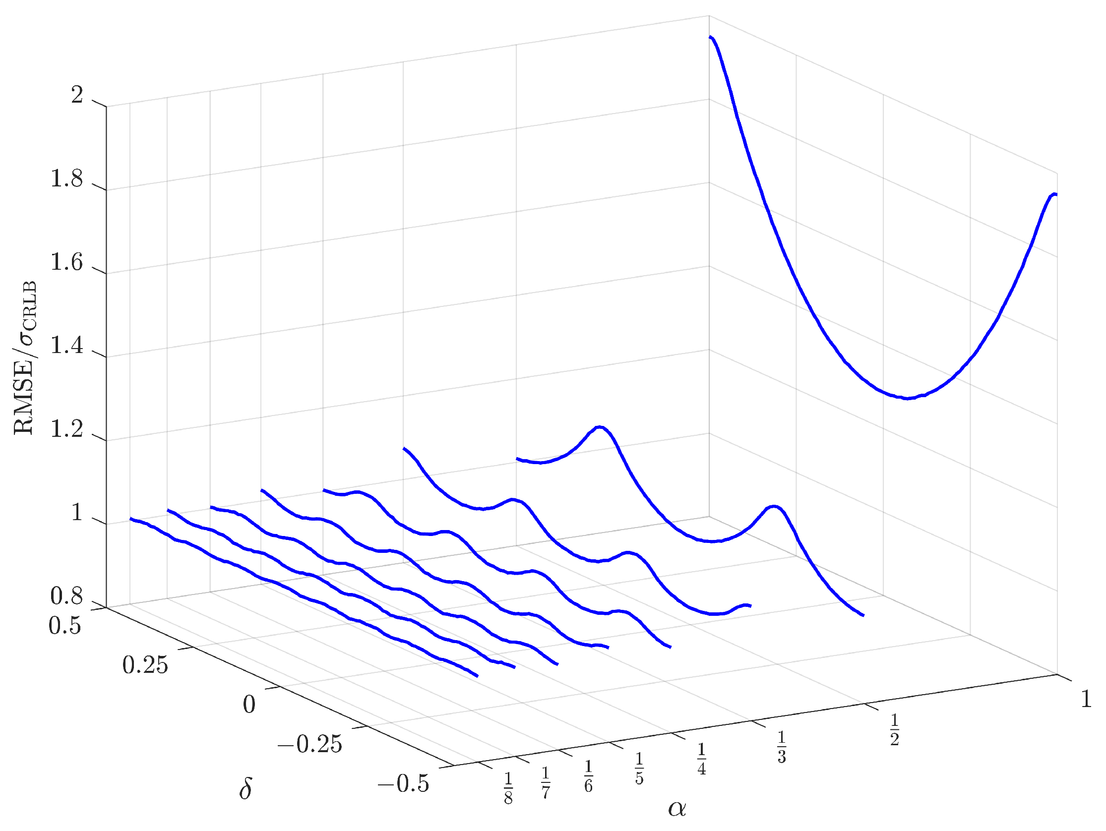
Figure 9 presents an analysis of the behavior of the GFIpDFT algorithm, as the value of the fractional level $\alpha$ is changed, with $\mathrm{SNR}=0$ dB and $N=500$ samples. The RMSE normalized to ${\sigma }_{\mathrm{CRLB}}$ is shown as a function of $\alpha$ and normalized frequency offset $\delta$. There is an improvement in the RMSE value until $\alpha =1/5$, but for lower values of $\alpha$, there are no significant improvements.

4. Measurement Results

To validate the proposed GFIpDFT algorithm, an experimental setup was implemented. An Agilent 33500B waveform generator [31], controlled by IEEE 488.2, was used to generate sinewaves with frequencies in the $\left[123.5,124.5\right]$ kHz range, to replicate the simulation results. This generator can produce random noise with a programmable RMS amplitude and add it to the output sinewave, enabling control of the generated signal SNR. The amplitude of the generated sinewaves was $A=\sqrt{2}$ V and three noise levels were considered with ${\sigma }_n=1$ V, ${\sigma }_n=0.1$ V and ${\sigma }_n=0.01$ V, resulting in $\mathrm{SNR}=0$ dB, $\mathrm{SNR}=20$ dB and $\mathrm{SNR}=40$ dB, respectively. A 16-bit NI USB-6251 data acquisition device [32] was used in the $\pm 10$ V range to acquire ${10}^5$ records, each with $N=500$ samples, at sampling frequency $f_s=500$ kHz.

Ideally, the exact sinewave frequency should be used in the RSME calculations. However, with real measurements, this value is not known due to uncertainty in the generator frequency and uncertainty in the sampling rate. Therefore, for the frequency RMSE calculations, the average frequency obtained using the GFIpDFT algorithm with $\alpha =0.2$ over the ${10}^5$ acquired records for each $\delta$ value was used. This option is confirmed by the estimated RMSE results. An incorrect reference frequency would result in a consistent offset across the RMSE values of the other algorithms, but no such baseline deviation is present which validates the option to select the reference frequency.

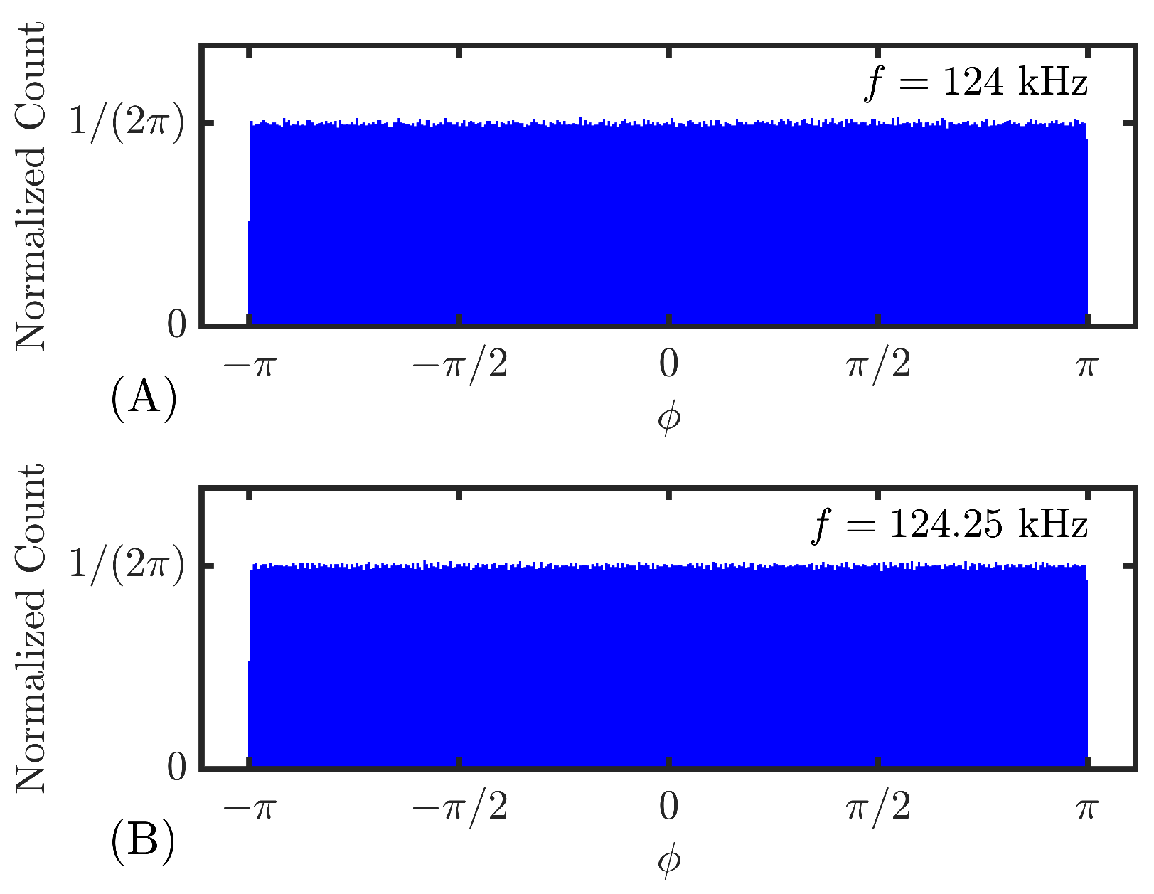
To verify that the condition of the uniformly distributed random initial phase of the generated sinewaves is satisfied, histograms of the phase of each of the ${10}^5$ records were produced. The results are shown in Figure 10A for $f=124$ kHz and $\mathrm{SNR}=40$ dB and in Figure 10B for $f=124.25$ kHz and $\mathrm{SNR}=40$ dB. The phase of each waveform was estimated using the three-parameter sine-fitting algorithm [33], with the above-described reference frequency estimation. The initial phases of the acquired records are uniformly distributed.

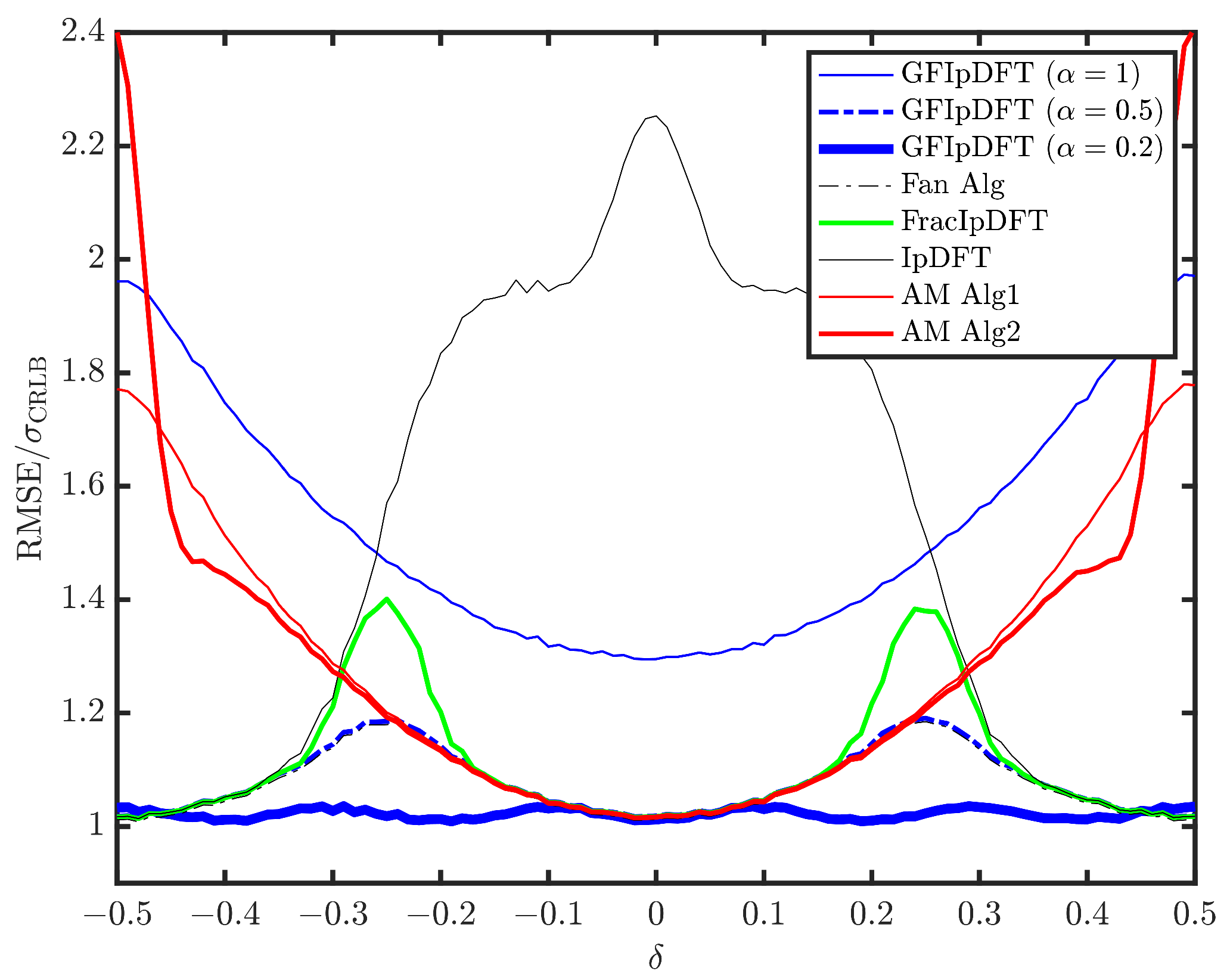
The experimental results for $\mathrm{SNR}=0$ dB, shown in Figure 11, closely replicate the simulation results presented in Figure 5, confirming the behavior of the normalized RMSE of all the algorithms across the $\delta$ range.

In particular, the GFIpDFT algorithm with $\alpha =0.2$ consistently achieved the lowest normalized RMSE, demonstrating its robustness and effectiveness in high-noise conditions. The relative performance of the remaining algorithms follow the pattern observed in the simulations.

Figure 12 presents the experimentally obtained normalized RMSE values for (A) $\mathrm{SNR}=20$ dB and (B) $\mathrm{SNR}=40\mathrm{dB}$. The conclusions drawn from these experimental results are consistent with those obtained from the simulations shown in Figure 6. A slight deviation is observed in the behavior of the AM Algorithm 2 near $\delta \approx \pm 0.5$ in Figure 12B, when compared to the simulation. This discrepancy arises from a small offset in the experimental $f_x/\Delta f$ ratio, which results in a shift in the actual $\delta$ values. This offset is also evident in the RMSE peak of the IpDFT algorithm, which is not exactly at $\delta =0$, as was observed in the simulation results. It should be noted that this shift was expected as it arises from the experimental setup deviations in the signal generation frequency and the data acquisition sampling rate. The shift does not change the validity of the results presented.

The experimental results confirm that, for low values of SNR, the GFIpDFT algorithm with $\alpha =0.2$ is consistently the best-performing algorithm, achieving RMSE values that are close to the theoretical ${\sigma }_{\mathrm{CRLB}}$.

5. Conclusions

This paper introduces the Generalized Fractional Interpolated Discrete Fourier Transform (GFIpDFT) algorithm for frequency estimation of an acquired noisy sinewave and processed with a rectangular window. The algorithm is based on the interpolation of three Discrete Time Fourier Transform (DTFT) components, which can be selected from fractional multiples of the DFT frequency resolution. The algorithm starts by applying the FFT and identifying the largest amplitude FFT bin. For a pre-selected fractional value $\alpha$, additional $\left(2/\alpha -2\right)$ DTFT lines are computed around the peak FFT component using non-integer Goertzel filters. The interpolation is then performed using the component with the highest amplitude and its two neighboring lines. The frequency estimation is based on a closed-form equation, and the complete algorithm is non-iterative. The required number of extra computed DTFT components can be reduced by analyzing the relative amplitude of the already computed components.

The RMSE of the estimated frequency was evaluated across different signal frequencies, SNR levels, and number of acquired samples N. Comparisons with previously published interpolation-based frequency estimation algorithms demonstrated that the proposed method performs particularly well in noisy conditions, closely approaching the Cramér-Rao Lower Bound. However, its performance degrades as the SNR increases, primarily due to the approximations made in deriving the closed-form frequency estimation equation. Therefore, in practice, the use of the GFIpDFT algorithm is advantageous for low SNR, and $\alpha =0.2$ should be used unless there are not sufficient computational resources for its use.

A simple comparison of the time MATLAB, R2025b required to execute each algorithm was performed. To enable the comparison, a reference execution time is used which corresponds to the execution time of the FFT. Accordingly, the results which are presented in

Table 1. Normalized MATLAB execution time of the analyzed algorithms with $N=500$ samples. The normalization is referenced to the FFT execution time with the same number of samples.

Algorithm	Normalized Execution Time
GFIpDFT with $\alpha =1$	11.0
GFIpDFT with $\alpha =0.5$	11.4
GFIpDFT with $\alpha =0.2$	15.3
Fan Alg [21]	25.8
FracIpDFT [19]	15.2
IpDFT [14]	5.4
AM Alg 1 [18]	12.3
AM Alg 2 [18]	11.6

correspond to the ratio between the execution time of the different algorithms and this FFT reference time. This normalization ensures that the results are independent of the used computer processing speed. The IpDFT is the fastest algorithm since it only requires the computation of the FFT followed by the interpolation equations. The AM Alg 1, AM Alg2, FracIpDFT and GFIpDFT algorithms require more execution time due to the number of additional DTFT components that need to be computed. For the GFIpDFT, the number of DTFT components increases for lower fractional values of $\alpha$, i.e., $\alpha =0.5$ requires only two additional components, while $\alpha =0.2$ requires eight additional components. The Fan Alg has the largest execution time because of the initial FFT with $2N$ points. It should be noted that the additional memory required for any $\alpha$ is low when compared with the memory required for the storage of the acquired samples and the initial FFT computation. Therefore, in resource-limited devices, the main constraint will be the time the algorithm requires to provide a frequency estimation, and a guideline of the relative execution time is provided in Table 1.

The simulation results were validated through measurement results, which confirmed the trends observed in the simulations. The proposed GFIpDFT algorithm (with $\alpha =0.2$) maintained its superior performance in low SNR scenarios. The experimental results closely matched the simulated RMSE results, thus validating the proposed GFIpDFT algorithm.

Future work within this topic might include the analysis on the use of other window functions. However, it is not clear if it will be possible to derive a closed-form expression as was demonstrated in Appendix A. In addition, the use of alternative windowing functions which are known to reduce the effect of spectral leakage may introduce other problems such as the requirement to have spectral components closer to the actual frequency sinewave, thus increasing the number of estimated spectral components.